Relic Gravitational Waves from the Chiral Plasma Instability
in the Standard Cosmological Model

Abstract

In the primordial plasma, at temperatures above the scale of electroweak symmetry breaking, the presence of chiral asymmetries is expected to induce the development of helical hypermagnetic fields through the phenomenon of chiral plasma instability. It results in magnetohydrodynamic turbulence due to the high conductivity and low viscosity and sources gravitational waves that survive in the universe today as a stochastic polarized gravitational wave background. In this article, we show that this scenario only relies on Standard Model physics, and therefore the observable signatures, namely the relic magnetic field and gravitational background, are linked to a single parameter controlling the initial chiral asymmetry. We estimate the magnetic field and gravitational wave spectra, and validate these estimates with 3D numerical simulations.

I Introduction

The excess of matter over antimatter on cosmological scales in the universe today is well measured but its origin is not yet established. In studies of early universe cosmology, it is typically assumed that the matter-antimatter asymmetry arose dynamically in the first fractions of a second after the Big Bang through a process called baryogenesis Kolb:1979qa . In addition to creating the baryon asymmetry, e.g., the excess of nuclei over antinuclei, baryogenesis may have created other (possibly unstable) particle asymmetries as well; a few examples include lepton asymmetry Fukugita:1986hr , Higgs asymmetry Servant:2013uwa , neutrino asymmetry Dick:1999je ; Murayama:2002je , and right-chiral electron asymmetry Campbell:1990fa . Some of these are examples of chiral asymmetries, $n_{5}=n_{R}-n_{L}$, namely an excess (or deficit) of right-chiral particles and antiparticles over their left-chiral partners. A particular linear combination of various particle asymmetries, which we call the hypercharge-weighted chiral asymmetry, has attracted interest because of its connections with primordial magnetogenesis Joyce:1997uy through a phenomenon known as the chiral plasma instability Akamatsu:2013pjd .

The primordial magnetic field may survive in the universe today as an intergalactic magnetic field, thereby opening a pathway to test this scenario Neronov:2010gir ; Vachaspati:2020blt . In addition, the primordial magnetic field and its interaction with the turbulent plasma are expected to source gravitational radiation; see Ref. Deryagin:1986qq for pioneering work and Ref. Brandenburg:2021aln for numerical simulations of the gravitational waves induced by the primordial magnetic field originating from the chiral plasma instability. The production of magnetic fields (possibly dark fields) and gravitational wave radiation has also been extensively explored in a different class of theories where the role of the chemical potential is played by axions or axion-like particles Anber:2009ua ; Barnaby:2012xt ; Domcke:2016bkh ; Machado:2018nqk . In our work, we investigate the gravitational wave signatures of a primordial hypercharge-weighted chiral asymmetry via the chiral plasma instability.

Contrary to earlier numerical simulations, we study here a parameter regime that is more realistic in various respects. The resulting gravitational wave energy from our simulations confirm the scaling with the sixth power of the chiral chemical potential and the fifth power of the inverse square root of the chiral dilution parameter, which can be combined into a single parameter, as already found previously Brandenburg:2021aln .

II Description of the model

We consider the primordial Standard Model plasma at temperatures $T\gtrsim 100\ \mathrm{TeV}$ in the phase of unbroken electroweak symmetry. We remain agnostic as to the physics of baryogenesis, but assume that a nonzero hypercharge-weighted chiral asymmetry is present in the plasma initially. We study the growth of an initially vanishingly small hypermagnetic field via the chiral plasma instability and calculate the resulting gravitational wave radiation. The hypermagnetic field generated by the chiral plasma instability is always maximally helical and therefore also leads to the production of maximally circularly polarized gravitational waves. The present work is conceptually different from that of Refs. Brandenburg:2023rul ; Brandenburg:2023aco , where a helical magnetic field was present initially such that the net chirality of the system was balanced to zero by a fermion chirality of opposite sign.

One appealing aspect of our approach is its minimalism: we only assume Standard Model particle physics and the standard cosmological model after reheating. Our only free parameter is the initial hypercharge-weighted chiral asymmetry, which presumably arises from physics beyond the Standard Model. We work in the Lorentz-Heaviside unit system with $\hbar=c=k_{B}=1$. We account for the cosmological expansion using an Friedmann-Lemaître-Robertson-Walker metric with dimensionless scale factor $a(t)$ and set $a_{0}=1$ today. Unless otherwise specified, all dimensionful variables are comoving; this includes conformal time $\mathrm{d}t=\mathrm{d}t_{\mathrm{phys}}/a$, comoving magnetic field ${\bm{B}}=a^{2}{\bm{B}}_{\mathrm{phys}}$, comoving magnetic correlation length $\xi_{\rm M}=\xi_{\mathrm{M,phys}}/a$, comoving temperature $T=aT_{\mathrm{phys}}$, comoving wave number $k=ak_{\mathrm{phys}}$, comoving Hubble parameter $H=aH_{\mathrm{phys}}$ (with $H\equiv(da/dt)/a$), and comoving energy density of any relativistic component (including frozen-in magnetic fields, gravitational waves, etc) $\mathcal{E}=\mathcal{E}_{\mathrm{phys}}a^{4}$. We denote Newton’s gravitational constant by $G$, the Planck mass by $M_{\mathrm{Pl}}=1/\sqrt{G}=1.2\times 10^{19}\,\mathrm{GeV}$, the physical Hubble constant by $H_{\mathrm{phys},0}=100h_{0}\,\mathrm{km}/\mathrm{sec}/\mathrm{Mpc}$, and the critical energy density today by $\mathcal{E}_{\mathrm{cr}}=3H_{0}^{2}/(8\pi G)$. We use the subscript “CPI” to denote the time when the chiral plasma instability (CPI) develops. Assuming that the plasma’s entropy density is conserved between the CPI epoch and today leads to the relation $g_{\ast S,{\text{\sc cpi}}}a_{\text{\sc cpi}}^{3}T_{\mathrm{phys},{\text{\sc cpi}}}^{3}=g_{\ast S,0}a_{0}^{3}T_{\mathrm{phys},0}^{3}$. Taking $g_{\ast S,0}=3.91$ and $T_{\mathrm{phys},0}=0.234\,\mathrm{meV}$ gives

$$\frac{a_{\text{\sc cpi}}}{a_{0}}=(8\times 10^{-19})\bigg{(}\frac{g_{\ast S,{\text{\sc cpi}}}}{106.75}\bigg{)}^{-1/3}\bigg{(}\frac{T_{\mathrm{phys},{\text{\sc cpi}}}}{100\,{\rm TeV}}\bigg{)}^{-1}\;.$$ (1)

We fiducialize the effective number of relativistic degrees of freedom during the CPI epoch to $g_{\ast S,{\text{\sc cpi}}}=106.75$, which is the expected value for Standard Model cosmology at temperatures above $100\,\mathrm{GeV}$. We fiducialize the physical plasma temperature at the CPI epoch to $T_{\mathrm{phys},{\text{\sc cpi}}}=100\,\mathrm{TeV}$.

Chiral magnetic effect.

The chiral plasma instability and chiral magnetic effect (CME) were first studied in the context of a relativistic electron-positron plasma described by quantum electrodynamics (QED). Although chirality is conserved at the classical level for massless electrons, chirality is broken in the quantum theory and this is expressed by the Adler-Bell-Jackiw axial anomaly Bell:1969ts ; Adler:1969gk . A manifestation of the anomalous chiral symmetry is the CME Vilenkin:1980fu : in a QED plasma that possesses a chiral asymmetry, a magnetic field induces a proportional current. The CME corresponds to an anomalous contribution to the electric current density ${\bm{J}}({\bm{x}},t)=\mu_{5}(t){\bm{B}}({\bm{x}},t)$ where $\mu_{5}=2\alpha\tilde{\mu}_{5}/\pi$ is proportional to the chiral chemical potential $\tilde{\mu}_{5}$, $\alpha=e^{2}/4\pi\approx 1/137$ is the electromagnetic fine structure constant, and ${\bm{B}}$ is the magnetic field. Implications of the CME for a turbulent QED plasma have been studied extensively with a combination of analytical techniques and numerical simulations Boyarsky:2011uy ; Boyarsky:2012ex ; Boyarsky:2015faa ; Brandenburg:2017rcb ; Brandenburg:2021aln ; Brandenburg:2023aco ; see also Ref. Kamada:2022nyt for a recent review article.

Adaptation to hypercharge.

The formalism used to study the CME in QED is easily adapted to the hypercharge sector of the Standard Model for a plasma in the phase of unbroken electroweak symmetry at temperatures $T_{\mathrm{phys}}\gtrsim 100\ \mathrm{GeV}$. The quantity of interest is the hypercharge-weighted chiral chemical potential $\tilde{\mu}_{Y,5}(t)$, which is given by $\tilde{\mu}_{Y,5}(t)=\sum_{i}\varepsilon_{i}g_{i}Y_{i}^{2}\tilde{\mu}_{i}(t)$, where the sum runs over all Standard Model particle species (indexed by $i$), $\varepsilon_{i}=\pm 1$ for right/left-chiral particles (and $0$ otherwise), $g_{i}$ is a multiplicity factor (counting color, spin, etc), $Y_{i}$ is the hypercharge of species $i$, and $\tilde{\mu}_{i}$ is the chemical potential that parameterizes the asymmetry (excess of particles over antiparticle partners) in species $i$ via $n_{i}\propto\tilde{\mu}_{i}T^{2}$; see Refs. Kamada:2016eeb ; Kamada:2016cnb for additional details.

Chiral plasma instability.

In the presence of a chiral asymmetry, the equations of magnetohydrodynamics (MHD) are modified due to the CME, and the new equations exhibit a tachyonic instability toward the growth of long-wavelength modes of the magnetic field, which is known as the chiral plasma instability Akamatsu:2013pjd . To illustrate the instability in the hypercharge sector of the primordial plasma, we present the evolution equation for the hyper-magnetic field assuming negligible plasma velocity: $\dot{\bm{B}}_{Y}=\eta_{Y}\nabla^{2}{\bm{B}}_{Y}+(2\alpha_{Y}\tilde{\mu}_{Y,5}/\pi)\eta_{Y}{\bm{\nabla}}\times{\bm{B}}_{Y}$. Here and below, dots represent partial derivatives with respect to conformal time, ${\bm{B}}_{Y}({\bm{x}},t)$ is the hypermagnetic field, $\eta_{Y}=1/\sigma_{Y}$ is the hypermagnetic diffusivity, $\sigma_{Y}$ is the hypercharge conductivity, and $\alpha_{Y}=g^{\prime 2}/4\pi\approx 0.01$ is the hypercharge fine structure constant. Long-wavelength modes of the hypermagnetic field with wave number $k<k_{\text{\sc cpi}}=2\alpha_{Y}|\tilde{\mu}_{Y,5}(t)|/\pi$ experience a tachyonic instability in one of the two circular polarization modes, and their amplitude increases exponentially $\propto\mathrm{exp}(t/t_{\text{\sc cpi}})$. The fastest growing modes have $k=k_{\text{\sc cpi}}/2$, and for these modes $t_{\text{\sc cpi}}=4/\eta_{Y}k_{\text{\sc cpi}}^{2}=\pi^{2}/\eta_{Y}\alpha_{Y}^{2}|\tilde{\mu}_{Y,5}|^{2}$. Assuming a radiation-dominated cosmology with $g_{\ast}=106.75$, the physical plasma temperature at this time is

$$T_{\mathrm{phys},{\text{\sc cpi}}}=\bigl{(}70\ \mathrm{TeV}\bigr{)}\biggl{(}\frac{\eta_{Y}}{0.01T^{-1}}\biggr{)}\biggl{(}\frac{|\tilde{\mu}_{Y,5}|/T}{10^{-3}}\biggr{)}^{2}\;.$$ (2)

In other words, although the chiral asymmetry may be present in the plasma from a very early time, its effect on the hypermagnetic field does not develop until (possibly much) later when the age of the universe is comparable to $t_{\text{\sc cpi}}$ and the plasma has cooled to temperature $T_{\mathrm{phys},{\text{\sc cpi}}}$. Reducing the magnitude of the chiral asymmetry, i.e., assuming a smaller $|\tilde{\mu}_{Y,5}|/T$ initially, delays the onset of the chiral plasma instability.

Chiral asymmetry erasure.

In a relativistic electron-positron plasma described by the theory of QED, the electromagnetic charge is exactly conserved and the chiral charge is approximately conserved. The chiral charge changes in a scattering that converts right-chiral particles into left-chiral particles, or vice versa, and the rate for such ‘spin-flip’ scatterings is proportional the squared electron mass $(m_{e}/T)^{2}$. Although the chiral charge is not exactly conserved, it is important to recognize that it is approximately conserved on time scales that are small compared to the inverse spin-flip rate. Similarly, the hypercharge-weighted chiral asymmetry is eventually driven to zero by scatterings involving the Yukawa couplings; the most relevant processes are Higgs decays and inverse decays with right-chiral electrons. The rate for these chirality-changing reactions is $\Gamma_{\mathrm{f}}\approx 10^{-2}y_{e}^{2}T$, with $y_{e}$ electron Yukawa coupling $y_{e}=\sqrt{2}m_{e}/v\simeq 3\times 10^{-6}$ and assuming a standard radiation-dominated cosmology, these reactions come into equilibrium when the plasma cools to a physical temperature of $T_{\mathrm{phys},\mathrm{f}}\simeq 80\ \mathrm{TeV}$ Bodeker:2019ajh . To ensure that the chiral plasma instability develops before the hypercharge-weighted chiral asymmetry is erased by Higgs decays and inverse decays, it is necessary to have $|\tilde{\mu}_{Y,5}|/T>10^{-3}$. For reference, the observed baryon asymmetry of the universe today corresponds to a much smaller chemical potential of $\tilde{\mu}_{\text{\sf B}}/T\approx 10^{-8}$, but it is not unusual for large chemical potentials to be generated during the course of baryogenesis. New physics such as a matter-dominated phase or an injection of $e_{R}$ asymmetry can change the temperature of chiral asymmetry erasure; for an example, see Ref. Chen:2019wnk .

Magnetogenesis.

As the chiral plasma instability develops, the growing helical hypermagnetic field is accompanied by a depletion of the hypercharge-weighted chiral asymmetry. This is because the hypercharge-weighted chiral number density $n_{Y,5}=\tilde{\mu}_{Y,5}T^{2}/6$ and the hypermagnetic helicity $\mathcal{H}_{B}$ are linked by the chiral anomaly, which imposes $\dot{n}_{Y,5}\propto-\alpha_{Y}\dot{\mathcal{H}}_{\rm M}/\pi$ Joyce:1997uy . If the chiral plasma instability shuts off after the hypercharge-weighted chiral asymmetry depletes by an order one factor, the hypermagnetic helicity can be estimated as $\mathcal{H}_{{\rm M},{\text{\sc cpi}}}\sim\pi|\tilde{\mu}_{Y,5}|T_{\text{\sc cpi}}^{2}/6\alpha_{Y}$. The coherence length and field strength are estimated as $\xi_{{\rm M},{\text{\sc cpi}}}\approx 2\pi/(k_{\text{\sc cpi}}/2)$ and $B_{\text{\sc cpi}}\approx\sqrt{\mathcal{H}_{\rm M}/\xi_{{\rm M},{\text{\sc cpi}}}}$, which gives $\xi_{{\rm M},{\text{\sc cpi}}}\approx(5\times 10^{5}\ \mathrm{cm})(|\tilde{\mu}_{Y,5}|/10^{-3}T)^{-1}$ and $B_{\text{\sc cpi}}\approx(5\times 10^{-11}\ \mathrm{G})\,(|\tilde{\mu}_{Y,5}|/10^{-3}T)$. If the magnetic field evolves according to the inverse cascade scaling (in the fully helical case), $\xi_{\rm M}\propto t^{2/3}$ and $B\propto t^{-1/3}$ Hat84 , until recombination, then the physical coherence length and field strength today (assuming a frozen-in magnetic field and neglecting MHD dynamics at late epochs, after re-ionization) are expected to be on the order of

$$\begin{split}\xi_{\mathrm{M},\mathrm{phys},0}&=\bigl{(}9\times 10^{-4}\ \mathrm{pc}\bigr{)}\biggl{(}\frac{\eta_{Y}}{0.01T^{-1}}\biggr{)}^{2/3}\biggl{(}\frac{|\tilde{\mu}_{Y,5}|/T}{10^{-3}}\biggr{)}^{1/3}\;,\\ B_{\mathrm{phys},0}&=\bigl{(}7\times 10^{-16}\ \mathrm{G}\bigr{)}\biggl{(}\frac{\eta_{Y}}{0.01T^{-1}}\biggr{)}^{-1/3}\biggl{(}\frac{|\tilde{\mu}_{Y,5}|/T}{10^{-3}}\biggr{)}^{1/3}\;.\end{split}$$ (3)

A larger chiral asymmetry leads to a stronger magnetic field on larger length scales today.

Gravitational wave generation.

The time-varying quadrupole moment of the growing hypermagnetic field provides a source of gravitational wave radiation Deryagin:1986qq . As the chiral plasma instability develops, most of the magnetic energy is carried by the modes with coherence length $\xi_{{\rm M},{\text{\sc cpi}}}$ (i.e., the magnetic energy is characterized by a spectrum that peaks at wave number $k_{I}\simeq 2\pi/\xi_{{\rm M},{\text{\sc cpi}}}$). As long as the magnetic field is still growing, however, the induced gravitational wave spectrum peaks at the characteristic wave number $k=2/t_{\text{\sc cpi}}=\eta_{Y}k_{\text{\sc cpi}}^{2}/2$ Brandenburg:2021aln . For $\eta_{Y}k_{\text{\sc cpi}}/2<1$, this wave number is below the cutoff wave number for gravitational waves, $k_{\text{\sc cpi}}$. Above this wave number, very little gravitational wave energy is produced by the chiral plasma instability Brandenburg:2021aln . The gravitational wave cutoff frequency is $f_{\rm GW}\simeq 2k_{I}/(2\pi)\simeq 2/\xi_{{\rm M},{\text{\sc cpi}}}$ (the factor “2” is due to the quadratic nature of the source). Since the gravitational waves’ comoving frequency remains constant, the physical frequency today corresponds to $f_{\mathrm{GW},0}=2/\xi_{{\rm M},{\text{\sc cpi}}}$. Once the CPI stops and $\tilde{\mu}_{Y,5}$ becomes depleted, the low wave number part of the gravitational wave spectrum becomes shallower and the peak moves toward smaller wave numbers.

The energy density carried by the gravitational waves is estimated as $\mathcal{E}_{\mathrm{GW}}\sim(G/2\pi)a_{\text{\sc cpi}}^{-2}\xi_{{\rm M},{\text{\sc cpi}}}^{2}B_{\text{\sc cpi}}^{4}$. This estimate follows from deriving the energy density $\mathcal{E}_{\mathrm{GW}}({\bm{x}},t)$ in the standard way Maggiore:1999vm . Next we define $\Omega_{\mathrm{GW}}=\mathcal{E}_{\mathrm{GW}}/\mathcal{E}_{\mathrm{cr}}$ to be the gravitational wave energy fraction today.

Numerical estimates give

$$\begin{split}f_{\mathrm{GW},0}&=\bigl{(}1\times 10^{5}\ \mathrm{Hz}\bigr{)}\biggl{(}\frac{|\tilde{\mu}_{Y,5}|/T}{10^{-3}}\biggr{)},\\ \Omega_{\mathrm{GW}}h_{0}^{2}&=\bigl{(}7\times 10^{-39}\bigr{)}\biggl{(}\frac{\eta_{Y}}{0.01T^{-1}}\biggr{)}^{2}\biggl{(}\frac{|\tilde{\mu}_{Y,5}|/T}{10^{-3}}\biggr{)}^{6}\;.\end{split}$$ (4)

A larger hypercharge-weighted chiral asymmetry moves the peak of the gravitational wave spectrum to higher frequencies (since the chiral plasma instability develops earlier) and increases the gravitational wave strength. For reference, the LIGO-Virgo-KAGRA gravitational wave interferometer array is sensitive to a stochastic gravitational wave background at the level of $\sim 10^{-7}$ for frequencies of $\sim 10$–$100\ \mathrm{Hz}$ LIGOScientific:2016jlg . The future space-based detectors such as the Laser Interferometer Space Antenna (LISA) will push this sensitivity down to $\sim 10^{-12}$ at frequencies of $\sim 1$–$10\ \mathrm{mHz}$ Bartolo:2018qqn ; Baker:2019nia ; Caprini:2019pxz . At still lower frequencies of $\sim 10^{-9}$–$10^{-7}\ \mathrm{Hz}$, pulsar timing arrays (PTAs), such as Parkes PTA (PPTA) Reardon:2023gzh , European PTA (EPTA) Antoniadis:2023ott , North American Nanohertz Observatory for Gravitational Waves (NANOGrav) NANOGrav:2023hvm , Chinese PTA (CPTA) Xu:2023wog , Indian PTA (InPTA) ChandraJoshi:2022etw , and MeerKAT Pulsar Timing Array (MPTA) Miles:2022lkg are sensitive to a stochastic gravitational wave background at the level of $\Omega_{\mathrm{GW}}h_{0}^{2}\sim 10^{-10}$. Various strategies for probing higher-frequency gravitational waves, even up to the $\mathrm{GHz}$ band, have been explored in recent years; see Ref. Aggarwal:2020olq for a review of these activities. Nevertheless, a detection of gravitational wave radiation at the level expected here, even for $|\tilde{\mu}_{Y,5}|/T\approx 1$, seems far out of reach.

Baryon number overproduction.

The presence of a helical hypermagnetic field in the early universe is expected to give rise to a baryon asymmetry Fujita:2016igl ; Kamada:2016eeb ; Kamada:2016cnb . This is because time-varying hypermagnetic helicity sources baryon and lepton number through the electroweak anomaly Giovannini:1997eg . Specifically, the conversion of a hypermagnetic field into an electromagnetic field at the electroweak epoch at $T_{\mathrm{phys}}\approx 100\ \mathrm{GeV}$ sources baryon number after the electroweak sphaleron has gone out of equilibrium, leading to a boost in the baryon asymmetry Kamada:2016cnb .

The baryon number can easily be over-produced if the magnetic field strength is too large. Avoidance of this baryon-number overproduction imposes an upper bound of $|\tilde{\mu}_{Y,5}|/T\lesssim 10^{-2}$ Domcke:2022uue . This bound is somewhat uncertain as the baryon production calculation depends on a detailed modeling of magnetic field evolution at the Standard Model electroweak crossover Kamada:2016cnb , which is not well understood.

III Numerical simulations

In order to validate the preceding estimates, we have performed three-dimensional numerical simulations using the Pencil Code PC . These simulations allow us to study the growth and evolution of the magnetic field during the chiral plasma instability and to evaluate the spectrum of the resulting gravitational wave radiation.

We model the Standard Model matter and radiation as a single component plasma of charged particles interacting with the hypermagnetic field. Several properties of the plasma are relevant to the evolution: the magnetic diffusivity (for simplicity here and below we suppress the subscript “$Y$”) $\eta(t)=1/\sigma(t)$, the kinematic viscosity $\nu(t)$, the chiral diffusion coefficient $D_{5}(t)$, the chiral depletion parameter $\lambda(t)$, and the chiral chemical potential $\mu_{50}\equiv\mu_{5}(\mathchoice{\mbox{\boldmath$\displaystyle x$}}{\mbox{\boldmath$\textstyle x$}}{\mbox{\boldmath$\scriptstyle x$}}{\mbox{\boldmath$\scriptscriptstyle x$}}{},0)=2\alpha\tilde{\mu}_{5}/\pi$ that enters as an initial condition. One can calculate $\sigma$, $\eta$, $\nu$, and $D_{5}$ from first principles using Standard Model particle physics. The hypercharge conductivity is predicted to be $\sigma\sim T/\alpha\approx 100\,T$ Arnold:2000dr implying $\eta\approx 0.01T^{-1}$, and we assume for simplicity $\eta=\nu=D_{5}$. The chiral depletion parameter $\lambda$ arises from the Standard Model chiral anomalies, and past studies have obtained the prediction $\lambda=192\,\alpha^{2}/T^{2}\simeq 0.02\,T^{-2}$ Rogachevskii:2017uyc ; Brandenburg:2017rcb . The initial chiral chemical potential can be written as $\mu_{50}\approx(6\times 10^{-6}\,T)(\tilde{\mu}_{5}/T/10^{-3})$ by fiducializing to $\tilde{\mu}_{5}/T=10^{-3}$.

Given the limited dynamic range of numerical simulations, it is not possible to set the parameters, $\eta$, $\nu$, $D_{5}$, $\lambda$, and $\mu_{50}$, equal to the Standard Model predictions. Instead we consider sets of simulations with different parameters. They can be distinguished by the relative ordering of the characteristic quantities $v_{\lambda}=\mu_{50}/(\mathcal{E}_{\mathrm{cr}}\lambda)^{1/2}$ and $v_{\mu}=\mu_{50}\eta$. We consider runs in regimes I (where $v_{\lambda}>v_{\mu}$) and II (where $v_{\lambda}<v_{\mu}$).

The simulations solve a coupled system of partial differential equations that account for MHD and the CME Brandenburg:2017rcb to determine the evolution of the magnetic field ${\bm{B}}({\bm{x}},t)$, the energy density of the plasma $\rho({\bm{x}},t)$, the plasma velocity ${\bm{u}}({\bm{x}},t)$, and the chiral chemical potential $\mu_{5}({\bm{x}},t)$. In the following, we solve the following set of equations Rogachevskii:2017uyc

$${\partial\mathchoice{\mbox{\boldmath$\displaystyle A$}}{\mbox{\boldmath$\textstyle A$}}{\mbox{\boldmath$\scriptstyle A$}}{\mbox{\boldmath$\scriptscriptstyle A$}}{}\over\partial t} \!\!=\!\! \mathchoice{\mbox{\boldmath$\displaystyle u$}}{\mbox{\boldmath$\textstyle u$}}{\mbox{\boldmath$\scriptstyle u$}}{\mbox{\boldmath$\scriptscriptstyle u$}}{}\times\mathchoice{\mbox{\boldmath$\displaystyle B$}}{\mbox{\boldmath$\textstyle B$}}{\mbox{\boldmath$\scriptstyle B$}}{\mbox{\boldmath$\scriptscriptstyle B$}}{}+\eta(\mu_{5}\mathchoice{\mbox{\boldmath$\displaystyle B$}}{\mbox{\boldmath$\textstyle B$}}{\mbox{\boldmath$\scriptstyle B$}}{\mbox{\boldmath$\scriptscriptstyle B$}}{}-\mathchoice{\mbox{\boldmath$\displaystyle J$}}{\mbox{\boldmath$\textstyle J$}}{\mbox{\boldmath$\scriptstyle J$}}{\mbox{\boldmath$\scriptscriptstyle J$}}{}),$$ (5)

$${\partial\mu_{5}\over\partial t} \!\!=\!\! -\mathchoice{\mbox{\boldmath$\displaystyle\nabla$}}{\mbox{\boldmath$\textstyle\nabla$}}{\mbox{\boldmath$\scriptstyle\nabla$}}{\mbox{\boldmath$\scriptscriptstyle\nabla$}}{}\cdot(\mu_{5}\mathchoice{\mbox{\boldmath$\displaystyle u$}}{\mbox{\boldmath$\textstyle u$}}{\mbox{\boldmath$\scriptstyle u$}}{\mbox{\boldmath$\scriptscriptstyle u$}}{})-\lambda\eta(\mu_{5}\mathchoice{\mbox{\boldmath$\displaystyle B$}}{\mbox{\boldmath$\textstyle B$}}{\mbox{\boldmath$\scriptstyle B$}}{\mbox{\boldmath$\scriptscriptstyle B$}}{}-\mathchoice{\mbox{\boldmath$\displaystyle J$}}{\mbox{\boldmath$\textstyle J$}}{\mbox{\boldmath$\scriptstyle J$}}{\mbox{\boldmath$\scriptscriptstyle J$}}{})\cdot\mathchoice{\mbox{\boldmath$\displaystyle B$}}{\mbox{\boldmath$\textstyle B$}}{\mbox{\boldmath$\scriptstyle B$}}{\mbox{\boldmath$\scriptscriptstyle B$}}{}+D_{5}\nabla^{2}\mu_{5},\;\;$$ (6)

$${{\rm D}{}\mathchoice{\mbox{\boldmath$\displaystyle u$}}{\mbox{\boldmath$\textstyle u$}}{\mbox{\boldmath$\scriptstyle u$}}{\mbox{\boldmath$\scriptscriptstyle u$}}{}\over{\rm D}{}t} \!\!=\!\! {2\over\rho}\mathchoice{\mbox{\boldmath$\displaystyle\nabla$}}{\mbox{\boldmath$\textstyle\nabla$}}{\mbox{\boldmath$\scriptstyle\nabla$}}{\mbox{\boldmath$\scriptscriptstyle\nabla$}}{}\cdot\left(\rho\nu\bm{\mathsf{S}}\right)-{1\over 4}\mathchoice{\mbox{\boldmath$\displaystyle\nabla$}}{\mbox{\boldmath$\textstyle\nabla$}}{\mbox{\boldmath$\scriptstyle\nabla$}}{\mbox{\boldmath$\scriptscriptstyle\nabla$}}{}\ln\rho+{\mathchoice{\mbox{\boldmath$\displaystyle u$}}{\mbox{\boldmath$\textstyle u$}}{\mbox{\boldmath$\scriptstyle u$}}{\mbox{\boldmath$\scriptscriptstyle u$}}{}\over 3}\left(\mathchoice{\mbox{\boldmath$\displaystyle\nabla$}}{\mbox{\boldmath$\textstyle\nabla$}}{\mbox{\boldmath$\scriptstyle\nabla$}}{\mbox{\boldmath$\scriptscriptstyle\nabla$}}{}\cdot\mathchoice{\mbox{\boldmath$\displaystyle u$}}{\mbox{\boldmath$\textstyle u$}}{\mbox{\boldmath$\scriptstyle u$}}{\mbox{\boldmath$\scriptscriptstyle u$}}{}+\mathchoice{\mbox{\boldmath$\displaystyle u$}}{\mbox{\boldmath$\textstyle u$}}{\mbox{\boldmath$\scriptstyle u$}}{\mbox{\boldmath$\scriptscriptstyle u$}}{}\cdot\mathchoice{\mbox{\boldmath$\displaystyle\nabla$}}{\mbox{\boldmath$\textstyle\nabla$}}{\mbox{\boldmath$\scriptstyle\nabla$}}{\mbox{\boldmath$\scriptscriptstyle\nabla$}}{}\ln\rho\right)$$ (7)

$$-{\mathchoice{\mbox{\boldmath$\displaystyle u$}}{\mbox{\boldmath$\textstyle u$}}{\mbox{\boldmath$\scriptstyle u$}}{\mbox{\boldmath$\scriptscriptstyle u$}}{}\over\rho}\left[\mathchoice{\mbox{\boldmath$\displaystyle u$}}{\mbox{\boldmath$\textstyle u$}}{\mbox{\boldmath$\scriptstyle u$}}{\mbox{\boldmath$\scriptscriptstyle u$}}{}\cdot(\mathchoice{\mbox{\boldmath$\displaystyle J$}}{\mbox{\boldmath$\textstyle J$}}{\mbox{\boldmath$\scriptstyle J$}}{\mbox{\boldmath$\scriptscriptstyle J$}}{}\times\mathchoice{\mbox{\boldmath$\displaystyle B$}}{\mbox{\boldmath$\textstyle B$}}{\mbox{\boldmath$\scriptstyle B$}}{\mbox{\boldmath$\scriptscriptstyle B$}}{})+\eta\mathchoice{\mbox{\boldmath$\displaystyle J$}}{\mbox{\boldmath$\textstyle J$}}{\mbox{\boldmath$\scriptstyle J$}}{\mbox{\boldmath$\scriptscriptstyle J$}}{}^{2}\right]+{3\over 4\rho}\mathchoice{\mbox{\boldmath$\displaystyle J$}}{\mbox{\boldmath$\textstyle J$}}{\mbox{\boldmath$\scriptstyle J$}}{\mbox{\boldmath$\scriptscriptstyle J$}}{}\times\mathchoice{\mbox{\boldmath$\displaystyle B$}}{\mbox{\boldmath$\textstyle B$}}{\mbox{\boldmath$\scriptstyle B$}}{\mbox{\boldmath$\scriptscriptstyle B$}}{},$$

$${\partial\ln\rho\over\partial t} \!\!=\!\! -\frac{4}{3}\left(\mathchoice{\mbox{\boldmath$\displaystyle\nabla$}}{\mbox{\boldmath$\textstyle\nabla$}}{\mbox{\boldmath$\scriptstyle\nabla$}}{\mbox{\boldmath$\scriptscriptstyle\nabla$}}{}\cdot\mathchoice{\mbox{\boldmath$\displaystyle u$}}{\mbox{\boldmath$\textstyle u$}}{\mbox{\boldmath$\scriptstyle u$}}{\mbox{\boldmath$\scriptscriptstyle u$}}{}+\mathchoice{\mbox{\boldmath$\displaystyle u$}}{\mbox{\boldmath$\textstyle u$}}{\mbox{\boldmath$\scriptstyle u$}}{\mbox{\boldmath$\scriptscriptstyle u$}}{}\cdot\mathchoice{\mbox{\boldmath$\displaystyle\nabla$}}{\mbox{\boldmath$\textstyle\nabla$}}{\mbox{\boldmath$\scriptstyle\nabla$}}{\mbox{\boldmath$\scriptscriptstyle\nabla$}}{}\ln\rho\right)$$ (8)

$$+\frac{1}{\rho}\left[\mathchoice{\mbox{\boldmath$\displaystyle u$}}{\mbox{\boldmath$\textstyle u$}}{\mbox{\boldmath$\scriptstyle u$}}{\mbox{\boldmath$\scriptscriptstyle u$}}{}\cdot(\mathchoice{\mbox{\boldmath$\displaystyle J$}}{\mbox{\boldmath$\textstyle J$}}{\mbox{\boldmath$\scriptstyle J$}}{\mbox{\boldmath$\scriptscriptstyle J$}}{}\times\mathchoice{\mbox{\boldmath$\displaystyle B$}}{\mbox{\boldmath$\textstyle B$}}{\mbox{\boldmath$\scriptstyle B$}}{\mbox{\boldmath$\scriptscriptstyle B$}}{})+\eta\mathchoice{\mbox{\boldmath$\displaystyle J$}}{\mbox{\boldmath$\textstyle J$}}{\mbox{\boldmath$\scriptstyle J$}}{\mbox{\boldmath$\scriptscriptstyle J$}}{}^{2}\right],$$

where ${\sf S}_{ij}=(\partial_{j}u_{i}+\partial_{i}u_{j})/2-\delta_{ij}\mathchoice{\mbox{\boldmath$\displaystyle\nabla$}}{\mbox{\boldmath$\textstyle\nabla$}}{\mbox{\boldmath$\scriptstyle\nabla$}}{\mbox{\boldmath$\scriptscriptstyle\nabla$}}{}\cdot\mathchoice{\mbox{\boldmath$\displaystyle u$}}{\mbox{\boldmath$\textstyle u$}}{\mbox{\boldmath$\scriptstyle u$}}{\mbox{\boldmath$\scriptscriptstyle u$}}{}/3$ are the components of the rate-of-strain tensor. We solve Eqs (5)–(8) using the Pencil Code PencilCode:2020eyn , which is a massively parallel MHD code using sixth-order finite differences and a third-order time stepping scheme.

For discussion of the simulation results, we employ “code units.” Times are measured in units of $t_{\ast}=1/H_{\ast}$, lengths in units of $l_{\ast}=c/H_{\ast}$, and energies in units of $E_{\ast}=\mathcal{E}_{\mathrm{cr},\ast}l_{\ast}^{3}$. Setting $\hbar=c=k_{B}=1$ we define $H_{\ast}$ by the relation $H_{\ast}=\sqrt{(8\pi G/3)(\pi^{2}/30)(g_{\ast}T_{\ast}^{4}/a_{\ast}^{2})}$ where $g_{\ast}=100$, $T_{\mathrm{phys},\ast}=T_{\ast}/a_{\ast}=100\,\mathrm{TeV}$, and $T_{\ast}=(g_{\ast S,0}/g_{\ast S,\ast})^{1/3}T_{0}\simeq 8\times 10^{-5}\,\mathrm{eV}$. If the CPI develops at a physical plasma temperature of $100\,\mathrm{TeV}$ then the age of the universe is $\sim 1/H_{\ast}$ and Hubble-scale Fourier modes have $k\sim H_{\ast}$. The linearized gravitational wave equations are solved in wave number space RoperPol:2018sap ,

$$\frac{\partial^{2}}{\partial t^{2}}\tilde{h}_{+/\times}(\mathchoice{\mbox{\boldmath$\displaystyle k$}}{\mbox{\boldmath$\textstyle k$}}{\mbox{\boldmath$\scriptstyle k$}}{\mbox{\boldmath$\scriptscriptstyle k$}}{},t)+k^{2}\tilde{h}_{+/\times}(\mathchoice{\mbox{\boldmath$\displaystyle k$}}{\mbox{\boldmath$\textstyle k$}}{\mbox{\boldmath$\scriptstyle k$}}{\mbox{\boldmath$\scriptscriptstyle k$}}{},t)={6\,H_{\ast}\over t\,\mathcal{E}_{\mathrm{cr}}}\tilde{T}_{+/\times}(\mathchoice{\mbox{\boldmath$\displaystyle k$}}{\mbox{\boldmath$\textstyle k$}}{\mbox{\boldmath$\scriptstyle k$}}{\mbox{\boldmath$\scriptscriptstyle k$}}{},t),$$ (9)

where $\tilde{h}_{+/\times}={\sf e}_{ij}^{+/\times}({\sf P}_{il}{\sf P}_{jm}-{\textstyle{1\over 2}}{\sf P}_{ij}{\sf P}_{lm})\,\tilde{{\sf h}}_{lm}(\mathchoice{\mbox{\boldmath$\displaystyle k$}}{\mbox{\boldmath$\textstyle k$}}{\mbox{\boldmath$\scriptstyle k$}}{\mbox{\boldmath$\scriptscriptstyle k$}}{},t)$ are the Fourier-transformed $+$ and $\times$ modes of $\textstyle h$, with ${\sf e}^{+}_{ij}(\mathchoice{\mbox{\boldmath$\displaystyle k$}}{\mbox{\boldmath$\textstyle k$}}{\mbox{\boldmath$\scriptstyle k$}}{\mbox{\boldmath$\scriptscriptstyle k$}}{})\,\,=\,e_{i}^{1}e_{j}^{1}-e_{i}^{2}e_{j}^{2}$ and ${\sf e}^{\times}_{ij}(\mathchoice{\mbox{\boldmath$\displaystyle k$}}{\mbox{\boldmath$\textstyle k$}}{\mbox{\boldmath$\scriptstyle k$}}{\mbox{\boldmath$\scriptscriptstyle k$}}{})\,=\,e_{i}^{1}e_{j}^{2}+e_{i}^{2}e_{j}^{1}$ being the linear polarization basis, $\mathchoice{\mbox{\boldmath$\displaystyle e$}}{\mbox{\boldmath$\textstyle e$}}{\mbox{\boldmath$\scriptstyle e$}}{\mbox{\boldmath$\scriptscriptstyle e$}}{}^{1}$ and $\mathchoice{\mbox{\boldmath$\displaystyle e$}}{\mbox{\boldmath$\textstyle e$}}{\mbox{\boldmath$\scriptstyle e$}}{\mbox{\boldmath$\scriptscriptstyle e$}}{}^{2}$ are unit vectors perpendicular to $\textstyle k$ and perpendicular to each other, and ${\sf P}_{ij}(\mathchoice{\mbox{\boldmath$\displaystyle k$}}{\mbox{\boldmath$\textstyle k$}}{\mbox{\boldmath$\scriptstyle k$}}{\mbox{\boldmath$\scriptscriptstyle k$}}{})=\delta_{ij}-k_{i}k_{j}$ is the projection operator. $\tilde{T}_{+/\times}$ are defined analogously. We solve Eq. (9) accurate to second order in the time step and use $1024^{3}$ mesh points in all of our calculations. Our initial conditions have a weak seed magnetic field and vanishing plasma velocities, and the chiral chemical potential is homogeneous and equal to the value given above. At each time step, we calculate the spectrum of gravitational wave radiation by solving the gravitational wave equation sourced by the stress-energy of the plasma and magnetic field; see Ref. RoperPol:2018sap for details regarding our computational approach.

Table 1: Summary of Runs discussed in this paper. Runs B1, B10, A1, and A12 of Ref. Brandenburg:2021aln are included for comparison. In the last row, theoretically expected values are listed where $\eta_{2}=\eta_{Y}/(0.01T^{-1})$ and $\mu_{3}=\tilde{\mu}_{Y,5}/10^{-3}T$.

Run $\eta H_{\ast}$ $(\mathcal{E}_{\mathrm{cr}}\lambda)^{1/2}/H_{\ast}$ $\mu_{50}/H_{\ast}$ $v_{\mu}$ $v_{\lambda}$ $\eta\mu_{50}^{2}/H_{\ast}$ $k_{1}/H_{\ast}$ ${\cal E}_{\rm M}^{\max}/{\mathcal{E}}_{\rm cr}$ ${\cal E}_{\rm GW}^{\rm sat}/{\mathcal{E}}_{\rm cr}$ $q$ B1 $1\times 10^{-6}$ $2\times 10^{4}$ $10^{4}$ $1\times 10^{-2}$ $5\times 10^{-1}$ $1\times 10^{2}$ $1\times 10^{2}$ $1.6\times 10^{-2}$ $4.7\times 10^{-12}$ $0.027$ B10 $1\times 10^{-3}$ $2\times 10^{4}$ $10^{4}$ $1\times 10^{1}$ $5\times 10^{-1}$ $1\times 10^{5}$ $1\times 10^{2}$ $6.0\times 10^{-2}$ $6.0\times 10^{-9}$ $12$ A1 $1\times 10^{-6}$ $5\times 10^{4}$ $10^{4}$ $1\times 10^{-2}$ $2\times 10^{-1}$ $1\times 10^{2}$ $1\times 10^{2}$ $4.6\times 10^{-3}$ $8.9\times 10^{-14}$ $0.032$ A12 $5\times 10^{-3}$ $5\times 10^{4}$ $10^{4}$ $5\times 10^{1}$ $2\times 10^{-1}$ $5\times 10^{5}$ $5\times 10^{1}$ $9.2\times 10^{-3}$ $3.0\times 10^{-10}$ $18$ X1 $5\times 10^{-8}$ $10^{10}$ $10^{6}$ $5\times 10^{-2}$ $1\times 10^{-4}$ $5\times 10^{4}$ $5\times 10^{3}$ $2.4\times 10^{-9}$ $8.8\times 10^{-31}$ $0.39$ X2 $5\times 10^{-9}$ $10^{10}$ $10^{6}$ $5\times 10^{-3}$ $1\times 10^{-4}$ $5\times 10^{3}$ $5\times 10^{3}$ $2.4\times 10^{-9}$ $1.6\times 10^{-30}$ $0.53$ X3 $5\times 10^{-10}$ $10^{10}$ $10^{6}$ $5\times 10^{-4}$ $1\times 10^{-4}$ $5\times 10^{2}$ $5\times 10^{3}$ $2.4\times 10^{-9}$ $1.1\times 10^{-30}$ $0.44$ X4 $5\times 10^{-11}$ $10^{10}$ $10^{6}$ $5\times 10^{-5}$ $1\times 10^{-4}$ $5\times 10^{1}$ $5\times 10^{3}$ $2.3\times 10^{-9}$ $3.1\times 10^{-31}$ $0.12$ Y1 $5\times 10^{-8}$ $7\times 10^{11}$ $10^{6}$ $5\times 10^{-2}$ $1\times 10^{-6}$ $5\times 10^{4}$ $5\times 10^{3}$ $4.9\times 10^{-13}$ $3.6\times 10^{-38}$ $0.39$ Y2 $5\times 10^{-8}$ $7\times 10^{11}$ $10^{6}$ $5\times 10^{-2}$ $1\times 10^{-6}$ $5\times 10^{4}$ $2\times 10^{3}$ $4.4\times 10^{-13}$ $3.2\times 10^{-37}$ $1.3$ Y3 $5\times 10^{-8}$ $7\times 10^{11}$ $10^{6}$ $5\times 10^{-2}$ $1\times 10^{-6}$ $5\times 10^{4}$ $1\times 10^{3}$ $3.3\times 10^{-13}$ $6.9\times 10^{-37}$ $2.5$ exp $10^{-15}\eta_{2}$ $6\times 10^{12}$ $5\times 10^{7}\mu_{3}$ $6\times 10^{-8}\eta_{2}\mu_{3}$ $8\times 10^{-6}\mu_{3}$ $3\eta_{2}\mu_{3}^{2}$ — $6\times 10^{-15}\mu_{3}^{2}$ $7\times 10^{-39}\eta_{2}^{2}\mu_{3}^{6}$ —

In Table LABEL:Tsummary, we summarize the parameters used in our simulations, including the smallest wavenumber $k_{1}$, and the key results. We consider two series of runs that we refer to as X and Y. We also compare with two pairs of runs, A1 and A12, as well as B1 and B10, both from Ref. Brandenburg:2021aln . where $\mu/v_{\lambda}$ increases from 0.02 and 0.05 to 20 and 250, respectively. Also the efficiency parameters increases from 0.03 to 12 and 18, respectively. The runs of series X and Y are subdivided further into Runs X1–X4 and Runs Y1–Y3. Our runs of series X have increasing values of $v_{\mu}$ and cross from regime II (for Run X1) into regime I (for Run X4). For the runs of series X, we take $\eta=\nu=D_{5}=5\times 10^{-11}/H_{\ast}$, $\mathcal{E}_{\mathrm{cr}}\lambda=10^{20}\,H_{\ast}^{2}$, and $\mu_{50}=10^{6}\,H_{\ast}$. We also give the efficiency of gravitational wave production,

$$q=(k_{\rm peak}/H_{\ast})\left.\sqrt{{\cal E}_{\rm GW}^{\rm sat}{\mathcal{E}}_{\rm cr}}\right/{\cal E}_{\rm M}^{\max},$$ (10)

where we estimate $k_{\rm peak}=k_{\mu}\min(1,v_{\mu}/v_{\lambda})$ where $k_{\mu}=\mu_{50}/2$. This means that $k_{\rm peak}=k_{\mu}$ when $v_{\mu}>v_{\lambda}$ (regime II) and $k_{\rm peak}=k_{\lambda}/4$ when $v_{\mu}<v_{\lambda}$ (regime I); see Ref. Brandenburg:2017rcb .

In the last row of Table LABEL:Tsummary, we compare with the theoretically expected values. Obviously, our values of $\eta$ are about seven orders of magnitude too large. This reflects the fact that our simulations are unable to capture a sufficiently large range of length scales. Consequently, also our values of $v_{\mu}$ are by about six orders of magnitude too large. Furthermore, $\eta\mu_{50}^{2}/H_{\ast}$ is by about four orders of magnitude too large. Most of the other simulation values in the table are not so far from the theoretically expected values.

The evolution of the magnetic and gravitational wave energy spectra for Run X4 is shown in Fig. 1. The energy densities may be written as $\mathcal{E}=\int_{0}^{\infty}\!\mathrm{d}k\,E(k)$ where $k$ is the wave number and $E(k)$ is the energy spectrum. For the parameters of Run X4, the instability length scale corresponds to a wavenumber of $k_{\text{\sc cpi}}=10^{6}H_{\ast}$, which agrees with the wave number above which $E_{\rm GW}(k)$ drops sharply. The instability time scale normalized to the Hubble time is $t_{\text{\sc cpi}}H_{\ast}=0.08$, which is about 100 times longer than the time step. The magnetic energy spectrum grows initially for modes with $k\approx k_{\text{\sc cpi}}/2=5\times 10^{5}H_{\ast}$ (see the upper set of dotted lines in Fig. 1). Later, the peak evolves to smaller $k$ with an inverse cascade scaling, which is consistent with earlier simulations Brandenburg:2017rcb . The generated magnetic field is then maximally helical; see Fig. 8(b) of Ref. Brandenburg:2021bfx .

The gravitational wave energy spectra grow in time as long as the magnetic energy has not yet reached its maximum. In this phase, as discussed above, the gravitational wave spectrum is expected to peak at the characteristic wave number $k=2/t_{\text{\sc cpi}}=\eta k_{\text{\sc cpi}}^{2}/2=25\,H_{\ast}$, which is here much smaller than $k_{\text{\sc cpi}}=10^{6}H_{\ast}$, but larger than the horizon wave number, $k=H_{\ast}$. When the magnetic energy density has reached its maximum value, the gravitational wave spectrum has nearly saturated and is then approximately independent of $k$ for $k<k_{\text{\sc cpi}}/2$. In principle, it is possible to have a declining $k^{-2}$ spectrum in the range $\eta k_{\text{\sc cpi}}^{2}/2\leq k\leq k_{\text{\sc cpi}}$, but this is only seen in our models with larger diffusivity. The absence of a $k^{-2}$ subrange in the gravitational wave spectrum could also be an artifact of insufficient numerical resolution. In any case, once the gravitational wave spectrum saturates, we would expect the development of a flat ($E_{\rm GW}\propto k^{0}$) spectrum. Such a flat spectrum is expected to extend all the way to the horizon wave number $k=H_{\text{\sc cpi}}$ RoperPol:2019wvy ; RoperPol:2022iel ; Sharma:2022ysf . Therefore, the total gravitational wave energy is expected to be proportional to $k_{\text{\sc cpi}}/2-H_{\ast}$. However, since $k_{\text{\sc cpi}}/2$ is already much larger than our lower cutoff value $k_{1}$, the error in our estimate of ${\cal E}_{\rm GW}\propto k_{\text{\sc cpi}}/2-k_{1}$ is negligible.

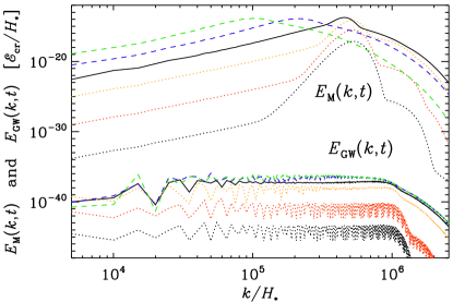
Figure 1: Spectra (per linear wave number interval) of magnetic energy $E_{\rm M}(k,t)$ (upper curves) and gravitational wave energy $E_{\rm GW}(k,t)$ (lower curves) from the chiral plasma instability and turbulent MHD evolution for Run X4, where $\mu_{5}=10^{6}\,H_{\ast}$, $\mathcal{E}_{\mathrm{cr}}\lambda=10^{20}/H_{\ast}$, $\eta=5\times 10^{-11}\,H_{\ast}$ which implies $v_{\lambda}=10^{-4}$ and $v_{\mu}=5\times 10^{-5}$ (corresponding to regime I). The solid curves are for $tH_{\ast}=2.98$, when ${\cal E}_{\rm M}$ is maximum. The dotted curves are for $tH_{\ast}=2.41$ (black), $2.56$ (red), and $2.71$ (orange), before ${\cal E}_{\rm M}$ is maximum, while the dashed curves are for $tH_{\ast}=3.66$ (blue) and $tH_{\ast}=5.37$ (green), when ${\cal E}_{\rm M}$ is decaying.

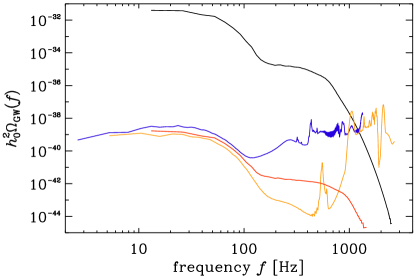
Figure 2: Comparison of $h_{0}^{2}\Omega_{\rm GW}(f)$ versus $f$ for runs with $k_{1}/H_{\ast}=10^{3}$ (Run Y3, blue), $2\times 10^{3}$ (Run Y2, orange), and $5\times 10^{3}$ (Run Y1, red), with $\lambda=49\times 10^{22}H_{\ast}^{2}/\mathcal{E}_{\mathrm{cr},\ast}$ and $\eta=5\times 10^{-8}H_{\ast}^{-1}$ with $H_{0}=100\,h_{0}\,{\rm km}\,{\rm s}^{-1}\,{\rm Mpc}^{-1}$. Run X4 with with $\lambda=10^{20}H_{\ast}^{2}/\mathcal{E}_{\mathrm{cr},\ast}$ and again $\eta=5\times 10^{-8}H_{\ast}^{-1}$ is shown as the black line for reference.

In Fig. 2, we show gravitational wave spectra for a few runs with smaller values of the minimum wave number in the simulations. We see that the spectra remain nearly flat, but the spectra are also becoming more irregular at large wave numbers. This is likely an artifact of insufficient numerical resolution. We also see that most of the gravitational wave energy is at frequencies below about $1\,\,{\rm kHz}$, but this value would increase with increasing values of $\mu_{50}$, beyond the value of $10^{6}H_{\ast}$ adopted here. The fiducial value of $\tilde{\mu}_{Y,5}=10^{-3}T$ in Eq. (4) corresponds to $\mu_{50}\approx 5\times 10^{7}\,H_{\ast}$, and since the simulations presented in Fig. 2 have $\mu_{50}=10^{6}H_{\ast}$, the gravitational wave frequencies are proportionally smaller.

Earlier work showed that ${\cal E}_{\rm GW}^{\rm sat}$ grows approximately linearly with $\eta$ and was proportional to $(\mathcal{E}_{\mathrm{cr}}\lambda)^{-5/2}$, which leads to the combined dependence Brandenburg:2021aln

$${\cal E}_{\rm GW}^{\rm sat}/{\mathcal{E}}_{\rm cr}\approx 6\times 10^{-8}\,v_{\lambda}^{5}v_{\mu},$$ (11)

which implies that ${\cal E}_{\rm GW}^{\rm sat}\propto\mu_{50}^{6}$. In Fig. 3, we plot ${\cal E}_{\rm GW}^{\rm sat}$ versus $v_{\lambda}^{5}v_{\mu}$ for Runs X1–X4 and Y1–Y3. We see that Eq. (11) agrees reasonably well with our numerical data. Compared with the runs of Ref. Brandenburg:2021aln , the new one in Fig. 1 has much smaller values of $v_{\lambda}$ (here $v_{\lambda}=10^{-4}$ instead of 0.5 for the old runs of Series B) and $v_{\mu}$ (here $v_{\mu}=5\times 10^{-5}$ instead of $10^{-2}$, which was their smallest value). This has been achieved by having $k_{\text{\sc cpi}}$ much larger (here $10^{6}$ instead of $10^{4}$, for example). This also means that we have to choose a correspondingly larger value of the minimum wave number, $k_{1}$.

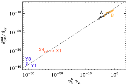
Figure 3: Dependence of ${\cal E}_{\rm GW}^{\rm sat}$ on $v_{\lambda}^{5}v_{\mu}$ for our runs of Series X (red) and Y (blue), as well as Series A (black) and B (orange) of Ref. Brandenburg:2021aln .

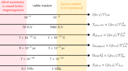
Figure 4: Summary of the viable parameter space for the hypercharge-weighted chiral chemical potential $\tilde{\mu}_{Y,5}$ and predictions for the relic magnetic field and gravitational wave radiation.

IV Conclusions

Our estimates of the key variables are summarized in Fig. 4. Since we assume Standard Model particles and interactions, as well as a standard cosmology with radiation domination at temperatures $T>100\ \mathrm{TeV}$, the observables depend only on the single dimensionless parameter $|\tilde{\mu}_{Y,5}|/T$, which controls the size of the initial hypercharge-weighted chiral asymmetry. To ensure that the instability develops before the chiral asymmetry is washed out by reactions such as Higgs decays and inverse decays, we need $|\tilde{\mu}_{Y,5}|/T\gtrsim 10^{-3}$. On the other hand, to avoid over-producing the baryon asymmetry we need $|\tilde{\mu}_{Y,5}|/T\lesssim 10^{-2}$. This leaves an approximately one-decade wide window of viable parameter space. The predicted magnetic field strength today, assuming inverse cascade scaling from production until recombination, is at the level of $10^{-15}\ \mathrm{Gauss}$. An intergalactic magnetic field at this level is barely strong enough to explain observations of distant TeV blazars, which provide evidence for a nonzero intergalactic magnetic field at the level $\gtrsim 10^{-16}\ \mathrm{Gauss}$ Neronov:2010gir . The same magnetic field may help to explain the origin of galactic magnetic fields by providing a seed for the galactic dynamo. The strength of the gravitational wave signal is expected to depend strongly on the value of $|\tilde{\mu}_{Y,5}|/T$, going as its sixth power. The typical frequency of this signal is expected to fall near $\sim\mathrm{GHz}$, putting it a frequency band that is being targeted by several recently proposed probes of high-frequency gravitational wave radiation. However, within the viable window, the gravitational wave signal is likely far too weak for detection.

Data availability—The source code used for the simulations of this study, the Pencil Code, is freely available from Ref. PC . The simulation setups and the corresponding data are freely available from Ref. DATA .

Acknowledgements—We thank Kohei Kamada, Sayan Mandal, and Jonathan Stepp for useful discussions and comments. A.J.L. is grateful to the Mainz Institute for Theoretical Physics (MITP) of the DFG Cluster of Excellence PRISMA+ (Project ID 39083149) as well as to the Aspen Center for Physics, which is supported by National Science Foundation grant PHY-2210452, for their hospitality during the completion of this work. Support through the NASA ATP award 80NSSC22K0825, the Swedish Research Council, grant 2019-04234, and Shota Rustaveli GNSF (grant FR/18-1462) are gratefully acknowledged. We acknowledge the allocation of computing resources provided by the Swedish National Allocations Committee at the Center for Parallel Computers at the Royal Institute of Technology in Stockholm. E.C. acknowledges the Pake Fellowship, and G.S. acknowledges support from the Undergraduate Research Office in the form of a Summer Undergraduate Research Fellowships (SURF) at Carnegie Mellon University.

References

- (1) E. W. Kolb and S. Wolfram, Nucl. Phys. B 172, 224 (1980), [Erratum: Nucl.Phys.B 195, 542 (1982)].
- (2) M. Fukugita and T. Yanagida, Phys. Lett. B174, 45 (1986).
- (3) G. Servant and S. Tulin, (2013), arXiv:1304.3464.
- (4) K. Dick, M. Lindner, M. Ratz, and D. Wright, Phys.Rev.Lett. 84, 4039 (2000), arXiv:hep-ph/9907562.
- (5) H. Murayama and A. Pierce, Phys. Rev. Lett. 89, 271601 (2002), arXiv:hep-ph/0206177.
- (6) B. A. Campbell, S. Davidson, J. R. Ellis, and K. A. Olive, Phys.Lett. B256, 484 (1991).
- (7) M. Joyce and M. E. Shaposhnikov, Phys.Rev.Lett. 79, 1193 (1997), arXiv:astro-ph/9703005.
- (8) Y. Akamatsu and N. Yamamoto, Phys. Rev. Lett. 111, 052002 (2013), arXiv:1302.2125.
- (9) A. Neronov and I. Vovk, Science 328, 73 (2010), arXiv:1006.3504.
- (10) T. Vachaspati, Rept. Prog. Phys. 84, 074901 (2021), arXiv:2010.10525.
- (11) D. V. Deryagin, D. Y. Grigoriev, V. A. Rubakov, and M. V. Sazhin, Mod. Phys. Lett. A 1, 593 (1986).
- (12) A. Brandenburg, Y. He, T. Kahniashvili, M. Rheinhardt, and J. Schober, Astrophys. J. 911, 110 (2021), arXiv:2101.08178.
- (13) M. M. Anber and L. Sorbo, Phys. Rev. D 81, 043534 (2010), arXiv:0908.4089.
- (14) N. Barnaby et al., Phys. Rev. D 86, 103508 (2012), arXiv:1206.6117.
- (15) V. Domcke, M. Pieroni, and P. Binétruy, JCAP 06, 031 (2016), arXiv:1603.01287.
- (16) C. S. Machado, W. Ratzinger, P. Schwaller, and B. A. Stefanek, JHEP 01, 053 (2019), arXiv:1811.01950.
- (17) A. Brandenburg, K. Kamada, and J. Schober, Phys. Rev. Res. 5, L022028 (2023), arXiv:2302.00512.
- (18) A. Brandenburg, K. Kamada, K. Mukaida, K. Schmitz, and J. Schober, (2023), arXiv:2304.06612.
- (19) J. S. Bell and R. Jackiw, Nuovo Cim. A 60, 47 (1969).
- (20) S. L. Adler, Phys. Rev. 177, 2426 (1969).
- (21) A. Vilenkin, Phys. Rev. D 22, 3080 (1980).
- (22) A. Boyarsky, J. Fröhlich, and O. Ruchayskiy, Phys. Rev. Lett. 108, 031301 (2012), arXiv:1109.3350.
- (23) A. Boyarsky, O. Ruchayskiy, and M. Shaposhnikov, Phys. Rev. Lett. 109, 111602 (2012), arXiv:1204.3604.
- (24) A. Boyarsky, J. Fröhlich, and O. Ruchayskiy, Phys. Rev. D 92, 043004 (2015), arXiv:1504.04854.
- (25) A. Brandenburg et al., Astrophys. J. Lett. 845, L21 (2017), arXiv:1707.03385.
- (26) K. Kamada, N. Yamamoto, and D.-L. Yang, Prog. Part. Nucl. Phys. 129, 104016 (2023), arXiv:2207.09184.
- (27) K. Kamada and A. J. Long, Phys. Rev. D 94, 063501 (2016), arXiv:1606.08891.
- (28) K. Kamada and A. J. Long, Phys. Rev. D 94, 123509 (2016), arXiv:1610.03074.
- (29) D. Bödeker and D. Schröder, JCAP 05, 010 (2019), arXiv:1902.07220.
- (30) M.-C. Chen, S. Ipek, and M. Ratz, Phys. Rev. D 100, 035011 (2019), arXiv:1903.06211.
- (31) T. Hatori, JPSJ 53, 2539 (1984).
- (32) G. Gogoberidze, T. Kahniashvili, and A. Kosowsky, Phys. Rev. D 76, 083002 (2007), arXiv:0705.1733.
- (33) A. Roper Pol, A. Brandenburg, T. Kahniashvili, A. Kosowsky, and S. Mandal, Geophys. Astrophys. Fluid Dynamics 114, 130 (2020), arXiv:1807.05479.
- (34) M. Maggiore, Phys. Rept. 331, 283 (2000), arXiv:gr-qc/9909001.
- (35) LIGO Scientific, Virgo, B. P. Abbott et al., Phys. Rev. Lett. 118, 121101 (2017), arXiv:1612.02029, [Erratum: Phys.Rev.Lett. 119, 029901 (2017)].
- (36) N. Bartolo et al., JCAP 11, 034 (2018), arXiv:1806.02819.
- (37) J. Baker et al., (2019), arXiv:1907.06482.
- (38) C. Caprini et al., JCAP 11, 017 (2019), arXiv:1906.09244.
- (39) D. J. Reardon et al., Astrophys. J. Lett. 951 (2023), arXiv:2306.16215.
- (40) J. Antoniadis et al., (2023), arXiv:2306.16214.
- (41) NANOGrav, A. Afzal et al., Astrophys. J. Lett. 951 (2023), arXiv:2306.16219.
- (42) H. Xu et al., Res. Astron. Astrophys. 23, 075024 (2023), arXiv:2306.16216.
- (43) B. Chandra Joshi et al., J. Astrophys. Astron. 43, 98 (2022), arXiv:2207.06461.
- (44) M. T. Miles et al., Mon. Not. Roy. Astron. Soc. 519, 3976 (2023), arXiv:2212.04648.
- (45) N. Aggarwal et al., Living Rev. Rel. 24, 4 (2021), arXiv:2011.12414.
- (46) T. Fujita and K. Kamada, Phys. Rev. D 93, 083520 (2016), arXiv:1602.02109.
- (47) M. Giovannini and M. E. Shaposhnikov, Phys. Rev. D 57, 2186 (1998), arXiv:hep-ph/9710234.
- (48) V. Domcke, K. Kamada, K. Mukaida, K. Schmitz, and M. Yamada, (2022), arXiv:2208.03237.
- (49) The pencil code. doi:10.5281/zenodo.2315093. https://github.com/pencil-code.
- (50) P. B. Arnold, G. D. Moore, and L. G. Yaffe, JHEP 11, 001 (2000), arXiv:hep-ph/0010177.
- (51) I. Rogachevskii et al., Astrophys. J. 846, 153 (2017), arXiv:1705.00378.
- (52) Pencil Code Collaboration, A. Brandenburg et al., J. Open Source Softw. 6, 2807 (2021), arXiv:2009.08231.
- (53) A. Brandenburg, Y. He, and R. Sharma, Astrophys. J. 922, 192 (2021), arXiv:2107.12333.
- (54) A. Roper Pol, S. Mandal, A. Brandenburg, T. Kahniashvili, and A. Kosowsky, Phys. Rev. D 102, 083512 (2020), arXiv:1903.08585.
- (55) A. Roper Pol, C. Caprini, A. Neronov, and D. Semikoz, Phys. Rev. D 105, 123502 (2022), arXiv:2201.05630.
- (56) R. Sharma and A. Brandenburg, Phys. Rev. D 106, 103536 (2022), arXiv:2206.00055.
- (57) A. Brandenburg, E. Clarke, T. Kahniashvili, A. J. Strong, and G. Sun, Datasets for Relic gravitational waves from the chiral plasma instability in the standard cosmological model, doi:10.5281/zenodo.8157463 (v2023.07.17); see also http://norlx65.nordita.org/~brandenb/proj/GWfromSM/ for easier access .