Primordial acoustic turbulence: three-dimensional simulations
and gravitational wave predictions

Abstract

Gravitational waves (GWs) generated by a first-order phase transition at the electroweak scale are detectable by future space-based detectors like LISA. The lifetime of the resulting shock waves plays an important role in determining the intensity of the generated GWs. We have simulated decaying primordial acoustic turbulence in three dimensions and make a prediction for the universal shape of the energy spectrum by using its self-similar decay properties and the shape of individual shock waves. The shape for the spectrum is used to determine the time dependence of the fluid kinetic energy and the energy containing length scale at late times. The inertial range power law is found to be close to the classically predicted $k^{-2}$ and approaches it with increasing Reynolds number. The resulting model for the velocity spectrum and its decay in time is combined with the sound shell model assumptions about the correlations of the velocity field to compute the GW power spectrum for flows that decay in less than the Hubble time. The decay is found to bring about a convergence in the spectral amplitude and the peak power law that leads to a power law shallower than the $k^{9}$ of the stationary case.

I Introduction

Gravitational waves (GWs) through their detection provide an exciting probe into the conditions of the early pre-recombination era universe that is beyond the reach of direct detection by electromagnetic radiation. Due to their weak interactivity, gravitational waves measured today carry near unfiltered information on the processes and conditions that led to their formation. One candidate for such a process are first-order phase transitions resulting from the electroweak symmetry breaking that are predicted by many beyond the Standard Model theories [1] that are motivated by explaining some of the model’s shortcoming, like the lack of a mechanism for baryogenesis. First-order transitions proceed by nucleation, growth, and merger of bubbles of the new phase [2, 3, 4, 5], and the produced GWs from the various resulting individual GW sources [6, 7, 8] form a stochastic gravitational wave background [9, 10] that could be within reach of future space-based GW detectors such as LISA [11].

A primordial, thermal first-order phase transition is likely to introduce a lot of kinetic energy into the primordial plasma, in the form of longitudinal or vortical motion. If the transition is strong enough, then the motion will become non-linear sufficiently quickly for there to be consequences for observation [12, 13]. This can even happen during the phase transition, with the generation of vorticity in the plasma and the potential formation of droplets [14, 15]. It is important therefore to both model the onset of such non-linearities and understand the resulting gravitational wave power spectrum as well as possible.

During a first-order phase transition energy is put in over a short period of time on a short range of length scales, leading to so-called freely decaying turbulence. Much attention has been paid to the development of vortical turbulence [16] – both forced and freely decaying – in the early universe and the consequences for gravitational waves [17, 18, 19]. However, for weak transitions and for strong detonations (transitions in which the bubble wall moves faster than the speed of sound in the plasma) the perturbations in the plasma are mostly longitudinal, corresponding to sound waves. Over time, these sound waves will steepen into shocks [20, 21]. The interactions in a random field of shocks lead to so-called acoustic turbulence [22, 23], and can act as an alternative mechanism for the dissipation of kinetic energy in a plasma.

There now exists extensive modelling [24, 25, 26, 27] and simulations [28, 29, 30, 31, 32] of the gravitational waves produced by acoustic waves in weak first-order thermal phase transitions, and notably the sound shell model [24, 25] shows good agreement with simulations of non-relativistic flows with length scales less than the Hubble scale [33]. In earlier works [34, 18, 19, 21, 35, 36], it has been shown that non-linearities of all kinds affect the efficiency of gravitational wave production. The goal of this paper is to study how acoustic turbulence forms in a hydrodynamical system inspired by early universe scenarios, through the use of numerical simulations.

In our previous work in Ref. [37] we simulated decaying acoustic turbulence in the simpler and more computationally efficient two-dimensional case. We studied the shape of the individual shocks and the fluid energy spectrum along with the decay properties of the system. Using the known universal properties of acoustic turbulence, we then extended the results to three dimensions and made an estimate on the GW power spectrum resulting from decaying acoustic turbulence based on the Sound Shell Model [25].

In this work we improve on the results by introducing additional previously missing terms into the fluid equations and by using more accurate higher order methods. We check the universal properties of acoustic turbulence by fits to the simulation data to determine how well they apply in the relativistic case. The dimensionally dependent results are also updated to the three-dimensional case, and we provide a more detailed analysis of the turbulence decay. Finally, the GW power spectrum computation is corrected based on recent findings.

The composition of this paper is as follows: In section II.1 we derive the fluid equations from the relativistic ones by assuming non-relatistic bulk velocities and the ultrarelativistic equation of state. We do not make any other assumptions about the energy density, and we take into account the spatial dependence of the dynamic viscosity, both of which lead to additional terms emerging compared to our earlier 2D study. In II.2 we discuss the methods and initial conditions used in the numerical simulations and introduce key quantities that are used in characterizing acoustic turbulence. We also introduce the velocity limiter that has been used in a few high Reynolds runs and the motivation behind it.

In III.1 the effects of the additional terms that emerged in the previous section are studied by numerical simulations. In III.2 the fluid equations are solved analytically for a single shock wave moving along the $x$-axis and expressions for the shock velocity and shock profile are obtained. The profile is used in III.3 to write the energy spectrum of decaying acoustic turbulence in a self-similar form by assuming it to be a broken power law modulated by a function depending on the shock width. Power laws in the spectrum are also measured by fitting and the obtained results are averaged in time over a suitable interval.

In III.4 the decay of kinetic energy is inspected and the time dependence of the kinetic energy and the integral length scale is derived at late times. The decay power law for the kinetic energy is extracted by fitting to the simulation data and is compared to the predicted value. We also briefly look at the generation of vorticity from irrotational initial conditions in section III.5.

Section IV studies the gravitational wave power spectrum that arises from shocks and acoustic turbulence using the properties of the energy spectrum and the found decay characteristics. The equations for the GW power spectrum are formulated for flows whose timescales are much less than the Hubble time at the time of the phase transition, meaning that the expansion of the universe can be neglected. The time evolution of the spectrum is then studied by numerical integration by approximating the decay of the flow based on the numerical simulations.

II Methods

II.1 Fluid equations

The fluid equations we have employed have been obtained from the relativistic fluid equations for non-perfect fluids by expanding them to second order in the case of non-relativistic bulk velocities $\mathbf{v}$ and small viscosities. When deriving the fluid equations in Ref. [37] we had assumed that the energy density consists of a background and perturbation, so that it has the form ${\rho(\mathbf{x},t)=\rho_{0}+\delta\rho(\mathbf{x},t)}$, where ${\delta\rho/\rho_{0}\ll 1}$. However, this assumption is not fulfilled everywhere in the fluid, as in the early times after the shocks have formed, the perturbation can grow large, and even substantially exceed the background value in regions containing strong shocks or many overlapping shock waves. Therefore, the terms that were discarded as a result of this assumption, would give non-negligible contributions in these regions, as they are proportional to the gradients of the logarithmic energy density. Hence, here we go through the derivation of the fluid equations, this time by not making any initial assumptions about the energy density. We have also been careful to include all terms up to second order in the expansions, and we end up with a new term in the continuity equation that is not present in Ref. [38]. We also properly take into account the spatial dependence of the dynamic viscosity, which gives new viscosity containing terms that would have also vanished under the previous assumptions of the energy density. The used units are such that velocities are given as fractions of the speed of light, i.e. $c=1$.

The relativistic fluid equations follow from

$$\nabla_{\nu}T^{\mu\nu}=0\,,$$ (1)

where in the absence of heat fluxes or external forcing, the energy-momentum tensor can be written in the form

$$T^{\mu\nu}=T^{\mu\nu}_{\text{PF}}+T^{\mu\nu}_{\text{NPF}}\,,$$ (2)

where the perfect fluid part is

$$T^{\mu\nu}_{\text{PF}}=(\rho+p)u^{\mu}u^{\nu}+pg^{\mu\nu}$$ (3)

and the non-perfect fluid part can be written as [39]

$$T^{\mu\nu}_{\text{NPF}}=-2\tilde{\eta}\sigma^{\mu\nu}\,.$$ (4)

Here $\mathbf{u}=\gamma(1,\mathbf{v})$ is the four-velocity, $p$ the pressure, $\rho$ the energy density, $g^{\mu\nu}$ the spacetime metric tensor, $\tilde{\eta}$ the dynamic shear viscosity, and

$$\sigma_{\mu\nu}=\nabla_{(\mu}u_{\nu)}+a_{(\mu}u_{\nu)}-\frac{1}{3}\theta h_{\mu\nu}$$ (5)

is the relativistic shear tensor. The parentheses denote the symmetric part of the tensor, $a^{\mu}=u^{\nu}\nabla_{\nu}u^{\mu}$ is the four-acceleration, ${\theta=\nabla_{\mu}u^{\mu}}$ the expansion scalar, and ${h_{\mu\nu}=g_{\mu\nu}+u_{\mu}u_{\nu}}$ the projection tensor. Here we have discarded the viscous bulk pressure term in the non-perfect fluid part of the energy-momentum tensor, since bulk viscosity is expected to be negligible in comparison to shear viscosity in relativistic plasmas [40]. In fluids dominated by irrotational modes, which is the case in this work, the shear and bulk viscosities also act in effectively the same way everywhere but in the vicinity of shock waves, meaning that the inclusion of the bulk viscosity would mostly only affect the magnitude of the effective viscosity parameter.

The components of the energy-momentum tensor are now expanded to second order while assuming all quantities and terms with the units of velocity to be small in comparison to the speed of light. We call such quantities first order small parameters and denote them by $\mathcal{O(\varepsilon)}$. For simplicity, we assume a time independent and uniform kinematic viscosity, denoted by $\eta$, which is related to the dynamic viscosity as $\tilde{\eta}(\mathbf{x})=\eta\rho(\mathbf{x})$. We employ the Minkowski metric $g^{\mu\nu}=\eta^{\mu\nu}=\text{diag}(-1,1,1,1)$ along with the ultrarelativistic equation of state $p=c_{s}^{2}\rho$, where $c_{s}$ is the speed of sound in the fluid, which for a radiation fluid obtains the value of $1/\sqrt{3}$. In flat spacetime the covariant derivatives simplify to $\nabla_{\mu}=\partial_{\mu}=(\partial_{t},\nabla)$, and the Lorentz factors expanded to second order become $\gamma^{2}=(1-v^{2})^{-1}=1+v^{2}+\mathcal{O}(\varepsilon^{4})$. The perfect fluid part of the energy-momentum tensor can then be written as

$$T^{00}_{\text{PF}} =\rho+(1+c_{s}^{2})\rho v^{2}+\mathcal{O}(\varepsilon^{4})$$ (6)

$$T^{0i}_{\text{PF}} =(1+c_{s}^{2})\rho v^{i}+\mathcal{O}(\varepsilon^{3})$$ (7)

$$T^{ij}_{\text{PF}} =(1+c_{s}^{2})\rho v^{i}v^{j}+\delta^{ij}c_{s}^{2}\rho+\mathcal{O}(\varepsilon^{4})\,,$$ (8)

and the non-perfect fluid part becomes

$$T^{00}_{\text{NPF}} =\mathcal{O}(\varepsilon^{3})$$ (9)

$$T^{0i}_{\text{NPF}} =\mathcal{O}(\varepsilon^{3})$$ (10)

$$T^{ij}_{\text{NPF}} =-2\tilde{\eta}S^{ij}+\mathcal{O}(\varepsilon^{3})\,,$$ (11)

where

$$S_{ij}=\frac{1}{2}\left(\frac{\partial v_{i}}{\partial x_{j}}+\frac{\partial v_{j}}{\partial x_{i}}-\frac{2}{3}\delta_{ij}\nabla\cdot\mathbf{v}\right)$$ (12)

is the traceless rate of shear tensor. The continuity equation is obtained from the $\mu=0$ component of Eq. (1), which after substituting the above expansions for the components of $T^{\mu\nu}$ can be written in the form

$$\frac{\partial\rho}{\partial t}+(1+c_{s}^{2})\nabla\cdot(\rho\mathbf{v})+(1+c_{s}^{2})\rho\frac{\partial v^{2}}{\partial t}+\mathcal{O}(\varepsilon^{3})=0\,.$$ (13)

Likewise, the Navier-Stokes equations follow from the $\mu=i$ components of the relativistic fluid equations, and unlike the continuity equation, pick up second order contributions from the non-perfect fluid part of the energy-momentum tensor, leading to emergence of viscosity containing terms. For the sake of clarity, we split the computation of the terms following from the perfect and non-perfect fluid parts. The terms following from the perfect fluid part on the left-hand side (LHS) of the equation are

$$\frac{\partial\mathbf{v}}{\partial t}+(\mathbf{v}\cdot\nabla)\mathbf{v}-c_{s}^{2}\mathbf{v}(\nabla\cdot\mathbf{v})-c_{s}^{2}\mathbf{v}(\mathbf{v}\cdot\nabla\ln\rho)\\ +\frac{c_{s}^{2}}{1+c_{s}^{2}}\nabla\ln\rho+\mathcal{O}(\varepsilon^{3})=\boldsymbol{\mathcal{N}}(\rho,\mathbf{v},\eta)\,,$$ (14)

where Eq. (13) has been used to replace a time derivative of the energy density, and to obtain this form, both sides of the equation have been divided be a factor of ${(1+c_{s}^{2})\rho}$. From this, $\partial_{t}v^{2}$ can be computed by taking the dot product from the left in terms of $\mathbf{v}$. Since we know that the viscosity dependent part $\boldsymbol{\mathcal{N}}(\rho,\mathbf{v},\eta)$ will be $\mathcal{O}(\varepsilon^{2})$, taking the dot product will give only third order contributions to the right-hand side (RHS). In fact, only the last term on the LHS of the equation will give a contribution that is less than third order small, leading to

$$\frac{\partial v^{2}}{\partial t}=-\frac{2c_{s}^{2}}{(1+c_{s}^{2})}\mathbf{v}\cdot\nabla\ln\rho+\mathcal{O}(\varepsilon^{3})\,.$$ (15)

Substituting this into the continuity equation (13) allows us to write it as

$$\frac{\partial\rho}{\partial t}+(1+c_{s}^{2})\nabla\cdot(\rho\mathbf{v})-2c_{s}^{2}\mathbf{v}\cdot\nabla\rho=0\,,$$ (16)

where the last term resulting from expanding the Lorentz factors gives a non-negligible contribution under the expansion used here. It was missing in our previous work in Ref. [37] and is also not present in Ref. [38] that deals with a similar limit.

The viscosity dependent part $\boldsymbol{\mathcal{N}}$ follows from

$$\mathcal{N}_{i}(\rho,\mathbf{v},\eta) =-\frac{1}{(1+c_{s}^{2})\rho}\partial_{j}T^{ij}_{\text{NPF}}$$

$$=\frac{2\eta}{(1+c_{s}^{2})\rho}\partial_{j}(\rho S_{ij})\,,$$ (17)

where the minus sign results from moving the terms in Eq. (1) to the RHS, and the factor following it from the division that was performed to obtain Eq. (14). After a straightforward calculation, $\boldsymbol{\mathcal{N}}$ can be written in a vector form as

$$\boldsymbol{\mathcal{N}}(\rho,\mathbf{v},\eta)=\frac{\eta}{1+c_{s}^{2}}\left[\nabla^{2}\mathbf{v}+\frac{1}{3}\nabla(\nabla\cdot\mathbf{v})+2\mathbf{S}\cdot\nabla\ln\rho\right]\,,$$ (18)

where we have used the notation $\mathbf{S}\cdot\nabla\ln\rho\equiv S_{ij}\partial_{j}\ln\rho$. Writing the continuity equation also in terms of the logarithmic energy density allows us to write the fluid equations up to second order in the form

$$\frac{\partial\ln\rho}{\partial t}+(1+c_{s}^{2})\nabla\cdot\mathbf{v}+(1-c_{s}^{2})\mathbf{v}\cdot\nabla\ln\rho=0$$ (19)

$$\frac{\partial\mathbf{v}}{\partial t}+(\mathbf{v}\cdot\nabla)\mathbf{v}-c_{s}^{2}\mathbf{v}(\nabla\cdot\mathbf{v})-c_{s}^{2}\mathbf{v}(\mathbf{v}\cdot\nabla\ln\rho)+\frac{c_{s}^{2}}{1+c_{s}^{2}}\nabla\ln\rho=\frac{\eta}{1+c_{s}^{2}}\left[\nabla^{2}\mathbf{v}+\frac{1}{3}\nabla(\nabla\cdot\mathbf{v})+2\mathbf{S}\cdot\nabla\ln\rho\right]\,.$$ (20)

Here the new terms compared to the fluid equations in Ref. [37] are the aforementioned term in the continuity equation, the new non-linear term that is second-to-last on the LHS of Eq. (20), and the last viscosity dependent shear rate tensor containing term on the RHS of the equation. We refer to these terms from now on by the name additional terms. The fluid equations above can be considered to describe relativistic fluids with non-relativistic bulk velocities in the limit of small viscosities.

II.2 Numerical simulations

We integrate the fluid equations (19) and (20) numerically in three dimensions using a Python code that builds on the two-dimensional simulation code used in Ref. [37]. The spatial derivatives are computed using a sixth order central finite difference scheme [41, 42], and second order cross derivatives are evaluated using an approximate bidiagonal scheme [43] that is faster than applying the individual derivatives consecutively. The simulation grid is a cube of size $N^{3}$ with unit spacing so that ${\Delta x=\Delta y=\Delta z=1.0}$, and periodic boundary conditions are applied on all sides. The reciprocal lattice is given in terms of wavevectors $\mathbf{k}_{i}$ with spacing $\Delta k_{x}=2\pi/(N\Delta x)$ obtaining values in the interval $k_{i}\in[-\pi,\pi)$. The time integration is carried out using the fourth order Runge-Kutta scheme with an adaptive time step. We fix the Courant number of the flow $\mathcal{C}$ to the value of 0.5, which gives a well converging solution, and vary the size of the time step based on the maximum velocity present in the flow at any given time through the equation

$$\Delta t=\frac{\mathcal{C}\Delta x}{u}\,,\quad u=\frac{c_{s}+|\mathbf{v}|_{\text{max}}}{1+c_{s}|\mathbf{v}|_{\text{max}}}\,.$$ (21)

The quantities advanced at each time step are the velocity components $v_{i}$ and the logarithmic density $\ln\rho$.

In this work we do not simulate the phase transition that precedes acoustic turbulence in order to save computation time, and to ensure that the observed effects are not special to phase transitions. Instead, the initial conditions are given in terms of the rotational (transverse) and irrotational (longitudinal) velocity components $\mathbf{v}_{\perp}$ and $\mathbf{v}_{\parallel}$ that satisfy

$$\mathbf{v}=\mathbf{v}_{\parallel}+\mathbf{v}_{\perp}$$ (22)

$$\nabla\cdot\textbf{v}_{\perp}=0\,,\quad\nabla\times\textbf{v}_{\parallel}=0\,.$$ (23)

The transverse component is initialized to be zero, so that the flow is initially completely longitudinal and produces acoustic turbulence after a single shock formation time

$$t_{s}=\frac{L_{0}}{\bar{v}_{0}}\,,$$ (24)

which is the timescale associated with the non-linearities in the flow. Here $\bar{v}_{0}$ is the initial value of the root mean square (rms) velocity of the flow $\bar{v}=\sqrt{\left\langle\mathbf{v}^{2}\right\rangle}$, and $L_{0}$ is the initial value of the integral length scale, defined in Eq. (30), which characterizes the energy containing length scale of the flow. A fluid initialized from irrotational initial conditions is dominated by the longitudinal quantities at all times, and therefore we do not make a distinction between the total and the longitudinal quantities in notation, as they are the same to a very high degree of accuracy.

The longitudinal velocity component is initialized by giving the initial spectral density $P(k)$ defined through

$$\left\langle v_{i}(\mathbf{k})v_{i}(\mathbf{k}^{\prime})\right\rangle=(2\pi)^{3}P(k)\delta(\mathbf{k}-\mathbf{k}^{\prime})$$ (25)

as a broken power law with an exponential suppression of the form

$$P(k)=A\frac{(k/k_{p})^{\xi}}{\left[1+(k/k_{p})^{\alpha/\delta}\right]^{\delta}}e^{-(k/k_{d})^{2}}\,.$$ (26)

Here $k_{p}$ is the wavenumber that sets the peak of the spectrum, $\xi$ is the power law index of the low-$k$ power law that appears below the peak, and the parameter $\alpha$ sets the high-$k$ power law that follows the peak with the power law index $\xi-\alpha$. The extent of this power law range is controlled by the parameter $k_{d}$, which controls where the exponential suppression becomes significant. It is given a value of $k_{d}=1/\sqrt{5}\approx 0.447$ in all runs featured in this paper. Finally, the parameter $\delta$ controls the sharpness of the peak. The Fourier components of the longitudinal velocity are computed from the spectral density and are given random complex phases. The components are then Fourier inverse transformed using the convention

$$v_{i}(\mathbf{k}) =\int v_{i}(\mathbf{r})e^{-i\mathbf{r}\cdot\mathbf{k}}\,d^{3}r$$ (27)

$$v_{i}(\mathbf{r}) =\frac{1}{(2\pi)^{3}}\int v_{i}(\mathbf{k})e^{i\mathbf{r}\cdot\mathbf{k}}\,d^{3}k$$ (28)

to obtain the corresponding real space velocity components. The random phases given to the Fourier components generate random initial conditions after the inverse transform. The initial background density is uniform with a value of ${\rho_{0}=1.0}$ in all cases. For more information about the simulation code and the initial conditions, see Appendix C.

An energy spectrum $E(k)$ describing the distribution of kinetic energy across the length scales in the flow is defined as

$$\left\langle\mathbf{v}^{2}\right\rangle=\int\limits_{0}^{\infty}E(k)\,dk\,,\quad E(k)=\frac{k^{2}}{2\pi^{2}}P(k)\,.$$ (29)

We denote the low-k power law in the energy spectrum by $\beta$, which means that it relates to the power law in the spectral density as $\beta=\xi+2$. The high-$k$ power law in the energy spectrum is then $\beta-\alpha$, which often in the context of vortical turbulence is called the inertial range power law, which we also adopt here. The integral length scale $L$ is related to the energy spectrum through the equation

$$L=\frac{1}{\bar{v}^{2}}\int\limits_{0}^{\infty}\frac{1}{k}E(k)\,dk\,.$$ (30)

Two other length scales characterizing turbulence, that also work analogously in the acoustic case, are the Kolmogorov length scale

$$L_{K}=\left(\frac{\mu^{3}}{\epsilon}\right)^{1/4}\,,$$ (31)

which gives the length scale at which viscosity dominates, and the Taylor microscale

$$L_{T}=\sqrt{\frac{\bar{v}^{2}}{\left\langle(\nabla\cdot\textbf{v})^{2}\right\rangle}}\,,$$ (32)

which is an intermediate length scale below which viscous effects start to become significant. In Eq. (31) the quantity denoted by $\epsilon$ is the viscous dissipation rate of the longitudinal kinetic energy, given by

$$\epsilon=\frac{\mu}{1+c_{s}^{2}}\int\limits_{0}^{\infty}k^{2}E(k)\,dk\,.$$ (33)

The quantity $\mu$ is the effective viscosity in the irrotational case, which has the value of $\mu=4\eta/3$. This follows from the first two terms on the RHS of Eq. (20) having the same form when ${\nabla\times\mathbf{v}=0}$, and assuming that the final term gives on average only third order small contributions, since $\nabla\ln\rho$ can be assumed to be $\mathcal{O}(\varepsilon)$ outside shocks and shock collisions, which only account to a small fraction of the total fluid volume. The effective viscosity and the rms velocity can be combined to yield a quantity with dimensions of length

$$\delta_{s}\sim\frac{\mu}{\bar{v}}\,,$$ (34)

which characterizes the width of the shocks in the flow. We also define the quantity

$$\text{Re}=\frac{\bar{v}L}{\mu}\,,$$ (35)

which, analogously to the Reynolds number of vortical turbulence, gives the strength of the non-linear effects in the flow (i.e. shocks in the irrotational case).

The inclusion of the additional terms, the utilized higher order methods, and the increase in dimensions limits the range of obtainable Reynolds numbers compared to the two-dimensional case due to instabilities appearing at points where multiple strong shocks collide, which can grow and ruin the numerical solution in a very short time frame. To combat this phenomenon we employ a velocity limiter that suppresses all velocity values that exceed a certain threshold value. This allows us to reach the kind of Reynolds numbers that were present in Ref. [37]. The mechanism behind the limiter is as follows: If the value of the velocity exceeds some threshold value $v_{t}$ at any point in any of the velocity components $v_{i}$, the value is suppressed towards $v_{t}$ at that point by multiplying it by a factor $s$. The value of the logarithmic energy density at the corresponding grid point is also suppressed by this factor towards the mean logarithmic energy density. This is necessary because at the divergence point both the velocity and the energy density grow large, and one of them drives the other. The velocity limiter is activated after each time the state of the fluid is updated in the simulations. In terms of equations, it can be formulated as follows: For velocities $|v_{i}|\geq v_{t}$ in the arrays

$$v_{i}=\begin{cases}v_{t}+s\left|v_{i}-v_{t}\right|&\text{if}\ v_{i}\geq 0\\ -v_{t}-s\left|v_{i}+v_{t}\right|&\text{if}\ v_{i}<0\end{cases}$$ (36)

and the for the corresponding logarithmic energy density values at the same site as the $v_{i}$ scaling was done

$$\ln\rho=\begin{cases}\ln\rho_{0}+s\left|\ln\rho-\ln\rho_{0}\right|&\text{if}\ \ln\rho\geq\ln\rho_{0}\\ \ln\rho_{0}-s\left|\ln\rho-\ln\rho_{0}\right|&\text{if}\ \ln\rho<\ln\rho_{0}\,.\end{cases}$$ (37)

The desired effect is, that by fine-tuning the threshold velocity $v_{t}$, the velocity limiter prevents the non-physical divergence in the fluid but only affects the shock collisions, where the largest velocities in the fluid are obtained, but which only amount to a very small percentage of the total volume. We also activate the limiter only at times larger than a single shock formation time so that it does not affect the shock formation. If the affected volume is small enough, the velocity limiter should not have a noticeable effect on the quantities that are of interest to us, like the energy decay rates or the shape of the energy spectrum. Additionally, if the largest values in the flow are obtained at the non-physical oscillations at the crest of the shocks that follow from discretization effects induced when the numerical scheme tries to handle sharp discontinuities, the velocity limiter should not have much effect on the physical properties of the system. Based on our tests, a threshold value of $v_{t}=0.5$ provides a good balance. The other parameter to be set is the suppression strength $s$. The suppression should be smooth enough to minimize any imprints on the fluid, while being strong enough to still prevent a divergence from occurring. We have used a value of $s=0.5$ in our velocity limiter runs (those being XIII, XIV, and XV of Table 9), which is found to satisfy the aforementioned conditions. The effects of the velocity limiter are inspected in Appendix A by comparing two runs with the same initial fluid state but with one of them using the limiter. There we find that the limiter mostly impacts rotational quantities and has a minimal effect on longitudinal quantities and spectral indices.

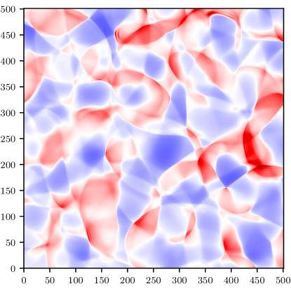
(a)

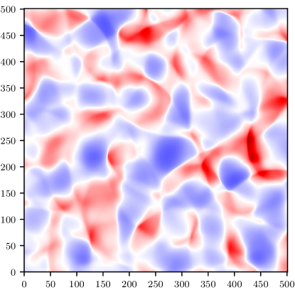
(b)

Figure 1: A zoom in of the non-uniform energy density $\delta\rho$ slice in Run V at $t\approx 2.5t_{s}$. Both plots use the same normalization for the color scheme, red regions corresponding to positive values, blue regions to negative ones, and regions close to zero are white. In Figure (a) the additional terms in equations (19) and (20) are disabled, corresponding to the fluid equations in Ref. [37]. Figure (b) contains the energy density with all terms included, displaying the smoothing effect around the shock waves resulting from these terms.

III Results

We have studied the decay of three-dimensional acoustic turbulence by performing numerical simulations with grid sizes of $1000^{3}$. The irrotational initial conditions we have employed are generated from a diverse group of initial energy spectra resulting from Eq. (26) with various different initial power laws. The initial Reynolds numbers in the runs range from 10 to 190, and the velocity limiter detailed in section III.1 has been used in the high Reynolds number runs to prevent a non-physical divergence in the velocity values that can occur when strong shocks collide. The duration of the runs is about 20 shock formation times, which is long enough to display sufficient decay characteristics and to extract information about the decay. The runs and the initial conditions are listed in Table 9 of Appendix C. In this section we study the changes to the results found in Ref. [37] that follow from moving to 3D and employing the additional terms in the fluid equations.

III.1 Effects of the additional terms

The additional terms that emerge in equations (19) and (20) can be divided into two groups. One of them contains the new first order small term in the continuity equation (16), and in the other group there are the new second order small terms in Eq. (20) that are all proportional to $\nabla\ln\rho$, which would have been neglected in Ref. [37] due to being third order small. However, these terms are expected to give non-negligible contributions in regions where the gradients of the logarithmic energy density are not small, which can occur in the vicinity of shock waves.

For comparison, we have conducted an alternate version of Run V that has exactly the same initial state as the original run, but the additional terms in the fluid equations are disabled. We have compared these two runs to study how the additional terms affect the flows. Figure 1 shows a portion of a two-dimensional slice of the non-uniform energy density component $\delta\rho$ soon after shocks have formed. In Figure 1a the additional terms have been disabled, and wavelike patterns can be clearly seen trailing the shock waves. These result from the oscillations at the crest of the shock waves (see, for example, Figure 2a in Ref. [37]) that are discretization effects that follow from the used numerical scheme’s inability to properly handle sharp discontinuities. The steeper the shocks, the stronger these oscillations are, until for steep enough shocks the oscillations start diverging, ruining the numerical solution. This limits the range of obtainable Reynolds numbers for the numerical simulations. The velocity can also obtain large values locally at these oscillations. Figure 1b shows the energy density at the same time with all terms in (19) and (20) enabled. The additional terms smooth out the regions around the shock waves, as the oscillations are far less prominent. This effect is also seen in Figure 2, which shows the maximum value of the velocity in the flow for the two runs as a function of the number of shock formation times.

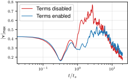
Figure 2: The maximum velocity in the flow for Run V as a function of the number of shock formation times. The red curve shows the value in the case where the additional terms are disabled, and the blue curve in the case where all terms are included. The smoothing effect of the additional terms is seen here at initial times when the shocks are at their strongest, as the maximum velocity in this range is substantially smaller when the terms are enabled.

The largest velocity in the flow soon after shock formation is substantially smaller when the additional terms are enabled, indicating a smoothing out of the flow due to reduction in the oscillations trailing shock waves. As mentioned at the start of this section, we expect the change around the shocks to be attributed to the effect of the latter group of new terms that are proportional to $\nabla\ln\rho$.

The other group of terms in the continuity equation breaks the classical form of the continuity equation and thus under the expansion used to obtain the fluid equations, leads to third order small violations to the conservation of non-relativistic energy $\left\langle\rho(\mathbf{x})\right\rangle=\rho_{0}$, which is seen in Figure 3 that plots the mean energy density against time.

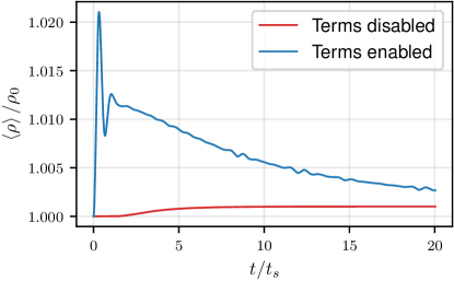
Figure 3: The mean energy density as a function of the number of shock formation times in Run V. The red curve shows the value in the case where the additional terms are disabled, and the blue curve in the case where all terms are included. While the energy density is no longer conserved as well as before as a result of the new term that emerges in the continuity equation, the deviation from the mean value still remains small and approaches the initial mean value over time after the initial stage.

The energy density deviates from the initial mean value as the shocks form, but the magnitude of the deviation remains small. After the shocks have formed, the deviation gets smaller over time and the energy density approaches the initial mean value. As such, we do not expect this to have any kind of adverse effects on the validity of the results presented in this paper.

The effect that the additional terms have on the kinetic energy decay and the energy spectrum are also relevant questions for the topic of this paper. The kinetic energy $\mathcal{E}=\left\langle\mathbf{v}^{2}\right\rangle/2$ as a function of the number of shock formation times is plotted in Figure 5. While the kinetic energy starts decaying a bit slower with the additional terms included, the actual dissipation rate of the kinetic energy remains the same at late times, as can be seen from the power laws at times $t\geq 10t_{s}$. There is a change in the decay rate at early times, which results from the change in shock shape detailed in section III.2, which affects the value of the decay constant $C$ introduced in section III.4. Similar behavior is seen in the integral length scales shown in Figure 5, where there is a small difference in the values after shock formation, the same power law is still seen after ten shock formation times. For transverse quantities, especially for the transverse kinetic energy $\mathcal{E}_{\perp}=\left\langle\mathbf{v}^{2}_{\perp}\right\rangle/2$, the differences between the two cases are more notable. With the additional terms included, the amount of generated transverse kinetic energy is larger by an order of magnitude at the end of the simulation, indicating a stronger vorticity generation when the new terms are included. Nevertheless, the vorticity still remains small at all times and as a result, so do the transverse quantities when compared with the longitudinal ones. Vorticity generation from irrotational initial conditions is inspected more closely in section III.5.

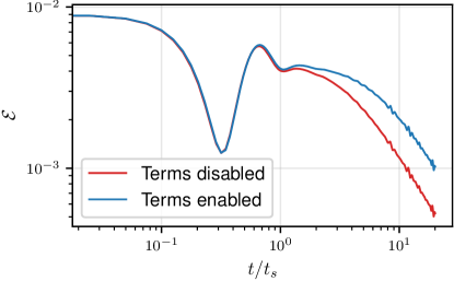
Figure 4: The total kinetic energy as a function of the number of shock formation times in Run V. With the additional terms included, the kinetic energy decays more slowly after the shocks form, but both curves still follow the same decay power law after $t>10t_{s}$.

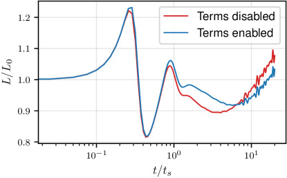
Figure 5: The integral length scale as a function of the number of shock formation times in Run V. After the initial phase when the shocks form, its value ends up being initially slightly larger with the additional terms included, but both curves still follow the power law after $t>10t_{s}$.

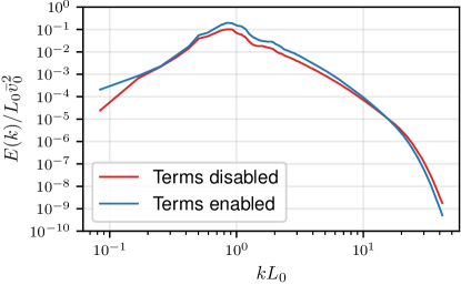
Figure 6: The energy spectrum $E(k)$ in Run V at $t\approx 15t_{s}$. The additional terms do not have an effect on the power law values at low wavenumbers or at the inertial range. Instead, they only affect the spectral amplitude due to the difference between the kinetic energies in Figure 5, and the shape of the spectrum at the very high-$k$ end.

Figure 6 shows the effect of the additional fluid equation terms to the total energy spectrum of the fluid at $t=15t_{s}$. The difference in the amount of kinetic energy is seen as a small deviation in the amplitudes of the spectra. However, it can be seen that there is no change in the low-$k$ power law that lies roughly in the range $0.2\leq kL_{0}\leq 0.6$, nor in the inertial range power law at $1.0\leq kL_{0}\leq 2.0$. A clear difference in the shape of the spectrum can be seen at high wavenumbers at length scales where the viscous dissipation is considerable. In Ref. [37] the shape of the high-$k$ end of the spectrum was attributed to the shape and steepness of the shock waves in the flow. This indicates that the additional terms lead to a change in the shock shape compared to what was found in [37]. We study this change next in section III.2. To conclude, the additional terms do not change the relevant power laws that are under study in this work, which also allows for comparison to the results found in the 2D case.

III.2 Shock shape with the additional terms

In this section we repeat the calculation found in section IIIA of our previous work in Ref. [37] that studies two-dimensional acoustic turbulence, but now with the additional terms included in the fluid equations. We consider a single right moving shock with the ansatz

$$\ln\rho(\mathbf{x},t) =L(k_{s}(x-u_{s}t))$$ (38)

$$\mathbf{v}(\mathbf{x},t) =V(k_{s}(x-u_{s}t))\hat{\mathbf{e}}_{x}$$ (39)

and expand the equations to second order using the same kind of expansion as in section II.1. We also assume that the shock velocity $u_{s}$ is much larger than the velocities appearing in the flow, so that $V/u_{s}\ll 1$. Denoting $y\equiv k_{s}(x-u_{s}t)$ and substituting the ansatzes into the continuity equation, the result up to second order can be written in the form

$$\frac{dL(y)}{dy}=\frac{1+c_{s}^{2}}{u_{s}}\left[1+(1-c_{s}^{2})\frac{V(y)}{u_{s}}\right]\frac{dV(y)}{dy}+\mathcal{O}(\varepsilon^{3})\,.$$ (40)

Here we have picked up a non-vanishing contribution from the new additional term in the continuity equation. From this we can also note that since at its lowest order the derivative of $L(y)$ is proportional to the derivative of $V(y)$, then $dL(y)/dy$ is also a first order small quantity. This means that the term that results from the new additional non-linear term on the LHS of Eq. (20) is third order small and vanishes. Substituting the ansatzes to equation (20) and expanding gives

$$\left[(1-c_{s}^{2})V(y)-u_{s}\right]\frac{dV(y)}{dy}+\frac{c_{s}^{2}}{1+c_{s}^{2}}\frac{dL(y)}{dy}=\\ \frac{\mu k_{s}}{1+c_{s}^{2}}\left(\frac{d^{2}V(y)}{dy^{2}}+\frac{dV(y)}{dy}\frac{dL(y)}{dy}\right)+\mathcal{O}(\varepsilon^{3})\,,$$ (41)

where $\mu=4\eta/3$ is the effective viscosity. Here the last viscosity dependent term on the RHS follows from the new additional terms that contain the shear rate tensor, and we can see that it also vanishes, being third order small. After substituting Eq. (40) into this and rearranging, the differential equation for $V(y)$ up to second order becomes

$$\frac{d^{2}V(y)}{dy^{2}}+\frac{1}{\mu k_{s}}\left[a+bV(y)\right]\frac{dV(y)}{dy}=0\,,$$ (42)

which is of the same form that was obtained without the additional terms, but with different coefficients, those now being

$$a =u_{s}(1+c_{s}^{2})\left(1-\frac{c_{s}^{2}}{u_{s}^{2}}\right)$$ (43)

$$b =(c_{s}^{4}-1)\left(1+\frac{c_{s}^{2}}{u_{s}^{2}}\right)\,.$$ (44)

The boundary conditions for the shock wave are

$$V(+\infty) =V_{+}$$ (45)

$$V(-\infty) =V_{-}$$ (46)

$$\frac{dV(y)}{dy}\Bigg{|}_{y=\pm\infty} =0$$ (47)

meaning that the value on the LHS of the shock is $V_{-}$, and $V_{+}$ on the RHS, and the velocity is a constant either side of the shock. The differential equation (42) is simple to solve with these boundary conditions, which results in the equation

$$C_{s}\equiv aV_{-}+\frac{b}{2}V_{-}^{2}=aV_{+}+\frac{b}{2}V_{+}^{2}\,.$$ (48)

Using Eqs. (43) and (44), this becomes an equation for the shock velocity $u_{s}$

$$u_{s}^{3}-c_{s}^{2}u_{s}+\frac{1}{2}(c_{s}^{2}-1)(u_{s}^{2}+c_{s}^{2})(V_{-}+V_{+})=0\,,$$ (49)

from which $u_{s}$ can be solved when the values on the left and right side of the shock are known. The solution to the differential equation is

$$V(x,t)=\frac{\sqrt{a^{2}+2bC_{s}}}{b}\tanh\left[k_{s}(x-x_{0}-u_{s}t)\right]-\frac{a}{b}\,,$$ (50)

where

$$k_{s}=\frac{\sqrt{a^{2}+2bC_{s}}}{2\mu}$$ (51)

is a parameter whose inverse describes shock width, which has now changed from the previous one in Ref. [37] because of the change in parameters $a$ and $b$. The equation in the earlier paper also had a typo, where the factor was written in terms of the shear viscosity $\eta$, giving a factor 4/3, but the effective viscosity $\mu$ was still used in the notation.

From the continuity equation, we can also solve $L(y)$ and the energy density $\rho$ by using the result for $V(y)$. This gives

$$\rho(x,t)=\frac{\rho_{0}}{\left[1-\frac{1-c_{s}^{2}}{u_{s}}V(x,t)\right]^{\frac{1+c_{s}^{2}}{1-c_{s}^{2}}}}\,.$$ (52)

Writing the energy density as

$$\rho(x,t)=\rho_{0}+\delta\rho(x,t)\,,$$ (53)

where $\delta\rho$ is the non-uniform part, and assuming ${V/u_{s}\ll 1}$, the result becomes

$$V(x,t)\approx\frac{u_{s}}{1+c_{s}^{2}}\widetilde{\delta\rho}(x,t)\,,\quad\widetilde{\delta\rho}(x,t)=\frac{\delta\rho(x,t)}{\rho_{0}}.$$ (54)

Using this to write the shock velocity equation (49) in terms of the energy density instead of the velocity makes the cubic equation quadratic, giving us the following approximate result for $u_{s}$:

$$u_{s}\approx c_{s}\sqrt{\frac{2(1+c_{s}^{2})+(1-c_{s}^{2})(\widetilde{\delta\rho}_{+}+\widetilde{\delta\rho}_{-})}{2(1+c_{s}^{2})-(1-c_{s}^{2})(\widetilde{\delta\rho}_{+}+\widetilde{\delta\rho}_{-})}}\,,$$ (55)

which clearly shows the fact that the shock velocity is always larger than the speed of sound in the fluid, and that it gets larger with increasing shock height.

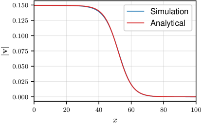
Figure 7: A right moving shock in a shock tube run at early times. The blue curve is the simulation data, and the red curve is the analytical prediction for the shock shape using equations (43)-(51). The values used for the analytical prediction are $\eta=0.4$, $V_{-}=0.149$, $V_{+}=0.0$, and $x_{0}=51.9$, resulting in a shock velocity ${u_{s}\approx 0.625\approx 1.083c_{s}}$.

We have verified the results found in this section by conducting a run in a narrow shock tube of size 10000x4x4, which very closely corresponds to a one-dimensional situation. The shear viscosity parameter has been chosen to be quite large at $\eta=0.4$ to eliminate the discretization effects that follow from sharp features. The initial velocity is taken to be zero everywhere, and the non-uniform part of the energy density is of the form

$$\delta\rho(x)=\frac{1}{2}\left[\tanh\left(\frac{1}{4}\left(x+\frac{N}{20}\right)\right)\right.\\ \left.-\tanh\left(\frac{1}{4}\left(x-\frac{N}{20}\right)\right)\right]\,,$$ (56)

that with $N=10000$ gives an initial state that corresponds to a square wave around the origin. At the start of the simulation it breaks into a right- and a left-moving shock wave. The right-moving shock has been plotted in Figure 7 in blue. Also plotted, as a red line, is the prediction for the shock wave with parameter values $\eta=0.4$, $V_{+}=0.149$, $V_{-}=0.0$, and $x_{0}=51.9$. The figure shows that the simulation data and the analytical prediction are in an excellent agreement with each other.

III.3 Shocks and the energy spectrum in three dimensions

It is well established for acoustic turbulence in the case of the classical Burgers’ and Navier-Stokes equations that around the peak the spectrum obtains a universal broken power law form after shock formation regardless of the initial conditions, with a characteristic $k^{-2}$ power law at the inertial range that was first proposed by Burgers [44] in one dimensions and later generalized to multiple dimensions by Kadomtsev and Petviashvili [45], which is why it is also sometimes referred to as the KP spectrum. Assuming that the inertial range behavior is cut off at a length scale where viscous effects start to become notable, we can write

$$E(k)=A_{E}\frac{(k/k_{p})^{\beta}}{1+(k/k_{p})^{\alpha}}\,,\quad k\ll 1/L_{T}\,,$$ (57)

where $\beta-\alpha=-2$ according to the KP result. The spectral amplitude $A_{E}$ can be related to the parameters of the flow and the initial spectrum by using the definition of the energy spectrum in Eq. (29), and the definition of the integral length scale in Eq. (30). The integrals present in the equations obtain their largest contributions around the peak, so for spectra with long enough inertial ranges (i.e. high Reynolds numbers), the high wavenumber behavior of the spectrum can be ignored. Then substituting Eq. (57) into (30) gives

$$k_{p}L\equiv\kappa_{p}\approx\frac{\sin\left[\frac{\pi(\beta+1)}{\alpha}\right]}{\sin\left(\frac{\pi\beta}{\alpha}\right)}\,,$$ (58)

and using this in the result obtained in the same way from Eq. (29) gives

$$A_{E}\approx\bar{v}^{2}L\frac{\alpha}{\pi}\sin\left(\frac{\pi\beta}{\alpha}\right)\,.$$ (59)

Using this, the energy spectrum can be written as

$$E(\kappa,t)=L(t)\mathcal{E}(t)\Psi(\kappa)\,,\quad\kappa=L(t)k\,,$$ (60)

where $\mathcal{E}=\left\langle\mathbf{v}^{2}\right\rangle/2$ is the kinetic energy, and $\Psi(\kappa)$ is defined as a broken power law function of the form

$$\Psi(\kappa)=\Psi_{0}\frac{(\kappa/\kappa_{p})^{\beta}}{1+(\kappa/\kappa_{p})^{\alpha}}\,,\quad\kappa\ll L/L_{T}$$ (61)

with

$$\Psi_{0}\approx\frac{2\alpha}{\pi}\sin\left(\frac{\pi\beta}{\alpha}\right)\,.$$ (62)

Since the power laws in the spectrum remain the same over time, $\kappa_{p}$ and $\Psi_{0}$ can be treated as constants in time. Writing the spectrum like this extracts the time dependence of the spectral amplitude and fixes the location of the peak in $\kappa$-space, making the spectra at different times collapse into each other in the wavenumber range that follows the broken power law form when the spectral shape function $\Psi(\kappa)$ is plotted, as can be seen in Figures 4 and 5 of Ref. [37] in the two-dimensional case. The figure shows that at length scales smaller than the Taylor microscale, the spectral shape function $\Psi(\kappa)$ still has time dependence, which in that Ref. was associated with the change in the shape of the shock waves caused by the viscous dissipation. Therefore, it was suggested, that $\Psi$ is a broken power law modulated by a function that is dependent on the shock width. Finding the modulating function depends on the dimensionality of the system, meaning that the calculation needs to be repeated here in the three-dimensional case.

The starting point is to compute the one-dimensional energy spectrum using the shape of the shock waves found in the previous section

$$E_{1}(k)=|\mathcal{F}(\tanh(k_{s}x))|^{2}=\frac{\pi^{2}}{k_{s}^{2}}\text{csch}^{2}\left(\frac{\pi k}{2k_{s}}\right)\,,$$ (63)

where $\mathcal{F}$ denotes the Fourier transform. The $D$-dimensional spectrum can be computed from this via the equation

$$E_{1}(k_{1})=\frac{1}{2}\Omega_{D-1}\int\limits_{k_{1}^{2}}^{\infty}E_{D}(s)(s^{2}-k_{1}^{2})^{\frac{D-3}{2}}\,ds^{2}\,,$$ (64)

which has been obtained by integrating the $D$-dimensional spectrum over the wavevector components perpendicular to $\mathbf{k}_{1}$. In three dimensions the equation ends up being simpler than in 2D, giving with Eq. (63) the relation

$$\int\limits_{k_{1}}^{\infty}sE_{3}(s)\,ds=\frac{\pi}{2k_{s}^{2}}\text{csch}^{2}\left(\frac{\pi k_{1}}{2k_{s}}\right)\,.$$ (65)

The 3D spectrum $E_{3}(k)$ that satisfies the above integral equation is

$$E_{3}(k)=\frac{\pi^{2}}{2k_{s}^{3}k}\frac{\cosh\left(\frac{\pi k}{2k_{s}}\right)}{\sinh^{3}\left(\frac{\pi k}{2k_{s}}\right)}\,.$$ (66)

Scaling out the constants by defining

$$E_{3}=\frac{\pi^{3}}{4k_{s}^{4}}\mathcal{I}\,,\quad P=\frac{\pi k}{2k_{s}}$$ (67)

gives the modulating function $\mathcal{I}$ as

$$\mathcal{I}(P)=\frac{1}{P}\frac{\cosh(P)}{\sinh^{3}(P)}\sim\begin{cases}\dfrac{1}{P^{4}}\,,\quad P\ll 1\\ \dfrac{4}{P}e^{-2P}\,,\quad P\gg 1\,.\end{cases}$$ (68)

The spectral shape function $\Psi(\kappa)$ is then

$$\Psi(\kappa)=\widetilde{\Psi}_{0}\frac{(\kappa/\kappa_{p})^{\beta+4}}{1+(\kappa/\kappa_{p})^{\alpha}}\mathcal{I}\left(\frac{\pi\kappa}{2\kappa_{s}}\right)\,,$$ (69)

where the low wavenumber behavior of the modulating function has been taken into account so that $\beta$ still denotes the low-$k$ power law value of the energy spectrum, giving the relation

$$\widetilde{\Psi}_{0}=\left(\frac{\pi\kappa_{p}}{2\kappa_{s}}\right)^{4}\Psi_{0}\,.$$ (70)

We have tested the validity of the obtained spectral shape by using Eq. (69) as a fitting function to the simulation data. The function $\Psi$ can be obtained from the energy spectrum data through Eq. (60). A fit to the data of Run I at the end of the run (i.e. after 20 shock formation times) has been plotted in Figure 8.

Figure 8: Fit (dashed red line) on the function $\Psi(\kappa)$ obtained from the longitudinal energy spectrum data of Run I at ${t=20t_{s}}$ using Eq. (69) as the fitting function. The obtained fit parameters are $\widetilde{\Psi}_{0}=0.61$, $\beta=3.31$, $\alpha=7.72$, $\kappa_{p}=1.03$, and $\kappa_{s}=2.65$.

The lower limit of the fit is $kL=0.3$ and the upper limit is unbounded. For this low Reynolds number run the spectral shape function of Eq. (69) fits the simulation data very well. As the Reynolds number increases, the fits get slightly worse because of effects like the numerical oscillations at the shocks and the bottleneck effect [46, 47], both of which deform the spectrum at high wavenumbers, deteriorating the fit. Regardless, the correspondence between the fit and the simulation data remains good even in our highest Reynolds number runs. Table 1 shows the fitting results for the spectral indices and the integral length scale scaled inverse shock width $\kappa_{s}$ for each of the runs.

ID	Re	$\beta$	$\alpha$	$\kappa_{s}$
I	$3.66$	$3.31$	$7.72$	$2.65$
II	$10.51$	$1.53$	$5.50$	$7.30$
III	$8.72$	$3.10$	$6.88$	$5.87$
IV	$13.54$	$3.61$	$6.80$	$8.63$
V	$11.75$	$4.70$	$7.85$	$7.37$
VI	$16.41$	$3.87$	$6.81$	$9.88$
VII	$19.32$	$5.28$	$8.04$	$11.12$
VIII	$22.54$	$3.77$	$6.71$	$15.30$
IX	$29.42$	$1.43$	$4.43$	$21.22$
X	$27.30$	$4.23$	$6.96$	$16.39$
XI	$31.75$	$3.63$	$6.35$	$19.50$
XII	$43.47$	$1.61$	$4.32$	$25.82$
XIII	$49.83$	$3.19$	$5.70$	$33.13$
XIV	$69.91$	$1.37$	$3.90$	$38.16$
XV	$58.18$	$3.24$	$5.69$	$35.83$

Table 1: The fit parameters $\beta$, $\alpha$, and $\kappa_{s}$ for all runs using Eq. (69) as a fitting function to the $\Psi(\kappa)$ data from the simulations at $t=20t_{s}$ (see Fig. 8). Also listed is the Reynolds number of the run at the time of the fit. Figure 9 shows the correlation between it and the shock width parameter $\kappa_{s}$ using the above values.

The fitting errors in the $\kappa_{s}$ parameter are of the order $\mathcal{O}(10^{-2})$. Also listed are the Reynolds numbers at the fitting time. There is a clear trend between them and the $\kappa_{s}$ values, which is being illustrated in Figure 9.

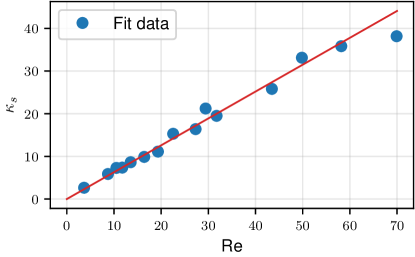
Figure 9: The fitting results for the parameter $\kappa_{s}$ of Eq. 69 listed in Table 1 plotted against the Reynolds number at the fitting time. The red line is a linear fit $\kappa_{s}=d\text{Re}$ with ${d=0.630\pm 0.014}$.

The data points imply a direct proportionality, that in the figure has been indicated by a red line with a slope of $d=0.630\pm 0.014$ obtained by a linear fit. Using the definitions of $\kappa_{s}$ and the Reynolds number in Eq. (35), this results in

$$\kappa_{s}=k_{s}L=d\text{Re}=d\frac{\bar{v}L}{\mu}$$ (71)

$$\Rightarrow k_{s}=d\frac{\bar{v}}{\mu}\,.$$ (72)

The shock width follows from this directly as

$$\delta_{s}=\frac{1}{k_{s}}=\frac{1}{d}\frac{\mu}{\bar{v}}\approx 1.588\frac{\mu}{\bar{v}}\,,$$ (73)

meaning that the obtained fitting parameters are in a good agreement with the shock width length scale of Eq. (34). This shows that the high wavenumber behavior of the energy spectrum is indeed modulated by the shock width, and that the argument of the modulating function (68) can be directly related to the shock width length scale at the given time.

The fits in Table 1 give approximate results for the power law indices of the energy spectrum but are not ideal for a number of reasons. Since the fits include also the high wavenumbers beyond the inertial range, the high Reynolds number effects that deform the spectrum described in the previous paragraph worsen the fit and lead to a higher error in the obtained values for the spectral indices. The grid sizes we have used lead to there being only a few data points between the smallest wavenumber ($\Delta k$) and the peak of the spectrum, especially at late times, when the integral length scale has grown and the peak of the spectrum has shifted towards larger scales. This lack of dynamic range coupled with a fixed lower fitting range limit of $kL=0.3$ results to there not being enough of the low-$k$ power law range to obtain accurate measurements in some cases, or the lower limit ends up being too close to the peak, which results in a small value for $\beta$ (around 1.5) for some runs.

In order to obtain more accurate results for the power law indices $\alpha$ and $\beta$, we employ the fitting strategy used in our previous work in [37], where a simple broken power law function

$$E_{\parallel}(k)=D\frac{\left(k/k_{p}\right)^{\beta}}{1+\left(k/k_{p}\right)^{\alpha}}$$ (74)

is used as the fitting function., so that $\beta$ gives the low wavenumber power law, and $\beta-\alpha$ the power law at the inertial range. We take the fitting range to be unbounded from below and $2/3L_{k}$ from above, and to measure temporal fluctuations in the fits, we average the obtained fit parameters in the range $9\leq t/t_{s}\leq 11$, which on average leads to around 80 fits per run. The choice of the averaging range to be quite late, and not earlier when the shocks are at their strongest, is to minimize the effect of the oscillations that appear at low wavenumbers around the peak of the spectrum. These oscillations are generated by the discrete Fourier transforms as a result of steep features appearing in the flow when the initial conditions gradually steepen into shocks, disturbing the fits. In the chosen time range the oscillations have already mostly died down, while still being early enough feature strong shocks and show a clear inertial range.

ID	$\beta_{0}$	$\beta_{0}-\alpha_{0}$	$\left\langle\beta\right\rangle_{t}$	$\sigma_{\beta}$	$\left\langle\alpha\right\rangle_{t}$	$\sigma_{\alpha}$	$\left\langle\beta-\alpha\right\rangle_{t}$	$\sigma_{\beta-\alpha}$
I	$5$	$-7$	$4.053$	$0.032$	$7.173$	$0.194$	$-3.120$	$0.213$
II	$4$	$-2$	$3.074$	$0.411$	$5.240$	$0.303$	$-2.165$	$0.124$
III	$4$	$-8$	$3.400$	$0.326$	$6.321$	$0.221$	$-2.920$	$0.125$
IV	$5$	$-4$	$3.959$	$0.181$	$6.442$	$0.185$	$-2.483$	$0.018$
V	$6$	$-14$	$4.270$	$0.187$	$6.875$	$0.192$	$-2.605$	$0.024$
VI	$6$	$-4$	$4.356$	$0.172$	$6.819$	$0.175$	$-2.463$	$0.013$
VII	$7$	$-19$	$4.384$	$0.432$	$6.766$	$0.428$	$-2.382$	$0.017$
VIII	$10$	$-5$	$4.178$	$0.541$	$6.572$	$0.509$	$-2.394$	$0.061$
IX	$3$	$-8$	$2.668$	$1.345$	$4.998$	$1.251$	$-2.330$	$0.102$
X	$5$	$-15$	$3.715$	$0.724$	$6.048$	$0.695$	$-2.333$	$0.043$
XI	$4$	$-12$	$3.184$	$0.908$	$5.521$	$0.865$	$-2.338$	$0.051$
XII	$2$	$-19$	$1.575$	$0.792$	$3.924$	$0.772$	$-2.349$	$0.034$
XIII	$3$	$-29$	$3.638$	$1.493$	$5.858$	$1.463$	$-2.220$	$0.050$
XIV	$2$	$-31$	$1.934$	$1.387$	$4.160$	$1.361$	$-2.227$	$0.034$
XV	$4$	$-48$	$3.231$	$1.120$	$5.439$	$1.105$	$-2.208$	$0.037$

Table 2: The initial low-$k$ power law of the energy spectrum $\beta_{0}$ and the initial inertial range power law $\beta_{0}-\alpha_{0}$, and the same power laws after the shocks have formed obtained by time averaging the results from the broken power law fits of Equation (74) over the interval $9\leq t/t_{s}\leq 11$. Also listed are the standard deviations for the time fluctuations for each of the parameters.

Table 2 lists the initial power laws in the spectrum along with the time averaged power laws and the standard deviations resulting from the time averaging. It clearly shows that the power laws in the initial spectrum have no effect on the power laws that are present in the spectrum after shock formation, leading to a universal spectrum for acoustic turbulence. The numerical values for the low-$k$ power law $\beta$ are in general steeper than what was found in the two-dimensional case in Ref. [37]. The standard deviations are larger in the high Reynolds number runs due to the shortness of the power law range. The most precise measurement with the lowest standard deviation is provided by Run I, which has the peak initially at a wavenumber that is much larger than in any of the other runs, giving a long range for measuring the $k^{\beta}$ power law. The values for the time averaged inertial range power laws are a bit steeper than the KP result $k^{-2}$ that is expected for classical Navier-Stokes. They do however display a clear tendency towards such a value with increasing Reynolds number. Here the measurements get more precise with increasing Reynolds number because the inertial range gets longer and easier to measure. The measurements along with the standard deviations from the time fluctuations have been plotted in Figure 10.

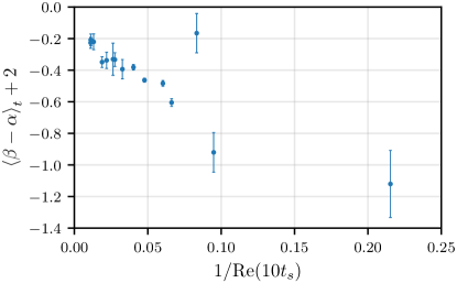
Figure 10: The scaled inertial range power law values $\left\langle\beta-\alpha\right\rangle_{t}$ of Table 2 plotted against the Reynolds number at the middle of the averaging interval at $t=10t_{s}$. The standard deviations resulting from the time fluctuations are shown as error bars for each case.

However, more data points at higher Reynolds numbers are needed to determine whether the power law converges towards the value of -2, or something slightly steeper, with the kind of fluid equations used here. Some runs also have a dip in the spectrum in the inertial range, like in Run V, as seen in Figure 6, that affects the measured power law values. At the high wavenumber end of the dip there is also a small bump in the spectrum, whose location corresponds to the Taylor microscale. The reason for this phenomenon that was not present in our previous 2D simulations requires more study.

We have also checked that the standard deviations resulting from the fitting covariances are small compared to the standard deviations of the time averaging for all parameters listed in Table 2.

III.4 Decay of kinetic energy for acoustic turbulence

III.4.1 Differential equation for the kinetic energy

Since the fluid equations we have employed do not feature a forcing term, the kinetic energy of the fluid decays into heat over time due to the viscous dissipation. The equation describing the change of the kinetic energy $\mathcal{E}=\left\langle\mathbf{v}^{2}\right\rangle/2$ over time can be obtained from Eq. (20) by taking a dot product with respect to the velocity and volume averaging both sides of the equation. In the volume averages gradients of the logarithmic energy density can be treated as first order small quantities, since they give significant contributions only at the shock waves, which constitute only a small part of the total volume. Then the last term on the RHS, and the second to last term on the LHS of the resulting equation are of the order $\mathcal{O}(\varepsilon^{4})$ (using the notation of section II.1), and are negligible compared to the other terms. Assuming irrotational case ($\nabla\times\mathbf{v}=0$), the equation can be written as

$$\frac{1}{2}\frac{\partial\left\langle\mathbf{v}^{2}\right\rangle}{\partial t}+\left\langle\mathbf{v}\cdot(\mathbf{v}\cdot\nabla)\mathbf{v}\right\rangle-c_{s}^{2}\left\langle v^{2}(\nabla\cdot\mathbf{v})\right\rangle\\ +\frac{c_{s}^{2}}{1+c_{s}^{2}}\left\langle\mathbf{v}\cdot\nabla\ln\rho\right\rangle=\frac{\mu}{1+c_{s}^{2}}\left\langle\mathbf{v}\cdot\nabla^{2}\mathbf{v}\right\rangle+\mathcal{O}(\epsilon^{4})$$ (75)

where $\mu=4\eta/3$. The first non-linear term and the pressure gradient term can be written as

$$\left\langle\mathbf{v}\cdot(\mathbf{v}\cdot\nabla)\mathbf{v}\right\rangle =\frac{1}{2}\left\langle\nabla\cdot(v^{2}\mathbf{v})\right\rangle-\frac{1}{2}\left\langle v^{2}(\nabla\cdot\mathbf{v})\right\rangle$$ (76)

$$\left\langle\mathbf{v}\cdot\nabla\ln\rho\right\rangle =\left\langle\nabla\cdot(\mathbf{v}\ln\rho)\right\rangle-\left\langle(\nabla\cdot\mathbf{v})\ln\rho\right\rangle$$ (77)

where the first terms on the RHS yield zero after writing the volume integrals as surface integrals using the divergence theorem and imposing that the velocity vanishes at the infinite boundary. The differential equation for the kinetic energy then becomes

$$\frac{1}{2}\frac{\partial\left\langle\mathbf{v}^{2}\right\rangle}{\partial t}=\frac{\mu}{1+c_{s}^{2}}\left\langle\mathbf{v}\cdot\nabla^{2}\mathbf{v}\right\rangle+\frac{c_{s}^{2}}{1+c_{s}^{2}}\left\langle(\nabla\cdot\mathbf{v})\ln\rho\right\rangle\\ +\left(c_{s}^{2}+\frac{1}{2}\right)\left\langle v^{2}(\nabla\cdot\mathbf{v})\right\rangle+\mathcal{O}(\epsilon^{4})\,,$$ (78)

where the first term is the viscous dissipation, the second term results from the pressure gradient term, and the last term from the non-linear terms in the fluid equations. From this it can be seen that in the vortical case the last two terms vanish and only the viscous dissipation term contributes to the time evolution of the kinetic energy, which is why in the literature about vortical turbulence only the first term is considered. However, in the case of acoustic turbulence the terms should not be neglected, and we find that they are comparable to the viscous dissipation at early times after shock formation.

In order to study the decay more closely, we have computed the magnitude of the three terms on the RHS of Equation (78) in Run VII. The results are plotted in Figure 11 as a function of the number of shock formation times along with the total dissipation rate of the kinetic energy fraction $\mathcal{E}_{r}(t)=\mathcal{E}(t)/\mathcal{E}_{0}$ (dashed black line).

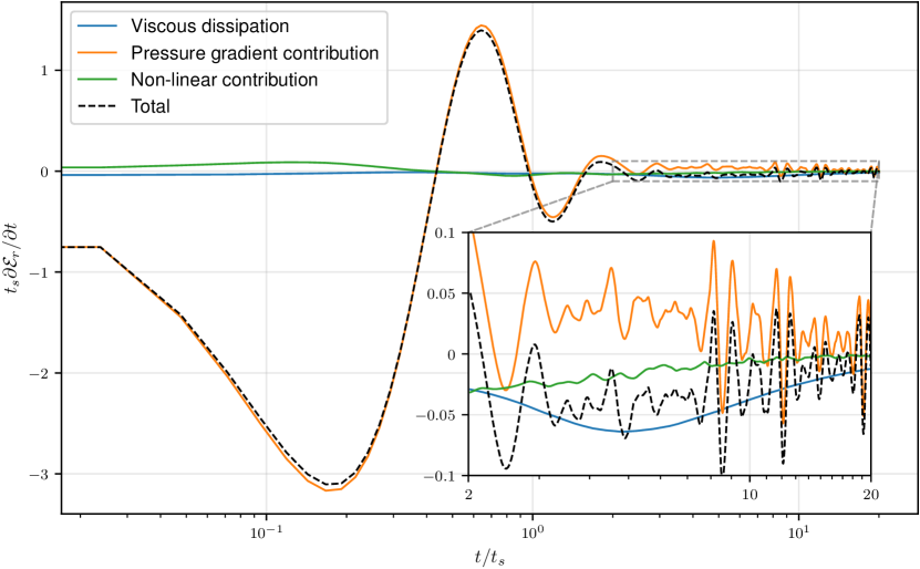
Figure 11: The dissipation rate of the kinetic energy fraction $\mathcal{E}_{r}(t)=\mathcal{E}(t)/\mathcal{E}_{0}$ resulting from the viscous dissipation, the pressure gradient, and the non-linear contributions of Equation (78) measured in Run VII. At early times before the shocks form, the steepening of the initial conditions into shocks causes strong oscillation in the pressure gradient contribution. After shock formation, the pressure gradient term is positive and generates kinetic energy, while the other two contributions dissipate it. At late times the viscous dissipation becomes the dominant term and sets the mean decay rate while the pressure gradient contribution induces oscillations into it.

The blue curve is the viscous dissipation (first term), the orange curve is the dissipation term resulting from the pressure gradient term in the fluid equations (second term), and the green curve is the contribution from the non-linear terms (third term). In Figure 78 we have also plotted the kinetic energy fraction of the same run obtained from simulation data along with the fraction obtained by integrating Eq. (11) numerically with the fourth order Runge-Kutta scheme using the measured total decay rate.

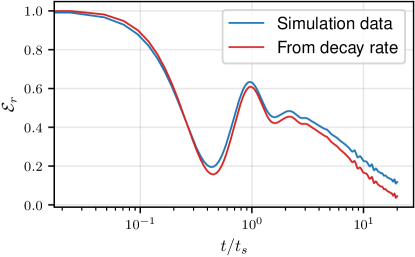
Figure 12: The kinetic energy fraction of Run VII obtained from simulation data (blue curve) plotted with the fraction (red curve) computed from the measured values of the terms of the energy dissipation equation (78), also visualized in Figure 11.

They are in a good agreement, with the remaining deviations explained by the fourth order terms that were neglected in deriving the kinetic energy evolution equation. As the initial conditions steepen into shocks, strong oscillations appear in the pressure gradient contribution that have a negative sign initially and strongly dissipate the kinetic energy. This is seen in the kinetic energy as a sharp drop, that in the case of Run VII leads to about 80% of the initial kinetic energy being dissipated by $t\approx 0.5t_{s}$. The oscillations remain strong until about $2t_{s}$, during which the pressure gradient term is the dominant one and clearly dictates the shape of the kinetic energy curve. At $t>2t_{s}$ the oscillations settle down and the pressure gradient contribution (on average) has a positive sign, transforming internal energy into kinetic energy. The contribution resulting from the non-linear terms only effectively affects the total decay rate soon after the shocks form by dissipating kinetic energy, becoming small and approaching zero at $t>10t_{s}$. The viscous dissipation term is negative at all times, reaching a minimum around $t=5t_{s}$, after which is starts increasing and approaching zero. It approaches zero slower than the pressure gradient term on average, meaning that at $t>10t_{s}$ it approximately sets the mean decay rate, while the pressure gradient contribution induces oscillations into it. This means that the behavior of the kinetic energy at late times, and the decay power law seen, for example, in Figure 5, can be extracted by studying the viscous dissipation term.

III.4.2 Kinetic energy at late times

We studied the decay of the kinetic energy in 2D acoustic turbulence in our previous work in Ref. [37] but did not provide the full picture of the decay, for the pressure gradient and non-linear contributions to the time evolution of the kinetic energy were ignored like in the case of vortical turbulence. The viscous dissipation term was also calculated using a method in a paper by Saffman in Ref. [48] and applying it analogously to the non-vortical case to solve the differential equation for the kinetic energy analytically. However, this is not necessary, and $\mathcal{E}(t)$ can be solved in a more natural way by using the actual energy spectrum of Equation (60). In this section we provide a more detailed calculation of the kinetic energy with the full spectrum, using the spectral shape function of Equation (69).

At late times, when the mean decay rate is set by the viscous dissipation rate, we can write

$$\frac{1}{2}\frac{\partial\left\langle\mathbf{v}^{2}\right\rangle}{\partial t}\approx\frac{\mu}{1+c_{s}^{2}}\left\langle\mathbf{v}\cdot\nabla^{2}\mathbf{v}\right\rangle=-\frac{\mu}{1+c_{s}^{2}}\int\limits_{0}^{\infty}k^{2}E(k)\,dk$$ (79)

where the integral form is obtained by Fourier transforming the RHS and using the definitions for the spectral density $P(k)$ and the energy spectrum $E(k)$. The spectrum is now approximated by splitting it into three pieces. We extend the low-$k$ power law all the way to the peak wavenumber $k_{p}$, after which the spectrum is assumed to have the characteristic $k^{-2}$ inertial range behavior. It is approximated that the modulation by shocks kicks in at the wavenumber corresponding to the shock width length scale. Then, using Equations (60), (68), and (69), the approximation reads as

$$E(k)\approx\begin{cases}\dfrac{L^{\beta+1}\mathcal{E}\Psi_{0}}{\kappa_{p}^{\beta}}k^{\beta}&k<k_{p}\\[10.76385pt] \dfrac{\mathcal{E}\Psi_{0}\kappa_{p}^{2}}{L}\frac{1}{k^{2}}&k_{p}\leq k\leq\delta_{s}^{-1}\\[10.76385pt] \dfrac{\mathcal{E}\Psi_{0}\kappa_{p}^{2}}{L}\left(\frac{\pi}{2}\right)^{3}\delta_{s}^{3}k\frac{\cosh\left(\pi\delta_{s}k/2\right)}{\sinh^{3}\left(\pi\delta_{s}k/2\right)}&k>\delta_{s}^{-1}\end{cases}$$ (80)

This leads to an overestimation around the peak of the spectrum in the integral of Eq. (79), which is negligible for high Reynolds number runs due to the $k^{2}$ scaling in the integrand. The decay rate is also overestimated somewhat at high wavenumbers because the actual spectrum has already started to fall off by the inverse shock width wavenumber, unlike assumed here. The result for the integral can now be written as

$$\int\limits_{0}^{\infty}k^{2}E(k)\,dk=\mathcal{E}\Psi_{0}\kappa_{p}^{2}\left(\mathcal{A}\frac{\delta_{s}^{-1}}{L}-\frac{\beta+2}{\beta+3}\frac{\kappa_{p}}{L^{2}}\right)\,,$$ (81)

where

$$\mathcal{A}=1+\frac{2}{\pi}\int\limits_{\pi/2}^{\infty}x^{3}\frac{\cosh x}{\sinh^{3}x}\,dx\approx 1.62\,.$$ (82)

Since the spectrum does not change over time on small wavenumbers, the kinetic energy $\mathcal{E}(t)$ and the integral length scale $L(t)$ are related as

$$\mathcal{E}L^{\beta+1}=\text{const.}$$ (83)

This can be used to replace the integral length scale in order to obtain a differential equation for the kinetic energy only. Using the result for the integral in Eq. (81), the relation above, and the result for the shock width in Eq. (73) allows us to write the differential equation (79) for the kinetic energy fraction $\mathcal{E}_{r}(t)=\mathcal{E}(t)/\mathcal{E}_{0}$ in the form

$$\frac{d\mathcal{E}_{r}}{dt}=-B\left(\mathcal{E}_{r}^{\frac{3\beta+5}{2(\beta+1)}}-D\mathcal{E}_{r}^{\frac{\beta+3}{\beta+1}}\right)$$ (84)

with the coefficients

$$B =\mathcal{A}d\frac{\Psi_{0}\kappa_{p}^{2}}{1+c_{s}^{2}}\frac{1}{t_{s}}$$ (85)

$$D =\frac{\kappa_{p}}{\mathcal{A}d}\frac{\beta+2}{\beta+3}\frac{1}{\text{Re}_{0}}\,,$$ (86)

where $\text{Re}_{0}$ is the initial Reynolds number, and $t_{s}$ is the non-linearity timescale of Eq.(24), and $d$ is the proportionality constant in the shock width relation of Eq. 72. The solution of the differential equation can be written as

$$\mathcal{E}_{r}(t)^{-\frac{\beta+3}{2(\beta+1)}}{}_{2}F_{1}\left(1,\frac{\beta+3}{\beta-1};\frac{2(\beta+1)}{\beta-1};D\mathcal{E}_{r}(t)^{\frac{1-\beta}{2(\beta+1)}}\right)\\ =C\frac{t}{t_{s}}+C^{\prime}$$ (87)

where ${}_{2}F_{1}$ is the hypergeometric function, $C^{\prime}$ an integration constant, and

$$C=\frac{\mathcal{A}d}{2}\frac{\beta+3}{\beta+1}\frac{\Psi_{0}\kappa_{p}^{2}}{1+c_{s}^{2}}\,.$$ (88)

The function ${}_{2}F_{1}$ can be written as a hypergeometric series that is close to unity when

$$\frac{\mathcal{E}(t)}{\mathcal{E}_{0}}\gg\left(\frac{\kappa_{p}}{\mathcal{A}d}\frac{\beta+2}{\beta+3}\frac{1}{\text{Re}_{0}}\right)^{\frac{2(\beta+1)}{\beta-1}}$$ (89)

or in terms of the integral length scale

$$\frac{L(t)}{L_{0}}\ll\left(\frac{\mathcal{A}d}{\kappa_{p}}\frac{\beta+3}{\beta+2}\text{Re}_{0}\right)^{\frac{2}{\beta-1}}\,.$$ (90)

This means that at very late times when the inertial range has shortened enough, the contributions from the peak of the spectrum to the viscous dissipation integral can no longer be neglected, and the solution becomes modulated by a hypergeometric function of this form. The kinetic energy fraction that this depends on is set by the initial Reynolds number of the flow, i.e. the initial length of the inertial range. In the case of $\beta=4$ and $d=0.63$, for the lowest Reynolds number run of this paper with $\text{Re}_{0}=10$ these become

$$\frac{\mathcal{E}(t)}{\mathcal{E}_{0}}\gg 1.1\cdot 10^{-8}\,,\quad\frac{L(t)}{L_{0}}\ll 7.3$$ (91)

which are well fulfilled in our simulation runs that last only 20 shock formation times, meaning that we do not expect the modulating behavior to have an effect on the power laws seen in the simulations. At the range of times when the hypergeometric function can be approximated to unity, the solution with the initial condition $\mathcal{E}(0)=\mathcal{E}_{0}$ can be written as

$$\mathcal{E}(t)=\frac{\mathcal{E}_{0}}{\left(1+C\frac{t}{t_{s}}\right)^{\zeta}}\,,\quad\zeta=\frac{2(\beta+1)}{\beta+3}\,,$$ (92)

and using the relation between the kinetic energy and the integral length scale in Eq. (83) gives

$$L(t)=L_{0}\left(1+C\frac{t}{t_{s}}\right)^{\lambda}\,,\quad\lambda=\frac{2}{\beta+3}\,.$$ (93)

Here we have now denoted the kinetic energy decay power law by $\zeta$, and the power law at which the integral length scale increases by $\lambda$. These same results were also found in our 2D study in Ref. [37], derived using the Saffman spectrum. The calculation is based on the universal properties of the acoustic turbulence spectrum having a $k^{-2}$ power law at the inertial range, and the spectrum being stationary at low wavenumbers, giving the same functional form for the kinetic energy in all dimensions. These power law values are only seen at late times ($t>10t_{s}$) when the pressure gradient and non-linear term contributions to the energy dissipation rate have died down. This also leads to a slower decay than what would be expected by just the viscous dissipation term due to the positivity of the pressure gradient contribution. This is why the value for $C$ in Eq. (88) differs from the ones seen in the simulations. It is also affected by factors that were not taken into account in deriving the spectral shape earlier, like the bottleneck phenomenon at large wavenumbers. The relations in Eqs. (92) and (93) can be used to derive relations between the power law indices $\beta$, $\zeta$ and $\lambda$:

$$\lambda(\beta+1)-\zeta =0$$ (94)

$$\zeta-2(1-\lambda) =0\,,$$ (95)

and also results for the time behavior of quantities like the Reynolds number, shock width length scale, and the Kolmogorov length scale using Eqs. (33) and (81).

III.4.3 Fits to the simulation data

Using Eq. (92) as a fitting function to the simulation data can be used to extract numerical values for the decay power laws $\zeta$, and the decay constants $C$. Time averaging has been introduced by varying the lower boundary of the fitting range in the interval $10\leq t/t_{s}\leq 13$, and averaging over the obtained parameter values. In this range the dissipation of kinetic energy is dominated by the viscous dissipation term and the results of the previous section should be approximately valid. The fits have been carried out fitting to the kinetic energy fraction $\mathcal{E}_{r}(t)$, leaving $\zeta$ and $C$ as the fitting parameters. The value for the decay constant $C$ obtained this way can be thought of as an effective $C$ that would hold if the decay seen in the simulation data took place following the functional form found in the previous section already from the beginning.

The results for these fitting parameters are listed in Table 3 along with their standard deviations for each of the featured runs. Also listed are the expected values for the energy decay power law resulting from the relation in Eq. (92) using the measured values of $\left\langle\beta\right\rangle_{t}$ listed in Table 2. The uncertainty in the value results from the standard deviations $\sigma_{\beta}$.

ID	$\left\langle\zeta\right\rangle_{t}$	$\sigma_{\zeta}$	$\zeta$	$\left\langle C\right\rangle_{t}$	$\sigma_{C}$
I	$1.497$	$0.019$	$1.433\pm 0.003$	$0.240$	$0.006$
II	$0.891$	$0.016$	$1.341\pm 0.045$	$0.517$	$0.023$
III	$1.257$	$0.014$	$1.375\pm 0.032$	$0.243$	$0.005$
IV	$1.172$	$0.022$	$1.425\pm 0.015$	$0.257$	$0.010$
V	$1.447$	$0.019$	$1.450\pm 0.014$	$0.177$	$0.004$
VI	$1.313$	$0.022$	$1.456\pm 0.013$	$0.206$	$0.006$
VII	$1.438$	$0.028$	$1.458\pm 0.032$	$0.176$	$0.006$
VIII	$1.258$	$0.028$	$1.443\pm 0.042$	$0.204$	$0.009$
IX	$1.059$	$0.031$	$1.294\pm 0.167$	$0.289$	$0.019$
X	$1.318$	$0.034$	$1.404\pm 0.064$	$0.193$	$0.010$
XI	$1.283$	$0.029$	$1.353\pm 0.095$	$0.201$	$0.009$
XII	$1.317$	$0.043$	$1.126\pm 0.151$	$0.200$	$0.013$
XIII	$1.448$	$0.074$	$1.397\pm 0.136$	$0.169$	$0.016$
XIV	$1.402$	$0.101$	$1.189\pm 0.228$	$0.186$	$0.026$
XV	$1.359$	$0.100$	$1.358\pm 0.115$	$0.198$	$0.028$

Table 3: Time averaged fit parameters for the kinetic energy power laws $\zeta$, obtained by fitting the function of Eq. (92) to the kinetic energy data and varying the lower boundary of the fit in the range $10\leq t/t_{s}\leq 13$. Also listed are the standard deviations, and the predicted values for the power laws given by equations(92) obtained by using the time averaged low-$k$ power law values $\left\langle\beta\right\rangle_{t}$ found in Table 2.

The values obtained for the time averaged power law index $\left\langle\zeta\right\rangle_{t}$ are in general a bit steeper than those found in 2D, as expected, due to the steeper low-$k$ power law that is present in the three-dimensional case. The predicted values for $\zeta$ are close to the values obtained from fitting, and within the errors resulting from time fluctuations for about half of the runs, and close for the majority of the remaining runs, with a few outliers like Run II, for whose abnormal values we have no explanation at the time of writing. The obtained values for the effective decay constant $C$ are somewhat smaller than what was found in 2D, where they obtained values in the range between 0.29 and 0.47. The constant $C$ sets the number of shock formation times it takes for the fluid to start decaying, with small values leading to slower decay. Since the decay was found to be slower with the additional terms included in Figure 5 of section III.1, the change in the measured values for the parameter $C$ here and in our previous 2D study can be attributed to the addition of the new terms into the fluid equations. While the additional terms do not change the functional form of $\mathcal{E}(t)$, they do lead to a change in the shock shape as seen in section III.2. This changes the shock width length scale $\delta_{s}$, and thus the shape of the spectrum at large wavenumbers through the modulating function (69). Since the additional terms lead to only fourth order small contributions in the energy decay rate equation (75), that should not affect the decay rate significantly, as also supported by Figure 11, the change in the value of $C$ between the two cases should follow mostly from the aforementioned effect.

We have opted not to include measurements of the integral length scale power law $\lambda$ or the relations in Equations (94) and (95). Due to the lack of dynamic range, the peak of the energy spectrum ends up being close to the lowest wavenumber $\Delta k=2\pi/N$ in the simulations, and gets closer over time as the integral length scale increases. The values at the low wavenumber end in the energy spectrum fluctuate over time, which leads to fluctuations in the peak, which is seen as oscillations in the measured $L(t)$ curve. This makes it difficult to extract the power law value accurately by fitting, especially in the high Reynolds number runs where low-$k$ power law range is short and the fluctuations are strong. We also see a decrease in the integral length scale after the shocks form that lasts for a few shock formation times that was not present in our 2D simulations, and also affects the fits in a negative way, as the used fitting function does not factor in a decreasing behavior. This is seen in Figure 5 in both curves, so it clearly is not caused by the additional terms, and we have also verified that it is not caused by the change in the used numerical schemes or their orders. The exact reason for this behavior remains unclear to us. Solving the integral length scale from the measured decay rates like in Figure 12 using the relation in Eq. (83) does not give the decreasing trend seen in the simulations. Measurements for the power law index $\lambda$ values from the simulation data are also lower than expected for all runs. We believe that this could be caused by the peak of the spectra being too close to the lowest wavenumber in the simulations, which makes $L$ more sensitive to these effects, compared to the kinetic energy, whose values are close to the predicted ones. The decreasing behavior is also not seen in Run I that has the peak initially at the highest $k$ of all the runs. Thus, we conclude that larger simulation with more dynamic range are needed to obtain a more throughout study of this effect and its origin.

III.5 Generation of rotational kinetic energy

In our study of the two-dimensional case in Ref. [37], we found that even when the fluid is initially irrotational, vorticity is being generated via the equation

$$\frac{\partial\omega}{\partial t}=c_{s}^{2}\nabla(\nabla\cdot\mathbf{v})\times\mathbf{v}\,,$$ (96)

where a sign error present in the previous work has been corrected. In three dimensions, considering the fluid equations used here, the vorticity equation is more complicated due to new terms that arise from the additional terms in the fluid equations, and also from the fact that the vorticity is no longer a scalar. Taking the curl of Eq. (20) and writing the terms that follow in terms of the vorticity $\boldsymbol{\omega}=\nabla\times\mathbf{v}$ gives

$$\nabla\times(\mathbf{v}\cdot\nabla\mathbf{v})=(\nabla\cdot\mathbf{v})\boldsymbol{\omega}+(\mathbf{v}\cdot\nabla)\boldsymbol{\omega}-(\boldsymbol{\omega}\cdot\nabla)\mathbf{v}$$ (97)

$$\nabla\times\left[\mathbf{v}(\nabla\cdot\mathbf{v})\right]=(\nabla\cdot\mathbf{v})\boldsymbol{\omega}+\nabla(\nabla\cdot\mathbf{v})\times\mathbf{v}$$ (98)

$$\nabla\times\left[\mathbf{v}(\mathbf{v}\cdot\nabla\ln\rho)\right]=(\mathbf{v}\cdot\nabla\ln\rho)\boldsymbol{\omega}+\nabla(\mathbf{v}\cdot\nabla\ln\rho)\times\mathbf{v}$$ (99)

where now the last term in the first equation would have vanished in 2D. There was also a mistake in our 2D paper, where the middle equation was calculated incorrectly, which has been corrected here (this only affected the vorticity equation, not the initial vorticity generating terms at $t=0$). In the last term we can write

$$\nabla(\mathbf{v}\cdot\nabla\ln\rho)=(\mathbf{v}\cdot\nabla)\nabla\ln\rho+(\nabla\ln\rho\cdot\nabla)\mathbf{v}+\nabla\ln\rho\times\boldsymbol{\omega}$$ (100)

and since

$$(\nabla\ln\rho\times\boldsymbol{\omega})\times\mathbf{v}=(\mathbf{v}\cdot\nabla\ln\rho)\boldsymbol{\omega}\,,$$ (101)

Eq. (99) becomes

$$\nabla\times\left[\mathbf{v}(\mathbf{v}\cdot\nabla\ln\rho)\right]=2(\mathbf{v}\cdot\nabla\ln\rho)\boldsymbol{\omega}+(\nabla\ln\rho\cdot\nabla)\mathbf{v}\times\mathbf{v}\\ +(\mathbf{v}\cdot\nabla)\nabla\ln\rho\times\mathbf{v}\,.$$ (102)

These $\nabla\ln\rho$ containing terms are now new, and combining the above results gives the vorticity equation in the form

$$\frac{\partial\boldsymbol{\omega}}{\partial t}+(1-c_{s}^{2})(\nabla\cdot\mathbf{v})\boldsymbol{\omega}+(\mathbf{v}\cdot\nabla)\boldsymbol{\omega}-(\boldsymbol{\omega}\cdot\nabla)\mathbf{v}-c_{s}^{2}\nabla(\nabla\cdot\mathbf{v})\times\mathbf{v}\\ -2c_{s}^{2}(\mathbf{v}\cdot\nabla\ln\rho)\boldsymbol{\omega}-c_{s}^{2}(\nabla\ln\rho\cdot\nabla)\mathbf{v}\times\mathbf{v}-c_{s}^{2}(\mathbf{v}\cdot\nabla)\nabla\ln\rho\times\mathbf{v}\\ =\frac{\eta}{1+c_{s}^{2}}\left[\nabla^{2}\boldsymbol{\omega}\right.\left.+2\nabla\times(\mathbf{S}\cdot\nabla\ln\rho)\right]\,,$$ (103)

where

$$\nabla\times(\mathbf{S}\cdot\nabla\ln\rho)=(\nabla\times\mathbf{S})\cdot\nabla\ln\rho+\varepsilon_{ijk}S_{\ell j}\partial_{i}\partial_{\ell}\ln\rho\,\hat{\mathbf{e}}_{k}$$ (104)

with

$$\nabla\times\mathbf{S}=\varepsilon_{ijk}\partial_{i}S_{\ell j}\hat{\mathbf{e}}_{k}\otimes\hat{\mathbf{e}}_{\ell}\,.$$ (105)

For irrotational initial velocity field the vorticity equation becomes

$$\frac{\partial\boldsymbol{\omega}}{\partial t}=c_{s}^{2}\left[\nabla(\nabla\cdot\mathbf{v})+(\nabla\ln\rho\cdot\nabla)\mathbf{v}+(\mathbf{v}\cdot\nabla)\nabla\ln\rho\right]\times\mathbf{v}\\ +\frac{2\eta}{1+c_{s}^{2}}\nabla\times(\mathbf{S}\cdot\nabla\ln\rho)\,,$$ (106)

showing that there are now multiple terms generating vorticity. All new terms that are not present in Eq. (96) are proportional to $\nabla\ln\rho$, so the first term still dominates in the majority of the fluid and the new terms only affect the generation of vorticity in the vicinity of shock waves and shock collisions. It is also worth noting, that most of the vorticity generating terms in the above equation are proportional to the speed of sound $c_{s}$, apart from the viscosity term. This means that these terms result from our fluid equations for a relativistic fluid, and would vanish in the classical case where $c_{s}\rightarrow 0$.

The magnitude of the vorticity field and the corresponding magnitude of the velocity field have been plotted in Figure 13 for a slice in run XII at $t=4.15t_{s}$.

(a) $\left|\mathbf{v}\right|$

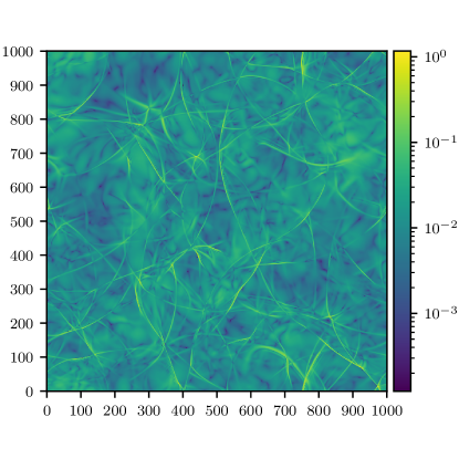
(b) $L\left|\mathbf{\omega}\right|$

Figure 13: The magnitude of the velocity (a) and the magnitude of the vorticity (b) in a slice of run XII during the period of strong shocks at $t=4.15t_{s}$. The vorticity has been plotted with a logarithmic color bar to make the different scales in the background vorticity more visible. The generated vorticity remains small, being largest at shock crests and in regions with overlapping shock waves. The maximum values for the quantities in the plots are 0.416 for the velocity, and 1.17 for $L\left|\mathbf{\omega}\right|$.

The behavior of the vorticity field is similar to that seen in the two-dimensional case, with the largest values obtained locally at shock fronts and in regions containing overlapping shock waves. The other contribution to the total vorticity comes from the background vorticity, which evolves slowly compared to the shock wave contribution. No formation of vortex like structures, like what was seen in 2D, can be seen in the vorticity components in the simulations. This could be due to the vortices being more difficult to visualize in three dimensions, but a more conclusive statement would require further study. Since this is not a focus of this paper, nor does it have an effect on any of the key results presented, we leave a more throughout study of the generated vorticity as potential future work.

IV The gravitational wave spectrum from decaying acoustic turbulence

The gravitational wave power spectrum resulting from linear non-decaying sound waves in the case of exact radiation domination is approximated by the sound shell model [25], which is based on the assumption that after the first order cosmological phase transition has come to an end, the fluid shells driven by the bubble walls continue to propagate as sound waves. The total velocity field after the phase transition can then be modelled as a superposition of the sound shells resulting from multiple bubbles, which can be treated as a Gaussian random field. The model also makes the assumption that the expansion of the universe can be neglected, which is a valid approximation for transitions which complete in much less than a Hubble time. This means that the model is only valid for transitions whose mean bubble separation $R_{\star}$ is much less than the Hubble length at the phase transition, giving the relation

$$r_{\star} \equiv R_{\star}H_{\star}$$

$$=\bar{v}_{0}t_{s}H_{\star}\ll 1\,.$$ (107)

The resulting GW power spectrum becomes a broken power law that at high wavenumbers goes as $k^{-3}$ and at low wavenumbers has a steep slope of $k^{9}$ when a static fluid energy spectrum with $E(k<k_{p})\propto k^{4}$ satisfying the causality conditions [49] is assumed.

In our previous work in Ref. [37] we estimated the gravitational wave power spectrum resulting from decaying acoustic turbulence by using its universal properties and a Gaussian approximation for the fluid velocity correlations. As the sound waves steepen into shocks, the Gaussianity of the velocity field is lost, but here we assume these deviations from Gaussianity to be small. We also neglect the expansion of the universe, which means that the timescale associated with non-linearities is much less than the Hubble time at the time of the phase transition ($t_{s}\ll H^{-1}_{\star}$), which is also taken to be the duration of the GW source (acoustic waves), so that one can use $t_{H_{\star}}\approx H^{-1}_{\star}$ as the cutoff time in the time integrals. We also employ the cosine type decoherence function for sound waves from the sound shell model. This way the expression for the GW power spectrum ends up being similar to that given by the sound shell model but with a time dependent energy spectrum that takes into account the model for the decay of the turbulence. We found that the GW power spectrum at wavenumbers higher than the peak is unchanged, but that there is a shallower intermediate power law that goes as $k^{11/2}$ between the peak and the steep $k^{9}$ power law, whose range depends on the energy-containing length scale of the fluid flow after a Hubble time.

However, the calculation in Ref. [25] (and as a result that in Ref. [37]) relies on the assumption that in the time dependent part of the expression for the GW power spectrum the time integrals can be approximated by taking the asymptotic limit $t\rightarrow\infty$, which makes the growth rate of the time dependent kernel function, denoted by $\Delta$, a sum of delta functions. This kind of asymptotic limit is not valid when GW production from a finite duration source is considered and contradicts the assumptions made about the GW source duration in relation to the Hubble time, on whose basis the expansion of the universe can be ignored. For the spectrum, it has the effect of extending the steep $k^{9}$ power law all the way to the origin of the $k$-axis, concealing the true low wavenumber behavior of the spectrum. Hence, recent studies in Refs. [33, 27] that consider finite time limits find that the steep $k^{9}$ spectrum is obtained only in a short range below the peak for high enough GW source durations, seen as a bump in the spectrum near the peak. In the expanding universe case the steep power law is even less prominent, appearing at much later times. At very low wavenumbers the spectrum goes as $k^{3}$, as causality requires [49], and for large enough source lifetimes a linearly increasing intermediate power law emerges between the two aforementioned power law ranges. Since these previously ignored contributions affect the shape of the spectrum considerably at small wavenumbers, the results found for the GW power spectrum in Ref. [37] should also be updated accordingly. In this section we discuss how the formulation of the GW power spectrum from decaying acoustic turbulence changes when the asymptotic limit is not taken in the time dependent kernel function $\Delta$ and how that changes the results found in the previous work.

The gravitational wave power spectrum resulting from the Gaussian approximation has been calculated in Ref. [33] both in the expanding and non-expanding universe cases. Here we adopt the result for ${t_{s}\ll H_{\star}^{-1}}$, meaning that we can ignore the expansion of the universe and approximate the duration of the GW source as $t_{H_{\star}}\approx H_{\star}^{-1}$, where $H_{\star}$ is the value of the Hubble parameter at the time of the phase transition. Since the fluid energy spectrum for decaying acoustic turbulence is time-dependent, our normalization differs from that of Eq. (2.12) in Ref. [33]. In the sound shell model the fluid shear stress unequal time correlator (UETC) takes the form [25].

$$U_{\Pi}(k,t_{1},t_{2})=\bar{w}_{e}\int\frac{d^{3}q}{(2\pi)^{3}}\frac{q^{2}}{\tilde{q}^{2}}(1-\mu^{2})^{2}G(q,t_{1},t_{2})G(\tilde{q},t_{1},t_{2})$$ (108)

where $\mathbf{\tilde{q}}=\mathbf{q}-\mathbf{k}$, $\mu=\mathbf{\hat{q}}\cdot\mathbf{\hat{k}}$, and $G$ is a function resulting from the velocity two-point functions. We now define a decoherence function $D(q,t_{1},t_{2})$ such that

$$G(q,t_{1},t_{2})=2\sqrt{P_{v}(q,t_{1})P_{v}(q,t_{2})}D(q,t_{1},t_{2})$$ (109)

where in the sound shell model

$$D(q,t_{1},t_{2})=\cos\left(c_{s}q(t_{1}-t_{2})\right)\,.$$ (110)

Under these assumptions, the gravitational wave power spectrum can be written as

$$\frac{1}{(H_{\star}L_{0})^{2}}\mathcal{P}_{\text{gw}}(k,t_{H_{\star}})=\mathcal{P}_{0}\int\limits_{0}^{\infty}dq\int\limits_{|q-k|}^{q+k}d\tilde{q}\,\rho(k,q,\tilde{q})\times\\ \int\limits_{0}^{t_{H_{\star}}}dt_{1}\int\limits_{0}^{t_{H_{\star}}}dt_{2}\,E(q,t_{1})E(\tilde{q},t_{2})\Delta(t_{1},t_{2},k,q,\tilde{q})\,,$$ (111)

where

$$\mathcal{P}_{0}=\frac{24(1+c_{s}^{2})^{2}}{L_{0}^{2}}$$ (112)

$$\rho(k,q,\tilde{q})=\frac{\left[4k^{2}q^{2}-(q^{2}+k^{2}-\tilde{q}^{2})^{2}\right]^{2}}{16q^{3}\tilde{q}^{3}k^{2}}\,,$$ (113)

and

$$\Delta(t_{1},t_{2},k,q,\tilde{q})=\frac{1}{2}\cos\left[k(t_{1}-t_{2})\right]\times\\ \cos\left[c_{s}q(t_{1}-t_{2})\right]\cos\left[c_{s}\tilde{q}(t_{1}-t_{2})\right]$$ (114)

is the integrand of the time-dependent kernel function in Ref. [25]. There the derivation proceeds by taking a time derivative of the equation corresponding to (111), and taking the asymptotic limit in time. The obtained final result for the asymptotic growth rate of the spectral density was then used in Ref. [37] to obtain the GW power spectrum. Here we now instead write the product of cosines as a sum of cosines

$$\Delta(t_{1},t_{2},k,q,\tilde{q})=\frac{1}{8}\sum_{\pm\pm}\cos\left[\omega_{\pm\pm}(t_{1}-t_{2})\right]$$ (115)

where

$$\omega_{\pm\pm}=k\pm c_{s}q\pm c_{s}\tilde{q}$$ (116)

and the sum runs over all four possible combination of signs in the above equation.

Next we need to define the fluid energy spectrum $E(k,t)$ for decaying acoustic turbulence. As seen in section III.3, we have

$$E(\kappa,t)=L(t)\mathcal{E}(t)\Psi(\kappa)\,,\quad\kappa=L(t)k\,,$$ (117)

where $\mathcal{E}(t)$ and $L(t)$ are given by equations (92) and (93) respectively. This form takes into account the reduction of the spectral amplitude resulting from the kinetic energy decay, and the shift in the energy containing length scale as the integral scale increases. Here we ignore the dissipation scale as the GW power from small scales is negligible, and assume a spectrum with a broken power law form, giving the spectral shape function $\Psi$ as

$$\Psi(\kappa)=\Psi_{0}\frac{(\kappa/\kappa_{p})^{\beta}}{1+(\kappa/\kappa_{p})^{\beta+2}}\,,$$ (118)

where we have written $\alpha=\beta+2$ so that the spectrum is assumed to obtain the $k^{-2}$ inertial range power law that is characteristic of classical acoustic turbulence. The parameters $\Psi_{0}$ and $\kappa_{p}$ are now determined by the value of $\beta$ only through equations (58) and (62), meaning they can be treated as constants in time. From equations (92) and (93) it follows that

$$\mathcal{E}(t)=\mathcal{E}_{0}\left(\frac{L(t)}{L_{0}}\right)^{-(\beta+1)}\,,$$ (119)

which can be used to replace the kinetic energy and write the equations only in terms of $L(t)$. This leads to some cancellation and the spectrum takes the form

$$E(k,t)=\Psi_{0}\mathcal{E}_{0}L_{0}\frac{\left[kL_{0}/\kappa_{p}\right]^{\beta}}{1+\left[kL(t)/\kappa_{p}\right]^{\beta+2}}\,.$$ (120)

The integrals over the wavenumber variables $q$ and $\tilde{q}$ can be made dimensionless with the change of variables $q=kx$, $\tilde{q}=ky$. Then by substituting the energy spectrum into equation (111) and by decomposing the cosines in Eq. (115) it is possible to write the GW power spectrum as

$$\frac{1}{(H_{\star}L_{0})^{2}}\mathcal{P}_{\text{gw}}(k,t_{H_{\star}})=\frac{\mathcal{P}_{0}}{128}\left(\frac{\Psi_{0}\mathcal{E}_{0}L_{0}^{\beta+1}}{\kappa_{p}^{\beta}}\right)^{2}k^{2(\beta+1)}\int\limits_{0}^{\infty}dx\int\limits_{|x-1|}^{x+1}dy\,\tilde{\rho}(x,y)\sum_{\pm\pm}\left[\int\limits_{0}^{t_{H_{\star}}}dt_{1}\frac{\cos(w_{\pm\pm}kt_{1})}{1+\left[xkL(t_{1})/\kappa_{p}\right]^{\beta+2}}\times\right.\\ \left.\int\limits_{0}^{t_{H_{\star}}}dt_{2}\frac{\cos(w_{\pm\pm}kt_{2})}{1+\left[ykL(t_{2})/\kappa_{p}\right]^{\beta+2}}+\int\limits_{0}^{t_{H_{\star}}}dt_{1}\frac{\sin(w_{\pm\pm}kt_{1})}{1+\left[xkL(t_{1})/\kappa_{p}\right]^{\beta+2}}\int\limits_{0}^{t_{H_{\star}}}dt_{2}\frac{\sin(w_{\pm\pm}kt_{2})}{1+\left[ykL(t_{2})/\kappa_{p}\right]^{\beta+2}}\right]$$ (121)

where

$$\tilde{\rho}(x,y)=(xy)^{\beta-3}\left[4x^{2}-\left(x^{2}+1-y^{2}\right)^{2}\right]^{2}$$ (122)

and we have rescaled

$$w_{\pm\pm}=1\pm c_{s}x\pm c_{s}y\,.$$ (123)

Using the time evolution equation for $L(t)$ in (93) allows us to write the time integrals as

$$\int\limits_{0}^{t_{H_{\star}}}dt_{1}\frac{\cos(w_{\pm\pm}kt_{1})}{1+\left[xkL(t_{1})/\kappa_{p}\right]^{\beta+2}}=\int\limits_{0}^{t_{H_{\star}}}dt_{1}\dfrac{\cos(w_{\pm\pm}kt_{1})}{1+\left(\frac{xkL_{0}}{\kappa_{p}}\right)^{\beta+2}\left(1+C\frac{t_{1}}{t_{s}}\right)^{\gamma}}\,,$$ (124)

where

$$\gamma\equiv\lambda(\beta+2)=\frac{2(\beta+2)}{\beta+3}\,.$$ (125)

The time integrals can be made dimensionless with a change of variables ${z=t/t_{s}}$. The gravitational wave power spectrum can then be written in terms of a time-dependent kernel function $\tilde{\Delta}$ as

$$\frac{1}{(H_{\star}L_{0})^{2}}\mathcal{P}_{\text{gw}}(kL_{0},t_{H_{\star}})=\widetilde{\mathcal{P}}_{0}\left(\frac{kL_{0}}{\kappa_{p}}\right)^{2(\beta+1)}\int\limits_{0}^{\infty}dx\int\limits_{|x-1|}^{x+1}dy\,\tilde{\rho}(x,y)\tilde{\Delta}(t_{H_{\star}},kL_{0},x,y)\,,$$ (126)

and using the previous relations for $\Psi_{0}$ and $\kappa_{p}$, and the definition of the shock formation time, the spectral amplitude obtains the form

$$\widetilde{\mathcal{P}}_{0}=\frac{3\left[(1+c_{s}^{2})(\beta+2)\right]^{2}}{16\pi^{2}}\bar{v}_{0}^{2}\sin^{2}\left[\frac{\pi(\beta+1)}{\beta+2}\right]\,,$$ (127)

and the kernel function can be written as

$$\tilde{\Delta}(t_{H_{\star}},kL_{0},x,y)=\sum_{\pm\pm}\left[\mathcal{I}_{c}(t_{H_{\star}},kL_{0},x,w_{\pm\pm}(x,y))\mathcal{I}_{c}(t_{H_{\star}},kL_{0},y,w_{\pm\pm}(x,y))\right.\\ \left.+\mathcal{I}_{s}(t_{H_{\star}},kL_{0},x,w_{\pm\pm}(x,y))\mathcal{I}_{s}(t_{H_{\star}},kL_{0},y,w_{\pm\pm}(x,y))\right]\,,$$ (128)

where we have defined the time integral functions $\mathcal{I}_{s}$ and $\mathcal{I}_{c}$ as

$$\mathcal{I}_{c}(t_{H_{\star}},kL_{0},\chi,w_{\pm\pm}(x,y)) =\int\limits_{0}^{z_{\star}}dz\dfrac{\cos\left(kL_{0}\frac{w_{\pm\pm}}{\bar{v}_{0}}z\right)}{1+\left(kL_{0}\frac{\chi}{\kappa_{p}}\right)^{\beta+2}\left(1+Cz\right)^{\gamma}}$$ (129)

$$\mathcal{I}_{s}(t_{H_{\star}},kL_{0},\chi,w_{\pm\pm}(x,y)) =\int\limits_{0}^{z_{\star}}dz\dfrac{\sin\left(kL_{0}\frac{w_{\pm\pm}}{\bar{v}_{0}}z\right)}{1+\left(kL_{0}\frac{\chi}{\kappa_{p}}\right)^{\beta+2}\left(1+Cz\right)^{\gamma}}\,,$$ (130)

with $z_{\star}=t_{H_{\star}}/t_{s}$. The gravitational wave power spectrum can now be solved from the above equations by setting values for the following four free parameters: The GW source lifetime in the units of shock formation times $z_{\star}=t_{H_{\star}}/t_{s}$, the decay constant $C$, The low-$k$ power law in the energy spectrum $\beta$, and the initial rms velocity of the flow $\bar{v}_{0}$. The stationary case is recovered with $C=0$.

We have studied the gravitational wave power spectrum by numerically integrating Eq. (126). We have chosen $\beta=4$ as predicted by causality, $C=0.2$ for the decay constant, which is close to the average effective value found in Table 3, and $\bar{v}_{0}=0.2$ for the rms velocity. We have also separated the GW spectrum into components as

$$\mathcal{P}_{\text{gw}}=\mathcal{P}_{++}+\mathcal{P}_{+-}+\mathcal{P}_{-+}+\mathcal{P}_{--}\,,$$ (131)

where each component contains one of the four terms in Eq. (128). Due to symmetry, we also have that $\mathcal{P}_{+-}=\mathcal{P}_{-+}$. The total gravitational wave spectrum, and the components have been plotted in Figure 14

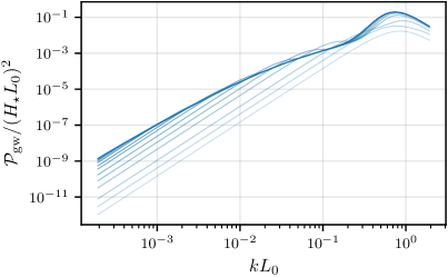
(a) Gravitational wave power spectrum.

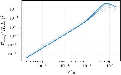
(b) Contribution from the $w_{--}$ terms.

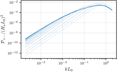
(c) Contribution from the $w_{+-}$ terms.

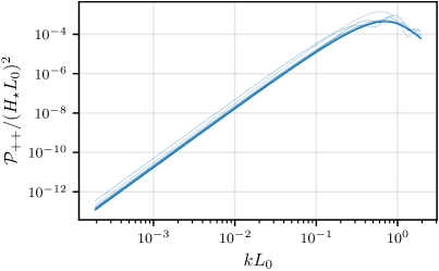
(d) Contribution from the $w_{++}$ terms.

Figure 14: The total gravitational wave power spectrum for decaying acoustic turbulence at various times obtained numerically from Equation (126), and the contributions from each of the four terms in the sum of Eq. (128). The times in question are approximately $t_{H_{\star}}/t_{s}\in[0.5,1,2,5,10,21,52,104,260,520,1039,1559,2078]$, with dark lines corresponding to late times. The chosen values for the free parameters are $\beta=4$, $\bar{v}_{0}=0.2$, and $C=0.2$. The spectrum converges to a constant value at late times.

for various GW source life times. As in the stationary case, where the energy spectrum of the fluid does not change over time, the large wavenumber behavior of the spectrum is set by the $\mathcal{P}_{--}$ component , whereas the shape at low wavenumbers follows from the $\mathcal{P}_{+-}$ component. The $\mathcal{P}_{++}$ component is subdominant at all wavenumbers. In the case of the asymptotic limit, it was found that a new $k^{5.5}$ power law appears below the peak whose range is set by the ratio of $L(t_{H_{\star}})/L_{0}$. Here the power law below the peak is also modified by the decay, as seen in Figure 15

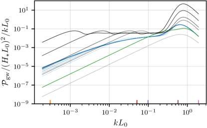
Figure 15: The converged spectra of Figure 14 colored in blue plotted together with the stationary spectra ($C=0$), colored in black, at times $t_{H_{\star}}/t_{s}\in[0.5,2,10,20,100,520]$. The stationary spectrum at $t_{H_{\star}}/t_{s}=2$ (green curve) coincides with the converged spectra of the decaying case at large wavenumbers.

that plots the late time decaying case spectra along with the stationary spectra (black lines) at various times. Instead of the steep $k^{9}$ power law behavior that is seen at late times in the stationary case, a shallower power law appears when the flow decays, while preserving the $k^{3}$ and $k^{-3}$ behaviors at the low and high wavenumber ends of the spectrum respectively. It can also be seen that the range of linear increase in $k$ at intermediate wavenumbers is no longer present in the decaying case, and scales close to linear only on a very short wavenumber range even at late times.

The change in the power law below the peak is caused by the increase of the integral length scale over time, which moves the peak of the fluid energy spectrum towards larger length scales. The power law gets shallower over time due to the change in the $\mathcal{P}_{--}$ component, as seen in Figure 14b, and the power law seen in the total spectrum is a superposition of the $\mathcal{P}_{--}$, $\mathcal{P}_{+-}$, and $\mathcal{P}_{-+}$ components. We have measured the power law by fitting in a range $kL_{0}\in[0.28,0.45]$ and the results for various GW source lifetimes can be seen in Table 4. The table also contains measurements for the power law in the $\mathcal{P}_{--}$ component with a fitting range of $kL_{0}\in[0.25,0.35]$.

$t_{H_{\star}}/t_{s}$	$L(t_{H_{\star}})/L_{0}$	$p$	$p_{-}$
21	$1.60$	$4.66\pm 0.08$	$6.49\pm 0.01$
52	$2.00$	$4.54\pm 0.05$	$6.40\pm 0.09$
104	$2.41$	$4.24\pm 0.05$	$5.83\pm 0.11$
260	$3.10$	$4.03\pm 0.03$	$5.22\pm 0.07$
520	$3.78$	$3.99\pm 0.03$	$5.06\pm 0.04$
1039	$4.60$	$3.98\pm 0.03$	$5.02\pm 0.03$
1559	$5.16$	$3.98\pm 0.02$	$5.01\pm 0.03$
2078	$5.60$	$3.98\pm 0.03$	$5.01\pm 0.03$

Table 4: The measured power law index $p$ in the power law range $k^{p}$ below the peak for the total GW power spectrum $\mathcal{P}_{\text{gw}}$ and the $\mathcal{P}_{--}$ component (denoted by $p_{-}$) for different GW source durations. The fitting range is $kL_{0}\in[0.28,0.45]$ for $\mathcal{P}_{\text{gw}}$, and $kL_{0}\in[0.25,0.35]$ for $\mathcal{P}_{--}$. The measurements indicate a convergence in the power law of the total spectrum towards $k^{4}$ at times for which $L(t_{H_{\star}})/L_{0}\gtrapprox 3.0$.

The measurements indicate that the power law in the $\mathcal{P}_{--}$ component converges towards $k^{5}$ at late times, and that the contributions from the other components ($\approx 2\mathcal{P}_{+-}$) result in a power law for the total spectrum that has converged to $k^{4}$ at times for which $L(t_{H_{\star}})/L_{0}\gtrapprox 3$.

The spectra of Figure 14 converge towards a constant value, due to the decay of the amplitude in the energy spectrum. In the stationary case convergence was seen at low wavenumbers, but the amplitude of the spectrum at the peak kept increasing linearly in time. Comparing Figures 14b and 14c shows that the convergence appears to be slower at small wavenumbers. Figure 16 shows the amplitude of the GW power spectrum at different wavenumbers as a function of time.

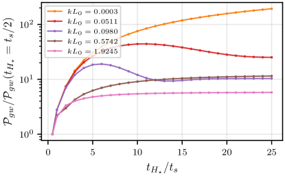
Figure 16: The magnitude of the decaying GW power spectrum at different wavenumbers as a function of the amount of shock formation times. The wavenumbers have been indicated in Figure 15 with colored ticks in the horizontal axis. The vertical axis has been normalized by the value of the spectrum at the first data point ($t_{H_{\star}}/t_{s}=1/2$). The spectrum has converged at $t_{H_{\star}}/t_{s}\geq 20$ to a reasonable degree in the vicinity of the peak.

The vertical axis has been normalized so that the curves coincide at $t_{H_{\star}}/t_{s}=1/2$. The figure shows the slower convergence with decreasing wavenumber, and indicates that the spectrum at wavenumbers around the peak has mostly converged at times $t_{H_{\star}}/t_{s}\geq 20$. The converged spectral amplitude at large wavenumbers past the peak coincides with the amplitude of the stationary case at $t_{H_{\star}}/t_{s}=2$, as can be seen from Figure 15, where the curve in question has been highlighted in green. This means that the effective lifetime of the decaying case with respect to the stationary case is about two times the timescale of the flow. However, the shape of the spectrum around the peak does not match the decaying case because the peak of the spectrum has not yet had enough time to develop for such early time in the decaying case. The stationary case is also recovered for flows that do not go through much change in a Hubble time, i.e. when the duration of the GW source is small compared to the flow timescale $t_{H_{\star}}\ll t_{s}$. Using Eq. (IV), this means $\bar{v}_{0}\ll r_{\star}$, so the stationary case is approximately valid in the limit of small initial rms velocities.

In conclusion, applying the sound shell model assumptions to the velocity field of decaying acoustic turbulence produces a converging GW power spectrum in the finite time limit, whose power law below the peak gets modified from the steep $k^{9}$ of the stationary case to a shallower one. For $\bar{v}_{0}=0.2$ it has converged to $k^{4}$ in the range $L(t_{H_{\star}})/L_{0}\gtrapprox 3.0$. The linearly increasing intermediate power law range is also greatly suppressed. We leave more careful study of the parameter space in terms of the rms velocity values $\bar{v}_{0}$, and the decay constant values $C$, along with generalizing the calculation for acoustic turbulence in the expanding universe case to a future work.

V Conclusions

We have studied decaying acoustic turbulence in three dimensions with the intention of verifying the universality of the results found in our previous two-dimensional study in Ref. [37], and updating the dimensionally dependent results to the 3D case. We have also improved the analysis by introducing previously missing terms to the fluid equations that affect the fluid around shock waves, and also by using a more accurate sixth order scheme when evaluating the spatial derivatives in the numerical simulations. The studied simulation runs have a wide range of initial Reynolds numbers and various different initial power laws in the energy spectra. A velocity limiter has been utilized to prevent the velocity from diverging around a single point and ruining the numerical solution in the few highest Reynolds number runs.

We have gone through the derivation of the fluid equations in detail for non-relativistic bulk velocities with the ultrarelativistic equation of state, and in addition to the $\nabla\ln\rho$ dependent terms that can obtain considerable contributions in the vicinity of shock waves and were missing in our previous work, we find an additional second order small term in the continuity equation that is missing in earlier literature [38]. We have studied the effect of these terms, and find that they smooth out the flows by reducing the maximum velocities present, and that they do not affect the power laws seen in the kinetic energy, integral length scale, or the energy spectrum after the shocks have formed.

The fluid equations are solved for a single shock travelling along one of the coordinate axes, and it is found that the new term in the continuity equation changes the shock shape compared to that found in our previous study [37]. However, the shock profile still maintains its hyperbolic tangent form, and direct comparison of the analytic solution with the numerical data obtained from an effectively one-dimensional shock tube run ends up being in an excellent agreement, as seen in Figure 7.

We have used the obtained shock profile to extract the time dependence of the decaying fluid energy spectrum and to write it in a self-similar form using the argument that the shape of the spectrum at small length scales depends on the shock shape, and changes over time as shocks dissipate. Since the computation depends on the dimensionality of the system, we find that it simplifies compared to the two-dimensional case, and find that the self-similar spectrum function can be written as a broken power law modulated by a function that depends on hyperbolic functions with arguments proportional to the inverse shock width. We have then used the self-similar spectral shape function as a fitting function to the numerical data for the energy spectrum from the simulations, and see a good match, especially in the low Reynolds number runs. We also extract the values for the fitting parameters, and find a good correspondence between the shock width parameter of the fitting function and the one in the shock width formula determined on dimensional grounds from the viscosity and rms velocity, and measure the proportionality constant.

The rate of change for the fluid kinetic energy can be derived from the fluid equations and is found to depend on three dominant contributions: the viscous dissipation, and two other $\nabla\cdot\mathbf{v}$ dependent terms that result from the pressure gradient term, and the non-linear terms. At late times the mean decay rate is set by the viscous dissipation term. The differential equation in this case can be solved using the previously found shape for the spectrum, and the universal properties of the $k^{-2}$ inertial range power law for classical acoustic turbulence, and the stationarity of the energy spectrum at low wavenumbers. This gives the kinetic energy as a function of time, that is found to decay following a power law form at late times.

We have used this result for the kinetic energy, and a broken power law form for the energy spectrum as fitting functions for simulation data with time averaging techniques to measure the numerical values of the power laws. The inertial range power law of the energy spectrum is measured to be $k^{-2.31\pm 0.02}$ by averaging over the tabulated values in runs with $40<\text{Re}<200$, thus obtaining slightly steeper values than what was found in the 2D case or expected for acoustic turbulence. The values also show approach towards the KP spectrum with increasing Reynolds number. However, higher Reynolds numbers runs are required to determine whether the values converge to $k^{-2}$ for the fluid equations employed here. The lowest Reynolds number runs have not been taken into account for these fits because there the shocks are relatively weak and the inertial range is short, which worsens the fits.

On the low-$k$ side the fits are not reliable for the high Reynolds number runs due to the peak wavenumber being close to the smallest wavenumber in the simulations, making the range too short. In the low Reynolds number runs the results for the power law are steeper than what was found in 2D, in accordance with the $k^{4}$ result predicted by causality conditions. The averaged power law index is found to be $k^{3.96\pm 0.12}$ when including only the measured values from runs with $\text{Re}<60$, that have standard deviations of about 0.5 or less. The energy spectrum obtains a universal form after the shocks have formed regardless of the initial power law values present in the spectrum.

Power law	All runs	Selected runs
$E(k)$: Inertial range	$-2.44\pm 0.02$	$-2.31\pm 0.02$
$E(k)$: Low wavenumber	$3.44\pm 0.21$	$3.96\pm 0.12$
Kinetic energy	$-1.30\pm 0.01$	$-1.33\pm 0.01$

Table 5: The averaged power law values for the inertial range power law $k^{\beta-\alpha}$ and the low wavenumber power law $k^{\beta}$ of the energy spectrum, and the kinetic energy decay power law $t^{-\zeta}$ obtained from the values of Tables 2 and 3. In the selected runs column, only runs with $\text{Re}>40$ have been taken into account for the inertial range, runs with $\text{Re}<60$ for the low-$k$ power law, and Run II has been excluded in the case of the kinetic energy decay power law for more optimal measurements.

For the kinetic energy, the measured decay power laws are found to be quite close to the values predicted by the low-$k$ power law index, and are steeper than the 2D results due to the change in the low-$k$ behavior. From the tabulated values it is found to go as $t^{-1.33\pm 0.01}$ at late times, when the greatly deviating value of Run II is ignored as an anomaly. The power law values for this and the previously discussed power laws with all runs included can be found in Table 5.

We have not included measurements of the integral length scale power law, nor the relations between the power laws, like we did in the 2D study. The peak being close to the lowest wavenumber causes oscillations in the peak, affecting the integral length scale value. There is also a decrease in its value after the shocks have formed that was not seen in 2D and makes the predicted time evolution function a bad fit, as it does not model a decreasing function. This effect could be caused by the lack of dynamic range in the simulations. We conclude that larger simulations are needed for better measurements of the low-$k$ power law of the energy spectrum, the integral length scale, and the previously mentioned relations, and to determine if the aforementioned change of shape in the integral length scale is affected by the size of the simulations. We also quickly touched on the generation of vorticity from irrotational initial conditions and found that there are more terms contributing than in the two-dimensional case, resulting both from the increase in dimensions, and from the additional terms in the fluid equations.

Lastly, we corrected an oversight that was found recently and affected our previous gravitational wave power spectrum calculation by ignoring sizeable contributions to the small wavenumber end of the spectrum. We lay out the corrected formulation for the GW power spectrum of decaying acoustic turbulence using the properties of the energy spectrum and the obtained model for the decay in the limit where the timescale of the flow is much shorter than the Hubble time at the time of the phase transition. The equations for the spectrum are then studied numerically, and we find that the shift in the peak of the fluid energy spectrum over time makes the power law below the peak shallower than the asymptotic $k^{9}$ found in the stationary case. For initial rms velocity value of 0.2, we find a convergence towards $k^{4}$ at times for which the integral length scale has grown to be at least about three times the initial value. The linearly scaling range is also noticeably suppressed compared to the stationary case. Due to the decay, there is convergence in the GW power spectrum whose amplitude at high wavenumbers corresponds to the amplitude of the stationary case at two shock formation times. The stationary case is recovered for flows whose timescale is large compared to the Hubble time at the time of the phase transition, which corresponds to the small initial rms velocity limit. We aim to provide a more detailed study of the paramater space in terms of the initial rms velocity $\bar{v}_{0}$ and the decay constant $C$, and their potential effects on the power law value and the convergence time in a future work.

Appendix A Effects of the velocity limiter

The velocity limiter detailed at the end of section III.1 has been used in the three highest Reynolds number runs labelled XIII-XV. These runs would end in a numerical blow up resulting from shock collisions during the strong shock phase if such a limiter was not employed. We argue that the use of a limiter of this kind is justified as long as it affects the fluid only locally at as few points as possible, and does not leave a lasting imprint on the fluid that changes the dynamics of the flow. In this section we shall take a closer look at how well these conditions are fulfilled, and how the limiter affects some of the quantities, especially those of interest to us in this work, by comparing the results of run XII, which is the highest Reynolds number run that can be finished without the limiter, to a run with the exact same initial condition and random phases, but where the limiter is activated after the shocks have formed. Thus, all deviations between these two runs are caused only by the velocity limiter. For this run, we have also used a threshold velocity of $v_{t}=0.4$, which is lower than the value of 0.5 we have used in the high Reynolds number runs in order to increase the amount of points that are affected by the limiter, thus making the effects more severe and noticeable.

When the limiter activates, the suppression truncates the solution to the wave equation, which generates an outward-moving wave at the activation point. Consecutive activations lead to a formation of a thumbprint-like pattern, which can be seen in the slice snapshots of the fluid, and whose magnitude depends on the suppression strength. These patterns are short-lived, vanishing in less than a single shock formation time in the velocity and the divergence. However, they leave a longer lasting imprint on the slowly evolving background vorticity, which is on the other hand very small in these initially non-vortical runs. The patterns can only be seen clearly in the highest Reynolds number run (XV), and any local deviations seen in the snapshots of the velocity limiter run XII are minimal at all times.

The amount of points affected by the velocity limiter depends on the threshold velocity, and on the rms velocity of the fluid. The amount of affected points at the largest (in total between all three of the velocity components) is about 200 for run XIII, about 3000 for run XIV, and about 4000 for run XV. For the velocity limiter version of run XII with the reduced threshold velocity, the amount of affected points ends up being about 2000 at the largest. In all cases, the largest amount of points affected are obtained after a few shock formations times when there are collisions between strong shocks. This means that even in our highest Reynolds number case, at most only 0.0004% of the total volume is affected by the limiter at any given time. Therefore, even with taking also into account the local and short-lived patterns that emerge from the activation points, the impact from the limiter on quantities derived through volume averages remains very small.

To test the effect of the limiter on averaged quantities, we have measured the magnitude of the largest deviations between the two runs for longitudinal and transverse components of the kinetic energy $\mathcal{E}$, the integral length scale $L$, and the enstrophy $\mathfrak{E}$ during the period of strong shocks, at six shock formation times. For the enstrophy

$$\mathfrak{E}=\left\langle\sum_{i,j=1}^{3}\left|\partial_{i}v_{j}\right|^{2}\right\rangle\,,$$ (132)

the longitudinal and transverse components can be written as

$$\mathfrak{E}_{\parallel}=\left\langle\left|\nabla\cdot\mathbf{v}\right|^{2}\right\rangle\,,\quad\mathfrak{E}_{\perp}=\left\langle\left|\nabla\times\mathbf{v}\right|^{2}\right\rangle\,.$$ (133)

It is worth noting that because the velocity limiter affects the maximum velocity in the flow, this changes the adaptive time step in Eq. (21). Therefore, the saving of the data takes place at slightly different times between the two runs, and the values obtained here result from comparing values that are closest in time. This means that there is a tiny time shift that introduces a small amount of additional uncertainty into the measurements. The deviations have been listed in Table 6 in terms of percentages.

Quantity	$\parallel$ (%)	$\perp$ (%)
$\mathcal{E}(t)$	$0.75$	$4.57$
$L(t)$	$0.43$	$3.00$
$\mathfrak{E}(t)$	$1.38$	$16.99$

Table 6: The largest amount of deviation caused by the velocity limiter with $v_{t}=0.4$ in run XII for the longitudinal and transverse kinetic energy, integral length scale, and enstrophy.

The largest deviations end up being less than $1\%$ for the longitudinal kinetic energy and integral length scale, and a bit over that for the longitudinal enstrophy. The deviation in the enstrophy being slightly higher is expected, as it depends on the divergence, which obtains its largest values at the shock waves and shock collisions, which is the domain of activation for the limiter. In the case transverse quantities, the deviations are larger. This is to be expected, as most of the vorticity is generated also at shocks and shock collisions. Even though the deviations end up being larger for the transverse quantities, the flows studied here are initially irrotational and are strongly dominated by longitudinal modes even at late times, meaning that the limiter does not have a noticeable effect on the total quantities. The deviations for the longitudinal quantities are also so small that there is no noticeable difference in the temporal behavior of the integral length scale and the kinetic energy or their power laws. The same also applies for the energy spectrum. Table 7 lists the measured power laws in the energy spectrum from Table 2, and the kinetic energy decay parameters from Table 3, along with the same measurements for the velocity limiter run.

Quantity	XII	XII VL
$\left\langle\alpha\right\rangle_{t}$	$3.924$	$3.900$
$\left\langle\beta\right\rangle_{t}$	$1.575$	$1.549$
$\left\langle\beta-\alpha\right\rangle_{t}$	$-2.349$	$-2.351$
$\left\langle\zeta\right\rangle_{t}$	$1.317$	$1.312$
$\left\langle C\right\rangle_{t}$	$0.200$	$0.201$

Table 7: Change in the measured power law values of Tables 2 and 3 resulting from using the velocity limiter with a threshold velocity of $v_{t}=0.4$ for run XII.

The deviations end up being small and well within the statistical fluctuations that result from random initial conditions, and the time averaging. When the time evolution of the longitudinal and transverse components of the enstrophy is considered, there ends up being some deviation from the values of the run with no limiter during the phase of strong shocks in both cases, but the values coincide again with the original run after about ten shock formation times. In the transverse components of some quantities, like $\mathcal{E}_{\perp}$, the limiter causes a shift in the values compared to the original run (reducing it in the case of the kinetic energy), which persists also after the limiter has stopped acting.

Figure 17 plots the maximum velocity of the flow for the original run XII (red line), and the one where the velocity limiter is active with a threshold velocity of ${v_{t}=0.4}$.

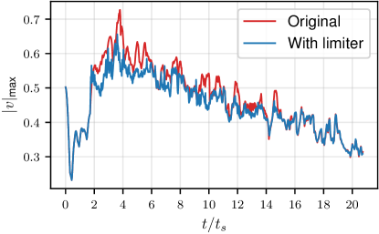
Figure 17: The maximum velocity measured in the fluid of run XII as a function of shock formation times (red line) and the same run with the velocity limiter active with a threshold velocity of $v_{t}=0.4$ (blue line). The limiter activates for the first time at $t\approx 1.71t_{s}$, and the last time at $t\approx 15.75t_{s}$. It can be seen that after the limiter is no longer active, the maximum velocity coincides with the original run, indicating that the limiter does not leave a lasting imprint on the shock waves.

The limiter activates for the first time around $t\approx 1.71t_{s}$, and for the last time around $t\approx 15.75$. The deviations in the maximum velocity are clearly seen while the limiter is active. After the flow has dissipated enough for the velocities to no longer exceed the threshold velocity, the maximum velocity coincides with the velocities of the original run, implying, that even though the limiter suppresses the highest velocities in the flow, it does not leave an imprint on them that persists to late times. All in all, we find that the velocity limiter does a good job at preventing a divergence in the velocity at shock collisions in high Reynolds numbers for the fluid equations employed here, while having very little effect for the dominant longitudinal components of quantities. The local effects in the velocity and energy density fields that emerge from the limiter are non-prominent and short-lived due to the suppression, and there are no significant changes in the temporal behavior of quantities or their power laws.

Appendix B Non-uniform kinematic viscosity for relativistic plasmas

When deriving the fluid equations in section II.1, we have (for simplicity and easier comparison with Ref. [37]) assumed the kinematic shear viscosity to be a constant, so that the relation between the kinematic and the dynamic viscosity is $\tilde{\eta}(\mathbf{x})=\eta\rho(\mathbf{x})$. However, for a relativistic plasma the dynamic shear viscosity depends on the temperature $T$ of the fluid along with the electromagnetic gauge coupling $e$ through the equation [50]

$$\tilde{\eta}\sim\frac{T^{3}}{e^{4}}\ln(1/e)\,.$$ (134)

The temperature can be related to the energy density using the early universe Friedmann equation

$$8\pi G\rho=\frac{\pi^{2}}{30}g_{*}(T)\frac{T^{4}}{m_{\text{p}}^{2}}\,,$$ (135)

where $m_{\text{p}}$ is the Planck mass, $G$ the universal gravitational constant, and $g_{*}(T)$ the effective number of relativistic degrees of freedom. The function $g_{*}(T)$ changes slowly during the radiation dominated era, so it can be approximated as a constant, which gives the temperature as

$$T=\left(\frac{240\pi G_{N}M_{\text{pl}}^{2}}{\pi^{2}g_{*}}\right)^{1/4}\rho^{1/4}\equiv C_{T}\rho^{1/4}\,.$$ (136)

This means that

$$\tilde{\eta}(\mathbf{x})\sim C_{T}^{3}\frac{\ln(1/e)}{e^{4}}\rho(\mathbf{x})^{3/4}\,,$$ (137)

so that instead of being linear in $\rho$, the shear viscosity is proportional to $\rho^{3/4}$. Its gradient then becomes

$$\nabla\tilde{\eta}(\mathbf{x})\sim C^{3}\frac{\ln(1/e)}{e^{4}}\cdot\frac{3}{4}\rho(\mathbf{x})^{-1/4}\nabla\rho(\mathbf{x})$$ (138)

$$\Rightarrow \nabla\tilde{\eta}(\mathbf{x})=\frac{3}{4}\tilde{\eta}(\mathbf{x})\nabla\ln\rho(\mathbf{x})\,.$$ (139)

During the derivation of the viscosity dependent part of the fluid equations, the additional term that contains the shear rate tensor picks up an additional factor because of the above equation. The RHS of Equation 20 can then be written as

$$\frac{\eta}{1+c_{s}^{2}}\left[\nabla^{2}\mathbf{v}+\frac{1}{3}\nabla(\nabla\cdot\mathbf{v})+\frac{3}{2}\mathbf{S}\cdot\nabla\ln\rho\right]\,,$$ (140)

where the kinematic shear viscosity $\eta$ is now non-uniform, because using Eq. (137) we can write it as

$$\eta(\mathbf{x})=\frac{\tilde{\eta}(\mathbf{x})}{\rho(\mathbf{x})}\equiv\eta_{0}\left(\frac{\rho(\mathbf{x})}{\rho_{0}}\right)^{-1/4}\,.$$ (141)

Due to the power of the energy density being small, this does not lead to large deviations from the constant viscosity value of $\eta_{0}$. However, this does mean that the viscosity at the location of the shock waves is slightly reduced due to the energy density being large there. This leads to a small increase in the numerical oscillations at the crests of the shocks, and thus reduces the range of obtainable Reynolds numbers in the simulations (without resorting to e.g. velocity limiters). For example, the velocity in Run XII would diverge with this kind of viscosity enabled.

To test the effects of the non-uniform viscosity of Eq. (141), we have reproduced runs V and XI with it, using a value of $\eta_{0}=0.04$. Much like in Appendix A when studying the effects of the velocity limiter, the deviations in the case of both runs are found to be small, with the transverse quantities being affected a bit more due to the decreased viscosity at the shock waves and its effects on the vorticity generation. This also causes a small change in the high wavenumber end of the energy spectrum in the form of a stronger bottleneck effect, which makes the bump at the fold between the inertial and dissipation ranges very slightly higher. This is seen in the case of Run XI in Figure 18.

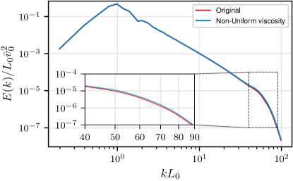
Figure 18: The energy spectrum for Runs XI (red curve) and XI NUV (blue curve), the latter of which is the same run but with the non-uniform viscosity of Eqs. (140) and (141) enabled. The reduction in the viscosity at the shock waves leads to a slightly increased bottleneck effect at the high wavenumber end of the spectrum.

Regardless, the shape of the spectrum after the bump, which is affected by the shock shape, is not noticeably changed, indicating that the modifications resulting from the non-uniform viscosity to the calculation in section III.2 are small, and that the results found there are still be approximately valid. The change in the power laws of Tables 2 and 3 resulting from the non-uniform viscosity are listed in Table 8. Also listed is the change in the $\kappa_{s}$ parameter of Table 1, which relates to the shock width parameter.

Quantity	V	V NUV	XI	XI NUV
$\left\langle\alpha\right\rangle_{t}$	$6.875$	$6.866$	$5.521$	$5.517$
$\left\langle\beta\right\rangle_{t}$	$4.270$	$4.269$	$3.184$	$3.183$
$\left\langle\beta-\alpha\right\rangle_{t}$	$-2.605$	$-2.597$	$-2.338$	$-2.334$
$\left\langle\zeta\right\rangle_{t}$	$1.447$	$1.449$	$1.283$	$1.283$
$\left\langle C\right\rangle_{t}$	$0.177$	$0.176$	$0.201$	$0.200$
$\kappa_{s}$	$7.37$	$7.43$	$19.50$	$19.75$

Table 8: Change in the power law values of Tables 2 and 3, and the $\kappa_{s}$ parameter of Table 1, resulting from using the non-uniform viscosity (NUV) for runs V and XI.

The differences are small, and within the statistical fluctuations resulting from random initial conditions and the time averaging. Hence, we conclude that for the runs used in this work, the use of the simpler viscosity in Eq. (20) still produces approximately the same results as would be obtained by using the non-uniform viscosity of Eq. (141) for relativistic plasmas.

Appendix C Simulation code and initial conditions

The data used in this work has been obtained with a Python-based simulation code. Due to its interpreted nature, Python is slow, and is, by itself, ill-suited for high performance computing. In order to obtain adequate performance, the most computationally demanding parts of the code need to be optimized. In fact, with proper optimization methods, a Python-based simulation code can obtain near C-like performance.

Cython [51] has been used to optimize routines that contain nested loops over array values, such as spatial derivatives and the distribution of random phases in Fourier space to obtain random initial conditions. Element-wise array computations have been accelerated with NumExpr [52]. The code supports parallelization, so that computational tasks can be distributed to multiple processor cores. The arrays are slab distributed in the $x$-direction using the MPI for Python [53] and the mpi4py-fft [54] packages so that the advancement of the fluid, and the handling and saving of data on each slab are performed by a single processor core. Other key packages include NumPy [55] for multidimensional arrays, and SciPy [56] for computational tools, such as curve fitting using $\mathtt{scipy.optimize.curve\_fit}$, and numerical integration with $\mathtt{scipy.integrate.quad}$. The routines have been used in obtaining values for the fitting parameters in the results section, and the gravitational wave power spectra in section IV. Because the integrands present in $\mathcal{I}_{c}$ and $\mathcal{I}_{s}$ of equations (129) and (130) are highly oscillatory at high wavenumbers and late times, sine and cosine weights have been used in the $\mathtt{quad}$ routine to obtain accurate results in these cases.

Evaluation of quantities containing integrals over the Fourier space, like the rms velocities through Eq. (29) or the integral length scale in Eq. (30) has been carried out by writing the integrals in terms of the reciprocal lattice volume element and moving to the discretized limit, where the radial integrals become sums over the arrays via

$$\int d^{3}k\rightarrow\frac{(2\pi)^{3}}{V}\sum\limits_{\bar{k}}\,,$$ (142)

where the volume $V=N^{3}(\Delta x)(\Delta y)(\Delta z)$. The initial conditions are given in terms of the longitudinal and transverse spectral densities

$$P_{\parallel}(|\mathbf{k}|) =\frac{1}{V}\Big{(}|v_{x}^{\parallel}(\mathbf{k})|^{2}+|v_{y}^{\parallel}(\mathbf{k})|^{2}+|v_{z}^{\parallel}(\mathbf{k})|^{2}\Big{)}$$ (143)

$$P_{\perp}(|\mathbf{k}|) =\frac{1}{V}\Big{(}|v_{x}^{\perp}(\mathbf{k})|^{2}+|v_{y}^{\perp}(\mathbf{k})|^{2}+|v_{z}^{\perp}(\mathbf{k})|^{2}\Big{)}\,,$$ (144)

where $P_{\parallel}$ and $P_{\perp}$ are given in the form of Eq. (26). The longitudinal and transverse velocity components can be related to their Cartesian components by the projection operators

$$v_{i}^{\parallel}(\mathbf{k})=\hat{k}_{i}\hat{k}_{k}v_{j}(\mathbf{k})$$ (145)

$$v_{i}^{\perp}(\mathbf{k})=(\delta_{ij}-\hat{k}_{i}\hat{k}_{j})v_{j}(\mathbf{k})\,,$$ (146)

where the hats denote unit vectors. The transverse component consists of two vectors perpendicular to the unit vector $\hat{k}$, so that the total velocity in the Fourier space can be written as

$$v(\mathbf{k})=v^{\parallel}\hat{\mathbf{k}}+v_{t_{1}}\hat{e}_{1}(\mathbf{k})+v_{t_{2}}\hat{e}_{2}(\mathbf{k})\,,$$ (147)

where the unit vectors $\hat{e}_{1}$ and $\hat{e}_{2}$ form an orthogonal basis as

$$\hat{e}_{1}(\mathbf{k})=\hat{\mathbf{q}}\times\hat{\mathbf{k}}\,,\quad\hat{e}_{1}(\mathbf{k})=\hat{\mathbf{k}}\times\hat{e}_{1}(\mathbf{k})\,.$$ (148)

The vector $\hat{\mathbf{q}}$ sets the direction of the components and has been chosen so that there is no anisotropy in the rms values of the velocity field between the Cartesian components in real space. The way the power in $P_{\perp}$ is distributed to the velocity components $v_{t_{1}}$ and $v_{t_{2}}$ can be chosen freely, which makes it possible to generate e.g. helical velocity fields (albeit in this work all runs are initialized to have zero vorticity initially). The Fourier space components in Eq. (148) are given random phases $\varphi$ in the range $[-\pi,\pi[$ in such a way that

$$v_{i}(\mathbf{k})=v_{i}(\mathbf{k})e^{i\varphi}\,,$$ (149)

and so that $v_{i}(-\mathbf{k})=v_{i}^{\star}(\mathbf{k})$, giving a real space velocity array that is real. A random field generated from three components will have longitudinal and transverse rms velocities in the proportion 1:2, so the real space velocity components are then obtained by proper scaling and inverse Fourier transforms. The Fourier transform routine used is the $D$-dimensional parallel Fast Fourier Transform routine provided by the mpi4py-fft package. The radial energy spectra or spectral densities, like in Figure 6, are obtained from Eqs. (143) and (144) by radially averaging the values in the array over spherical shells of width $\Delta k$, which is the reciprocal lattice spacing. The averaging is performed up to the wavenumber corresponding to the Nyquist frequency, meaning that the corner regions of the cubic arrays are not taken into account.

The runs featured in this paper have a resolution of $1000^{3}$ and their initial conditions are listed in Table 9 in the order of increasing initial Reynolds number. The Runs have been conducted on CSC’s (Finnish IT center for science) supercomputer Puhti. They are labeled with Roman numerals in the first column, and columns 2-4 and 6-7 contain the initial values for the parameters that appear in the longitudinal spectral density found in Eq. (26). The fifth column shows the inertial range power law value in the longitudinal energy spectrum $E_{\parallel}(k)$, where the corresponding low-$k$ power law is obtained as $\beta=\xi+2$. The $k_{p}$ values are given in the units of the reciprocal lattice spacing $\Delta k=2\pi/1000\approx 0.0063$, and the amplitude of the spectral density has been scaled by the inverse of the volume to reduce the magnitude of the tabulated values. The amplitudes have also been rounded to three significant figures. The precise values used for these are found in the run files that are referred to at the end of this section. The final three columns list the shock formation time of the run, the initial rms velocity, and the initial Reynolds number respectively. These have been measured from the initial fluid state in the simulations. For all runs $P_{\perp}=0$, meaning that each run has zero vorticity initially. All spectra also have the exponential suppression wavenumber at $k_{d}=(100\sqrt{5}/\pi)\Delta k$, and the kinematic shear viscosity constant for all runs is $\eta=0.04$. The initial energy density is uniform with $\rho(\mathbf{x})=\rho_{0}=1.0$.

The Python simulation code can be found in Ref. [57], and the spectrum and time series data along with the run files and visualization for each of the featured runs is found in Ref. [58].

ID	$\alpha$	$\xi$	$\delta$	$\beta-\alpha$	$k_{p}$	$A/V$	$t_{s}$	$\bar{v}$	Re
I	$12$	$3$	$4$	$-7$	$32.0\Delta k$	$497$	$60$	$0.094$	$10.0$
II	$6$	$2$	$3$	$-2$	$8.5\Delta k$	$3290$	$100$	$0.103$	$19.9$
III	$12$	$2$	$4$	$-8$	$19.0\Delta k$	$2360$	$100$	$0.107$	$21.3$
IV	$9$	$3$	$3$	$-4$	$10.0\Delta k$	$8840$	$100$	$0.132$	$32.6$
V	$20$	$4$	$5$	$-14$	$15.0\Delta k$	$17900$	$100$	$0.134$	$33.6$
VI	$10$	$4$	$2$	$-4$	$8.5\Delta k$	$12000$	$100$	$0.154$	$44.2$
VII	$15$	$8$	$3$	$-5$	$7.2\Delta k$	$51100$	$100$	$0.173$	$56.2$
VIII	$26$	$5$	$13$	$-19$	$10.0\Delta k$	$5430000$	$203$	$0.129$	$63.8$
IX	$11$	$1$	$11/2$	$-8$	$9.0\Delta k$	$70400$	$201$	$0.142$	$75.6$
X	$20$	$3$	$5$	$-15$	$7.3\Delta k$	$148000$	$201$	$0.148$	$82.5$
XI	$16$	$2$	$4$	$-12$	$7.0\Delta k$	$93800$	$204$	$0.154$	$90.7$
XII	$21$	$0$	$3$	$-19$	$7.9\Delta k$	$23100$	$193$	$0.173$	$108.6$
XIII	$32$	$1$	$8$	$-29$	$7.5\Delta k$	$231000$	$207$	$0.204$	$161.5$
XIV	$33$	$0$	$11$	$-31$	$10.5\Delta k$	$99300$	$192$	$0.222$	$178.2$
XV	$52$	$2$	$13$	$-48$	$7.0\Delta k$	$1200000$	$206$	$0.223$	$191.7$

Table 9: The parameter values at the initial time for the $1000^{3}$-resolution runs featured in this paper. The $k_{p}$ values are given in terms of the reciprocal lattice spacing $\Delta k=2\pi/1000\approx 0.0063$. The parameter $\beta=\xi+2$ is the low-$k$ power law in the energy spectrum of the fluid. The spectral indices in columns 2-4, and the spectral amplitude in column 7 correspond to those in Eq. (26). Also listed are the initial shock timescale, rms velocity, and Reynolds number, measured from the initial velocity field.

References

- Caprini et al. [2020] C. Caprini et al., Detecting gravitational waves from cosmological phase transitions with LISA: an update, JCAP 03, 024, arXiv:1910.13125 [astro-ph.CO] .
- Guth and Weinberg [1981] A. H. Guth and E. J. Weinberg, Cosmological Consequences of a First Order Phase Transition in the SU(5) Grand Unified Model, Phys. Rev. D23, 876 (1981).
- Steinhardt [1982] P. J. Steinhardt, Relativistic detonation waves and bubble growth in false vacuum decay, Phys.Rev. D25, 2074 (1982).
- Ignatius et al. [1994] J. Ignatius, K. Kajantie, H. Kurki-Suonio, and M. Laine, The growth of bubbles in cosmological phase transitions, Phys. Rev. D 49, 3854 (1994), arXiv:astro-ph/9309059 .
- Espinosa et al. [2010] J. R. Espinosa, T. Konstandin, J. M. No, and G. Servant, Energy Budget of Cosmological First-order Phase Transitions, JCAP 06, 028, arXiv:1004.4187 [hep-ph] .
- Witten [1984] E. Witten, Cosmic Separation of Phases, Phys.Rev. D30, 272 (1984).
- Hogan [1986] C. J. Hogan, Gravitational radiation from cosmological phase transitions, Mon. Not. Roy. Astron. Soc. 218, 629 (1986).
- Kosowsky et al. [2002] A. Kosowsky, A. Mack, and T. Kahniashvili, Gravitational radiation from cosmological turbulence, Phys. Rev. D 66, 024030 (2002), arXiv:astro-ph/0111483 .
- Christensen [2019] N. Christensen, Stochastic Gravitational Wave Backgrounds, Rept. Prog. Phys. 82, 016903 (2019), arXiv:1811.08797 [gr-qc] .
- Caprini and Figueroa [2018] C. Caprini and D. G. Figueroa, Cosmological Backgrounds of Gravitational Waves, Class. Quant. Grav. 35, 163001 (2018), arXiv:1801.04268 [astro-ph.CO] .
- Amaro-Seoane et al. [2017] P. Amaro-Seoane et al. (LISA), Laser Interferometer Space Antenna, (2017), arXiv:1702.00786 [astro-ph.IM] .
- Ellis et al. [2019] J. Ellis, M. Lewicki, and J. M. No, On the Maximal Strength of a First-Order Electroweak Phase Transition and its Gravitational Wave Signal, JCAP 04, 003, arXiv:1809.08242 [hep-ph] .
- Ellis et al. [2020] J. Ellis, M. Lewicki, and J. M. No, Gravitational waves from first-order cosmological phase transitions: lifetime of the sound wave source, JCAP 07, 050, arXiv:2003.07360 [hep-ph] .
- Cutting et al. [2020] D. Cutting, M. Hindmarsh, and D. J. Weir, Vorticity, kinetic energy, and suppressed gravitational wave production in strong first order phase transitions, Phys. Rev. Lett. 125, 021302 (2020), arXiv:1906.00480 [hep-ph] .
- Cutting et al. [2022] D. Cutting, E. Vilhonen, and D. J. Weir, Droplet collapse during strongly supercooled transitions, Phys. Rev. D 106, 103524 (2022), arXiv:2204.03396 [astro-ph.CO] .
- Brandenburg et al. [2017] A. Brandenburg, T. Kahniashvili, S. Mandal, A. Roper Pol, A. G. Tevzadze, and T. Vachaspati, Evolution of hydromagnetic turbulence from the electroweak phase transition, Phys. Rev. D 96, 123528 (2017), arXiv:1711.03804 [astro-ph.CO] .
- Niksa et al. [2018] P. Niksa, M. Schlederer, and G. Sigl, Gravitational Waves produced by Compressible MHD Turbulence from Cosmological Phase Transitions, Class. Quant. Grav. 35, 144001 (2018), arXiv:1803.02271 [astro-ph.CO] .
- Roper Pol et al. [2020] A. Roper Pol, S. Mandal, A. Brandenburg, T. Kahniashvili, and A. Kosowsky, Numerical simulations of gravitational waves from early-universe turbulence, Phys. Rev. D 102, 083512 (2020), arXiv:1903.08585 [astro-ph.CO] .
- Auclair et al. [2022] P. Auclair, C. Caprini, D. Cutting, M. Hindmarsh, K. Rummukainen, D. A. Steer, and D. J. Weir, Generation of gravitational waves from freely decaying turbulence, JCAP 09, 029, arXiv:2205.02588 [astro-ph.CO] .
- Landau and Lifshitz [1987] L. Landau and E. Lifshitz, Fluid Mechanics (Pergamon Press, 2nd edition, 1987).
- Pen and Turok [2016] U.-L. Pen and N. Turok, Shocks in the Early Universe, Phys. Rev. Lett. 117, 131301 (2016), arXiv:1510.02985 [astro-ph.CO] .
- L’vov et al. [1997] V. S. L’vov, Y. L’vov, A. C. Newell, and V. Zakharov, Statistical description of acoustic turbulence, Physical Review E 56, 390 (1997).
- L’vov et al. [2000] V. S. L’vov, Y. V. L’vov, and A. Pomyalov, Anisotropic spectra of acoustic turbulence, Phys. Rev. E 61, 2586 (2000), arXiv:chao-dyn/9905032 .
- Hindmarsh [2018] M. Hindmarsh, Sound shell model for acoustic gravitational wave production at a first-order phase transition in the early Universe, Phys. Rev. Lett. 120, 071301 (2018), arXiv:1608.04735 [astro-ph.CO] .
- Hindmarsh and Hijazi [2019] M. Hindmarsh and M. Hijazi, Gravitational waves from first order cosmological phase transitions in the Sound Shell Model, JCAP 12, 062, arXiv:1909.10040 [astro-ph.CO] .
- Guo et al. [2021] H.-K. Guo, K. Sinha, D. Vagie, and G. White, Phase Transitions in an Expanding Universe: Stochastic Gravitational Waves in Standard and Non-Standard Histories, JCAP 01, 001, arXiv:2007.08537 [hep-ph] .
- Roper Pol et al. [2023] A. Roper Pol, S. Procacci, and C. Caprini, Characterization of the gravitational wave spectrum from sound waves within the sound shell model, (2023), arXiv:2308.12943 [gr-qc] .
- Hindmarsh et al. [2014] M. Hindmarsh, S. J. Huber, K. Rummukainen, and D. J. Weir, Gravitational waves from the sound of a first order phase transition, Phys. Rev. Lett. 112, 041301 (2014), arXiv:1304.2433 [hep-ph] .
- Hindmarsh et al. [2015] M. Hindmarsh, S. J. Huber, K. Rummukainen, and D. J. Weir, Numerical simulations of acoustically generated gravitational waves at a first order phase transition, Phys. Rev. D 92, 123009 (2015), arXiv:1504.03291 [astro-ph.CO] .
- Hindmarsh et al. [2017] M. Hindmarsh, S. J. Huber, K. Rummukainen, and D. J. Weir, Shape of the acoustic gravitational wave power spectrum from a first order phase transition, Phys. Rev. D 96, 103520 (2017), [Erratum: Phys.Rev.D 101, 089902(E) (2020)], arXiv:1704.05871 [astro-ph.CO] .
- Konstandin [2018] T. Konstandin, Gravitational radiation from a bulk flow model, JCAP 03, 047, arXiv:1712.06869 [astro-ph.CO] .
- Jinno et al. [2023] R. Jinno, T. Konstandin, H. Rubira, and I. Stomberg, Higgsless simulations of cosmological phase transitions and gravitational waves, JCAP 02, 011, arXiv:2209.04369 [astro-ph.CO] .
- Sharma et al. [2023] R. Sharma, J. Dahl, A. Brandenburg, and M. Hindmarsh, Shallow relic gravitational wave spectrum with acoustic peak, JCAP 12, 042, arXiv:2308.12916 [gr-qc] .
- Caprini et al. [2009] C. Caprini, R. Durrer, and G. Servant, The stochastic gravitational wave background from turbulence and magnetic fields generated by a first-order phase transition, JCAP 12, 024, arXiv:0909.0622 [astro-ph.CO] .
- Jinno et al. [2021] R. Jinno, T. Konstandin, and H. Rubira, A hybrid simulation of gravitational wave production in first-order phase transitions, JCAP 04, 014, arXiv:2010.00971 [astro-ph.CO] .
- Brandenburg et al. [2021] A. Brandenburg, G. Gogoberidze, T. Kahniashvili, S. Mandal, A. Roper Pol, and N. Shenoy, The scalar, vector, and tensor modes in gravitational wave turbulence simulations, Class. Quant. Grav. 38, 145002 (2021), arXiv:2103.01140 [gr-qc] .
- Dahl et al. [2022] J. Dahl, M. Hindmarsh, K. Rummukainen, and D. J. Weir, Decay of acoustic turbulence in two dimensions and implications for cosmological gravitational waves, Physical Review D 106, 10.1103/physrevd.106.063511 (2022).
- Brandenburg et al. [1996] A. Brandenburg, K. Enqvist, and P. Olesen, Large scale magnetic fields from hydromagnetic turbulence in the very early universe, Phys. Rev. D 54, 1291 (1996), arXiv:astro-ph/9602031 .
- Rezzolla and Zanotti [2014] L. L. Rezzolla and O. Zanotti, Relativistic hydrodynamics (Oxford University Press, Oxford, 2014).
- Arnold et al. [2006a] P. B. Arnold, C. Dogan, and G. D. Moore, The Bulk Viscosity of High-Temperature QCD, Phys. Rev. D 74, 085021 (2006a), arXiv:hep-ph/0608012 .
- Fornberg [1988] B. Fornberg, Generation of finite difference formulas on arbitrarily spaced grids, Mathematics of Computation 51, 699 (1988).
- Brandenburg [2001] A. Brandenburg, Computational aspects of astrophysical mhd and turbulence, (2001), arXiv:astro-ph/0109497 .
- pc_[2023] Pencil Code manual (2023).
- Burgers [1948] J. Burgers, A mathematical model illustrating the theory of turbulence, Advances in Applied Mechanics 1, 171 (1948).
- Kadomtsev and Petviashvilil [1973] B. Kadomtsev and V. Petviashvilil, Dokl. Akad. Nauk SSSR 208, 794 (1973).
- Falkovich [1994] G. Falkovich, Bottleneck phenomenon in developed turbulence, Physics of Fluids 6, 1411 (1994).
- Dobler et al. [2003] W. Dobler, N. E. L. Haugen, T. A. Yousef, and A. Brandenburg, Bottleneck effect in three-dimensional turbulence simulations, Physical Review E 68, 10.1103/physreve.68.026304 (2003).
- Saffman [1971] P. G. Saffman, On the spectrum and decay of random two-dimensional vorticity distributions at large reynolds number, Studies in Applied Mathematics 50, 10.1002/sapm1971504377 (1971).
- Durrer and Caprini [2003] R. Durrer and C. Caprini, Primordial magnetic fields and causality, JCAP 11, 010, arXiv:astro-ph/0305059 .
- Arnold et al. [2006b] P. B. Arnold, C. Dogan, and G. D. Moore, The Bulk Viscosity of High-Temperature QCD, Phys. Rev. D 74, 085021 (2006b), arXiv:hep-ph/0608012 .
- Behnel et al. [2011] S. Behnel, R. Bradshaw, C. Citro, L. Dalcin, D. S. Seljebotn, and K. Smith, Cython: The best of both worlds, Computing in Science Engineering 13, 31 (2011).
- Cooke et al. [2018] D. Cooke, T. Hochberg, F. Alted, I. Vilata, M. Wiebe, G. de Menten, A. Valentino, and R. A. McLeod, NumExpr: Fast numerical expression evaluator for NumPy (2018).
- Dalcín et al. [2005] L. Dalcín, R. Paz, and M. Storti, Mpi for python, Journal of Parallel and Distributed Computing 65, 1108 (2005).
- Dalcin, Lisandro and Mortensen, Mikael and Keyes, David E [2019] Dalcin, Lisandro and Mortensen, Mikael and Keyes, David E, Fast parallel multidimensional FFT using advanced MPI, Journal of Parallel and Distributed Computing 10.1016/j.jpdc.2019.02.006 (2019).
- Harris et al. [2020] C. R. Harris et al., Array programming with NumPy, Nature 585, 357 (2020).
- Virtanen et al. [2020] P. Virtanen et al., SciPy 1.0: Fundamental Algorithms for Scientific Computing in Python, Nature Methods 17, 261 (2020).
- Dahl [2024a] J. Dahl, Simulation code for fluids in three dimensions (2024a), https://doi.org/10.5281/zenodo.10580342.
- Dahl [2024b] J. Dahl, Dataset and visualization of numerical simulations of decaying acoustic turbulence in three dimensions, 10.5281/zenodo.10580913 (2024b), https://doi.org/10.5281/zenodo.10580913.