Relic gravitational waves from the chiral magnetic effect

Abstract

Relic gravitational waves (GWs) can be produced by primordial magnetic fields. However, not much is known about the resulting GW amplitudes and their dependence on the details of the generation mechanism. Here we treat magnetic field generation through the chiral magnetic effect (CME) as a generic mechanism and explore its dependence on the speed of generation (the product of magnetic diffusivity and characteristic wavenumber) and the speed characterizing the maximum magnetic field strength expected from the CME. When the latter exceeds the former (regime I), the regime applicable to the early universe, we obtain an inverse cascade with moderate GW energy that scales with the third power of the magnetic energy. When the generation speed exceeds the CME limit (regime II), the GW energy continues to increase without a corresponding increase of magnetic energy. In the early kinematic phase, the GW energy spectrum (per linear wavenumber interval) has opposite slopes in both regimes and is characterized by an inertial range spectrum in regime I and a white noise spectrum in regime II. The occurrence of these two slopes is shown to be a generic consequence of a nearly monochromatic exponential growth of the magnetic field. The resulting GW energy is found to be proportional to the fifth power of the limiting CME speed and the first power of the generation speed.

1. Introduction

The chiral magnetic effect (CME) describes an electric current along a magnetic field carried by electrically charged chiral fermions (Vilenkin, 1980). This effect has been discussed as one of several possible mechanisms for significantly amplifying primordial magnetic fields in the early universe (Boyarsky et al., 2012, 2015). It works as a dynamo effect that destabilizes the state of vanishing magnetic field and causes an arbitrarily weak seed field to grow exponentially for a limited time (Joyce & Shaposhnikov, 1997). Excitation sets in when the fermion chiral asymmetry is large enough. However, owing to the existence of a conservation law for the sum of magnetic helicity and chiral asymmetry, the CME becomes continuously depleted until nearly all the initial chiral asymmetry is turned into magnetic helicity (Boyarsky et al., 2012, 2015). Thus, the initial chiral asymmetry determines the final value of the product of the mean squared magnetic field $B_{\rm rms}^{2}$ and the magnetic correlation length $\xi_{\rm M}$, forming a proxy for magnetic helicity in case of a fully helical field. For realistic parameters describing our universe, $B_{\rm rms}^{2}\xi_{\rm M}$ is expected to be of the order of or below $(10^{-18}\,{\rm G})^{2}\,{\rm Mpc}$ (Brandenburg et al., 2017b). This value is below the lower limit of $B_{\rm rms}^{2}\xi_{\rm M}>(10^{-16}\,{\rm G})^{2}\,{\rm Mpc}$ that is inferred from the non-observations of GeV-energy halos around TeV blazars (Aharonian et al., 2006; Neronov & Vovk, 2010; Taylor et al., 2011). Yet the question can be raised, whether the resulting magnetic stress could still be large enough to produce measurable gravitational waves (GWs).

Another severe problem are the very small length scales associated with the CME. An upper bound for the wavenumber associated with the chiral asymmetry in comoving units is $k_{*}\equiv k_{\rm B}T/\hbar c=12\,{\rm cm}^{-1}$, where $k_{\rm B}$ is the Boltzmann constant, $\hbar$ is the reduced Planck constant, $c$ is the speed of light, and $T=2.7\,{\rm K}$ is the present day temperature. Assuming a field strength of $1\,\mu{\rm G}$, the value of $k_{*}$ is compatible with the upper bound on the magnetic helicity of $(10^{-18}\,{\rm G})^{2}\,{\rm Mpc}$ (Brandenburg et al., 2017b). This value of $k_{*}$ corresponds to very small length scales, because the CME is a microphysical effect involving just $\hbar$, $c$, and $k_{\rm B}$ as relevant natural constants, but not Newton’s constant or the Planck mass; see also Brandenburg et al. (2017a). The Hubble radius, by contrast, does involve Newton’s constant and is much bigger ($1.8\times 10^{15}\,{\rm cm}$). In units of the inverse Hubble radius, the characteristic scale of the CME corresponds to a wavenumber of about $2\times 10^{16}$; see Equation (1) of Kahniashvili et al. (2013), and is associated with a very high GW frequency of $4\times 10^{11}\,{\rm Hz}$; see Equation (51) of Kosowsky et al. (2002). On the other hand, at the time of the electroweak phase transition, the Hubble scale corresponds to a frequency in the mHz range, which is the range accessible to the Laser Interferometer Space Antenna. Larger length scales have been argued to be possible by invoking strongly out-of-equilibrium magnetic field generation during preheating (Díaz-Gil, 2008a, b), or during inflation (Sharma et al., 2020; Okano & Fujita, 2021). In addition, the actual GW frequency could be several orders of magnitude smaller owing to the inverse cascade associated with the CME. By the time the magnetic field has reached its maximum, its typical length scale can therefore be significantly larger than the scale at which the field was originally produced. After that time, the magnetic length scales continue to increase as the magnetic energy decreases. However, Roper Pol et al. (2020b) found that the resulting GW energy is determined just by the maximum field strength. It is therefore unclear whether the late phase of magnetic decay is still relevant to GW production.

Although the CME may not open a viable pathway for explaining the primordial magnetic field, it has the advantage of providing a self-consistent mechanism for explaining not just a certain field strength and length scale, but also a certain time dependence of its generation, independent of any extra assumptions. Thus, it may serve as a proxy for other generation mechanisms. It is then interesting to investigate GWs produced by the CME as a mechanism that is likely to contain qualitatively valid aspects of primordial magnetic field generation; see the recent work by Anand et al. (2019) for analytic approaches addressing GW production from the CME at energies much above the electroweak scale, or the approaches of Sharma et al. (2020) and Okano & Fujita (2021) addressing GW production from helical magnetogenesis during inflation. These works give more optimistic prospects about the resulting magnetic field generation than Brandenburg et al. (2017b). Therefore, in the present study our aim is to understand the detailed relationship between the strengths of magnetic field and GWs, as well as their typical time and length scales.

In the past, theoretical GW energy spectra have been calculated mostly using analytical approaches; see Deryagin et al. (1987) for an early pioneering investigation and Caprini et al. (2019) for a recent review. Numerical approaches have recently been applied to GWs, driven by acoustic turbulence from first order phase transitions (Hindmarsh et al., 2015). A general uncertainty in simulating relic GWs from primordial turbulent sources is due to our ignorance about suitable initial conditions or generation mechanisms. When a turbulent state is invoked as initial condition, the GW amplitude is determined almost entirely by the fact that then the GW source, i.e., the turbulent stress, jumps instantaneously from zero to a finite value (Roper Pol et al., 2020a). By contrast, when driving turbulence gradually by applying some forcing in the magnetohydrodynamic (MHD) equations, the resulting GW amplitude depends on the details of how the turbulence develops and later declines; see Kahniashvili et al. (2021) for a more systematic investigation. These problems motivate our present study of GWs from the CME, too.

A number of interesting aspects of turbulence from the CME are already known. In particular, depending on the relative rates of magnetic field generation, on the one hand, and depletion of the CME, on the other, different regimes of turbulence can be distinguished (Brandenburg et al., 2017b). If the depletion is low, the maximum magnetic field strength is high and a turbulent spectrum with an inertial range emerges before the turbulence starts to decay in a self-similar fashion. If the depletion is high, on the other hand, no turbulent inertial range develops. How the resulting GW amplitude depends on the governing parameters of the CME-driven field generation is unclear and illuminating this is the main purpose of this paper. Although the process is physically motivated, we choose parameters that are motivated by our attempt to understand the relationship between magnetic field generation and the resulting GWs in any conceivable regime. Our parameters are therefore not those relevant to the early universe, nor are they necessarily physically realizable. Nevertheless, the present work may prove to be important for guiding our intuition about GW production from primordial turbulent sources.

2. The model

2.1. Basic equations

The MHD equations for an ultrarelativistic quark-gluon plasma in a flat expanding universe in the radiation-dominated era after the electroweak phase transition can be written in terms of conformal time and comoving coordinates such that the expansion no longer appears explicitly (Brandenburg et al., 1996, 2017a; Durrer & Neronov, 2013), except for the GW equation; see below. The bulk motions are assumed to be subrelativistic.

We quantify the chiral asymmetry through the imbalance between the number densities $n_{\rm L}$ and $n_{\rm R}$ of left- and right-handed fermions, respectively, as

$${\mu}_{5}=24\,\alpha_{\rm em}\,(n_{\rm L}-n_{\rm R})\,(\hbar c/k_{\rm B}T)^{2},$$ (1)

employing the normalization used by Rogachevskii et al. (2017). Here, $\alpha_{\rm em}$ is the fine structure constant. The index 5 is commonly chosen in this context and reminiscent of the fifth Dirac matrix $\gamma_{5}$, central in defining particle chirality. We should point out that our ${\mu}_{5}$ has the unit of inverse length and is related to the chiral chemical potential (with units of energy) through an extra $\hbar c/4\alpha_{\rm em}$ factor; see Schober et al. (2020).

We follow here the normalization of Roper Pol et al. (2020a, b), where the Heaviside-Lorentz system of units is used for the magnetic field and the scale factor $a(t)$ is set to unity at the time $t_{*}$ of the electroweak phase transition (denoted by an asterisk). The Hubble parameter $H$ at $t_{*}$ is $H_{*}=t_{*}^{-1}$. All quantities are made nondimensional by normalizing time by $t_{*}$, velocities by the speed of light $c$, and the density $\rho$ by the critical density $\rho_{\rm crit}$ for a flat universe. Spatial coordinates are then normalized by the Hubble scale $c/H_{*}$. Consequently, ${\mu}_{5}$ is normalized by $H_{*}/c$. To obtain the comoving magnetic field in gauss, one has to multiply it by $\sqrt{4\pi\rho_{\rm crit}}c$.

The governing equations for the magnetic field $\bm{B}$ and ${\mu}_{5}$ can then be written as (Rogachevskii et al., 2017; Schober et al., 2018)

$${\partial\bm{B}\over\partial t} = \mbox{\boldmath$\nabla$}{}\times[\bm{u}\times\bm{B}+\eta({\mu}_{5}\bm{B}-\mbox{\boldmath$J$}{})],\;\;\;\mbox{\boldmath$J$}{}=\mbox{\boldmath$\nabla$}{}\times\bm{B},\;$$ (2)

$${{\rm D}{}{\mu}_{5}\over{\rm D}{}t} = -\lambda\,\eta\left({\mu}_{5}\bm{B}-\mbox{\boldmath$J$}{}\right)\cdot\bm{B}+D_{5}\nabla^{2}{\mu}_{5}-\Gamma_{\rm\!f}{\mu}_{5},$$ (3)

where ${\rm D}{}/{\rm D}{}t\equiv\partial/\partial t+\bm{u}\cdot\mbox{\boldmath$\nabla$}{}$ is the advective derivative, $\eta$ is the magnetic diffusivity, $\lambda$ characterizes the depletion of ${\mu}_{5}$ as the magnetic field increases, $D_{5}$ is a chiral diffusion coefficient, and $\Gamma_{\rm\!f}$ is the flipping rate (see Boyarsky et al., 2021, for a recent calculation). These equations have been derived under the assumption $\eta\to 0$; see Rogachevskii et al. (2017) for details. Brandenburg et al. (2017b) found that for $k_{\rm B}T=100\,{\rm GeV}$ and if $\mu_{50}$ is produced thermally, relevant to the time of the electroweak phase transition, $\Gamma_{\rm\!f}/\eta{\mu}_{5}^{2}\approx 10^{-7}$, that is, the time $1/\Gamma_{\rm\!f}$ is much longer than the e-folding time of the fastest growing magnetic mode; see Section 2.2. Hence, we put $\Gamma_{\rm\!f}=0$ from now on. The plasma velocity $\bm{u}$ and the density $\rho$ (which includes the rest mass density) obey the momentum and energy equations

$${{\rm D}{}\bm{u}\over{\rm D}{}t} = {2\over\rho}\mbox{\boldmath$\nabla$}{}\cdot\left(\rho\nu\mbox{\boldmath${\sf S}$}{}\right)-{1\over 4}\mbox{\boldmath$\nabla$}{}\ln\rho+{\bm{u}\over 3}\left(\mbox{\boldmath$\nabla$}{}\cdot\bm{u}+\bm{u}\cdot\mbox{\boldmath$\nabla$}{}\ln\rho\right)$$ (4)

$$- {\bm{u}\over\rho}\left[\bm{u}\cdot(\mbox{\boldmath$J$}{}\times\bm{B})+\eta\mbox{\boldmath$J$}{}^{2}\right]+{3\over 4\rho}\mbox{\boldmath$J$}{}\times\bm{B},$$

$${\partial\ln\rho\over\partial t} = -\frac{4}{3}\left(\mbox{\boldmath$\nabla$}{}\cdot\bm{u}+\bm{u}\cdot\mbox{\boldmath$\nabla$}{}\ln\rho\right)+{1\over\rho}\left[\bm{u}\cdot(\mbox{\boldmath$J$}{}\times\bm{B})+\eta\mbox{\boldmath$J$}{}^{2}\right]\!,$$

where ${\sf S}_{ij}=(u_{i,j}+u_{j,i})/2-\delta_{ij}\mbox{\boldmath$\nabla$}{}\cdot\bm{u}/3$ are the components of the rate-of-strain tensor with commas denoting partial derivatives, $\nu$ is the kinematic viscosity, and the ultrarelativistic equation of state $p=\rho/3$ has been employed. In the following, we assume uniform $\nu$, $\eta$, and $D_{5}$ and vary them such that $\nu=\eta=D_{5}$.

The GW equation in the radiation era for the scaled strain tensor ${\sf h}$ with ${\sf h}_{ij}=a{\sf h}_{ij}^{\rm phys}$ is written in Fourier space as (Roper Pol et al., 2020a, b)

$$\frac{\partial^{2}}{\partial t^{2}}\tilde{h}_{+/\times}(\bm{k},t)+k^{2}\tilde{h}_{+/\times}(\bm{k},t)={6\over t}\tilde{T}_{+/\times}(\bm{k},t),$$ (5)

where $\tilde{h}_{+/\times}={\sf e}_{ij}^{+/\times}({\sf P}_{il}{\sf P}_{jm}-{\textstyle{1\over 2}}{\sf P}_{ij}{\sf P}_{lm})\,\tilde{{\sf h}}_{lm}(\bm{k},t)$ are the Fourier-transformed $+$ and $\times$ modes of ${\sf h}$, with ${\sf e}^{+}_{ij}(\bm{k})\,\,=\,e_{i}^{1}e_{j}^{1}-e_{i}^{2}e_{j}^{2}$ and ${\sf e}^{\times}_{ij}(\bm{k})\,=\,e_{i}^{1}e_{j}^{2}+e_{i}^{2}e_{j}^{1}$ being the linear polarization basis, $\mbox{\boldmath$e$}{}^{1}$ and $\mbox{\boldmath$e$}{}^{2}$ are unit vectors perpendicular to $\bm{k}$ and perpendicular to each other, and ${\sf P}_{ij}(\bm{k})=\delta_{ij}-k_{i}k_{j}$ is the projection operator. $\tilde{T}_{+/\times}$ are defined analogously and normalized by the critical density. The stress is composed of magnetic and kinetic contributions, ${\sf T}_{ij}=\frac{4}{3}\gamma_{\rm Lor}^{2}\rho u_{i}u_{j}-B_{i}B_{j}+...$, where $\gamma_{\rm Lor}=(1-\bm{u}^{2})^{-1/2}$ is the Lorentz factor, and the ellipsis denotes terms proportional to $\delta_{ij}$, not contributing to $\tilde{T}_{+/\times}$. Since we use the nonrelativistic equations, we put $\gamma_{\rm Lor}=1$, except for one case shown in Appendix A, where $\gamma_{\rm Lor}\neq 1$. Our equations apply to the time after the electroweak phase transition $t_{\ast}$, so our normalized time obeys $t\geq 1$. Furthermore, to compute the relic observable GW energy at the present time, we have to multiply ${\cal E}_{\rm GW}^{\rm sat}$ by the square of the ratio of the Hubble parameters and the fourth power of the ratio of scale factors between the moment of the electroweak phase transition and today, which is $1.64\times 10^{-5}$; see Roper Pol et al. (2020a, b) for details.

As already alluded to above, the system of equations (2), (3) describing the CME must be regarded as partly phenomenological and subject to extensions and modifications. A purely helical magnetic field with wavenumber $k={\mu}_{5}={\rm const}{}$, for example, can never decay if $\Gamma_{\rm\!f}=0$, and yet it would lead to Ohmic heating. However, those effects are not critical to the dynamics that we are concerned with in this paper and will therefore be ignored. Likewise, an extra $-{\mu}_{5}\mbox{\boldmath$\nabla$}{}\cdot\bm{u}$ term on the right-hand side of Equation (3) is necessary for a proper conservation equation. However, this would not make a noticeable difference because $\mbox{\boldmath$\nabla$}{}\cdot\bm{u}$ is always small; see Appendix A for a demonstration. It should also be noted that, in comparison with earlier work, this is the first time that the CME has been solved together with Equations (4), which contain additional 4/3 factors. We refer to Appendix A of Brandenburg et al. (2017a) for the differences to standard MHD.

2.2. Basic phenomenology of the chiral magnetic effect

The CME introduces two important characteristic quantities into the system: $\lambda$ and the initial value of ${\mu}_{5}$, ${\mu}_{50}={\mu}_{5}(t=1)$, both assumed uniform. Different evolutionary scenarios can be envisaged depending on their values. Following Brandenburg et al. (2017b), we use the fact that $\lambda^{-1}$ has the dimension of energy per unit length and ${\mu}_{50}$ has the dimension of inverse length, and identify two characteristic velocities:

$$v_{\lambda}={\mu}_{50}/\lambda^{1/2},\quad\quad v_{\mu}={\mu}_{50}\eta.$$ (6)

We recall that we have used here dimensionless quantities. We can identify two regimes of interest:

$$\eta k_{1}<v_{\mu}<v_{\lambda}\quad\mbox{(regime I)},$$ (7)

$$\eta k_{1}<v_{\lambda}<v_{\mu}\quad\mbox{(regime II)},$$ (8)

where $k_{1}$ is the smallest wavenumber in the domain and $\eta k_{1}<v_{\mu}$ is necessary for magnetic field excitation. The case $v_{\lambda}<\eta k_{1}$ is highly diffusive and was not considered. In regime I, if the ratio $v_{\lambda}/v_{\mu}=\left[\eta\,\lambda^{1/2}\right]^{-1}$ is large, the $\lambda$ term is unimportant and ${\mu}_{5}$ will only change slowly as the magnetic field grows. Once the magnetic field exceeds a critical value of around $v_{\mu}$, it becomes turbulent; see Brandenburg et al. (2017b). In that paper, both $v_{\mu}$ and $v_{\lambda}$ were assumed to be less than the speed of sound, but this is not a physically imposed constraint and will be relaxed in the present work. Brandenburg et al. (2017b) also found that the crossover between the regimes occurs when $v_{\lambda}/v_{\mu}\approx 8$. Regarding the resulting GW production, however, we shall find evidence for a crossover at $v_{\lambda}/v_{\mu}\approx 1$. One should also remember that $v_{\mu}$ and $v_{\lambda}$ do not correspond to physically realizable speeds and are therefore not constrained to be below unity. Let us mention at this point that, using the calculation of Arnold et al. (2000) for the value of $\eta$ and the expression $\lambda=3\hbar c\,(8\alpha_{\rm em}/k_{\rm B}T)^{2}$ from Rogachevskii et al. (2017), Brandenburg et al. (2017b) estimated that $v_{\mu}\approx 2\times 10^{-5}$ and $v_{\lambda}\approx 0.05$ for ${\mu}_{50}=2\times 10^{16}$.

If ${\mu}_{50}\neq 0$, the CME determines primarily the magnetic helicity that can subsequently be generated. This is a direct consequence of the conservation law for the (weighted) sum of mean magnetic helicity density and mean ${\mu}_{5}$, i.e., the total mean chirality (Rogachevskii et al., 2017),

$${\textstyle{1\over 2}}\lambda\,\langle\mbox{\boldmath$A$}{}\cdot\bm{B}\rangle+\langle{\mu}_{5}\rangle={\rm const}{},$$ (9)

where $A$ with $\bm{B}=\mbox{\boldmath$\nabla$}{}\times\mbox{\boldmath$A$}{}$ is the magnetic vector potential, and the brackets denote averaging over a closed or periodic volume; see Appendix A for a discussion of the accuracy of Equation (9). If the initial magnetic helicity is arbitrarily small, the constant in Equation (9) can be set to ${\mu}_{50}$. Neglecting the influence of the turbulent flow $\bm{u}$ and inhomogeneities of ${\mu}_{5}$, the generated magnetic field is fully helical (Beltrami), and its helicity can be characterized by its wavenumber $k_{\rm M}$ and the mean magnetic energy density $\langle\bm{B}^{2}\rangle/2$ through $\langle\mbox{\boldmath$A$}{}\cdot\bm{B}\rangle\approx\langle\bm{B}^{2}\rangle/k_{\rm M}$. Therefore, once all the initial ${\mu}_{5}$ is used up, we have

$$\langle\bm{B}^{2}\rangle/k_{\rm M}\approx 2{\mu}_{50}/\lambda.$$ (10)

Interestingly, the value of $\eta$ does not enter this estimate. It does, however, determine the initial growth rate $\gamma(k)$ of the magnetic field, which adopts its maximum, $\gamma_{0}\equiv\eta{\mu}_{50}^{2}/4$, at the wavenumber $k_{\mu}\equiv{\mu}_{50}/2$. Using $k_{\rm M}\approx k_{\mu}$, we expect

$$\langle\bm{B}^{2}\rangle\lesssim{\mu}_{50}^{2}/\lambda\equiv v_{\lambda}^{2},$$ (11)

so large magnetic fields are expected for large values of ${\mu}_{50}$ and small values of $\lambda$. The fact that $v_{\lambda}$ characterizes the maximum magnetic field strength justifies the name “limiting CME speed”. On the other hand, as one can express $v_{\mu}$ by the maximum growth rate and the corresponding wavenumber as $2\gamma_{0}/k_{\mu}$, we may call it “generation speed” in analogy to “phase speed” for a wave.

2.3. Magnetic energy spectrum from the CME

To estimate the amount of magnetic energy production from the CME, we adopt the semi-empirical model of Brandenburg et al. (2017b), who proposed to construct the magnetic energy spectrum such that it had the $k^{-2}$ slope that is characteristic of magnetically dominated turbulence, with energy injection predominantly at the wavenumber $k_{\mu}$. For an intermediate time interval around the magnetic energy maximum, they then proposed the following form for the magnetic energy spectrum $E_{\rm M}(k)$ (with normalization $\int E_{\rm M}(k)dk=\langle\bm{B}^{2}\rangle/2\equiv{\cal E}_{\rm M}$) as a function of wavenumber $k$ and the parameters $\eta$, ${\mu}_{50}$, and $\lambda$ that govern the CME:

$$E_{\rm M}(k)=C_{5}\,{\mu}_{50}^{3}\eta^{2}k^{-2}\quad\mbox{($k_{\lambda}\leq k\leq k_{\mu}$)}$$ (12)

where $C_{5}\approx 16$ is a Kolmogorov-type constant,

$$k_{\lambda}=\sqrt{\lambda C_{5}/C_{\lambda}}\,{\mu}_{50}\eta\approx 4{\mu}_{50}\eta\lambda^{1/2}$$ (13)

is the wavenumber corresponding to the outer scale of the $k^{-2}$ subrange, and $C_{\lambda}\approx 1$ is another empirical constant (Brandenburg et al., 2017b). Of course, Equation (12) can only hold if $k_{\lambda}\leq k_{\mu}$. In regime I, $k_{\lambda}$ is the typical wavenumber of the magnetic field when it has reached maximum strength.

A detailed sketch illustrating the different spectral subranges is Figure 1 of Brandenburg et al. (2017b), who also confirmed the form of Equation (12) through simulations. The present simulations also support the existence of the different subranges.

2.4. GW energy scaling

The work of Roper Pol et al. (2020b) has shown that the GW energy is not just proportional to the square of the magnetic energy, but also proportional to the square of the dominating length scale (or inverse wavenumber) of $\bm{B}$. For example, their Runs ini2 and ini3 have the same magnetic energy, but in ini3, the spectral peak was at a ten times smaller wavenumber, corresponding to just ten turbulent eddies per Hubble horizon. The resulting GW energy was then about a hundred times larger. To leading order, the GW energy, normalized by the critical energy of the universe, is given by ${\cal E}_{\rm GW}=\langle\dot{h}_{+}^{2}+\dot{h}_{\times}^{2}\rangle/6$; see Roper Pol et al. (2020a) for details regarding the 1/6 factor and additional correction terms. Roper Pol et al. (2020b) studied different types of turbulence and confirmed the quadratic relationship between the maximum magnetic energy, ${\cal E}_{\rm M}^{\max}$ and the saturation value of the GW energy, ${\cal E}_{\rm GW}^{\rm sat}$ in the form

$${\cal E}_{\rm GW}^{\rm sat}\approx(q{\cal E}_{\rm M}^{\max}/k_{\rm peak})^{2},$$ (14)

where $k_{\rm peak}$ is the wavenumber of the peak of the spectrum ($k_{\rm peak}=600$ in most of their cases, and $60$ in the case where a hundred times larger ${\cal E}_{\rm GW}^{\rm sat}$ was found, suggesting an inverse quadratic relationship), and $q$ is an empirical efficiency parameter that is about $0.9$ for their cases with a turbulent initial MHD state (but no forcing), $1.8$ in their simulations with forced MHD turbulence, and $11$ in their simulations of forced acoustic turbulence, where ${\cal E}_{\rm M}^{\max}$ has to be replaced by the maximum kinetic energy. Larger values of $q$ correspond to more efficient conversion of magnetic or kinetic energy into GW energy. The reason why acoustic turbulence is more efficient is unclear, but may be speculated to lie in its more vigorous time dependence.

2.5. Numerical aspects

We solve Equations (2)–(5) using the Pencil Code (Pencil Code Collaboration, 2021), which is a finite difference code that is third order in time and sixth order in space, except that Equation (5) is solved exactly between subsequent time instants; see Roper Pol et al. (2020a) for details. For most of our simulations, we use $512^{3}$ meshpoints, which turned out to be sufficient for the present investigations. The lowest wavenumber in our computational domain, $k_{1}$, is chosen to be $100$ for many of our runs. The side length of the cubical computational domain is then $2\pi/k_{1}$, which is chosen to be large enough so that the governing dynamics is well captured by the simulations, but small enough to resolve the smallest length scales. In many cases, we verified that the results are independent of the choice of $k_{1}$.

Throughout his work, we present spectra of various quantities. We denote this operation as $\mbox{\rm Sp}(\cdot)$, which is performed as integration over concentric shells in wavenumber space. For a scalar quantity $f$ it reads $\mbox{\rm Sp}(f(\bm{x}))=k^{2}\int|\tilde{f}(\bm{k})|^{2}d\Omega_{k}$, where $\Omega_{k}$ is the solid angle in $\bm{k}$ space, while for the tensor ${\sf h}$ we put $\mbox{\rm Sp}(\mbox{\boldmath${\sf h}$}{})=\mbox{\rm Sp}(h_{+})+\mbox{\rm Sp}(h_{\times})$, and likewise for $\dot{\mbox{\boldmath${\sf h}$}{}}$ and ${\sf T}$. Thus, the GW energy spectrum is given by $E_{\rm GW}(k)\equiv\mbox{\rm Sp}(\dot{\mbox{\boldmath${\sf h}$}{}})/6$ and the magnetic one by $E_{\rm M}(k)\equiv[\mbox{\rm Sp}(B_{x})+\mbox{\rm Sp}(B_{y})+\mbox{\rm Sp}(B_{z})]/2$.

3. Results

We have performed a range of simulations where we vary $\eta$, $\lambda$, and ${\mu}_{50}$, studying the influence of these parameters in turn.

3.1. Comparison with earlier GW energy scaling

To put our new simulations into context, it is convenient to compare our values of ${\cal E}_{\rm GW}^{\rm sat}$ for given ${\cal E}_{\rm M}^{\max}$ with those obtained by Roper Pol et al. (2020b). We show in Figure 1 a plot similar to their Figure 7, depicting our simulations with ${\mu}_{50}=10^{4}$, grouped into four series with $\lambda^{1/2}$ in the range from $5\times 10^{4}$ to $5\times 10^{3}$. In each of those series, we vary $\eta$. The resulting values of ${\cal E}_{\rm M}^{\max}$ and ${\cal E}_{\rm GW}^{\rm sat}$ are summarized in Table LABEL:Tsummary, along with the four input parameters $\eta$, $\lambda^{1/2}$, ${\mu}_{50}$, and $k_{1}$, as well as several derived quantities: $\eta k_{1}$, $v_{\mu}$, $v_{\lambda}$, $\eta{\mu}_{50}^{2}$, and $k_{\lambda}$ (provided $k_{\lambda}\leq{\mu}_{50}/2$). In the last column, we also give according to Equation (14)

$$q=k_{\rm peak}\sqrt{{\cal E}_{\rm GW}^{\rm sat}}/{\cal E}_{\rm M}^{\max},$$ (15)

where we estimate $k_{\rm peak}=k_{\mu}\min(1,v_{\mu}/v_{\lambda})$. This means that $k_{\rm peak}=k_{\mu}$ when $v_{\mu}>v_{\lambda}$ (regime II) and $k_{\rm peak}=k_{\lambda}/4$ when $v_{\mu}<v_{\lambda}$ (regime I); see also Equation (13).

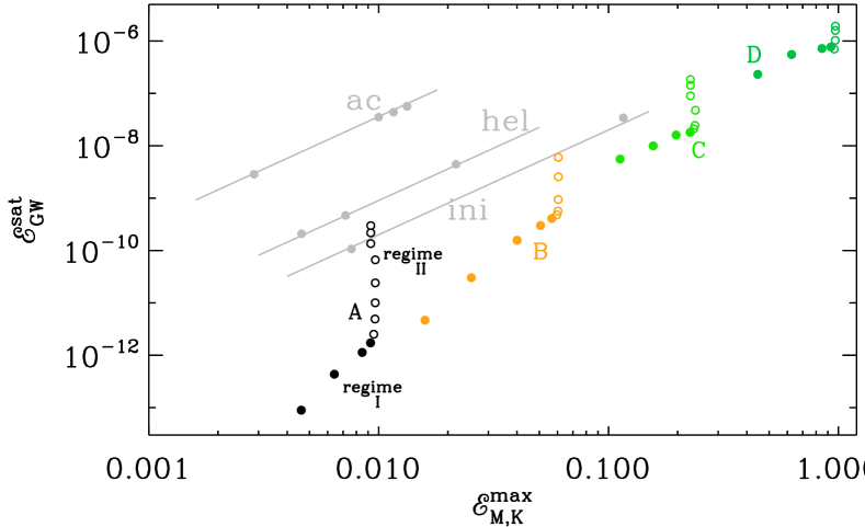
Figure 1.— ${\cal E}_{\rm GW}^{\rm sat}$ versus ${\cal E}_{\rm M}^{\max}$ for runs with ${\mu}_{50}=10^{4}$, grouped into four series with $\lambda^{1/2}=5\times 10^{4}$ (series A), $2\times 10^{4}$ (series B), $10^{4}$ (series C), and $5\times 10^{3}$ (series D). In each series we vary $\eta$. Closed (open) circles refer to cases where $v_{\mu}/v_{\lambda}<1$ ($>1$), corresponding to regime I (II). For orientation, the data of Roper Pol et al. (2020b) are shown in gray; ‘ac’ – acoustic, ‘hel’ – helically forced MHD, ‘ini’ – turbulent initial MHD state (no forcing).

Table 1 Summary of Runs from series A–G.

Run $\eta$ $\lambda^{1/2}$ ${\mu}_{50}$ $\eta k_{1}$ $v_{\mu}$ $v_{\lambda}$ $\eta{\mu}_{50}^{2}$ $k_{1}$ $k_{\lambda}$ ${\cal E}_{\rm M}^{\max}$ ${\cal E}_{\rm GW}^{\rm sat}$ $q$ A1 $1\times 10^{-6}$ $5\times 10^{4}$ $10^{4}$ $1\times 10^{-4}$ $0.01$ $0.2$ $100$ $100$ $2000$ $4.6\times 10^{-3}$ $8.9\times 10^{-14}$ $0.032$ A2 $2\times 10^{-6}$ $5\times 10^{4}$ $10^{4}$ $2\times 10^{-4}$ $0.02$ $0.2$ $200$ $100$ $4000$ $6.4\times 10^{-3}$ $4.3\times 10^{-13}$ $0.10$ A3 $5\times 10^{-6}$ $5\times 10^{4}$ $10^{4}$ $5\times 10^{-4}$ $0.05$ $0.2$ $500$ $100$ $(10000)$ $8.5\times 10^{-3}$ $1.1\times 10^{-12}$ $0.31$ A4 $1\times 10^{-5}$ $5\times 10^{4}$ $10^{4}$ $1\times 10^{-3}$ $0.1$ $0.2$ $1000$ $100$ — $9.2\times 10^{-3}$ $1.7\times 10^{-12}$ $0.71$ 167mm.5pt.7pt 2pt A5 $2\times 10^{-5}$ $5\times 10^{4}$ $10^{4}$ $2\times 10^{-3}$ $0.2$ $0.2$ $2000$ $100$ — $9.5\times 10^{-3}$ $2.5\times 10^{-12}$ $1.7$ A6 $5\times 10^{-5}$ $5\times 10^{4}$ $10^{4}$ $5\times 10^{-3}$ $0.5$ $0.2$ $5000$ $100$ — $9.6\times 10^{-3}$ $4.9\times 10^{-12}$ $2.3$ A7 $1\times 10^{-4}$ $5\times 10^{4}$ $10^{4}$ $1\times 10^{-2}$ $1$ $0.2$ $10000$ $100$ — $9.7\times 10^{-3}$ $1.0\times 10^{-11}$ $3.3$ A8 $2\times 10^{-4}$ $5\times 10^{4}$ $10^{4}$ $2\times 10^{-2}$ $2$ $0.2$ $20000$ $100$ — $9.7\times 10^{-3}$ $2.4\times 10^{-11}$ $5.1$ A9 $5\times 10^{-4}$ $5\times 10^{4}$ $10^{4}$ $5\times 10^{-2}$ $5$ $0.2$ $50000$ $100$ — $9.7\times 10^{-3}$ $6.6\times 10^{-11}$ $8.4$ A10 $1\times 10^{-3}$ $5\times 10^{4}$ $10^{4}$ $5\times 10^{-2}$ $10$ $0.2$ $1\times 10^{5}$ $50$ — $9.2\times 10^{-3}$ $1.4\times 10^{-10}$ $12$ A11 $2\times 10^{-3}$ $5\times 10^{4}$ $10^{4}$ $1\times 10^{-1}$ $20$ $0.2$ $2\times 10^{5}$ $50$ — $9.2\times 10^{-3}$ $2.2\times 10^{-10}$ $15$ A12 $5\times 10^{-3}$ $5\times 10^{4}$ $10^{4}$ $2\times 10^{-1}$ $50$ $0.2$ $5\times 10^{5}$ $50$ — $9.2\times 10^{-3}$ $3.0\times 10^{-10}$ $18$ B1 $1\times 10^{-6}$ $2\times 10^{4}$ $10^{4}$ $1\times 10^{-4}$ $0.01$ $0.5$ $100$ $100$ $800$ $1.6\times 10^{-2}$ $4.7\times 10^{-12}$ $0.027$ B2 $2\times 10^{-6}$ $2\times 10^{4}$ $10^{4}$ $2\times 10^{-4}$ $0.02$ $0.5$ $200$ $100$ $1600$ $2.5\times 10^{-2}$ $3.0\times 10^{-11}$ $0.087$ B3 $5\times 10^{-6}$ $2\times 10^{4}$ $10^{4}$ $5\times 10^{-4}$ $0.05$ $0.5$ $500$ $100$ $4000$ $4.0\times 10^{-2}$ $1.6\times 10^{-10}$ $0.31$ B4 $1\times 10^{-5}$ $2\times 10^{4}$ $10^{4}$ $1\times 10^{-3}$ $0.1$ $0.5$ $1000$ $100$ $(8000)$ $5.1\times 10^{-2}$ $3.0\times 10^{-10}$ $0.68$ B5 $2\times 10^{-5}$ $2\times 10^{4}$ $10^{4}$ $2\times 10^{-3}$ $0.2$ $0.5$ $2000$ $100$ — $5.7\times 10^{-2}$ $4.1\times 10^{-10}$ $1.4$ 167mm.5pt.7pt 2pt B6 $5\times 10^{-5}$ $2\times 10^{4}$ $10^{4}$ $5\times 10^{-3}$ $0.5$ $0.5$ $5000$ $100$ — $6.0\times 10^{-2}$ $4.8\times 10^{-10}$ $3.7$ B7 $1\times 10^{-4}$ $2\times 10^{4}$ $10^{4}$ $1\times 10^{-2}$ $1$ $0.5$ $10000$ $100$ — $6.0\times 10^{-2}$ $5.6\times 10^{-10}$ $3.9$ B8 $2\times 10^{-4}$ $2\times 10^{4}$ $10^{4}$ $2\times 10^{-2}$ $2$ $0.5$ $20000$ $100$ — $6.0\times 10^{-2}$ $9.4\times 10^{-10}$ $5.1$ B9 $5\times 10^{-4}$ $2\times 10^{4}$ $10^{4}$ $5\times 10^{-2}$ $5$ $0.5$ $50000$ $100$ — $6.0\times 10^{-2}$ $2.6\times 10^{-9}$ $8.4$ B10 $1\times 10^{-3}$ $2\times 10^{4}$ $10^{4}$ $1\times 10^{-1}$ $10$ $0.5$ $1\times 10^{5}$ $100$ — $6.0\times 10^{-2}$ $6.0\times 10^{-9}$ $12$ C1 $5\times 10^{-6}$ $10^{4}$ $10^{4}$ $5\times 10^{-4}$ $0.05$ $1$ $500$ $100$ $2000$ $1.1\times 10^{-1}$ $5.6\times 10^{-9}$ $0.33$ C2 $1\times 10^{-5}$ $10^{4}$ $10^{4}$ $1\times 10^{-3}$ $0.1$ $1$ $1000$ $100$ $4000$ $1.6\times 10^{-1}$ $9.9\times 10^{-9}$ $0.64$ C3 $2\times 10^{-5}$ $10^{4}$ $10^{4}$ $2\times 10^{-3}$ $0.2$ $1$ $2000$ $100$ $(8000)$ $2.0\times 10^{-1}$ $1.6\times 10^{-8}$ $1.3$ C4 $5\times 10^{-5}$ $10^{4}$ $10^{4}$ $5\times 10^{-3}$ $0.5$ $1$ $5000$ $100$ — $2.3\times 10^{-1}$ $1.8\times 10^{-8}$ $3.0$ 167mm.5pt.7pt 2pt C5 $1\times 10^{-4}$ $10^{4}$ $10^{4}$ $1\times 10^{-2}$ $1$ $1$ $10000$ $100$ — $2.3\times 10^{-1}$ $2.1\times 10^{-8}$ $6.2$ C6 $2\times 10^{-4}$ $10^{4}$ $10^{4}$ $2\times 10^{-2}$ $2$ $1$ $20000$ $100$ — $2.4\times 10^{-1}$ $2.4\times 10^{-8}$ $6.6$ C7 $5\times 10^{-4}$ $10^{4}$ $10^{4}$ $5\times 10^{-2}$ $5$ $1$ $50000$ $100$ — $2.4\times 10^{-1}$ $4.8\times 10^{-8}$ $9.1$ C8 $1\times 10^{-3}$ $10^{4}$ $10^{4}$ $5\times 10^{-2}$ $10$ $1$ $1\times 10^{5}$ $50$ — $2.3\times 10^{-1}$ $9.0\times 10^{-8}$ $13$ C9 $2\times 10^{-3}$ $10^{4}$ $10^{4}$ $1\times 10^{-1}$ $20$ $1$ $2\times 10^{5}$ $50$ — $2.3\times 10^{-1}$ $1.4\times 10^{-7}$ $16$ C10 $5\times 10^{-3}$ $10^{4}$ $10^{4}$ $2\times 10^{-1}$ $50$ $1$ $5\times 10^{5}$ $50$ — $2.3\times 10^{-1}$ $1.8\times 10^{-7}$ $18$ D1 $1\times 10^{-5}$ $5\times 10^{3}$ $10^{4}$ $2\times 10^{-3}$ $0.1$ $2$ $1000$ $200$ $2000$ $4.5\times 10^{-1}$ $2.3\times 10^{-7}$ $0.54$ D2 $2\times 10^{-5}$ $5\times 10^{3}$ $10^{4}$ $2\times 10^{-3}$ $0.2$ $2$ $2000$ $100$ $4000$ $6.3\times 10^{-1}$ $5.5\times 10^{-7}$ $1.2$ D3 $5\times 10^{-5}$ $5\times 10^{3}$ $10^{4}$ $5\times 10^{-3}$ $0.5$ $2$ $5000$ $100$ $(10000)$ $8.5\times 10^{-1}$ $7.2\times 10^{-7}$ $2.5$ D4 $1\times 10^{-4}$ $5\times 10^{3}$ $10^{4}$ $1\times 10^{-2}$ $1$ $2$ $10000$ $100$ — $9.3\times 10^{-1}$ $7.7\times 10^{-7}$ $4.7$ 167mm.5pt.7pt 2pt D5 $2\times 10^{-4}$ $5\times 10^{3}$ $10^{4}$ $4\times 10^{-2}$ $2$ $2$ $20000$ $200$ — $9.6\times 10^{-1}$ $7.0\times 10^{-7}$ $8.7$ D6 $5\times 10^{-4}$ $5\times 10^{3}$ $10^{4}$ $1\times 10^{-1}$ $5$ $2$ $50000$ $200$ — $9.7\times 10^{-1}$ $1.0\times 10^{-6}$ $10$ D7 $1\times 10^{-3}$ $5\times 10^{3}$ $10^{4}$ $2\times 10^{-1}$ $10$ $2$ $1\times 10^{5}$ $200$ — $9.7\times 10^{-1}$ $1.6\times 10^{-6}$ $12$ D8 $2\times 10^{-3}$ $5\times 10^{3}$ $10^{4}$ $4\times 10^{-1}$ $20$ $2$ $2\times 10^{5}$ $200$ — $9.7\times 10^{-1}$ $1.9\times 10^{-6}$ $14$ E1 $5\times 10^{-6}$ $10^{4}$ $2\times 10^{4}$ $1\times 10^{-3}$ $0.1$ $2$ $2000$ $200$ $4000$ $4.4\times 10^{-1}$ $8.6\times 10^{-8}$ $0.67$ E2 $1\times 10^{-5}$ $10^{4}$ $2\times 10^{4}$ $2\times 10^{-3}$ $0.2$ $2$ $4000$ $200$ $8000$ $6.3\times 10^{-1}$ $1.5\times 10^{-7}$ $1.2$ E3 $2\times 10^{-5}$ $10^{4}$ $2\times 10^{4}$ $4\times 10^{-3}$ $0.4$ $2$ $8000$ $200$ $(16000)$ $8.1\times 10^{-1}$ $1.9\times 10^{-7}$ $2.2$ E4 $5\times 10^{-5}$ $10^{4}$ $2\times 10^{4}$ $1\times 10^{-2}$ $1$ $2$ $20000$ $200$ — $9.3\times 10^{-1}$ $2.0\times 10^{-7}$ $4.9$ 167mm.5pt.7pt 2pt E5 $1\times 10^{-4}$ $10^{4}$ $2\times 10^{4}$ $2\times 10^{-2}$ $2$ $2$ $40000$ $200$ — $9.6\times 10^{-1}$ $2.1\times 10^{-7}$ $9.6$ E6 $2\times 10^{-4}$ $10^{4}$ $2\times 10^{4}$ $4\times 10^{-2}$ $4$ $2$ $80000$ $200$ — $9.7\times 10^{-1}$ $2.6\times 10^{-7}$ $10$ E7 $5\times 10^{-4}$ $10^{4}$ $2\times 10^{4}$ $1\times 10^{-1}$ $10$ $2$ $2\times 10^{5}$ $200$ — $9.7\times 10^{-1}$ $4.6\times 10^{-7}$ $13$ E8 $1\times 10^{-3}$ $10^{4}$ $2\times 10^{4}$ $2\times 10^{-1}$ $20$ $2$ $4\times 10^{5}$ $200$ — $9.7\times 10^{-1}$ $6.2\times 10^{-7}$ $16$ F1 $5\times 10^{-6}$ $10^{3}$ $2\times 10^{3}$ $2\times 10^{-4}$ $0.01$ $2$ $20$ $50$ $40$ $9.4\times 10^{-2}$ $7.2\times 10^{-11}$ $0.00091$ F2 $1\times 10^{-5}$ $10^{3}$ $2\times 10^{3}$ $5\times 10^{-4}$ $0.02$ $2$ $40$ $50$ $80$ $1.4\times 10^{-1}$ $6.7\times 10^{-9}$ $0.012$ F3 $2\times 10^{-5}$ $10^{3}$ $2\times 10^{3}$ $1\times 10^{-3}$ $0.04$ $2$ $80$ $50$ $160$ $2.5\times 10^{-1}$ $1.7\times 10^{-7}$ $0.067$ F4 $5\times 10^{-5}$ $10^{3}$ $2\times 10^{3}$ $1\times 10^{-3}$ $0.1$ $2$ $200$ $25$ $400$ $4.5\times 10^{-1}$ $3.3\times 10^{-6}$ $0.41$ F5 $1\times 10^{-4}$ $10^{3}$ $2\times 10^{3}$ $2\times 10^{-3}$ $0.2$ $2$ $400$ $25$ $800$ $6.3\times 10^{-1}$ $8.2\times 10^{-6}$ $0.91$ F6 $2\times 10^{-4}$ $10^{3}$ $2\times 10^{3}$ $5\times 10^{-3}$ $0.4$ $2$ $800$ $25$ $(1600)$ $8.1\times 10^{-1}$ $1.3\times 10^{-5}$ $1.8$ F7 $5\times 10^{-4}$ $10^{3}$ $2\times 10^{3}$ $1\times 10^{-2}$ $1$ $2$ $2000$ $25$ — $9.3\times 10^{-1}$ $1.6\times 10^{-5}$ $4.3$ 167mm.5pt.7pt 2pt F8 $1\times 10^{-3}$ $10^{3}$ $2\times 10^{3}$ $2\times 10^{-2}$ $2$ $2$ $4000$ $25$ — $9.6\times 10^{-1}$ $1.8\times 10^{-5}$ $8.9$ G1 $1\times 10^{-5}$ $5\times 10^{2}$ $10^{3}$ $2\times 10^{-4}$ $0.01$ $2$ $10$ $25$ $20$ $9.8\times 10^{-2}$ $1.1\times 10^{-10}$ $0.00054$ G2 $2\times 10^{-5}$ $5\times 10^{2}$ $10^{3}$ $5\times 10^{-4}$ $0.02$ $2$ $20$ $25$ $40$ $1.5\times 10^{-1}$ $7.5\times 10^{-9}$ $0.0060$ G3 $5\times 10^{-5}$ $5\times 10^{2}$ $10^{3}$ $1\times 10^{-3}$ $0.05$ $2$ $50$ $25$ $100$ $2.9\times 10^{-1}$ $6.0\times 10^{-7}$ $0.066$ G4 $1\times 10^{-4}$ $5\times 10^{2}$ $10^{3}$ $2\times 10^{-3}$ $0.1$ $2$ $100$ $25$ $200$ $4.5\times 10^{-1}$ $4.8\times 10^{-6}$ $0.24$ G5 $2\times 10^{-4}$ $5\times 10^{2}$ $10^{3}$ $5\times 10^{-3}$ $0.2$ $2$ $200$ $25$ $400$ $6.3\times 10^{-1}$ $1.6\times 10^{-5}$ $0.63$ G6 $5\times 10^{-4}$ $5\times 10^{2}$ $10^{3}$ $1\times 10^{-2}$ $0.5$ $2$ $500$ $25$ $(1000)$ $8.6\times 10^{-1}$ $3.9\times 10^{-5}$ $1.8$ G7 $1\times 10^{-3}$ $5\times 10^{2}$ $10^{3}$ $1\times 10^{-2}$ $1$ $2$ $1000$ $10$ — $9.3\times 10^{-1}$ $5.4\times 10^{-5}$ $4.0$ 167mm.5pt.7pt 2pt G8 $2\times 10^{-3}$ $5\times 10^{2}$ $10^{3}$ $2\times 10^{-2}$ $2$ $2$ $2000$ $10$ — $9.6\times 10^{-1}$ $6.2\times 10^{-5}$ $8.2$

Note: Dotted lines separate regime I from regime II runs. Bracketed $k_{\lambda}$ values and hyphens mean that $k_{\lambda}$ exceeds $k_{\mu}$.

In view of any type of driven or decaying MHD turbulence, the dependence of ${\cal E}_{\rm GW}^{\rm sat}$ on $\eta$ seems not very intuitive as we find it to increase with increasing $\eta$ although one would have expected that smaller $\eta$ would cause a more vigorous time dependence. However, the increase of ${\cal E}_{\rm GW}^{\rm sat}$ with $\eta$ is plausible due to the fact that the maximum growth rate of $\bm{B}$ is proportional to $\eta$ – a specific of the CME.

In all of our simulations of series A–D, the parameter $q$ is even lower than in the least efficient simulations of Roper Pol et al. (2020b). This is rather surprising and might indicate that the turbulence from the CME has a much less vigorous time dependence than the cases considered there. For understanding the reason behind this, it is necessary to study the present results in more detail by inspecting the magnetic and GW energy spectra. We begin by analyzing their mutual relation at late times when the magnetic energy has already reached a maximum and the GW energy has achieved a steady state.

3.2. Late time GW spectra from the CME

We consider the case $\eta=10^{-6}$, $\lambda=4\times 10^{8}$, and ${\mu}_{50}=10^{4}$, which corresponds to Run B1. This means that $v_{\mu}=0.01$ and $v_{\lambda}=0.5$, so $v_{\lambda}/v_{\mu}=50$, and we are clearly in regime I.

The CME leads to exponential magnetic field generation, followed by subsequent turbulent decay. At the time of the magnetic maximum, an approximate $k^{-2}$ magnetic energy spectrum with a short inertial range develops (Brandenburg et al., 2017b). We then expect a $k^{-4}$ spectrum for the GW energy and a $k^{-6}$ spectrum for ${\sf h}$; see Roper Pol et al. (2020b). There is a trend for this to happen also in the present case, although ${\cal E}_{\rm GW}(k)$ does not have clear power law subranges; see Figure 2. This is because the turbulence is not steady and both energy spectra look very different even just shortly before the magnetic field saturates, as will be shown below.

Figure 2.— Magnetic and GW energy spectra for Run B1 with ${\mu}_{50}=10^{4}$, $\lambda=4\times 10^{8}$, and $\eta=10^{-6}$, which is in regime I with $(v_{\mu}=0.01)<(v_{\lambda}=0.5)$. $E_{\rm M}(k)$ (red) is shown at the time of magnetic maximum (solid, $t=1.92$), the time when the $k^{-2}$ spectrum is most clear ($t=3$, dashed), and at selected other times (dotted, $t=1.71$, $1.77$, $1.83$, $1.89$, $1.94$, $2.00$, $2.15$, $2.32$, $2.52$, $2.74$, and $3.00$, while $E_{\rm GW}(k)$ (solid blue) is from the simulation’s end time ($t=14$), when it can be approximated by $k^{2}\mbox{\rm Sp}(\mbox{\boldmath${\sf h}$}{})/6$ (dashed-dotted blue). The black horizontal dashed-dotted line marks the saturation limit of Equation (10), ${\mu}_{50}/\lambda$, and the vertical dashed line marks the position of $k_{\mu}$.

Figure 3.— Similar to Figure 2, but for Run B10 with $\eta=10^{-3}$, which is in regime II with $(v_{\mu}=10)>(v_{\lambda}=0.5)$. $E_{\rm M}(k)$ (solid red) is at the time when the magnetic energy has attained its maximum ($t=1.001$), dotted red lines show $E_{\rm M}(k)$ at $t=1.0008$, $1.003$, $1.008$, $1.024$, and $1.075$, while $E_{\rm GW}(k)$ is from the simulation’s end time ($t=1.075$), when $E_{\rm GW}(k)\approx k^{2}\mbox{\rm Sp}(\mbox{\boldmath${\sf h}$}{})/6$.

For runs in regime II, however, we find an approximate $k^{-0.5}$ profile for $E_{\rm GW}(k)$; see Figure 3. This is closer to the case of stationary turbulence; see Table LABEL:Tregimes for a comparison of some characteristic properties. $E_{\rm M}(k)$ shows an approximate $k^{5}$ subinertial range. This is steeper than the $k^{4}$ spectrum expected based on causality arguments (Durrer & Caprini, 2003). However, as we will see later more clearly, at early times and close to $k=k_{\mu}$ the magnetic energy spectra show a dent, explaining therefore the apparent steeper spectrum at early times; a $k^{4}$ subinertial range can still be identified at other times. In particular, for fully helical magnetic fields, a $k^{4}$ spectrum spectrum always emerges, regardless of the initial slope; see Figure 3(a) of Brandenburg & Kahniashvili (2017).

Table 2 Spectral properties of GWs in regimes I, II, and in stationary turbulence.

	Run B1	Run B10	Stationary
	Regime I	Regime II	turbulence∗
$\mbox{\rm Sp}(\dot{\mbox{\boldmath${\sf h}$}{}})/\mbox{\rm Sp}(\mbox{\boldmath${\sf h}$}{})$	$0.89\,(2\gamma_{0})^{2}$	$0.96\,(2\gamma_{0})^{2}$	$0.30\,k_{\rm f}^{2}$
$\mbox{\rm Sp}(\mbox{\boldmath${\sf T}$}{})/\mbox{\rm Sp}(\dot{\mbox{\boldmath${\sf h}$}{}})$	$1.1\,(2\gamma_{0}{\mu}_{50})^{2}$	$0.98\,(2\gamma_{0})^{2}$	$0.10\,k_{\rm f}^{2}$
$\mbox{\rm Sp}(\mbox{\boldmath${\sf h}$}{})$, kinematic	$k^{-2}$	$k^{2}$	—
$\mbox{\rm Sp}(\mbox{\boldmath${\sf h}$}{})$, saturated	$k^{-2}$	$k^{-0.5}$	$k^{0}$

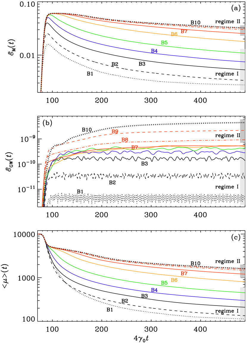
Figure 4.— Evolution of ${\cal E}_{\rm M}$, ${\cal E}_{\rm GW}$, and $\langle{\mu}_{5}\rangle$ for Runs B1–B10. The light and dark gray bars on the right of each panel indicate regimes I and II, respectively. Note the occurrence of a slow final saturation phase of ${\cal E}_{\rm GW}$ for all runs in regime II (Runs B7–B10). Run 8 (red dashed-dotted line), Run 9 (red dashed line), and Run 10 (upper black dotted line) overlap in ${\cal E}_{\rm M}$ and $\langle{\mu}_{5}\rangle$, but are well separated in ${\cal E}_{\rm GW}$.

3.3. GW spectra during the early growth phase

At early times, as discussed above, ${\cal E}_{\rm M}(t)$ grows exponentially at a rate $2\gamma_{0}=\eta{\mu}_{50}^{2}/2$ and ${\cal E}_{\rm GW}(t)$ grows at a rate $4\gamma_{0}$. Across the different runs, this rate varies by three orders of magnitude. To compare the evolution of GW and magnetic energies for the different runs, it is thus convenient to plot both quantities versus $4\gamma_{0}t$. The result is shown in Figure 4 for the runs of series B. One clearly sees a slow final saturation phase of ${\cal E}_{\rm GW}(t)$ for all runs in regime II (Runs B7–B10), while ${\cal E}_{\rm M}(t)$ and $\langle{\mu}_{5}\rangle(t)$ are almost unchanged across different runs. During the exponential growth phase, ${\mu}_{5}$ is close to its initial value, ${\mu}_{50}=10^{4}$. It drops fastest in regime I, where $\eta$ is small (Runs B1–B5). However, in contrast to Figure 1, where we saw a marked qualitative change as we move from regime I to regime II, no such change is seen in Figure 4 between regime I (Runs B1–B5) and II (Runs B7–B10).

In the case of stationary GW spectra (see, e.g., Kahniashvili et al., 2021), and also in the previous section, we always have $\mbox{\rm Sp}(\dot{\mbox{\boldmath${\sf h}$}{}})\approx k^{2}\mbox{\rm Sp}(\mbox{\boldmath${\sf h}$}{})\approx k^{-2}\mbox{\rm Sp}(\mbox{\boldmath${\sf T}$}{})$, but this is not so in the early exponential growth phase. Nevertheless, in both these regimes, we find $\mbox{\rm Sp}(\mbox{\boldmath${\sf T}$}{})\propto k^{2}$. This is a consequence of the almost monochromatic magnetic field generation in a narrow range around $k=k_{\mu}$, which implies that the spectral slope of $E_{\rm M}(k)$ for $k<k_{\mu}$ is always steeper than that of white noise ($\propto k^{2}$), so we call it “blue noise”. However, the square of a field with a blue noise spectrum always has a white noise spectrum (Brandenburg & Boldyrev, 2020). This explains why $\mbox{\rm Sp}(\mbox{\boldmath${\sf T}$}{})\propto k^{2}$.

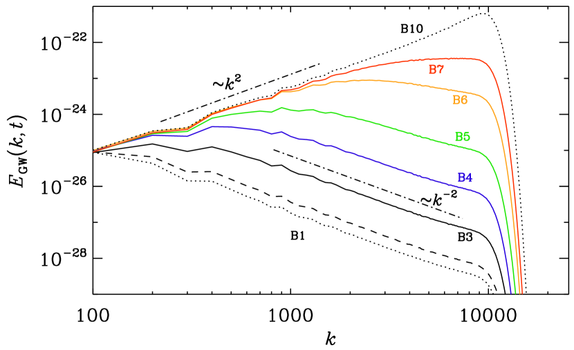
Figure 5.— Comparison of GW energy spectra during the kinematic growth stage for runs in regime I (B1–B5) and regime II (B7–B10). Note the change of slope at a certain wavenumber that increases as we go from regime I to regime II.

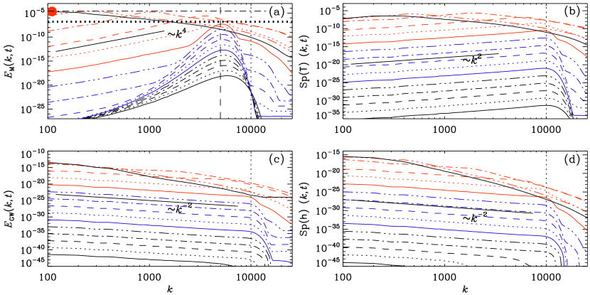
Figure 6.— Time-evolving magnetic and GW energy spectra along with spectra of stress ${\sf T}$ and strain ${\sf h}$ for Run B1 (regime I) at $t-1=0.2$, $0.25$, $0.3$, $0.35$, $0.4$ in black, $0.45$, $0.5$, $0.55$, $0.6$, $0.65$ in blue, $0.7$, $0.75$, $0.8$, $0.9$, $1.4$ in red, and the time of maximum ${\cal E}_{\rm M}$ at $1.9$, again in black. In panel (a), the dotted horizontal line marks the level of $C_{5}{\mu}_{50}\eta^{2}$, and the horizontal dashed-dotted line the level of $C_{\lambda}{\mu}_{50}/\lambda$. Vertical dotted and dashed lines mark the positions of $2k_{\mu}={\mu}_{50}$ and $k_{\mu}$, respectively. The red filled symbol denotes the peak of $E_{\rm M}(k)$ at the time of the magnetic maximum.

Figure 7.— Similar to Figure 6, but for Run B10 with $\eta=10^{-3}$, which is in regime II with $(v_{\mu}=10)>(v_{\lambda}=0.5)$, at $t-1=2$, $3$, $4$, $5$, $6\times 10^{-4}$ in black, $6.5$, $7$, $7.5$, $8$, $9\times 10^{-4}$ in blue, and $0.001$ (maximum ${\cal E}_{\rm M}$), $0.002$, $0.007$, and $0.0075$ in red. ${\cal E}_{\rm M}(t)$ reaches a maximum at $t-1=1.1\times 10^{-3}$ and ${\cal E}_{\rm GW}(t)$ at $t-1=0.02$. The upward arrow in panel (c) emphasizes the change in slope.

To see how the transition from a $k^{-2}$ profile for small $k$ toward a $k^{2}$ profile for large $k$ occurs in $E_{\rm GW}(k)$, we plot it in Figure 5 during the kinematic growth phase. The times have been arranged such that all spectra coincide at $k=k_{1}\equiv 100$. We clearly see the emergence of a breakpoint from a $k^{2}$ spectrum at low $k$ toward a $k^{-2}$ spectrum at larger $k$. The breakpoint shifts toward larger wavenumbers as we go from regime I to regime II, although it can no longer be identified for Runs B7–B10.

Furthermore, in both regimes I and II, we find $\mbox{\rm Sp}(\dot{\mbox{\boldmath${\sf h}$}{}})\propto\mbox{\rm Sp}(\mbox{\boldmath${\sf h}$}{})$ during the early growth phase, but their slopes are different in the two regimes. In Figures 6 and 7, we compare the spectra for Runs B1 (regime I) and B10 (regime II), including magnetic and GW energy spectra along with the spectra of stress and strain. We clearly see that at early times, $\mbox{\rm Sp}(\mbox{\boldmath${\sf h}$}{})$ and $\mbox{\rm Sp}(\dot{\mbox{\boldmath${\sf h}$}{}})=6{\cal E}_{\rm GW}(k)$ all have the same slope proportional to $k^{-2}$ and $k^{2}$ in regimes I and II, respectively. Specifically, at $k=k_{\mu}$, we find for the ratio $\mbox{\rm Sp}(\dot{\mbox{\boldmath${\sf h}$}{}})/\mbox{\rm Sp}(\mbox{\boldmath${\sf h}$}{})\approx(2\gamma_{0})^{2}$ in both regimes. It is important to emphasize that, even though $\gamma(k)$ depends on $k$, the stress spectrum grows at the maximum rate $\gamma_{0}$ at all $k$. For $k\leq k_{\mu}$, this can simply be understood as a consequence of the result of Brandenburg & Boldyrev (2020) that the square of a field with a blue noise spectrum always has a white noise spectrum.

For $k>{\mu}_{50}$, the magnetic energy spectrum always drops rapidly. Based again on the results of Brandenburg & Boldyrev (2020), since the spectrum is here a red one, the magnetic stress spectrum also drops rapidly with the same slope. Following Brandenburg & Boldyrev (2020), in the range $k_{\mu}<k<{\mu}_{50}$ the spectrum is slightly shallower than $k^{2}$ and it peaks approximately at $k={\mu}_{50}$.

In Table LABEL:Tregimes, we summarize the spectral properties during the early kinematic growth phase and contrast it with the saturated phase. In regime I, we also find $\mbox{\rm Sp}(\mbox{\boldmath${\sf T}$}{})/\mbox{\rm Sp}(\dot{\mbox{\boldmath${\sf h}$}{}})\approx(2\gamma_{0})^{2}$, but in regime II, there is an extra ${\mu}_{50}^{2}$ factor (see Table LABEL:Tregimes), which is a consequence of the different slopes of both curves. The reason for the change of slopes in regimes I and II is explained in the next section.

3.4. Difference in the slopes between regimes I and II

To understand the change in the spectral slopes between regimes I and II during the kinematic growth stage it is convenient to restrict our attention to the case of a purely monochromatic exponential growth of $\bm{B}$ at the wavenumber $k_{\mu}$ with the rate $\gamma_{0}=\eta{\mu}_{50}^{2}/4$. As explained in Section 3.3, the magnetic stress increases then at all $k$ at the rate $2\gamma_{0}$; see also Figures 6 and 7 for a direct confirmation of this property.

Let us now assume that $\tilde{T}(\bm{k},t)$, representing the Fourier transform of one of the two polarization modes of the stress, $T_{+}$ and $T_{\times}$, is given by

$$\tilde{T}(\bm{k},t)=\theta(t-1)\,\tilde{T}_{0}(k)\,e^{2\gamma_{0}(t-1)},$$ (16)

where $\theta(t)$ is the Heaviside step function, and $\tilde{T}_{0}(k)$ is assumed to depend just on $k=|\bm{k}|$.

Using $\tilde{h}(k,1)=\dot{\tilde{h}}(k,1)=0$ as initial conditions, we can solve Equation (5) during the early growth phase in closed form as

$$\tilde{h}(k,t)=\frac{6\tilde{T}_{0}(k)}{4\gamma_{0}^{2}+k^{2}}\left[e^{2\gamma_{0}\tau}-\cos k\tau-\frac{2\gamma_{0}}{k}\sin k\tau\right]_{\tau=t-1},$$ (17)

where $\tilde{h}$ stands for either $\tilde{h}_{+}$ or $\tilde{h}_{\times}$. In practice, we are always interested in the case where the exponential term dominates over the cosine and sine terms. When $k\ll 2\gamma_{0}$, $\mbox{\rm Sp}(h)$ and $\mbox{\rm Sp}(\dot{h})$ are proportional to $\mbox{\rm Sp}(T_{0})$. In particular, when $\tilde{T}_{0}(k)$ is a white noise spectrum, we have $\mbox{\rm Sp}(h)\propto k^{2}|\tilde{T}_{0}(k)|^{2}\propto k^{2}$. However, when $k\gg 2\gamma_{0}$, we find $\mbox{\rm Sp}(h)\propto\mbox{\rm Sp}(\dot{h})\propto k^{2}|\tilde{T}_{0}(k)/k^{2}|^{2}\propto k^{-2}$, with the breakpoint being at $k_{0}=2\gamma_{0}$.

To compare with the results of our simulations, let us try to numerically determine the breakpoint $k=k_{\rm GW}$ as

$$k_{\rm GW}^{-1}=\int k^{-1}E_{\rm GW}(k)\,{\rm d}{}k\,\left/\int E_{\rm GW}(k)\,{\rm d}{}k\right..$$ (18)

We have calculated it for the models of series B and D and find that our analytic prediction $k_{0}=2\gamma_{0}$ matches the numerical results rather well; see Figure 8. Representing $\mbox{\rm Sp}(\dot{h})$ according to Equation (17) by

$$E_{\rm GW}^{\rm model}\propto\left[\frac{k}{k_{0}^{2}+k^{2}}\,e^{-(k/{\mu}_{50})^{4}}\right]^{2},$$ (19)

where the exponential factor is intended to model the cutoff near $k={\mu}_{50}$, we find $k_{\rm GW}=(\pi/2)\,k_{0}$, which is why we have compensated $k_{\rm GW}$ in Figure 8 by this value. The reason why there are departures for small and large values of $\eta{\mu}_{50}^{2}$ is that the wavenumber range used for the integration is limited. In addition to estimating $k_{0}$ as $k_{\rm GW}$ from Equation (18), we compute a fit to the model spectrum of Equation (19). We do this by minimizing the mean squared difference between the actual spectrum and the model spectrum. Those results are also shown in Figure 8 (open symbols).

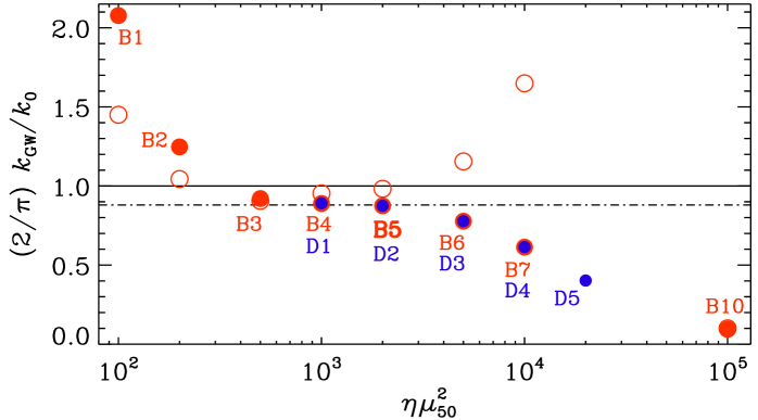
Figure 8.— Dependence of $k_{\rm GW}$ from Equation (18), normalized by $k_{0}\pi/2$, on $\eta{\mu}_{50}^{2}$ for runs of series B (red filled symbols) and D (blue filled symbols). Run B5 is highlighted in boldface (cf. Figure 9). The dashed-dotted line gives an approximate fit through the data points near their plateau, and the solid line goes through unity, the theoretically expected value. The red open symbols denote the values of $k_{0}$ obtained by fitting the spectra of Figure 5 to the model spectrum of Equation (19), similar to what is done in Figure 9.

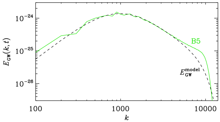
Figure 9.— Comparison of the GW energy spectrum for Run B5 and the model spectrum of Equation (19).

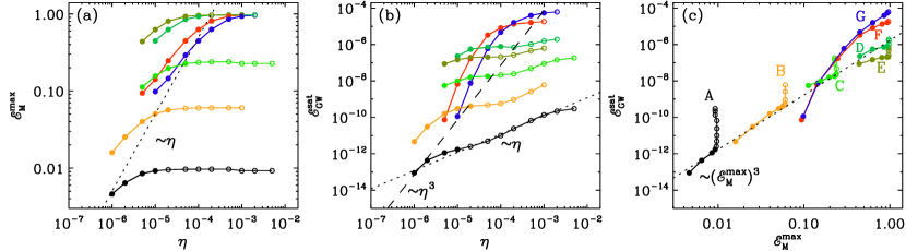
Figure 10.— Dependence of ${\cal E}_{\rm M}^{\rm max}$ and ${\cal E}_{\rm GW}^{\rm sat}$ on $\eta$, and their mutual parametric dependence for runs of series A–D with ${\mu}_{50}=10^{4}$ and $\lambda^{1/2}=5\times 10^{4}$, $2\times 10^{4}$, $10^{4}$, $5\times 10^{3}$, respectively, series E with ${\mu}_{50}=2\times 10^{4}$, $\lambda^{1/2}=10^{4}$, series F with ${\mu}_{50}=2000$, $\lambda^{1/2}=1000$, and series G with ${\mu}_{50}=1000$, $\lambda^{1/2}=100$. Filled (open) symbols denote runs in regime I (II). The dotted line in panel (c) is for $q=13\,({\cal E}_{\rm M}^{\rm max})^{1/2}$.

In Figure 9, we show a comparison of one of the GW energy spectra of Figure 5 with Equation (19). While it provides an excellent description of $E_{\rm GW}(k)$ in the bulk of the $k$ range, the exponential factor is not sharp enough to model the simulation data near the cutoff.

3.5. Change of slope toward late times

We see in Figure 4(b) that for all runs in regime I, ${\cal E}_{\rm GW}$ saturates quickly after ${\cal E}_{\rm M}$ reaches its maximum, while for runs in regime II, ${\cal E}_{\rm GW}$ continues to display a slow saturation behavior. To understand this unusual behavior, we must look again at Figure 7, showing the evolution of the spectra in Run B10, which is in regime II. We see that, at the time when ${\cal E}_{\rm M}$ reaches its maximum, the peak of $E_{\rm M}(k)$ is still at $k\approx{\mu}_{5}$. After that, ${\cal E}_{\rm M}$ decays such that ${\cal E}_{\rm M}/k_{\rm M}={\rm const}{}$, so based on the earlier results of Roper Pol et al. (2020b), we would expect ${\cal E}_{\rm GW}$ to stay constant. Looking at the evolution of $E_{\rm GW}(k)$ for Run B10 near equilibration in Figure 7(c), we observe a change in slope. This could be responsible for the occurrence of a slow final saturation phase of ${\cal E}_{\rm GW}$ for the runs in regime II, and especially for Run B10, seen in Figure 4.

To discuss this possibility quantitatively, let us assume a simplified spectrum of the form

$$E_{\rm GW}(k,t_{\rm bef})=3{\cal E}_{0}\,k^{2}/{\mu}_{50}^{3}\quad\mbox{if $k<2k_{\mu}={\mu}_{50}$}$$ (20)

for the time $t_{\rm bef}$ before the slope changes. For $k>2k_{\mu}$ we assume a sharp fall-off and therefore ignore that contribution. This $k^{2}$ spectrum is normalized such that $\int E_{\rm GW}(k,t_{\rm bef})\,{\rm d}{}k={\cal E}_{0}$. The spectrum is then assumed to change to a new power law $\propto k^{s}$, with an exponent $s$, of the form

$$E_{\rm GW}(k,t_{\rm aft})=3{\cal E}_{0}\,k^{s}/{\mu}_{50}^{s+1}$$ (21)

for the time $t_{\rm aft}$ after the slope has changed. Employing the same ${\cal E}_{0}$ in Equations (20) and (21), accounts for the fact that $E_{\rm GW}({\mu}_{50})=3{\cal E}_{0}/{\mu}_{50}$ is no longer changing in time; see Figure 7(c). For $s>-1$, the resulting GW energy is $3{\cal E}_{0}/(s+1)$. In Figure 3, we found $s=-0.5$, so the resulting GW energy is then $\approx 6{\cal E}_{0}$, which is compatible with the late-time excess of ${\cal E}_{\rm GW}$ in Run B10 relative to Run B6. It should be noted, however, that the change of slope occurs at a time when the magnetic field is about to reach the scale of the domain. It is therefore conceivable that $s=-0.5$ could be an artifact of the finite domain size. In particular, $s=0$ is what has previously been found based on numerical simulations (Roper Pol et al., 2020b) including larger domains.

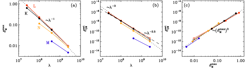
Figure 11.— Dependence of ${\cal E}_{\rm M}^{\rm max}$ and ${\cal E}_{\rm GW}^{\rm sat}$ on $\lambda$, and their mutual parametric dependence for runs of series K–N. Filled (open) symbols denote runs in regime I (II). The dotted line in panel (c) is for $q=7\,{\cal E}_{\rm M}^{\max}$.

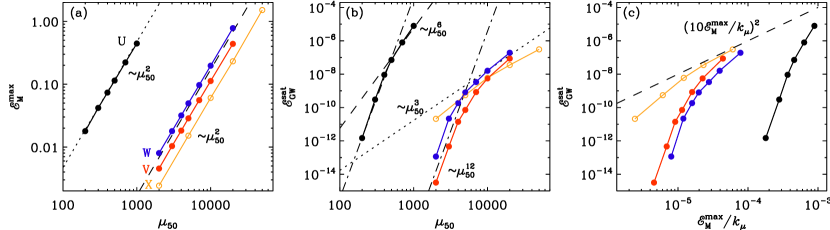
Figure 12.— Dependence of ${\cal E}_{\rm M}^{\rm max}$ and ${\cal E}_{\rm GW}^{\rm sat}$ on ${\mu}_{50}$, and their mutual parametric dependence for runs of series U–X. Filled (open) symbols denote runs in regime I (II). The dashed line in panel (c) is for $q=10$.

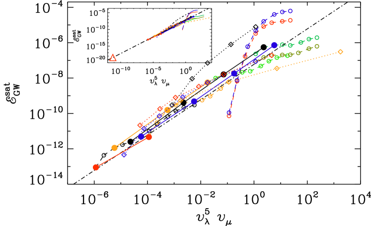
Figure 13.— Dependence of ${\cal E}_{\rm GW}^{\rm sat}$ on $v_{\lambda}^{5}v_{\mu}$ for all runs of series A–G with the same colors as in Figure 10 (dashed lines with open circles), series K–N with the same colors as in Figure 11 (solid lines with filled symbols), and series U–X with the same colors as in Figure 12 (dotted lines with diamonds). The dashed-dotted line has slope unity. The inset shows the same plot, extended down to $v_{\lambda}^{5}v_{\mu}=6\times 10^{-12}$, corresponding to the CME estimate for the early universe, and denoted by a big red triangle in the lower left.

Table 3 Summary of Runs from series K–N.

Run $\eta$ $\lambda^{1/2}$ ${\mu}_{50}$ $\eta k_{1}$ $v_{\mu}$ $v_{\lambda}$ $\eta{\mu}_{50}^{2}$ $k_{1}$ $k_{\lambda}$ ${\cal E}_{\rm M}^{\max}$ ${\cal E}_{\rm GW}^{\rm sat}$ $q$ K1 = A5 $2\times 10^{-5}$ $5\times 10^{4}$ $10^{4}$ $2\times 10^{-3}$ $0.2$ $0.2$ $2000$ $100$ — $9.5\times 10^{-3}$ $2.5\times 10^{-12}$ $1.7$ K2 = B5 $2\times 10^{-5}$ $2\times 10^{4}$ $10^{4}$ $2\times 10^{-3}$ $0.2$ $0.5$ $2000$ $100$ — $5.7\times 10^{-2}$ $4.1\times 10^{-10}$ $1.4$ K3 = C3 $2\times 10^{-5}$ $1\times 10^{4}$ $10^{4}$ $2\times 10^{-3}$ $0.2$ $1$ $2000$ $100$ $8000$ $2.0\times 10^{-1}$ $1.6\times 10^{-8}$ $1.3$ K4 = D2 $2\times 10^{-5}$ $5\times 10^{3}$ $10^{4}$ $2\times 10^{-3}$ $0.2$ $2$ $2000$ $100$ $4000$ $6.3\times 10^{-1}$ $5.5\times 10^{-7}$ $1.2$ L1 = A6 $5\times 10^{-5}$ $5\times 10^{4}$ $10^{4}$ $5\times 10^{-3}$ $0.5$ $0.2$ $5000$ $100$ — $9.6\times 10^{-3}$ $4.9\times 10^{-12}$ $2.3$ L2 = B6 $5\times 10^{-5}$ $2\times 10^{4}$ $10^{4}$ $5\times 10^{-3}$ $0.5$ $0.5$ $5000$ $100$ — $6.0\times 10^{-2}$ $4.8\times 10^{-10}$ $3.7$ L3 = C4 $5\times 10^{-5}$ $1\times 10^{4}$ $10^{4}$ $5\times 10^{-3}$ $0.5$ $1$ $5000$ $100$ — $2.3\times 10^{-1}$ $1.8\times 10^{-8}$ $3.0$ L4 = D3 $5\times 10^{-5}$ $5\times 10^{3}$ $10^{4}$ $5\times 10^{-3}$ $0.5$ $2$ $5000$ $100$ $10000$ $8.5\times 10^{-1}$ $7.2\times 10^{-7}$ $2.5$ M1 = A1 $1\times 10^{-6}$ $5\times 10^{4}$ $10^{4}$ $1\times 10^{-4}$ $0.01$ $0.2$ $100$ $100$ $2000$ $4.6\times 10^{-3}$ $8.9\times 10^{-14}$ $0.032$ M2 = B1 $1\times 10^{-6}$ $2\times 10^{4}$ $10^{4}$ $1\times 10^{-4}$ $0.01$ $0.5$ $100$ $100$ $800$ $1.6\times 10^{-2}$ $4.7\times 10^{-12}$ $0.027$ N1 = A3 $5\times 10^{-6}$ $5\times 10^{4}$ $10^{4}$ $5\times 10^{-4}$ $0.05$ $0.2$ $500$ $100$ $10000$ $8.5\times 10^{-3}$ $1.1\times 10^{-12}$ $0.31$ N2 = B3 $5\times 10^{-6}$ $2\times 10^{4}$ $10^{4}$ $5\times 10^{-4}$ $0.05$ $0.5$ $500$ $100$ $4000$ $4.0\times 10^{-2}$ $1.6\times 10^{-10}$ $0.31$ N3 = C1 $5\times 10^{-6}$ $1\times 10^{4}$ $10^{4}$ $5\times 10^{-4}$ $0.05$ $1$ $500$ $100$ $2000$ $1.1\times 10^{-1}$ $5.6\times 10^{-9}$ $0.33$

Table 4 Summary of Runs from series U–X.

Run $\eta$ $\lambda^{1/2}$ ${\mu}_{50}$ $\eta k_{1}$ $v_{\mu}$ $v_{\lambda}$ $\eta{\mu}_{50}^{2}$ $k_{1}$ $k_{\lambda}$ ${\cal E}_{\rm M}^{\max}$ ${\cal E}_{\rm GW}^{\rm sat}$ $q$ U1 $1\times 10^{-4}$ $5\times 10^{2}$ $2\times 10^{2}$ $1\times 10^{-3}$ $0.020$ $0.4$ $4$ $10$ $40$ $1.8\times 10^{-2}$ $1.5\times 10^{-12}$ $0.00068$ U2 $1\times 10^{-4}$ $5\times 10^{2}$ $3\times 10^{2}$ $1\times 10^{-3}$ $0.030$ $0.6$ $9$ $10$ $60$ $4.2\times 10^{-2}$ $3.0\times 10^{-10}$ $0.0062$ U3 $1\times 10^{-4}$ $5\times 10^{2}$ $4\times 10^{2}$ $1\times 10^{-3}$ $0.040$ $0.8$ $16$ $10$ $80$ $7.4\times 10^{-2}$ $9.2\times 10^{-9}$ $0.026$ U4 $1\times 10^{-4}$ $5\times 10^{2}$ $5\times 10^{2}$ $1\times 10^{-3}$ $0.050$ $1$ $25$ $10$ $100$ $1.1\times 10^{-1}$ $7.1\times 10^{-8}$ $0.058$ U5 $1\times 10^{-4}$ $5\times 10^{2}$ $7\times 10^{2}$ $1\times 10^{-3}$ $0.070$ $1$ $49$ $10$ $140$ $2.2\times 10^{-1}$ $8.0\times 10^{-7}$ $0.14$ U6$\,=$G4 $1\times 10^{-4}$ $5\times 10^{2}$ $1\times 10^{3}$ $1\times 10^{-3}$ $0.10$ $2$ $100$ $10$ $200$ $4.4\times 10^{-1}$ $7.9\times 10^{-6}$ $0.32$ V1 $5\times 10^{-6}$ $10^{4}$ $2\times 10^{3}$ $5\times 10^{-4}$ $0.010$ $0.2$ $20$ $100$ $400$ $4.5\times 10^{-3}$ $3.2\times 10^{-15}$ $0.0012$ V2 $5\times 10^{-6}$ $10^{4}$ $3\times 10^{3}$ $5\times 10^{-4}$ $0.015$ $0.3$ $45$ $100$ $600$ $1.0\times 10^{-2}$ $4.6\times 10^{-13}$ $0.010$ V3 $5\times 10^{-6}$ $10^{4}$ $4\times 10^{3}$ $5\times 10^{-4}$ $0.020$ $0.4$ $80$ $100$ $800$ $1.8\times 10^{-2}$ $1.4\times 10^{-11}$ $0.041$ V4 $5\times 10^{-6}$ $10^{4}$ $5\times 10^{3}$ $5\times 10^{-4}$ $0.025$ $0.5$ $125$ $100$ $1000$ $2.9\times 10^{-2}$ $7.1\times 10^{-11}$ $0.074$ V5 $5\times 10^{-6}$ $10^{4}$ $7\times 10^{3}$ $5\times 10^{-4}$ $0.035$ $0.7$ $245$ $100$ $1400$ $5.6\times 10^{-2}$ $8.4\times 10^{-10}$ $0.18$ V6$\,=$C1 $5\times 10^{-6}$ $10^{4}$ $1\times 10^{4}$ $5\times 10^{-4}$ $0.050$ $1$ $500$ $100$ $2000$ $1.1\times 10^{-1}$ $5.6\times 10^{-9}$ $0.33$ V7 $5\times 10^{-6}$ $10^{4}$ $2\times 10^{4}$ $1\times 10^{-3}$ $0.10$ $2$ $2000$ $200$ $4000$ $4.4\times 10^{-1}$ $8.6\times 10^{-8}$ $0.67$ W1 $2\times 10^{-5}$ $10^{4}$ $2\times 10^{3}$ $2\times 10^{-3}$ $0.040$ $0.2$ $80$ $100$ $1600$ $8.0\times 10^{-3}$ $1.2\times 10^{-13}$ $0.017$ W2 $2\times 10^{-5}$ $10^{4}$ $3\times 10^{3}$ $2\times 10^{-3}$ $0.060$ $0.3$ $180$ $100$ $2400$ $1.8\times 10^{-2}$ $2.2\times 10^{-11}$ $0.16$ W3 $2\times 10^{-5}$ $10^{4}$ $4\times 10^{3}$ $2\times 10^{-3}$ $0.080$ $0.4$ $320$ $100$ $3200$ $3.2\times 10^{-2}$ $1.8\times 10^{-10}$ $0.34$ W4 $2\times 10^{-5}$ $10^{4}$ $5\times 10^{3}$ $2\times 10^{-3}$ $0.10$ $0.5$ $500$ $100$ $4000$ $5.0\times 10^{-2}$ $8.0\times 10^{-10}$ $0.57$ W5 $2\times 10^{-5}$ $10^{4}$ $7\times 10^{3}$ $2\times 10^{-3}$ $0.14$ $0.7$ $980$ $100$ $5600$ $9.7\times 10^{-2}$ $3.4\times 10^{-9}$ $0.84$ W6$\,=$C3 $2\times 10^{-5}$ $10^{4}$ $1\times 10^{4}$ $2\times 10^{-3}$ $0.20$ $1$ $2000$ $100$ $8000$ $2.0\times 10^{-1}$ $1.6\times 10^{-8}$ $1.3$ W7 $2\times 10^{-5}$ $10^{4}$ $2\times 10^{4}$ $2\times 10^{-3}$ $0.40$ $2$ $8000$ $100$ $16000$ $7.8\times 10^{-1}$ $1.9\times 10^{-7}$ $2.2$ X1 $1\times 10^{-3}$ $2\times 10^{4}$ $2\times 10^{3}$ $1\times 10^{-1}$ $2.0$ $0.1$ $4000$ $100$ — $2.4\times 10^{-3}$ $2.1\times 10^{-11}$ $3.8$ X2 $1\times 10^{-3}$ $2\times 10^{4}$ $5\times 10^{3}$ $1\times 10^{-1}$ $5.0$ $0.2$ $25000$ $100$ — $1.5\times 10^{-2}$ $5.5\times 10^{-10}$ $7.7$ X3$\,=$B10 $1\times 10^{-3}$ $2\times 10^{4}$ $1\times 10^{4}$ $1\times 10^{-1}$ $10$ $0.5$ $1\times 10^{5}$ $100$ — $6.0\times 10^{-2}$ $6.0\times 10^{-9}$ $12$ X4 $1\times 10^{-3}$ $2\times 10^{4}$ $2\times 10^{4}$ $1\times 10^{-1}$ $20$ $1$ $4\times 10^{5}$ $100$ — $2.3\times 10^{-1}$ $3.5\times 10^{-8}$ $16$ X5 $1\times 10^{-3}$ $2\times 10^{4}$ $5\times 10^{4}$ $5\times 10^{-1}$ $50$ $2$ $2\times 10^{6}$ $500$ — $1.5\times 10^{0}$ $3.1\times 10^{-7}$ $18$

3.6. Dependence on $\eta$ for given $\lambda$ and ${\mu}_{50}$

We have already seen that, as we increase $\eta$, we gradually move from regime I to regime II. Let us now also determine the functional dependence of both ${\cal E}_{\rm M}^{\max}$ and ${\cal E}_{\rm GW}^{\rm sat}$ on $\eta$. This is shown in Figure 10 for the runs of series A–G.

In Figure 10(c), we see the dotted line describing a cubic dependence, ${\cal E}_{\rm GW}^{\rm sat}\approx 1.7\times 10^{-6}\,({\cal E}_{\rm M}^{\max})^{3}$. A similar scaling has also been suggested by Neronov et al. (2021) based on the consideration of characteristic time and length scales. Using Equation (15), this implies a square root dependence of the efficiency parameter $q$, $q\approx 13\,({\cal E}_{\rm M}^{\max})^{1/2}$.

As expected from Equation (11), smaller values of $\lambda$ lead to an increase of ${\cal E}_{\rm M}^{\max}$. Values close to unity become not only more unrealistic because of Big Bang nucleosynthesis constraints (Grasso & Rubinstein, 2001), but they also can more easily lead to numerical problems.

In all cases, we see that there is a change in slope and that ${\cal E}_{\rm M}^{\max}$ reaches a plateau when $v_{\mu}/v_{\lambda}=\eta\lambda^{1/2}$ approaches a critical value of around one half. Interestingly, ${\cal E}_{\rm GW}^{\rm sat}$ still continues to increase approximately linearly with $\eta$, so this cannot be explained by an increase of ${\cal E}_{\rm M}^{\max}$. However, we have seen in Section 3.5 that there is a change in the slope of $E_{\rm GW}(k)$, which results in larger GW energy when the slope changes from $k^{2}$ to $k^{0}$ or even $k^{-0.5}$; see Equation (21).

3.7. Dependence on $\lambda$ for given $\eta$ and ${\mu}_{50}$

As expected, ${\cal E}_{\rm M}^{\max}$ scales inversely proportional to $\lambda$. This can be seen in the first panel of Figure 11, where we plot the runs of series K–N; see also Table LABEL:Tsummary_lam for a summary. In the other panels, we also show the dependence of ${\cal E}_{\rm GW}^{\rm sat}$ on $\lambda$ and the mutual parametric dependence of ${\cal E}_{\rm GW}^{\rm sat}$ on ${\cal E}_{\rm M}^{\max}$. We see that the dependence of ${\cal E}_{\rm GW}^{\rm sat}$ on $\lambda$ is steeper than $\lambda^{-2}$ – approximately like $\propto\lambda^{-5/2}$, according to Figure 11(b). The dependence of ${\cal E}_{\rm GW}^{\rm sat}$ on ${\cal E}_{\rm M}^{\max}$ is therefore also steeper than quadratic, namely approximately cubic; see Figure 11(c).

It is instructive to see how well the dependence of ${\cal E}_{\rm GW}^{\rm sat}$ on $\eta$, $\lambda$, and ${\mu}_{50}$ can be expressed just in terms of $v_{\lambda}$ and $v_{\mu}$. The approximately linear dependence of ${\cal E}_{\rm GW}^{\rm sat}$ on $\eta$ seen in Figure 10(b) for regime II would then also suggest its linear dependence on $v_{\mu}$. Furthermore, the approximate scaling ${\cal E}_{\rm GW}^{\rm sat}\propto\lambda^{-5/2}$ seen in Figure 11(b) would suggest ${\cal E}_{\rm GW}^{\rm sat}\propto v_{\lambda}^{5}$. The combined dependence would then be

$${\cal E}_{\rm GW}^{\rm sat}\propto v_{\lambda}^{5}v_{\mu},$$ (22)

implying ${\cal E}_{\rm GW}^{\rm sat}\propto{\mu}_{50}^{6}$. In the next section we see that this suggestion agrees reasonably well with our data.

3.8. Dependence on ${\mu}_{50}$ for given $\eta$ and $\lambda$

Let us finally determine the dependence of ${\cal E}_{\rm M}^{\max}$ and ${\cal E}_{\rm GW}^{\rm sat}$ on ${\mu}_{50}$, keeping $\eta$ and $\lambda$ unchanged. The results are shown in Figure 12. We clearly see the expected quadratic dependence of ${\cal E}_{\rm M}^{\max}$ on ${\mu}_{50}$. The dependence of ${\cal E}_{\rm GW}^{\rm sat}$ on ${\mu}_{50}$ is much steeper and shows a break at ${\mu}_{50}\approx 500$ for runs of series U and $5000$ for runs of series V and W. However, all those runs are in regime I; see Table LABEL:Tsummary_mu. We have therefore added the runs of series X, which are in regime II. Nevertheless, the basic slopes are unchanged.

In Figure 12(c), we have plotted ${\cal E}_{\rm GW}^{\rm sat}$ versus ${\cal E}_{\rm M}^{\max}/k_{\mu}$. This allows us to estimate an upper bound for the empirical parameter $q$ in Equation (14) if $k_{\rm peak}$ is replaced by $k_{\mu}$. We find $q<10$.

In view of Equation (14), using the dependence of $k_{\rm peak}$ on $v_{\mu}$ and $v_{\lambda}$, as given below Equation (15), we have $q\propto(v_{\mu}v_{\lambda})^{1/2}$ in regime II and $q\propto(v_{\mu}^{3}/v_{\lambda})^{1/2}$ in regime I. This has also been verified using our numerical data.

3.9. Combined dependence

Equation (22) has the advantage that one can now summarize all of the numerical data in one plot. The result is shown in Figure 13. In its inset, we also show ${\cal E}_{\rm GW}^{\rm sat}$ for the set of parameters given by Brandenburg et al. (2017b) for the early universe, $v_{\mu}=2\times 10^{-5}$ and $v_{\lambda}=0.05$, corresponding to $v_{\lambda}^{5}v_{\mu}=6\times 10^{-12}$. It should be noted, however, that those values are rather uncertain, because both are proportional to ${\mu}_{50}$, for which only uncertain upper bounds can be proposed.

Looking at Figure 13, we see that a few runs fall outside the linear trend. This applies especially to the runs of series F and G (red dotted and blue dotted lines, respectively). Also the runs of series U and X (black dashed and orange dashed lines, respectively) show major departures. However, it is not immediately obvious what is special about them.

Looking at Figure 13, we see that data points from one series are identical with data points from another. This is because those data points are from the same runs, but have alternative names, see the indications in Tables LABEL:Tsummary_lam and LABEL:Tsummary_mu.

3.10. Numerical limitations

Because of certain numerical constraints, the parameters of our simulations have to stay within specific empirical limits. The purpose of this section is to discuss the nature of those constraints and to see how they depend on the choice of the parameters. Let us begin with $\eta$, which we were able to vary by more than four orders of magnitude. For smaller values of $\eta$, we go deeper into regime I, provided $\eta\lambda^{1/2}<1$. The main limitation here is the large separation of dynamical and diffusive time scales. These time scales are proportional to ${\mu}_{50}^{-1}$ and $(\eta{\mu}_{50}^{2})^{-1}$, respectively. This separation of time scales results in long run times that make the simulations more computationally costly. In addition, there is a large separation in spatial scales between ${\mu}_{50}^{-1}$ and $\eta$, which corresponds to large magnetic Reynolds numbers, requiring a large number of mesh points. And, as we have now seen, for decreasing $\eta$, the magnetic and GW energies become very small. For larger $\eta$, on the other hand, we go deeper into regime II, provided $\eta\lambda^{1/2}>1$. The main limitation here is the shortness of the numerical time step, which depends on the mesh spacing $\delta$ as $\sim\delta^{2}/\eta$.

Next, let us discuss the value of ${\mu}_{50}$, which we have been able to vary by a little over two orders of magnitude. Clearly, for the dynamo instability to exist, the mesh spacing cannot be too coarse, and ${\mu}_{50}$ must not exceed the largest resolved wavenumber in the domain $\pi/\delta=k_{1}N/2$. Therefore, for a given number of mesh points $N$, $k_{1}$ cannot be too small. It cannot be too large either, because then we would no longer be able to capture the largest length scales in the system. In particular, if $k_{1}$ is too large, it could lead to artifacts resulting from the finiteness of the domain, as already discussed in Section 3.5. As we see from Table LABEL:Tsummary, we have varied $k_{1}$ by a factor of 20. It should be noted that it is not a physical parameter, since the intention is to simulate an infinitely extended domain. Therefore, the final results should be independent of $k_{1}$. An example is seen by inspecting Figure 1 for the runs of series A, where the three uppermost open black symbols show a small shift to the left. This is because here $k_{1}$ has been decreased from 100 to 50. In Figure 2, for example, $k_{1}$ is not small enough to capture the maximum GW energy properly.

Finally, the parameter $\lambda$ determines the limiting CME speed $v_{\lambda}$. We have varied $\lambda^{1/2}$ by over two orders of magnitude. For the smallest values in Table LABEL:Tsummary, we also needed to decrease the value of ${\mu}_{50}$ to prevent the magnetic energy from exceeding the critical density, which corresponds to a value of unity. This could lead to the production of shocks which, in turn, requires more mesh points, larger viscosity, or both. Furthermore, the neglect of special relativistic effects could no longer be justified.

4. Conclusions

The present work has revealed a scaling relation for the GW energy from the CME: ${\cal E}_{\rm GW}^{\rm sat}\propto v_{\lambda}^{5}v_{\mu}$. Based on earlier dimensional arguments and numerical findings for the resulting magnetic field energy (Brandenburg et al., 2017b), it was already anticipated that, within the framework of the standard description of the CME including its dependence on temperature and the effective number of degrees of freedom, the resulting GWs would be too weak to be detectable. This is indeed confirmed by our present work. Furthermore, we have also shown that the conversion from magnetic to GW energy is generally less efficient than for forced and decaying turbulence; see Figure 1. Here, we have been able to estimate the efficiency parameter $q$ in Equation (14) as being roughly $\propto(v_{\mu}v_{\lambda})^{1/2}$ in regime II, but $\propto(v_{\mu}^{3}/v_{\lambda})^{1/2}$ in regime I. It should also be emphasized that, even though $q$ can reach values of the order of ten (see Tables LABEL:Tsummary, LABEL:Tsummary_lam, and LABEL:Tsummary_mu), which is similar to the value for acoustic turbulence, the final GW energy production is still poor owing to the small length scales associated with the CME.

Magnetic field generation by the CME can occur in two different regimes; regimes I and II, depending on the relation of magnetic field generation and limiting CME speeds, $v_{\mu}$ and $v_{\lambda}$, respectively. In the present work, we have regarded the CME as a generic mechanism that allows us to study how GW energy production can be related to the strengths of generation and the limiting CME speed. Whether or not other magnetogenesis mechanisms can really be described in similar ways needs to be seen. It is interesting to note, however, that our finding regarding the proportionality of the GW energy to the fifth power of $v_{\lambda}$ is reminiscent of the earlier results of Gogoberidze et al. (2007) who found the GW energy to be proportional to the fifth power of the turbulent velocity; see their Equation (40). It should be noted, however, that the additional dependence on $v_{\mu}$ cannot be neglected and results in the increase of ${\cal E}_{\rm GW}$ with increasing values of $\eta$; see Figure 10(b).

Our work has also revealed new unexpected GW energy spectra. In regime I, the spectra were not of clean power law form, and the spectral energy was falling off with wavenumber faster than in any earlier simulations. This means that the GW energy ${\cal E}_{\rm GW}=\int E_{\rm GW}(k)\,{\rm d}{}k$ depends significantly on its lower integration bound $k_{1}$ so that it will be important to include even smaller wavenumbers in future simulations. This could restore a quadratic scaling for Runs A1–A4 and Runs B1–B5 in Figure 1 and Figure 10(c). In regime II, on the other hand, we have seen that large GW energies can be generated. This was rather surprising and counterintuitive, because this regime implies a lack of a turbulent cascade in $E_{\rm M}(k)$ with just a spectral bump traveling toward lower wavenumbers. This traveling, on the other hand, happened rather rapidly, which contributed to the large GW energies in that case. The physical reality of this regime is however questionable.

Software and Data Availability. The source code used for the simulations of this study, the Pencil Code (Pencil Code Collaboration, 2021), is freely available on https://github.com/pencil-code/. The DOI of the code is https://doi.org/10.5281/zenodo.2315093 (Brandenburg, 2018). The simulation setup and the corresponding data are freely available from https://doi.org/10.5281/zenodo.4448211; see also http://www.nordita.org/~brandenb/projects/GWfromCME/ for easier access.

Appendix A The compression term in Equation (2)

At the end of Section 2.1, we noted that for $\mbox{\boldmath$\nabla$}{}\cdot\bm{u}\neq 0$, the conservation of the total chirality requires an extra term, $-{\mu}_{5}\mbox{\boldmath$\nabla$}{}\cdot\bm{u}$, on the right-hand side of Equation (3). For $\Gamma_{\rm\!f}=0$, this equation can then also be written as

$${\partial{\mu}_{5}\over\partial t}=-\mbox{\boldmath$\nabla$}{}\cdot({\mu}_{5}\bm{u})-\lambda\,\eta\left({\mu}_{5}\bm{B}-\mbox{\boldmath$J$}{}\right)\cdot\bm{B}+D_{5}\nabla^{2}{\mu}_{5},$$ (A1)

expressing the conservation of ${\mu}_{5}$ for $\bm{B}=\boldsymbol{0}$. To illustrate the effect of the ${\mu}_{5}\mbox{\boldmath$\nabla$}{}\cdot\bm{u}$ term, we consider here a simple one-dimensional example with a prescribed (kinematic) velocity field $\bm{u}=(u_{0}\sin kx,0,0)$ and periodic boundary conditions. This is obviously an artificial way of demonstrating the consequences for the generation of $\bm{B}$. To have an effect on the conservation of ${\mu}_{5}$, we also consider an initial profile of the form ${\mu}_{5}(x,0)={\mu}_{50}\cos kx$, so $\langle{\mu}_{5}(x,0)\rangle=0$. In Figure 14, we show $B_{y}(x)$ and ${\mu}_{5}(x)$ at $t=10$ for $k=1$, ${\mu}_{50}=100$, $\lambda=100$, $\eta=10^{-3}$, and $u_{0}=10^{-2}$. We used a weak seed magnetic field with zero helicity as the initial condition.

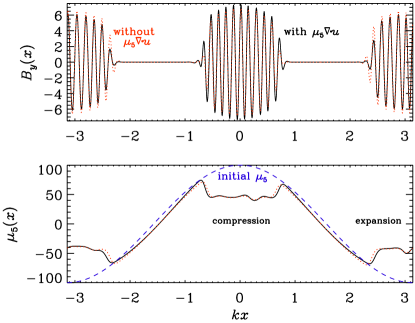
Figure 14.— Comparison of the profiles of $B_{y}(x)$ and ${\mu}_{5}(x)$ for $k=1$, ${\mu}_{50}=100$, $\lambda=100$, $\eta=10^{-3}$, and $u_{0}=10^{-2}$ with (black) and without (red) the ${\mu}_{5}\mbox{\boldmath$\nabla$}{}\cdot\bm{u}$ term included. The initial profile of ${\mu}_{5}$ is also shown (blue dashed).

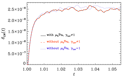
Figure 15.— Comparison of ${\cal E}_{\rm GW}(t)$ for the cases where $\gamma_{\rm Lor}\neq 1$ and the ${\mu}_{5}\mbox{\boldmath$\nabla$}{}\cdot\bm{u}$ term is included (black solid) and where it is omitted (red dashed) with a case where $\gamma_{\rm Lor}=1$ and the ${\mu}_{5}\mbox{\boldmath$\nabla$}{}\cdot\bm{u}$ term is included (blue dotted).

When conservation of the total chirality is invoked by including the ${\mu}_{5}\mbox{\boldmath$\nabla$}{}\cdot\bm{u}$ term, there is a small enhancement of $B_{y}$ around $kx=\pm 0.7$ and a small decrease at $\pm 2.3$. This is caused by compression at $kx=0$ and expansion at $kx=\pm\pi$. In this example, when the ${\mu}_{5}\mbox{\boldmath$\nabla$}{}\cdot\bm{u}$ term is absent, the total chirality becomes negative and reaches about 6% of its initial rms value. Finally, we show in Figure 15 the evolution of ${\cal E}_{\rm GW}(t)$ for Run D8, where the magnetic field is one of the largest and the effect of the ${\mu}_{5}\mbox{\boldmath$\nabla$}{}\cdot\bm{u}$ term is expected to be strong. We compare the case where $\gamma_{\rm Lor}\neq 1$ and the ${\mu}_{5}\mbox{\boldmath$\nabla$}{}\cdot\bm{u}$ term is included with a case where it is omitted, and a case where $\gamma_{\rm Lor}=1$ and the ${\mu}_{5}\mbox{\boldmath$\nabla$}{}\cdot\bm{u}$ term is included. The effect of the latter is here extremely small. We also see that the inclusion of the $\gamma_{\rm Lor}$ term affects the detailed time evolution of ${\cal E}_{\rm GW}(t)$, but not the final overall saturation level.

References

- Aharonian et al. (2006) Aharonian, F., Akhperjanian, A. G., Bazer-Bachi, A. R., et al. 2006, Natur, 440, 1018
- Anand et al. (2019) Anand, S., Bhatt, J. R., Pandey, A. K., & Kumar, A. 2019, Eur. Phys. J. C, 79, 119
- Arnold et al. (2000) Arnold, P., Moore, G. D., & Yaffe, L. G. 2000, JHEP, 11, 001
- Boyarsky et al. (2021) Boyarsky, A., Cheianov, V., Ruchayskiy, O., & Sobol, O. 2021, PhRvD, 103, 013003
- Boyarsky et al. (2012) Boyarsky, A., Fröhlich, J., & Ruchayskiy, O. 2012, Phys. Rev. Lett., 108, 031301
- Boyarsky et al. (2015) Boyarsky, A., Fröhlich, J., & Ruchayskiy, O. 2015, PhRvD, 92, 043004
- Brandenburg (2018) Brandenburg, A., on behalf of the Pencil Code Collaboration, 2018, Pencil Code, v2018.12.16, Zenodo, DOI:10.5281/zenodo.2315093
- Brandenburg & Boldyrev (2020) Brandenburg, A., & Boldyrev, S. 2020, ApJ, 892, 80
- Pencil Code Collaboration (2021) Pencil Code Collaboration: Brandenburg, A., Johansen, A., Bourdin, P. A., Dobler, W., Lyra, W., Rheinhardt, M., Bingert, S., Haugen, N. E. L., Mee, A., Gent, F., Babkovskaia, N., Yang, C.-C., Heinemann, T., Dintrans, B., Mitra, D., Candelaresi, S., Warnecke, J., Käpylä, P. J., Schreiber, A., Chatterjee, P., Käpylä, M. J., Li, X.-Y., Krüger, J., Aarnes, J. R., Sarson, G. R., Oishi, J. S., Schober, J., Plasson, R., Sandin, C., Karchniwy, E., Rodrigues, L. F. S., Hubbard, A., Guerrero, G., Snodin, A., Losada, I. R., Pekkilä, J., & Qian, C. 2021, Journal of Open Source Software, 6, 2807 arXiv:2009.08231, doi: 10.21105/joss.02807
- Brandenburg & Kahniashvili (2017) Brandenburg, A., & Kahniashvili, T. 2017, Phys. Rev. Lett., 118, 055102
- Brandenburg et al. (1996) Brandenburg, A., Enqvist, K., & Olesen, P. 1996, PhRvD, 54, 1291
- Brandenburg et al. (2017a) Brandenburg, A., Kahniashvili, T., Mandal, S., Roper Pol, A., Tevzadze, A. G., & Vachaspati, T. 2017a, PhRvD, 96, 123528
- Brandenburg et al. (2017b) Brandenburg, A., Schober, J., Rogachevskii, I., Kahniashvili, T., Boyarsky, A., Fröhlich, J., Ruchayskiy, O., & Kleeorin, N. 2017b, ApJ, 845, L21
- Caprini et al. (2019) Caprini, C., Chala, M., Dorsch, G. C., Hindmarsh, M., Huber, S. J., Konstandin, T., Kozaczuk, J., Nardini, G., No J. M., & Rummukainen, K. 2019, JCAP, 03, 024
- Deryagin et al. (1987) Deryagin, D. V., Grigoriev, D. Y., Rubakov, V. A., & Sazhin, M. V. 1987, MNRAS, 229, 357
- Díaz-Gil (2008a) Díaz-Gil, A., García-Bellido, J., García Pérez, M., & González-Arroyo, A. 2008a, Phys. Rev. Lett., 100, 241301
- Díaz-Gil (2008b) Díaz-Gil, A., García-Bellido, J., García Pérez, M., & González-Arroyo, A. 2008b, J. High Energy Phys., 2008, 07043
- Durrer & Caprini (2003) Durrer, R., & Caprini, C. 2003, JCAP, 0311, 010
- Durrer & Neronov (2013) Durrer, R., & Neronov, A. 2013, A&A Rev., 21, 62
- Gogoberidze et al. (2007) Gogoberidze, G., Kahniashvili, T., & Kosowsky, A. 2007, PhRvD, 76, 083002
- Grasso & Rubinstein (2001) Grasso, D., & Rubinstein, H. R. 2001, Phys. Rev., 348, 163
- Hindmarsh et al. (2015) Hindmarsh, M., Huber, S. J., Rummukainen, K., & Weir, D. J. 2015, PhRvD, 92, 123009
- Joyce & Shaposhnikov (1997) Joyce, M., & Shaposhnikov, M. 1997, Phys. Rev. Lett., 79, 1193
- Kahniashvili et al. (2021) Kahniashvili, T., Brandenburg, A., Gogoberidze, G., Mandal, S., & Roper Pol, A. 2020, PhRvR, in press, arXiv:2011.05556
- Kahniashvili et al. (2013) Kahniashvili, T., Tevzadze, A. G., Brandenburg, A., & Neronov, A. 2013, PhRvD, 87, 083007
- Kosowsky et al. (2002) Kosowsky, A., Mack, A., & Kahniashvili, T. 2002, PhRvD, 66, 024030
- Okano & Fujita (2021) Okano, S., & Fujita, T. 2021, JCAP, 03, 026
- Neronov & Vovk (2010) Neronov, A., & Vovk, I. 2010, Science, 328, 73
- Neronov et al. (2021) Neronov, A., Roper Pol, A., Caprini, C., & Semikoz, D. 2021, PhRvD, 103, L041302
- Rogachevskii et al. (2017) Rogachevskii, I., Ruchayskiy, O., Boyarsky, A., Fröhlich, J., Kleeorin, N., Brandenburg, A., & Schober, J. 2017, ApJ, 846, 153
- Roper Pol et al. (2020a) Roper Pol, A., Brandenburg, A., Kahniashvili, T., Kosowsky, A., & Mandal, S. 2020a, Geophys. Astrophys. Fluid Dyn., 114, 130
- Roper Pol et al. (2020b) Roper Pol, A., Mandal, S., Brandenburg, A., Kahniashvili, T., & Kosowsky, A. 2020b, PhRvD, 102, 083512
- Sharma et al. (2020) Sharma, R., Subramanian, K., & Seshadri, T. R. 2020, PhRvD, 101, 103526
- Schober et al. (2018) Schober, J., Rogachevskii, I., Brandenburg, A., Boyarsky, A., Fröhlich, J., Ruchayskiy, O., & Kleeorin, N. 2018, ApJ, 858, 124
- Schober et al. (2020) Schober, J., Brandenburg, A., & Rogachevskii, I. 2020, Geophys. Astrophys. Fluid Dyn., 114, 106
- Taylor et al. (2011) Taylor, A. M., Vovk, I., & Neronov, A. 2011, A&A, 529, A144
- Vilenkin (1980) Vilenkin, A. 1980, PhRvD, 22, 3080