Polarization of gravitational waves from helical MHD turbulent sources

Abstract

We use direct numerical simulations of decaying primordial hydromagnetic turbulence with helicity to compute the resulting gravitational wave (GW) production and its degree of circular polarization. The turbulence is sourced by magnetic fields that are either initially present or driven by an electromotive force applied for a short duration, given as a fraction of one Hubble time. In both types of simulations, we find a clear dependence of the polarization of the resulting GWs on the fractional helicity of the turbulent source. We find a low frequency tail below the spectral peak shallower than the $f^{3}$ scaling expected at super-horizon scales, in agreement with similar recent numerical simulations. This type of spectrum facilitates its observational detection with the planned Laser Interferometer Space Antenna (LISA). We show that driven magnetic fields produce GWs more efficiently than magnetic fields that are initially present, leading to larger spectral amplitudes, and to modifications of the spectral shape. In particular, we observe a sharp drop of GW energy above the spectral peak that is in agreement with the previously obtained results. The helicity does not have a huge impact on the maximum spectral amplitude in any of the two types of turbulence considered. However, the GW spectrum at wave numbers away from the peak becomes smaller for larger values of the magnetic fractional helicity. Such variations of the spectrum are most noticeable when magnetic fields are driven. The degree of circular polarization approaches zero at frequencies below the peak, and reaches its maximum at the peak. At higher frequencies, it stays finite if the magnetic field is initially present, and it approaches zero if it is driven. We predict that the spectral peak of the GW signal can be detected by LISA if the turbulent energy density is at least $\sim\!3\%$ of the radiation energy density, and the characteristic scale is a hundredth of the horizon at the electroweak scale. We show that the resulting GW polarization is unlikely to be detectable by the anisotropies induced by our proper motion in the dipole response function of LISA. Such signals can, however, be detectable by cross-correlating data from the LISA–Taiji network for turbulent energy densities of $\sim\!5\%$, and fractional helicity of 0.5 to 1. Second-generation space-based GW detectors, such as the Big Bang Observer (BBO) and the DECi-hertz Interferometer Gravitational wave Observatory (DECIGO), would allow for the detection of a larger range of the GW spectrum and smaller amplitudes of the magnetic field.

1 Introduction

Primordial turbulent magnetic fields produced and/or present during phase transitions in the early universe generate a stochastic background of gravitational waves (GWs) [1]; see refs. [3, 2] for reviews. Assuming the standard energy scales of cosmological phase transitions ($T_{*}\sim 100\,{\rm GeV}$ for the electroweak, and $T_{*}\sim 100\,{\rm MeV}$ for the QCD phase transition), and accounting that the characteristic scale of the magnetic field at the moment of its generation is limited by the Hubble horizon scale and it is taken to be a fraction of it (this fraction is determined by the size of the magnetic field eddies, which is related to the phase transition bubble size in the case of a first order phase transition, and/or by the energy containing wave number $k_{*}$ of the turbulent motions in other scenarios), the characteristic typical frequencies of the GW spectrum range from nHz to Hz [4, 5, 6]. Future space-based GW detectors such as the Laser Interferometer Space Antenna (LISA) [7], planned to be launched in 2034, as well as TianQin [8] and Taiji [9], will be sensitive to GWs in frequencies ranging from 10 $\mu$Hz to a few Hz, with a peak sensitivity around 1 mHz (LISA and Taiji) and a few mHz (TianQin). Actually, this is a typical Hubble frequency range for the electroweak phase transition (EWPT) if occurring around 10 TeV. In this range of frequencies, we expect magnetic fields and turbulence yielding GW signals generated at the EWPT; see ref. [10] for pioneering work and refs. [11, 12, 13] for subsequent studies. Importantly, the main parameters of the turbulence (and, correspondingly, the characteristics of the phase transitions) are imprinted on the GW signal shape, amplitude, and polarization [14, 15].

Additional sources from a first-order phase transition producing GW radiation in this range of frequencies include the collision of scalar field shells, sound waves induced into the surrounding plasma, and subsequent turbulent motions; see ref. [16] for a pioneering work and refs. [17, 18] for recent reviews, and references therein. In addition, the next generation of space-based GW detectors is planned to improve the sensitivity to GW signals and to cover the range from mHz to 10 Hz (which lies in between the sensitive frequencies of space-based GW detectors such as LISA and ground-based GW detectors such as the LIGO-Virgo-Kagra network), e.g., the DECi-hertz Interferometer Gravitational wave Observatory (DECIGO) [19], and the Big Bang Observer (BBO) [20, 21]. In the lower regime of frequencies, measuring the time of arrival by a pulsar timing array (PTA) allows one to detect GW signals in the range from $10^{-9}$–$10^{-7}$ Hz, which corresponds to the GW signals generated during a phase transition with typical energy scales from a few MeV to one GeV, such as the QCD phase transition, with a typical scale of about $100\,{\rm MeV}$; see refs. [22, 4, 23, 24] and ref. [25] for a review, and references therein. This frequency range is also typical for the blue tilted GW spectrum originated from the inflationary epoch; see ref. [25] for a review and references therein. Even smaller frequencies can be probed by the indirect detection of $B$-modes in the cosmic microwave background (CMB) polarization [26, 27], which, along with temperature and $E$-mode polarization anisotropies, can be produced by inflation-generated GW signals [29, 28]. The treatment of the early-universe generated GW energy density spectrum allows one to constrain different scenarios by PTA measurements, laser interferometer experiments, and big bang nucleosynthesis (BBN) bounds [30]. In addition, large surveys of stars like Gaia [31] or the proposed Theia [32] have been recently proposed to detect GWs in the range of frequencies around the QCD scale [33, 34].

There is various kind of evidence for magnetic fields in the largest scales of the universe [3], which can have their origin in astrophysical or cosmological seed fields. In particular, primordial magnetic fields are motivated by the lower limits on the strength of extragalactic magnetic fields inferred by observations of blazar spectra by the Fermi Gamma-ray Observatory; see ref. [35] for a pioneering work and ref. [36] for a recent review, and references therein. Such fields are strongly coupled to the primordial plasma due to the high conductivity of the early universe, inevitably leading to magnetohydrodynamic (MHD) turbulence; see refs. [37, 38] for pioneering work and ref. [39] for a recent study. In addition, any primordial turbulent process during the early universe can also reinforce the magnetic field; see ref. [40] for a discussion of the dynamo mechanism in decaying turbulence.

The cosmological evolution of the magnetic field strongly depends on helicity [41, 42], yielding magnetic fields with larger coherent scales and favoring the constraints from Fermi observations (see ref. [36] for a review and references therein). Parity-violating processes at the EWPT leading to the generation of helical magnetic fields have been proposed. Some examples are: via sphaleron decay (see ref. [43] for a non-helical case and ref. [44] for a helical case), due to the generation of Chern-Simons number through $B+L$ anomalies [45], and due to inhomogeneities in the Higgs field in low-scale electroweak hybrid inflation [46, 47, 48, 49, 50, 51]. The presence of a cosmic axion field also leads to the generation of helicity in existing primordial magnetic fields [52, 53]. Magnetic fields can also be produced during inflation; see refs. [54, 43, 56, 55, 57, 58] for pioneering work and the reviews [59, 60, 36], and references therein. Some mechanisms have been proposed to add helicity into the inflationary magnetogenesis models; see ref. [61] for pioneering work and refs. [60, 36] for reviews, and references therein.

As expected, primordial helical magnetic fields produce circularly polarized GWs [62, 63, 65, 64]. In particular, the detection of circularly polarized GWs, proposed in refs. [66, 67], will shed light on phenomena of fundamental symmetry breaking in the early universe, such as parity violation, and potentially can serve as an explanation of the lepto- and baryogenesis asymmetry problem; see refs. [68, 69, 70, 71, 72] for pioneering work, ref. [73] for a review, and refs. [74, 75, 76] for recent work. The dependence of the degree of polarization of GWs on the helicity of the source has been a matter of uncertainty owing to the approximations made in the analytical calculations available to date. In particular, previous works (see refs. [62, 63]) showed that the maximum circular polarization depends on the relation between the magnetic energy and the magnetic helicity spectra. Assuming Kolmogorov-type turbulence, with spectral index of $-5/3$ for the magnetic energy density and $-8/3$ for the helicity, following phenomenological modeling of ref. [77], the circular polarization of GWs would be at most about 80% for a maximally helical magnetic field [62, 63]. Following refs. [62, 63], we call this helical Kolmogorov (HK) turbulence. It can actually reach nearly 100% in the case when the spectral indices are equal, which we call a Moiseev-Chkhetiani type spectrum; see ref. [78], or helical transfer (HT) turbulence, following refs. [62, 63]. On small scales, the HT turbulence is dominated by helicity dissipation, and hence, the transfer of helicity is effective. Thus, the resulting degree of polarization stays constant at large wave numbers, and approximately equal to the fractional magnetic helicity. On the other hand, the HK turbulence is dominated by energy dissipation, such that the polarization decays to zero due to the vanishing helicity [62]. In both cases, the spectral peak of the polarization spectrum is at the same scale as the GW spectral peak, which is at a wave number approximately twice the wave number of the magnetic spectral peak. For low values of the fractional magnetic helicity, the maximum degree of polarization also diminishes. More recently, the two types of spectra have been studied to model the turbulence produced in a first-order EWPT in ref. [64], in the context of detection prospects with LISA by using the dipole modulation induced by the proper motion of the solar system, as proposed in refs. [66, 67], and recently applied to LISA in ref. [79]. The potential detection of polarization can be improved by cross-correlating two space-based GW detectors as, for example, LISA and Taiji [80, 81]. We show that the circular degree of polarization computed from direct numerical simulations follows the HT turbulence model of previous analytical works if the magnetic field is assumed to be present at the initial time of generation. This scenario neglects the production of GWs that occurs while the magnetic field is generated by any of the described magnetogenesis mechanisms or via MHD dynamo. When we consider a magnetic field that is initially zero and it builds up during the simulation, following ref. [82], both the HK and the HT models of turbulence fail to predict the spectrum of the degree of circular polarization, and numerical simulations are required [65].

Recently, in refs. [83, 82], the authors have described the implementation of a GW solver into the Pencil Code [84] and have presented direct numerical simulations for modeling development and dynamics of primordial hydrodynamic and hydromagnetic turbulence from phase transitions, and subsequent generation of a stochastic GW background, also computed numerically. Their simulations included fully helical sources, but the estimation of the GW polarization degree spectrum, as well as the polarization detection prospects, were not the focus of their studies. We present here two types of simulations, similar to the two types of hydromagnetic simulations presented in ref. [82]: one where a primordial magnetic field is assumed to be given as the initial condition and one where a magnetic field is generated by an electromotive force $\mbox{\boldmath${\cal F}$}{}(\mathchoice{\mbox{\boldmath$\displaystyle x$}}{\mbox{\boldmath$\textstyle x$}}{\mbox{\boldmath$\scriptstyle x$}}{\mbox{\boldmath$\scriptscriptstyle x$}}{},t)$ that depends on time $t$ and position $\textstyle x$. In particular, regarding the first type, we study the cases with an initial stochastic magnetic field with different values of the fractional helicity, from non-helical up to the fully helical case. In ref. [65], the degree of circular polarization for kinetically and magnetically forced turbulence was presented, which is similar to our second type of simulations. We complement their analysis in the present work by studying the variation of the polarization degree in the different scenarios of the magnetic field generation. Furthermore, we study cases where turbulence is driven for times significantly shorter than what was considered in ref. [65]. The driving is then applied during a short time interval (around a 10% of the Hubble time), and then switched off such that turbulence decays for later times. By using suitably scaled variables and conformal time, the governing equations describing the evolution of GWs and turbulent magnetic fields in an expanding universe in the radiation era can be brought into a form that is best suited for numerical simulations [83]. We explore the detectability of the generated GW signal and its polarization with planned space-based GW detectors.

We begin by summarizing our approach and the equations solved in section 2. We then present the magnetic and GW energy spectra obtained from the numerical simulations in section 3. In particular, the degree of circular polarization is shown in section 3.3 and compared with previous analytical models in section 3.4. We explore the potential detectability of the GW background amplitude and polarization by space-based GW detectors and, in particular, by combining LISA and Taiji, in section 4, and we conclude in section 5.

Throughout this work, electromagnetic quantities are expressed in Lorentz–Heaviside units where the vacuum permeability is unity. Einstein index notation is used so summation is assumed over repeated indices. Latin indices $i$ and $j$ refer to spatial coordinates 1 to 3. The Kronecker delta is indicated by $\delta_{ij}$, the Levi-Civita tensor by $\varepsilon_{ijk}$, the Dirac delta function by $\delta(x)$, and the Heaviside step function by $\Theta(x)$.

2 The model

2.1 Gravitational signal from MHD turbulence

We perform direct numerical simulations of the MHD turbulence starting at the time of generation, which belongs to the radiation-dominated era and can be appropriately scaled to, e.g., the EWPT. At every time step of the MHD simulation, we compute the contributions from velocity and magnetic fields to the stress tensor $T_{ij}$. Then, we solve the GW equation to compute the strains $h_{ij}$, sourced by the traceless and transverse projection of the stress tensor. The details of the numerical setup and application to the electroweak scale are described in refs. [83, 82].

We use the linear polarization modes $+$ and $\times$ to describe the two gauge-independent components of the tensor mode perturbations, such that $\tilde{h}_{ij}(\mathchoice{\mbox{\boldmath$\displaystyle k$}}{\mbox{\boldmath$\textstyle k$}}{\mbox{\boldmath$\scriptstyle k$}}{\mbox{\boldmath$\scriptscriptstyle k$}}{})=\tilde{h}_{+}(\mathchoice{\mbox{\boldmath$\displaystyle k$}}{\mbox{\boldmath$\textstyle k$}}{\mbox{\boldmath$\scriptstyle k$}}{\mbox{\boldmath$\scriptscriptstyle k$}}{})e_{ij}^{+}(\hat{\mathchoice{\mbox{\boldmath$\displaystyle k$}}{\mbox{\boldmath$\textstyle k$}}{\mbox{\boldmath$\scriptstyle k$}}{\mbox{\boldmath$\scriptscriptstyle k$}}{}})+\tilde{h}_{\times}(\mathchoice{\mbox{\boldmath$\displaystyle k$}}{\mbox{\boldmath$\textstyle k$}}{\mbox{\boldmath$\scriptstyle k$}}{\mbox{\boldmath$\scriptscriptstyle k$}}{})e_{ij}^{\times}(\hat{\mathchoice{\mbox{\boldmath$\displaystyle k$}}{\mbox{\boldmath$\textstyle k$}}{\mbox{\boldmath$\scriptstyle k$}}{\mbox{\boldmath$\scriptscriptstyle k$}}{}})$ [85], where the tilde indicates that this decomposition is performed in Fourier space, and $\hat{\mathchoice{\mbox{\boldmath$\displaystyle k$}}{\mbox{\boldmath$\textstyle k$}}{\mbox{\boldmath$\scriptstyle k$}}{\mbox{\boldmath$\scriptscriptstyle k$}}}{}=\mathchoice{\mbox{\boldmath$\displaystyle k$}}{\mbox{\boldmath$\textstyle k$}}{\mbox{\boldmath$\scriptstyle k$}}{\mbox{\boldmath$\scriptscriptstyle k$}}{}/|\mathchoice{\mbox{\boldmath$\displaystyle k$}}{\mbox{\boldmath$\textstyle k$}}{\mbox{\boldmath$\scriptstyle k$}}{\mbox{\boldmath$\scriptscriptstyle k$}}{}|$. The linear polarization basis tensors are

$$e_{ij}^{+}(\hat{\mathchoice{\mbox{\boldmath$\displaystyle k$}}{\mbox{\boldmath$\textstyle k$}}{\mbox{\boldmath$\scriptstyle k$}}{\mbox{\boldmath$\scriptscriptstyle k$}}}{})=e_{i}^{1}e_{j}^{1}-e_{i}^{2}e_{j}^{2},\quad e_{ij}^{\times}(\hat{\mathchoice{\mbox{\boldmath$\displaystyle k$}}{\mbox{\boldmath$\textstyle k$}}{\mbox{\boldmath$\scriptstyle k$}}{\mbox{\boldmath$\scriptscriptstyle k$}}}{})=e_{i}^{1}e_{j}^{2}+e_{i}^{2}e_{j}^{1},$$ (2.1)

where $\mathchoice{\mbox{\boldmath$\displaystyle e$}}{\mbox{\boldmath$\textstyle e$}}{\mbox{\boldmath$\scriptstyle e$}}{\mbox{\boldmath$\scriptscriptstyle e$}}{}^{1}$ and $\mathchoice{\mbox{\boldmath$\displaystyle e$}}{\mbox{\boldmath$\textstyle e$}}{\mbox{\boldmath$\scriptstyle e$}}{\mbox{\boldmath$\scriptscriptstyle e$}}{}^{2}$ form a basis with the unit vector $\hat{\mathchoice{\mbox{\boldmath$\displaystyle k$}}{\mbox{\boldmath$\textstyle k$}}{\mbox{\boldmath$\scriptstyle k$}}{\mbox{\boldmath$\scriptscriptstyle k$}}}{}$ [86]. We solve the non-dimensional GW equation in the radiation era for the scaled strains $\tilde{h}_{+,\times}(\mathchoice{\mbox{\boldmath$\displaystyle k$}}{\mbox{\boldmath$\textstyle k$}}{\mbox{\boldmath$\scriptstyle k$}}{\mbox{\boldmath$\scriptscriptstyle k$}}{},t)$ [1], using conformal time, normalized to unity at the initial time of magnetic field generation $t_{\ast}$, and comoving wave vector, normalized by $1/(ct_{\ast})$, as described in refs. [83, 82],

$$\left(\partial^{2}_{t}+\mathchoice{\mbox{\boldmath$\displaystyle k$}}{\mbox{\boldmath$\textstyle k$}}{\mbox{\boldmath$\scriptstyle k$}}{\mbox{\boldmath$\scriptscriptstyle k$}}{}^{2}\right)\tilde{h}_{+,\times}(\mathchoice{\mbox{\boldmath$\displaystyle k$}}{\mbox{\boldmath$\textstyle k$}}{\mbox{\boldmath$\scriptstyle k$}}{\mbox{\boldmath$\scriptscriptstyle k$}}{},t)\,=\,{6\over t}\tilde{T}_{+,\times}^{\rm TT}(\mathchoice{\mbox{\boldmath$\displaystyle k$}}{\mbox{\boldmath$\textstyle k$}}{\mbox{\boldmath$\scriptstyle k$}}{\mbox{\boldmath$\scriptscriptstyle k$}}{},t),$$ (2.2)

where $\tilde{T}_{+,\times}^{\rm TT}(\mathchoice{\mbox{\boldmath$\displaystyle k$}}{\mbox{\boldmath$\textstyle k$}}{\mbox{\boldmath$\scriptstyle k$}}{\mbox{\boldmath$\scriptscriptstyle k$}}{},t)$ is the comoving stress tensor, projected into the traceless and transverse (TT) gauge, described by the linear polarization modes $+$ and $\times$, and normalized by the energy density at $t_{\ast}$. The scaled strains are tensor mode perturbations over the Friedmann-Lemaître-Robertson-Walker metric tensor, such that the line element is ${\rm d}{}s^{2}=a^{2}(-{\rm d}{}t^{2}+[\delta_{ij}+h_{ij}/a]\,{\rm d}{}x_{i}\,{\rm d}{}x_{j})$. During the radiation-dominated epoch, the equation of state is $p={\textstyle{1\over 3}}\rho$, where $\rho$ is the energy density and $p$ the pressure. This leads to a linear evolution of the scale factor $a$ with $t$, and allows one to get rid of the damping term [87], which should be included otherwise in equation (2.2)., one should substitute $t$ by $a$ in the denominator of the sourcing term of equation (2.2). The stress is composed of magnetic and kinetic contributions and computed in physical space as

$$T_{ij}(\mathchoice{\mbox{\boldmath$\displaystyle x$}}{\mbox{\boldmath$\textstyle x$}}{\mbox{\boldmath$\scriptstyle x$}}{\mbox{\boldmath$\scriptscriptstyle x$}}{})=\frac{4}{3}\frac{\rho u_{i}u_{j}}{1-\mathchoice{\mbox{\boldmath$\displaystyle u$}}{\mbox{\boldmath$\textstyle u$}}{\mbox{\boldmath$\scriptstyle u$}}{\mbox{\boldmath$\scriptscriptstyle u$}}{}^{2}}-B_{i}B_{j}+\left(\frac{\rho}{3}+\frac{\mathchoice{\mbox{\boldmath$\displaystyle B$}}{\mbox{\boldmath$\textstyle B$}}{\mbox{\boldmath$\scriptstyle B$}}{\mbox{\boldmath$\scriptscriptstyle B$}}{}^{2}}{2}\right)\delta_{ij},$$ (2.3)

where $\textstyle u$ is the plasma velocity and $\textstyle B$ is the magnetic field. The total enthalpy is $w=p+\rho={\textstyle{4\over 3}}\rho$. Since $T_{ij}$ refers to comoving and normalized stress tensor, the MHD fields ($\rho$, $\textstyle u$, and $\textstyle B$) are accordingly normalized and comoving.

The non-dimensional and comoving MHD equations for an ultrarelativistic gas in a flat expanding universe in the radiation-dominated era after the EWPT are given by [38]

$${\partial\ln\rho\over\partial t} = -\frac{4}{3}\left(\mathchoice{\mbox{\boldmath$\displaystyle\nabla$}}{\mbox{\boldmath$\textstyle\nabla$}}{\mbox{\boldmath$\scriptstyle\nabla$}}{\mbox{\boldmath$\scriptscriptstyle\nabla$}}{}\cdot\mathchoice{\mbox{\boldmath$\displaystyle u$}}{\mbox{\boldmath$\textstyle u$}}{\mbox{\boldmath$\scriptstyle u$}}{\mbox{\boldmath$\scriptscriptstyle u$}}{}+\mathchoice{\mbox{\boldmath$\displaystyle u$}}{\mbox{\boldmath$\textstyle u$}}{\mbox{\boldmath$\scriptstyle u$}}{\mbox{\boldmath$\scriptscriptstyle u$}}{}\cdot\mathchoice{\mbox{\boldmath$\displaystyle\nabla$}}{\mbox{\boldmath$\textstyle\nabla$}}{\mbox{\boldmath$\scriptstyle\nabla$}}{\mbox{\boldmath$\scriptscriptstyle\nabla$}}{}\ln\rho\right)+{1\over\rho}\left[\mathchoice{\mbox{\boldmath$\displaystyle u$}}{\mbox{\boldmath$\textstyle u$}}{\mbox{\boldmath$\scriptstyle u$}}{\mbox{\boldmath$\scriptscriptstyle u$}}{}\cdot(\mathchoice{\mbox{\boldmath$\displaystyle J$}}{\mbox{\boldmath$\textstyle J$}}{\mbox{\boldmath$\scriptstyle J$}}{\mbox{\boldmath$\scriptscriptstyle J$}}{}\times\mathchoice{\mbox{\boldmath$\displaystyle B$}}{\mbox{\boldmath$\textstyle B$}}{\mbox{\boldmath$\scriptstyle B$}}{\mbox{\boldmath$\scriptscriptstyle B$}}{})+\eta\mathchoice{\mbox{\boldmath$\displaystyle J$}}{\mbox{\boldmath$\textstyle J$}}{\mbox{\boldmath$\scriptstyle J$}}{\mbox{\boldmath$\scriptscriptstyle J$}}{}^{2}\right],$$ (2.4)

$${\partial\mathchoice{\mbox{\boldmath$\displaystyle u$}}{\mbox{\boldmath$\textstyle u$}}{\mbox{\boldmath$\scriptstyle u$}}{\mbox{\boldmath$\scriptscriptstyle u$}}{}\over\partial t} = -\mathchoice{\mbox{\boldmath$\displaystyle u$}}{\mbox{\boldmath$\textstyle u$}}{\mbox{\boldmath$\scriptstyle u$}}{\mbox{\boldmath$\scriptscriptstyle u$}}{}\cdot\mathchoice{\mbox{\boldmath$\displaystyle\nabla$}}{\mbox{\boldmath$\textstyle\nabla$}}{\mbox{\boldmath$\scriptstyle\nabla$}}{\mbox{\boldmath$\scriptscriptstyle\nabla$}}{}\mathchoice{\mbox{\boldmath$\displaystyle u$}}{\mbox{\boldmath$\textstyle u$}}{\mbox{\boldmath$\scriptstyle u$}}{\mbox{\boldmath$\scriptscriptstyle u$}}{}+{\mathchoice{\mbox{\boldmath$\displaystyle u$}}{\mbox{\boldmath$\textstyle u$}}{\mbox{\boldmath$\scriptstyle u$}}{\mbox{\boldmath$\scriptscriptstyle u$}}{}\over 3}\left(\mathchoice{\mbox{\boldmath$\displaystyle\nabla$}}{\mbox{\boldmath$\textstyle\nabla$}}{\mbox{\boldmath$\scriptstyle\nabla$}}{\mbox{\boldmath$\scriptscriptstyle\nabla$}}{}\cdot\mathchoice{\mbox{\boldmath$\displaystyle u$}}{\mbox{\boldmath$\textstyle u$}}{\mbox{\boldmath$\scriptstyle u$}}{\mbox{\boldmath$\scriptscriptstyle u$}}{}+\mathchoice{\mbox{\boldmath$\displaystyle u$}}{\mbox{\boldmath$\textstyle u$}}{\mbox{\boldmath$\scriptstyle u$}}{\mbox{\boldmath$\scriptscriptstyle u$}}{}\cdot\mathchoice{\mbox{\boldmath$\displaystyle\nabla$}}{\mbox{\boldmath$\textstyle\nabla$}}{\mbox{\boldmath$\scriptstyle\nabla$}}{\mbox{\boldmath$\scriptscriptstyle\nabla$}}{}\ln\rho\right)+{2\over\rho}\mathchoice{\mbox{\boldmath$\displaystyle\nabla$}}{\mbox{\boldmath$\textstyle\nabla$}}{\mbox{\boldmath$\scriptstyle\nabla$}}{\mbox{\boldmath$\scriptscriptstyle\nabla$}}{}\cdot\left(\rho\nu\bm{\mathsf{S}}\right)$$ (2.5)

$$-{1\over 4}\mathchoice{\mbox{\boldmath$\displaystyle\nabla$}}{\mbox{\boldmath$\textstyle\nabla$}}{\mbox{\boldmath$\scriptstyle\nabla$}}{\mbox{\boldmath$\scriptscriptstyle\nabla$}}{}\ln\rho-{\mathchoice{\mbox{\boldmath$\displaystyle u$}}{\mbox{\boldmath$\textstyle u$}}{\mbox{\boldmath$\scriptstyle u$}}{\mbox{\boldmath$\scriptscriptstyle u$}}{}\over\rho}\left[\mathchoice{\mbox{\boldmath$\displaystyle u$}}{\mbox{\boldmath$\textstyle u$}}{\mbox{\boldmath$\scriptstyle u$}}{\mbox{\boldmath$\scriptscriptstyle u$}}{}\cdot(\mathchoice{\mbox{\boldmath$\displaystyle J$}}{\mbox{\boldmath$\textstyle J$}}{\mbox{\boldmath$\scriptstyle J$}}{\mbox{\boldmath$\scriptscriptstyle J$}}{}\times\mathchoice{\mbox{\boldmath$\displaystyle B$}}{\mbox{\boldmath$\textstyle B$}}{\mbox{\boldmath$\scriptstyle B$}}{\mbox{\boldmath$\scriptscriptstyle B$}}{})+\eta\mathchoice{\mbox{\boldmath$\displaystyle J$}}{\mbox{\boldmath$\textstyle J$}}{\mbox{\boldmath$\scriptstyle J$}}{\mbox{\boldmath$\scriptscriptstyle J$}}{}^{2}\right]+{3\over 4\rho}\mathchoice{\mbox{\boldmath$\displaystyle J$}}{\mbox{\boldmath$\textstyle J$}}{\mbox{\boldmath$\scriptstyle J$}}{\mbox{\boldmath$\scriptscriptstyle J$}}{}\times\mathchoice{\mbox{\boldmath$\displaystyle B$}}{\mbox{\boldmath$\textstyle B$}}{\mbox{\boldmath$\scriptstyle B$}}{\mbox{\boldmath$\scriptscriptstyle B$}}{},$$

$${\partial\mathchoice{\mbox{\boldmath$\displaystyle B$}}{\mbox{\boldmath$\textstyle B$}}{\mbox{\boldmath$\scriptstyle B$}}{\mbox{\boldmath$\scriptscriptstyle B$}}{}\over\partial t} = \mathchoice{\mbox{\boldmath$\displaystyle\nabla$}}{\mbox{\boldmath$\textstyle\nabla$}}{\mbox{\boldmath$\scriptstyle\nabla$}}{\mbox{\boldmath$\scriptscriptstyle\nabla$}}{}\times(\mathchoice{\mbox{\boldmath$\displaystyle u$}}{\mbox{\boldmath$\textstyle u$}}{\mbox{\boldmath$\scriptstyle u$}}{\mbox{\boldmath$\scriptscriptstyle u$}}{}\times\mathchoice{\mbox{\boldmath$\displaystyle B$}}{\mbox{\boldmath$\textstyle B$}}{\mbox{\boldmath$\scriptstyle B$}}{\mbox{\boldmath$\scriptscriptstyle B$}}{}-\eta\mathchoice{\mbox{\boldmath$\displaystyle J$}}{\mbox{\boldmath$\textstyle J$}}{\mbox{\boldmath$\scriptstyle J$}}{\mbox{\boldmath$\scriptscriptstyle J$}}{}+\mbox{\boldmath${\cal F}$}{}),\quad\mathchoice{\mbox{\boldmath$\displaystyle J$}}{\mbox{\boldmath$\textstyle J$}}{\mbox{\boldmath$\scriptstyle J$}}{\mbox{\boldmath$\scriptscriptstyle J$}}{}=\mathchoice{\mbox{\boldmath$\displaystyle\nabla$}}{\mbox{\boldmath$\textstyle\nabla$}}{\mbox{\boldmath$\scriptstyle\nabla$}}{\mbox{\boldmath$\scriptscriptstyle\nabla$}}{}\times\mathchoice{\mbox{\boldmath$\displaystyle B$}}{\mbox{\boldmath$\textstyle B$}}{\mbox{\boldmath$\scriptstyle B$}}{\mbox{\boldmath$\scriptscriptstyle B$}}{},$$ (2.6)

where ${\sf S}_{ij}={\textstyle{1\over 2}}(\partial_{j}u_{i}+\partial_{i}u_{j})-{\textstyle{1\over 3}}\delta_{ij}\mathchoice{\mbox{\boldmath$\displaystyle\nabla$}}{\mbox{\boldmath$\textstyle\nabla$}}{\mbox{\boldmath$\scriptstyle\nabla$}}{\mbox{\boldmath$\scriptscriptstyle\nabla$}}{}\cdot\mathchoice{\mbox{\boldmath$\displaystyle u$}}{\mbox{\boldmath$\textstyle u$}}{\mbox{\boldmath$\scriptstyle u$}}{\mbox{\boldmath$\scriptscriptstyle u$}}{}$ are the components of the rate-of-strain tensor, $\textstyle J$ is the current density, $\nu$ is the kinematic viscosity, and $\eta$ is the magnetic diffusivity. The electromotive force ${\cal F}$ is used to model the generation of magnetic fields.

2.2 Magnetic fields present at the initial time

In the first type of runs, we consider the magnetic field to be present at the initial time of the simulation, so we set the electromotive force term ${\cal F}$ to be zero at all times. We generate a random three-dimensional vector field in Fourier space,

$$\tilde{B}_{i}({\mathchoice{\mbox{\boldmath$\displaystyle k$}}{\mbox{\boldmath$\textstyle k$}}{\mbox{\boldmath$\scriptstyle k$}}{\mbox{\boldmath$\scriptscriptstyle k$}}{}})=B_{0}\left(P_{ij}(\hat{\mathchoice{\mbox{\boldmath$\displaystyle k$}}{\mbox{\boldmath$\textstyle k$}}{\mbox{\boldmath$\scriptstyle k$}}{\mbox{\boldmath$\scriptscriptstyle k$}}}{})-i\sigma\epsilon_{ijl}\hat{k}_{l}\right)\tilde{g}_{j}({\hat{\mathchoice{\mbox{\boldmath$\displaystyle k$}}{\mbox{\boldmath$\textstyle k$}}{\mbox{\boldmath$\scriptstyle k$}}{\mbox{\boldmath$\scriptscriptstyle k$}}}{}})\,g_{0}(k),$$ (2.7)

where $B_{0}$ is the magnetic field amplitude, $\tilde{g}_{j}(\hat{\mathchoice{\mbox{\boldmath$\displaystyle k$}}{\mbox{\boldmath$\textstyle k$}}{\mbox{\boldmath$\scriptstyle k$}}{\mbox{\boldmath$\scriptscriptstyle k$}}}{})$ is the Fourier transform of a $\delta$-correlated vector field in three dimensions with Gaussian fluctuations, i.e., $g_{i}(\mathchoice{\mbox{\boldmath$\displaystyle x$}}{\mbox{\boldmath$\textstyle x$}}{\mbox{\boldmath$\scriptstyle x$}}{\mbox{\boldmath$\scriptscriptstyle x$}}{})g_{j}(\mathchoice{\mbox{\boldmath$\displaystyle x$}}{\mbox{\boldmath$\textstyle x$}}{\mbox{\boldmath$\scriptstyle x$}}{\mbox{\boldmath$\scriptscriptstyle x$}}{}^{\prime})=\delta_{ij}\delta^{3}(\mathchoice{\mbox{\boldmath$\displaystyle x$}}{\mbox{\boldmath$\textstyle x$}}{\mbox{\boldmath$\scriptstyle x$}}{\mbox{\boldmath$\scriptscriptstyle x$}}{}-\mathchoice{\mbox{\boldmath$\displaystyle x$}}{\mbox{\boldmath$\textstyle x$}}{\mbox{\boldmath$\scriptstyle x$}}{\mbox{\boldmath$\scriptscriptstyle x$}}{}^{\prime})$, $\sigma$ is a parameter that allows one to control the fractional magnetic helicity, $P_{ij}(\hat{\mathchoice{\mbox{\boldmath$\displaystyle k$}}{\mbox{\boldmath$\textstyle k$}}{\mbox{\boldmath$\scriptstyle k$}}{\mbox{\boldmath$\scriptscriptstyle k$}}}{})=\delta_{ij}-\hat{k}_{i}\hat{k}_{j}$ is the projection operator. The spectral shape is determined by $g_{0}(k)$ [39],

$$g_{0}(k)={k_{*}^{-3/2}(k/k_{*})^{\alpha/2-1}\over[1+(k/k_{*})^{2(\alpha-\beta)}]^{1/4}},$$ (2.8)

where $k_{*}$ sets the scale of the spectral peak, which is identified with the initial wave number of the energy-carrying eddies. The magnetic energy density is ${\cal E}_{\rm M}={\textstyle{1\over 2}}\langle\mathchoice{\mbox{\boldmath$\displaystyle B$}}{\mbox{\boldmath$\textstyle B$}}{\mbox{\boldmath$\scriptstyle B$}}{\mbox{\boldmath$\scriptscriptstyle B$}}{}^{2}\rangle$, such that its initial value is ${\cal E}_{\rm M}^{\rm max}={\textstyle{1\over 2}}B_{0}^{2}$. Due to the normalization used, this value corresponds to a fraction of the radiation energy density at the time of magnetic field generation, and since this case corresponds to decaying turbulence, ${\cal E}_{\rm M}^{\rm max}$ is the maximum value of the magnetic energy density. The magnetic spectrum $E_{\rm M}(k)$, computed such that ${\cal E}_{\rm M}=\int E_{\rm M}(k)\,{\rm d}{}k$, is proportional to $k^{2}g_{0}^{2}(k)$, with a spectral index $\alpha=4$ in the low wave number limit (subinertial range) for a Batchelor spectrum, and Kolmogorov-type spectral slope $\beta=-5/3$ in the high wave number range. Here, the $k_{*}^{-3/2}$ prefactor ensures that the resulting magnetic energy ${\cal E}_{\rm M}$ is independent of the value of $k_{*}$. The exponents $\zeta=2$ and $\zeta^{-2}=1/4$ in the denominator of equation (2.8) determine the transition smoothness from one slope to the other around the spectral peak. The initial fractional helicity of the magnetic field, ${\cal P}_{\rm M}=k_{*}\langle\mathchoice{\mbox{\boldmath$\displaystyle A$}}{\mbox{\boldmath$\textstyle A$}}{\mbox{\boldmath$\scriptstyle A$}}{\mbox{\boldmath$\scriptscriptstyle A$}}{}\cdot\mathchoice{\mbox{\boldmath$\displaystyle B$}}{\mbox{\boldmath$\textstyle B$}}{\mbox{\boldmath$\scriptstyle B$}}{\mbox{\boldmath$\scriptscriptstyle B$}}{}\rangle/\langle\mathchoice{\mbox{\boldmath$\displaystyle B$}}{\mbox{\boldmath$\textstyle B$}}{\mbox{\boldmath$\scriptstyle B$}}{\mbox{\boldmath$\scriptscriptstyle B$}}{}^{2}\rangle$, is given by $2\sigma/(1+\sigma^{2})$, being $\textstyle A$ the magnetic vector potential, such that $\mathchoice{\mbox{\boldmath$\displaystyle B$}}{\mbox{\boldmath$\textstyle B$}}{\mbox{\boldmath$\scriptstyle B$}}{\mbox{\boldmath$\scriptscriptstyle B$}}{}=\nabla\times\mathchoice{\mbox{\boldmath$\displaystyle A$}}{\mbox{\boldmath$\textstyle A$}}{\mbox{\boldmath$\scriptstyle A$}}{\mbox{\boldmath$\scriptscriptstyle A$}}{}$.

2.3 Magnetic fields forced at the initial time

In the second type of simulations, to model the magnetic field generation with fractional magnetic helicity, we use the electromotive force ${\cal F}$, which is non-zero for a short amount of time, and its value is given by

$$\mbox{\boldmath${\cal F}$}{}(\mathchoice{\mbox{\boldmath$\displaystyle x$}}{\mbox{\boldmath$\textstyle x$}}{\mbox{\boldmath$\scriptstyle x$}}{\mbox{\boldmath$\scriptscriptstyle x$}}{},t;k_{*})={\rm Re}\{{\cal A}{\mathchoice{\mbox{\boldmath$\displaystyle\tilde{f}$}}{\mbox{\boldmath$\textstyle\tilde{f}$}}{\mbox{\boldmath$\scriptstyle\tilde{f}$}}{\mbox{\boldmath$\scriptscriptstyle\tilde{f}$}}{}}(\mathchoice{\mbox{\boldmath$\displaystyle k$}}{\mbox{\boldmath$\textstyle k$}}{\mbox{\boldmath$\scriptstyle k$}}{\mbox{\boldmath$\scriptscriptstyle k$}}{}(t))\exp[i\mathchoice{\mbox{\boldmath$\displaystyle k$}}{\mbox{\boldmath$\textstyle k$}}{\mbox{\boldmath$\scriptstyle k$}}{\mbox{\boldmath$\scriptscriptstyle k$}}{}(t)\cdot\mathchoice{\mbox{\boldmath$\displaystyle x$}}{\mbox{\boldmath$\textstyle x$}}{\mbox{\boldmath$\scriptstyle x$}}{\mbox{\boldmath$\scriptscriptstyle x$}}{}+i\varphi]\},$$ (2.9)

where the wave vector $\mathchoice{\mbox{\boldmath$\displaystyle k$}}{\mbox{\boldmath$\textstyle k$}}{\mbox{\boldmath$\scriptstyle k$}}{\mbox{\boldmath$\scriptscriptstyle k$}}{}(t)$ and the phase $\varphi(t)$ change randomly from one time step to the next. This forcing function is therefore white noise in time and consists of plane waves with average wave number $k_{*}$ such that $|\mathchoice{\mbox{\boldmath$\displaystyle k$}}{\mbox{\boldmath$\textstyle k$}}{\mbox{\boldmath$\scriptstyle k$}}{\mbox{\boldmath$\scriptscriptstyle k$}}{}|$ lies in an interval $k_{*}-\delta k/2\leq|\mathchoice{\mbox{\boldmath$\displaystyle k$}}{\mbox{\boldmath$\textstyle k$}}{\mbox{\boldmath$\scriptstyle k$}}{\mbox{\boldmath$\scriptscriptstyle k$}}{}|<k_{*}+\delta k/2$ of width $\delta k$. Here, ${\cal A}$ is the amplitude of the forcing term. The Fourier amplitudes of the forcing are

$$\tilde{f}_{i}=\left(\delta_{ij}-i\sigma\epsilon_{ijl}\hat{k}_{l}\right)\tilde{f}_{j}^{(0)}\Bigl{/}\sqrt{1+\sigma^{2}},\;$$ (2.10)

where ${\mathchoice{\mbox{\boldmath$\displaystyle\tilde{f}$}}{\mbox{\boldmath$\textstyle\tilde{f}$}}{\mbox{\boldmath$\scriptstyle\tilde{f}$}}{\mbox{\boldmath$\scriptscriptstyle\tilde{f}$}}{}}^{\rm(0)}({\mathchoice{\mbox{\boldmath$\displaystyle k$}}{\mbox{\boldmath$\textstyle k$}}{\mbox{\boldmath$\scriptstyle k$}}{\mbox{\boldmath$\scriptscriptstyle k$}}{}})=(\mathchoice{\mbox{\boldmath$\displaystyle k$}}{\mbox{\boldmath$\textstyle k$}}{\mbox{\boldmath$\scriptstyle k$}}{\mbox{\boldmath$\scriptscriptstyle k$}}{}\times\mathchoice{\mbox{\boldmath$\displaystyle e$}}{\mbox{\boldmath$\textstyle e$}}{\mbox{\boldmath$\scriptstyle e$}}{\mbox{\boldmath$\scriptscriptstyle e$}}{})/[\mathchoice{\mbox{\boldmath$\displaystyle k$}}{\mbox{\boldmath$\textstyle k$}}{\mbox{\boldmath$\scriptstyle k$}}{\mbox{\boldmath$\scriptscriptstyle k$}}{}^{2}-(\mathchoice{\mbox{\boldmath$\displaystyle k$}}{\mbox{\boldmath$\textstyle k$}}{\mbox{\boldmath$\scriptstyle k$}}{\mbox{\boldmath$\scriptscriptstyle k$}}{}\cdot\mathchoice{\mbox{\boldmath$\displaystyle e$}}{\mbox{\boldmath$\textstyle e$}}{\mbox{\boldmath$\scriptstyle e$}}{\mbox{\boldmath$\scriptscriptstyle e$}}{})^{2}]^{1/2}$ is a non-helical forcing function. Here, $\textstyle e$ is an arbitrary unit vector that is not aligned with $\textstyle k$. Note that $|\mathchoice{\mbox{\boldmath$\displaystyle\tilde{f}$}}{\mbox{\boldmath$\textstyle\tilde{f}$}}{\mbox{\boldmath$\scriptstyle\tilde{f}$}}{\mbox{\boldmath$\scriptscriptstyle\tilde{f}$}}{}|^{2}=1$. The parameter $\sigma\in[-1,1]$ is related to the fractional helicity of the forcing term, with $\sigma=0$ and $\sigma=\pm 1$ corresponding to non-helical and maximally helical cases, respectively. The forcing is only enabled during an arbitrarily short time interval $1\leq t\leq t_{\rm max}$, to reproduce the more realistic scenario in which the magnetic field does not appear abruptly, but it is built up to its maximum value ${\cal E}_{\rm M}^{\rm max}$ at $t_{\rm max}$, and then it decays. We chose $t_{\rm max}=1.1$ in the present work, which corresponds to a 10% of the Hubble time. In ref. [65], the authors consider forcing up to $t_{\rm max}=3$, so the forcing is active for 2 Hubble times, although its amplitude is considered to decrease linearly.

2.4 Characterization of stochastic magnetic and strain fields

The magnetic fields considered and the resulting velocity fields and tensor mode perturbations, are all stochastic fields. We present here the spectral functions that are used to describe the statistical properties of these fields.

The autocorrelation function of the magnetic field, assuming statistical homogeneity and isotropy, and a Gaussian-distribution in space, is

$$\langle\tilde{B}_{i}^{*}(\mathchoice{\mbox{\boldmath$\displaystyle k$}}{\mbox{\boldmath$\textstyle k$}}{\mbox{\boldmath$\scriptstyle k$}}{\mbox{\boldmath$\scriptscriptstyle k$}}{},t)\tilde{B}_{j}(\mathchoice{\mbox{\boldmath$\displaystyle k$}}{\mbox{\boldmath$\textstyle k$}}{\mbox{\boldmath$\scriptstyle k$}}{\mbox{\boldmath$\scriptscriptstyle k$}}{}^{\prime},t)\rangle=(2\pi)^{6}\delta^{3}(\mathchoice{\mbox{\boldmath$\displaystyle k$}}{\mbox{\boldmath$\textstyle k$}}{\mbox{\boldmath$\scriptstyle k$}}{\mbox{\boldmath$\scriptscriptstyle k$}}{}-\mathchoice{\mbox{\boldmath$\displaystyle k$}}{\mbox{\boldmath$\textstyle k$}}{\mbox{\boldmath$\scriptstyle k$}}{\mbox{\boldmath$\scriptscriptstyle k$}}{}^{\prime})\biggl{[}P_{ij}(\hat{\mathchoice{\mbox{\boldmath$\displaystyle k$}}{\mbox{\boldmath$\textstyle k$}}{\mbox{\boldmath$\scriptstyle k$}}{\mbox{\boldmath$\scriptscriptstyle k$}}}{})\frac{E_{\rm M}(k,t)}{4\pi k^{2}}+i\epsilon_{ijl}\hat{k}_{l}\frac{H_{\rm M}(k,t)}{8\pi k}\biggr{]},$$ (2.11)

where $E_{\rm M}(k,t)$ and $H_{\rm M}(k,t)$ are the magnetic and helicity spectra, respectively. We work here with spectra per linear wave number interval.

The magnetic field is either given at the initial time; see equation (2.7), or driven using the forcing term ${\cal F}$, described in equations (2.9) and (2.10), for a short time $1\leq t\leq t_{\rm max}$, being $t_{\rm max}=1.1$. In both cases, we have introduced a parameter $\sigma$ that allows one to control the fractional helicity of the initial magnetic field or the initial forcing term. In general, we define the fractional helicity ${\cal P}_{\rm M}(t)$ as

$${\cal P}_{\rm M}(t)=\frac{\displaystyle\int_{0}^{\infty}kH_{\rm M}(k,t)\,{\rm d}{}k}{2\displaystyle\int_{0}^{\infty}E_{\rm M}(k,t)\,{\rm d}{}k}=\frac{2\sigma_{\rm M}(t)}{1+\sigma_{\rm M}^{2}(t)}.$$ (2.12)

Initially, if the magnetic field is given, ${\cal P}_{\rm M}$ is determined by the chosen value of $\sigma_{\rm M}=\sigma$. On the other hand, if the magnetic field is initially driven, the fractional helicity depends on the value of $\sigma$ used in the forcing term; see equation (2.10), but its exact value is obtained by solving the set of MHD equations and $\sigma_{\rm M}$ might differ from $\sigma$. For later times, in both cases, the values of $\sigma_{\rm M}(t)$ and ${\cal P}_{\rm M}(t)$ are given by the dynamical evolution of the MHD fields. The magnetic polarization spectrum is directly computed from the helical and magnetic spectra, ${\cal P}_{\rm M}(k,t)={\textstyle{1\over 2}}kH_{\rm M}(k,t)/E_{\rm M}(k,t)$; see equation (2.12). The realizability condition gives an upper bound to the helicity spectrum $H_{\rm M}(k,t)$ [92],

$$\left|{\textstyle{1\over 2}}kH_{\rm M}(k,t)\right|\leq E_{\rm M}(k,t),$$ (2.13)

such that the magnetic polarization ${\cal P}_{\rm M}(k,t)$ takes values from $-1$ to 1. Due to the realizability condition, to directly compare the magnetic and the helicity spectra, the latter is usually multiplied by $k/2$; see equations (2.12) and (2.13).

The GW energy density is [93]

$${\cal E}_{\rm GW}(t)=\frac{c^{2}}{32\pi G}\langle\dot{h}_{ij}^{\rm phys}(\mathchoice{\mbox{\boldmath$\displaystyle x$}}{\mbox{\boldmath$\textstyle x$}}{\mbox{\boldmath$\scriptstyle x$}}{\mbox{\boldmath$\scriptscriptstyle x$}}{},t)\dot{h}_{ij}^{\rm phys}(\mathchoice{\mbox{\boldmath$\displaystyle x$}}{\mbox{\boldmath$\textstyle x$}}{\mbox{\boldmath$\scriptstyle x$}}{\mbox{\boldmath$\scriptscriptstyle x$}}{},t)\rangle,$$ (2.14)

where $h_{ij}^{\rm phys}=h_{ij}/a$ are the physical strains, the angle brackets denote space average; see footnote 6, and a dot represents derivative with respect to physical time $t_{\rm phys}$. In terms of the normalized and comoving units used in equation (2.2), the ratio of comoving GW energy density to critical energy density ${\Omega}_{\rm GW}={\cal E}_{\rm GW}/{\cal E}_{\rm crit}^{0}$ is

$$a^{4}{\Omega}_{\rm GW}(t)=\frac{1}{12}\biggl{(}\frac{H_{*}}{H_{0}}\biggr{)}^{2}\bigl{\langle}\partial_{t}h_{ij}\,\partial_{t}h_{ij}+h_{ij}h_{ij}/t^{2}-2h_{ij}\,\partial_{t}h_{ij}/t\bigr{\rangle},$$ (2.15)

where ${\cal E}_{\rm crit}^{0}=3H_{0}^{2}c^{2}/(8\pi G)$, with $H_{0}=100\,h_{0}\,{\rm km}\,{\rm s}^{-1}\,{\rm Mpc}^{-1}\approx 3.241\times 10^{-18}\,h_{0}\,{\rm s}^{-1}$ being the Hubble rate at the present time, and $h_{0}$ takes into account the uncertainties in its exact value [94]. The equal time correlation function for general tensor fields $\Pi_{ij}^{a}$ and $\Pi_{ij}^{b}$ (assuming isotropic and homogeneous random fields) is expressed as [95]

$$\langle\tilde{\Pi}^{a}_{ij}(\mathchoice{\mbox{\boldmath$\displaystyle k$}}{\mbox{\boldmath$\textstyle k$}}{\mbox{\boldmath$\scriptstyle k$}}{\mbox{\boldmath$\scriptscriptstyle k$}}{},t)\tilde{\Pi}^{b}_{lm}(\mathchoice{\mbox{\boldmath$\displaystyle k$}}{\mbox{\boldmath$\textstyle k$}}{\mbox{\boldmath$\scriptstyle k$}}{\mbox{\boldmath$\scriptscriptstyle k$}}{}^{\prime},t)\rangle= \,\frac{1}{4}(2\pi)^{6}\delta^{3}(\mathchoice{\mbox{\boldmath$\displaystyle k$}}{\mbox{\boldmath$\textstyle k$}}{\mbox{\boldmath$\scriptstyle k$}}{\mbox{\boldmath$\scriptscriptstyle k$}}{}-\mathchoice{\mbox{\boldmath$\displaystyle k$}}{\mbox{\boldmath$\textstyle k$}}{\mbox{\boldmath$\scriptstyle k$}}{\mbox{\boldmath$\scriptscriptstyle k$}}{}^{\prime})\biggl{[}{\cal M}_{ijlm}(\hat{\mathchoice{\mbox{\boldmath$\displaystyle k$}}{\mbox{\boldmath$\textstyle k$}}{\mbox{\boldmath$\scriptstyle k$}}{\mbox{\boldmath$\scriptscriptstyle k$}}}{})\frac{S_{ab}(k,t)}{4\pi k^{2}}+i{\cal A}_{ijlm}(\hat{\mathchoice{\mbox{\boldmath$\displaystyle k$}}{\mbox{\boldmath$\textstyle k$}}{\mbox{\boldmath$\scriptstyle k$}}{\mbox{\boldmath$\scriptscriptstyle k$}}}{})\frac{A_{ab}(k,t)}{4\pi k^{2}}\biggr{]},$$ (2.16)

where

$${\cal M}_{ijlm}(\hat{\mathchoice{\mbox{\boldmath$\displaystyle k$}}{\mbox{\boldmath$\textstyle k$}}{\mbox{\boldmath$\scriptstyle k$}}{\mbox{\boldmath$\scriptscriptstyle k$}}}{})= \,P_{il}P_{jm}+P_{im}P_{jl}-P_{ij}P_{lm},$$ (2.17)

$${\cal A}_{ijlm}(\hat{\mathchoice{\mbox{\boldmath$\displaystyle k$}}{\mbox{\boldmath$\textstyle k$}}{\mbox{\boldmath$\scriptstyle k$}}{\mbox{\boldmath$\scriptscriptstyle k$}}}{})= \,{\textstyle{1\over 2}}\hat{\mathchoice{\mbox{\boldmath$\displaystyle k$}}{\mbox{\boldmath$\textstyle k$}}{\mbox{\boldmath$\scriptstyle k$}}{\mbox{\boldmath$\scriptscriptstyle k$}}{}}_{q}(P_{jm}\varepsilon_{ilq}+P_{il}\varepsilon_{jmq}+P_{im}\varepsilon_{jlq}+P_{jl}\varepsilon_{imq}).$$ (2.18)

To compute the spectral functions of the GW energy density; see equation (2.15), we use equation (2.16) applied to the strains $h_{ij}$ and their time derivatives $h^{\prime}_{ij}=\partial_{t}h_{ij}$: when $\Pi^{a}_{ij}=\Pi^{b}_{ij}=h_{ij}$, we define $S_{h}$ and $A_{h}$; when $\Pi^{a}_{ij}=\Pi^{b}_{ij}=h^{\prime}_{ij}$, we define $S_{h^{\prime}}$ and $A_{h^{\prime}}$, and when $\Pi^{a}_{ij}=h_{ij}$ and $\Pi^{b}_{ij}=h^{\prime}_{ij}$ (or vice versa, note that equation (2.16) is symmetric in $ab$), we define $S_{\rm mix}$ and $A_{\rm mix}$. The spectra of GW energy density ${\Omega}_{\rm GW}(k,t)$ and GW helicity/chirality ${\Xi}_{\rm GW}(k,t)$ are

$$a^{4}{\Omega}_{\rm GW}(k,t)= \,\frac{1}{12}\biggl{(}\frac{H_{*}}{H_{0}}\biggr{)}^{2}k\biggl{[}S_{h^{\prime}}(k,t)+\frac{1}{t^{2}}S_{h}(k,t)-\frac{2}{t}S_{\rm mix}(k,t)\biggr{]}$$

$$= \,\bigl{(}H_{*}/H_{0}\bigr{)}^{2}\,kE_{\rm GW}(k,t),$$ (2.19)

$$a^{4}{\Xi}_{\rm GW}(k,t)= \,\frac{1}{12}\biggl{(}\frac{H_{*}}{H_{0}}\biggr{)}^{2}k\biggl{[}A_{h^{\prime}}(k,t)+\frac{1}{t^{2}}A_{h}(k,t)-\frac{2}{t}A_{\rm mix}(k,t)\biggr{]}$$

$$= \,\bigl{(}H_{*}/H_{0}\bigr{)}^{2}\,kH_{\rm GW}(k,t),$$ (2.20)

such that ${\Omega}_{\rm GW}(t)=\int{\Omega}_{\rm GW}(k,t)\,{\rm d}{}\ln k\propto\int E_{\rm GW}(k,t)\,{\rm d}{}k$. Using the $+$ and $\times$ polarization basis defined in equation (2.1), the functions $S_{ab}(k,t)$ and $A_{ab}(k,t)$, defined in equation (2.16), for generic tensor fields $\Pi_{ij}^{a}$ and $\Pi_{ij}^{b}$, can be expressed as [95]

$$2\langle\tilde{\Pi}_{+}^{a}(\mathchoice{\mbox{\boldmath$\displaystyle k$}}{\mbox{\boldmath$\textstyle k$}}{\mbox{\boldmath$\scriptstyle k$}}{\mbox{\boldmath$\scriptscriptstyle k$}}{})\tilde{\Pi}_{+}^{b,*}(\mathchoice{\mbox{\boldmath$\displaystyle k$}}{\mbox{\boldmath$\textstyle k$}}{\mbox{\boldmath$\scriptstyle k$}}{\mbox{\boldmath$\scriptscriptstyle k$}}{}^{\prime})+\tilde{\Pi}^{a}_{\times}(\mathchoice{\mbox{\boldmath$\displaystyle k$}}{\mbox{\boldmath$\textstyle k$}}{\mbox{\boldmath$\scriptstyle k$}}{\mbox{\boldmath$\scriptscriptstyle k$}}{})\tilde{\Pi}_{\times}^{b,*}(\mathchoice{\mbox{\boldmath$\displaystyle k$}}{\mbox{\boldmath$\textstyle k$}}{\mbox{\boldmath$\scriptstyle k$}}{\mbox{\boldmath$\scriptscriptstyle k$}}{}^{\prime})\rangle= \,(2\pi)^{6}\delta^{3}(\mathchoice{\mbox{\boldmath$\displaystyle k$}}{\mbox{\boldmath$\textstyle k$}}{\mbox{\boldmath$\scriptstyle k$}}{\mbox{\boldmath$\scriptscriptstyle k$}}{}-\mathchoice{\mbox{\boldmath$\displaystyle k$}}{\mbox{\boldmath$\textstyle k$}}{\mbox{\boldmath$\scriptstyle k$}}{\mbox{\boldmath$\scriptscriptstyle k$}}{}^{\prime})\frac{S_{ab}(k)}{4\pi k^{2}},$$ (2.21)

$$2\langle\tilde{\Pi}^{a}_{+}(\mathchoice{\mbox{\boldmath$\displaystyle k$}}{\mbox{\boldmath$\textstyle k$}}{\mbox{\boldmath$\scriptstyle k$}}{\mbox{\boldmath$\scriptscriptstyle k$}}{})\tilde{\Pi}_{\times}^{b,*}(\mathchoice{\mbox{\boldmath$\displaystyle k$}}{\mbox{\boldmath$\textstyle k$}}{\mbox{\boldmath$\scriptstyle k$}}{\mbox{\boldmath$\scriptscriptstyle k$}}{}^{\prime})-\tilde{\Pi}^{a,*}_{+}(\mathchoice{\mbox{\boldmath$\displaystyle k$}}{\mbox{\boldmath$\textstyle k$}}{\mbox{\boldmath$\scriptstyle k$}}{\mbox{\boldmath$\scriptscriptstyle k$}}{})\tilde{\Pi}_{\times}^{b}(\mathchoice{\mbox{\boldmath$\displaystyle k$}}{\mbox{\boldmath$\textstyle k$}}{\mbox{\boldmath$\scriptstyle k$}}{\mbox{\boldmath$\scriptscriptstyle k$}}{}^{\prime})\rangle= \,i(2\pi)^{6}\delta^{3}(\mathchoice{\mbox{\boldmath$\displaystyle k$}}{\mbox{\boldmath$\textstyle k$}}{\mbox{\boldmath$\scriptstyle k$}}{\mbox{\boldmath$\scriptscriptstyle k$}}{}-\mathchoice{\mbox{\boldmath$\displaystyle k$}}{\mbox{\boldmath$\textstyle k$}}{\mbox{\boldmath$\scriptstyle k$}}{\mbox{\boldmath$\scriptscriptstyle k$}}{}^{\prime})\frac{A_{ab}(k)}{4\pi k^{2}},$$ (2.22)

which allows one to compute the spectral functions in equations (2.19) and (2.20) from $\tilde{h}_{+,\times}$ and $\partial_{t}h_{+,\times}$, solutions to the GW equation (2.2), via shell-integration. The degree of circular polarization of the GW background is ${\cal P}_{h}(k,t)=A_{h}(k,t)/S_{h}(k,t)$ [62]. We also define the polarization using the GW energy density spectral functions: ${\cal P}_{\rm GW}(k,t)=H_{\rm GW}(k,t)/E_{\rm GW}(k,t)$. The total GW polarization can be expressed as the ratio of the integrated spectra over wave numbers, ${\cal P}_{\rm GW}(t)={\Xi}_{\rm GW}(t)/{\Omega}_{\rm GW}(t)$.

3 Numerical results

We have computed solutions for a range of values of $\sigma$, using both given and driven initial fields; see table 1 for a summary of the different runs. In general, the different GW modes grow up to $\delta t=t-t_{\rm max}\sim{\cal O}(k^{-1})$; see figure 3 of ref. [82], when they start to oscillate, taking $t_{\rm max}=1$ in the runs with an initial magnetic field. The duration $\delta t$ is the time that it takes to the GWs, which propagate at the speed of light, to reach the scales corresponding to the wave number $k$. We have set up all the runs to have a spectral peak $k_{*}\approx 600$ (see table 1), which corresponds to, approximately, 100 times the Hubble wave number $2\pi/H_{*}$ or, equivalently, to a 100th of the Hubble scale, and the smallest wave number of the simulations is $k_{0}\approx 100$. Hence, the GW spectrum stops growing and enters the oscillatory stage at $\delta t\sim{\cal O}(10^{-2})$, and after that time we average the spectra over oscillations in time to obtain the saturated GW spectra and their integrated values over wave numbers ${\Omega}_{\rm GW}^{\rm sat}$ and ${\cal P}_{\rm GW}={\Xi}_{\rm GW}^{\rm sat}/{\Omega}_{\rm GW}^{\rm sat}$, given in table 1 in units of $a^{-4}(H_{*}/H_{0})^{2}$.

In the present work, all the numerical simulations are performed using a periodic cubic domain of size $L=2\pi/k_{0}$ with a discretization of $n^{3}=1152^{3}$ mesh points. To solve the GW equation, given by equation (2.2), we use the Pencil Code [84], following the methodology described in sec. 2.6 of ref. [83], which is denoted there as approach II. Equation (2.2) is sourced by the strain tensor, which is obtained by solving the MHD equations (2.4)–(2.6). Following ref. [82], we fix the viscosity $\nu=\eta$ and choose it to be as small as possible (see table 1), but still large enough such that the inertial range of the computed spectra is appropriately resolved [39]. Their physical values in the early universe are much smaller than what we can accurately simulate and they would require much larger numerical resolution. The inertial range of the turbulence would extend to higher frequencies. However, those higher wave numbers are of little observational interest since the GW amplitude at those wave numbers would be very low, as shown in the results presented below.

Type	$\sigma_{\rm M}$	${\cal E}_{\rm M}^{\rm max}$	${\Omega}_{\rm GW}^{\rm sat}$	${\cal P}_{\rm M}$	${\cal P}_{\rm GW}$	$k_{*}$	$n$	$\nu$, $\eta$	$k_{\nu}$
ini	$0.1$	$3.93\times 10^{-3}$	$2.53\times 10^{-11}$	$0.19$	$0.18$	600	1152	$5\times 10^{-8}$	$8.1\times 10^{4}$
ini	$0.3$	$4.23\times 10^{-3}$	$3.00\times 10^{-11}$	$0.55$	$0.54$	600	1152	$5\times 10^{-8}$	$8.2\times 10^{4}$
ini	$0.5$	$4.85\times 10^{-3}$	$4.09\times 10^{-11}$	$0.80$	$0.77$	600	1152	$5\times 10^{-8}$	$8.5\times 10^{4}$
ini	$0.7$	$5.78\times 10^{-3}$	$5.72\times 10^{-11}$	$0.94$	$0.91$	600	1152	$5\times 10^{-8}$	$8.9\times 10^{4}$
ini	$1$	$7.75\times 10^{-3}$	$1.04\times 10^{-10}$	$1.00$	$0.95$	600	1152	$5\times 10^{-8}$	$9.6\times 10^{4}$
forc	$\!\!\!-0.01$	$1.42\times 10^{-2}$	$2.64\times 10^{-9}$	$\!\!\!-0.006$	$0.01$	600	1152	$5\times 10^{-7}$	$2.2\times 10^{4}$
forc	$0.01$	$1.43\times 10^{-2}$	$2.65\times 10^{-9}$	$0.02$	$0.06$	600	1152	$5\times 10^{-7}$	$2.2\times 10^{4}$
forc	$0.3$	$1.69\times 10^{-2}$	$3.14\times 10^{-9}$	$0.56$	$0.58$	600	1152	$5\times 10^{-7}$	$1.9\times 10^{4}$
forc	$0.5$	$1.92\times 10^{-2}$	$3.54\times 10^{-9}$	$0.82$	$0.78$	600	1152	$5\times 10^{-7}$	$1.6\times 10^{4}$
forc	$0.7$	$2.09\times 10^{-2}$	$3.96\times 10^{-9}$	$0.96$	$0.88$	600	1152	$5\times 10^{-7}$	$1.3\times 10^{4}$
forc	$\!\!\!-1$	$2.12\times 10^{-2}$	$4.16\times 10^{-9}$	$\!\!\!-0.999$	$\!\!-0.91$	600	1152	$5\times 10^{-7}$	$1.1\times 10^{4}$

Table 1: Summary of numerical simulations and relevant parameters.

3.1 Runs with decaying magnetic field at the initial time

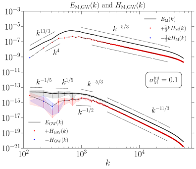
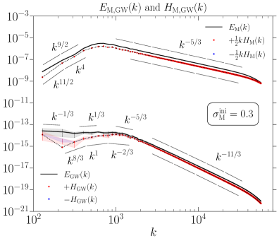
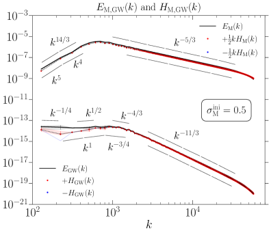
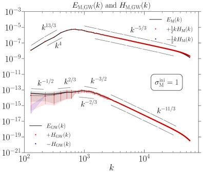
Figure 1: Magnetic and GW energy (solid lines) and helicity (dashed lines) spectra for the runs with a magnetic field given at the initial time of the simulations, normalized to $t_{*}=1$, for different values of the parameter $\sigma_{\rm M}$, which is related to the fractional magnetic helicity as ${\cal P}_{\rm M}=2\sigma_{\rm M}/(1+\sigma_{\rm M}^{2})$. The magnetic spectra are shown at the initial time of the simulation and the GW spectra are the saturated ones (averaged over times $t>1.01$), while the shaded region shows the variation over time between the maxima and minima. Positive values of the helicity spectra (magnetic and GW) are shown in red, while negative values in blue. The discretized intervals show the tangent power laws fitting the spectra used to compute their local slopes, shown as a fraction of integers, with a tolerance of $0.1$. The values of the wave numbers and spectra are comoving and normalized by the Hubble rate and the radiation energy density at the initial time, respectively.

In figure 1, we compare the spectra of the magnetic field and the resulting GWs, both the symmetric, $E_{\rm M}(k)$ and $E_{\rm GW}(k)$, and the antisymmetric spectra, $H_{\rm M}(k)$ and $H_{\rm GW}(k)$, for different values of $\sigma_{\rm M}$ at the initial time of the simulation. Since the GW spectra fluctuate around an approximately statistically steady spectrum, we show the saturated values of the spectra at each mode computed by averaging them over times larger than $t=t_{*}+1/k_{0}=1.01$, and the shaded region corresponds to the maxima and minima of the oscillations at every wave number. The magnetic spectra are shown at the initial time of the simulation, when the magnetic energy density has its maximum ${\cal E}_{\rm M}^{\rm max}$, and it decays for later times.

The magnetic helicity spectrum shows the same power law scalings as the spectrum of the magnetic energy density in the inertial range, which correspond to $k^{-5/3}$ Kolmogorov-type spectra. Thus, this corresponds to HT turbulence; see section 3.4. In the subinertial range, we observe that, as we decrease the fractional helicity, the helical spectrum becomes slightly steeper than the $k^{4}$ Batchelor spectrum observed in the magnetic energy density, being both spectra identical in the fully helical case, as expected. Note that the magnetic helicity spectra are multiplied by $k/2$ to take into account the realizability condition; see equation (2.13).

On small length scales or, equivalently, large wave numbers (above the spectral peak $k_{*}$), we observe that both the GW energy density and helicity spectra, $E_{\rm GW}(k)$ and $H_{\rm GW}(k)$, follow $k^{-11/3}$ scalings, which correspond to the Kolmogorov-type magnetic spectra, in agreement with ref. [82]. On larger scales, we observe an approximately flat spectrum for the GW energy, as shown from numerical simulations in ref. [82]. This is a consequence of the $k^{4}$ Batchelor spectrum for a Gaussian magnetic (hence, divergenceless) field, which yields a $k^{2}$ (i.e., white noise) spectrum of the magnetic stress [82, 96]. The small deviations from an exact flat spectrum, which increase towards negative slopes as we decrease the value of the fractional helicity, could be due to the small number of points in wave number space when we reach the largest scales of the simulation, as well as to the oscillations over time. It is also for large scales (small wave numbers) that we observe a decay of the GW helical spectrum $H_{\rm GW}(k)$ with respect to the flat spectrum observed for $E_{\rm GW}(k)$. As we decrease the fractional helicity of the magnetic field, we observe this decay to be at approximately twice the smallest wave number of the magnetic field (expected from the source of the GWs that is given through convolution). This could be due to the steeper slope of the helical magnetic spectrum at low wave numbers, impacting the helical spectrum of GWs. Hence, we can expect the helicity spectrum of GWs to decay with respect to the flat spectrum in the subinertial range, and omit the smallest wave number of the simulation $k_{0}$, since the correct computation of this mode would require the computation of the magnetic field at $k_{0}/2$. We defer further discussion of the GW polarization ${\cal P}_{\rm GW}(k)=H_{\rm GW}(k)/E_{\rm GW}(k)$ to sections 3.3 and 3.4.

3.2 Runs with forced magnetic field at the initial time

In figures 2 and 3, we compare the spectra of the magnetic field and the resulting GWs for the runs in which we drive the magnetic field for a short duration $\delta t=t_{\rm max}-1=0.1$ (i.e., 10% of the Hubble time). In figure 2, we show runs that are almost non-helical ($\sigma_{\rm M}=\pm 0.01$), and in figure 3, we show runs with larger fractional helicity of the forcing term, up to the fully helical case (which is negative in this case). We show that magnetic fields with negative helicity drive GW with the same GW energy density than those produced by magnetic fields with positive helicity, but the resulting helicity of the GW spectrum is negative. The time evolution of the fractional magnetic helicity ${\cal P}_{\rm M}(t)$ is shown in figure 4. We observe that at very early times (up to $\delta t\approx 2\times 10^{-2}$ for the runs with $\sigma_{\rm M}=0.3$ and $0.5$, and up to $\delta t\approx 10^{-1}$ for the other runs), the value of $\sigma_{\rm M}$ corresponds to the parameter $\sigma$ of the forcing term.

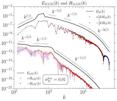
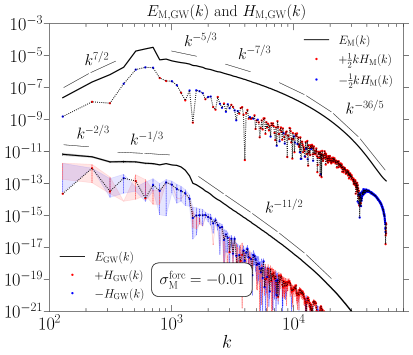
Figure 2: Magnetic and GW energy (solid lines) and helicity (dashed lines) spectra, similar to figure 1, for runs with an almost non-helical forcing ($\sigma_{\rm M}=\pm 0.01$) for short times ($1\leq t\leq 1.1$).

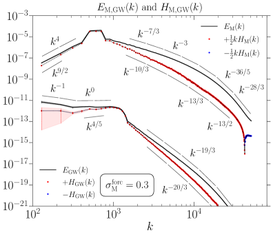
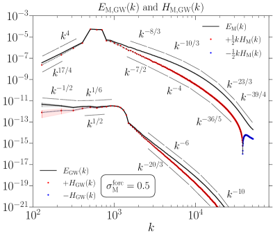
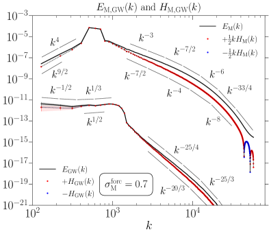
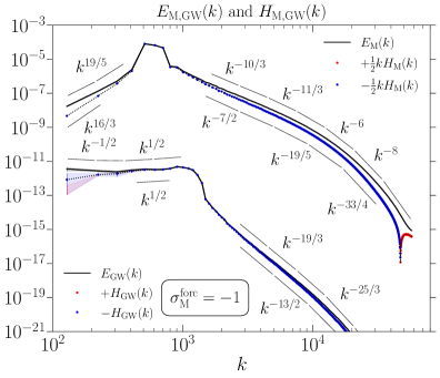
Figure 3: Magnetic and GW energy (solid lines) and helicity (dashed lines) spectra, similar to figure 1, for runs with forcing for short times ($1\leq t\leq 1.1$), for different values of $\sigma_{\rm M}$.

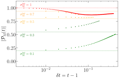
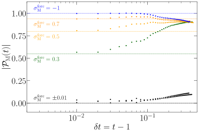
Figure 4: Time evolution of the fractional helicity of the magnetic field, for the different values of $\sigma_{\rm M}$, for (a) the runs with an initial given magnetic field, and (b) those with a forced magnetic field.

The magnetic spectra are shown at the time $t_{\rm max}$, when the magnetic energy density reaches its maximum value ${\cal E}_{\rm M}^{\rm max}$, and when we switch off the forcing term. Note that at $t_{\rm max}=1.1$; see figure 4, the value of the fractional magnetic helicity is dynamically evolving in time, and is already different than its initial value. At earlier times, the magnetic spectrum shows a spike around the forcing wave number $k_{*}$, which is distributed at later times to a turbulent spectrum due to the MHD dynamical evolution of the magnetic field. We see that in all cases, the causal $E_{\rm M}(k)\propto k^{4}$ magnetic spectrum is established. The spectra are averaged over times $t\geq 1.1$, which is just after the maximum magnetic energy has been reached and the GW energy begins to fluctuate around an approximately statistically steady state. For $k>k_{*}$, the slope of the magnetic energy spectrum is steeper than a $k^{-5/3}$ Kolmogorov-type spectrum. This is because of the finite time driving during the rather short time interval, $1\leq t\leq 1.1$. The consequences of the finite forcing time are the appearance of a smoothed spike around $k_{*}$ which has not completely disappeared, and the steeper slopes, especially in the inertial range. This effect seems to be enhanced with helicity. An exponential drop in the magnetic spectra is observed at the largest wave numbers due to viscosity and magnetic diffusivity. We can estimate the viscous cutoff wave number $k_{\nu}$ from the energy dissipation rate $\epsilon\sim\nu\langle\omega^{2}\rangle$, where $\mathchoice{\mbox{\boldmath$\displaystyle\omega$}}{\mbox{\boldmath$\textstyle\omega$}}{\mbox{\boldmath$\scriptstyle\omega$}}{\mbox{\boldmath$\scriptscriptstyle\omega$}}{}=\mathchoice{\mbox{\boldmath$\displaystyle\nabla$}}{\mbox{\boldmath$\textstyle\nabla$}}{\mbox{\boldmath$\scriptstyle\nabla$}}{\mbox{\boldmath$\scriptscriptstyle\nabla$}}{}\times\mathchoice{\mbox{\boldmath$\displaystyle u$}}{\mbox{\boldmath$\textstyle u$}}{\mbox{\boldmath$\scriptstyle u$}}{\mbox{\boldmath$\scriptscriptstyle u$}}{}$ is the fluid vorticity, as $k_{\nu}\sim(\epsilon/\nu^{3})^{1/4}$ (see table 1). Note that for the runs with a given initial magnetic field, the diffusive scale is around the Nyquist wave number so the inertial range is observed down to the smallest scales of the simulation. If the driving was continued over a long time interval (long enough for the magnetic field to be processed, i.e., $t_{\rm max}\sim 1$) we would recover the Kolmogorov spectrum [65]. The magnetic helicity spectrum around the peak $k_{*}$ is nearly saturated for all values of $|\sigma_{\rm M}|$ considered from 0.3 to 1. For $\sigma_{\rm M}=\pm 0.01$, there is a clear separation between $E_{\rm M}(k)$ and $kH_{\rm M}(k)/2$ and the sign of the magnetic helicity tends to fluctuate noticeably, especially at high wave numbers. We also see a systematic sign flip at higher $k$ both in $H_{\rm M}(k)$ and $H_{\rm GW}(k)$, which also occurs for the cases with $|\sigma_{\rm M}|\geq 0.3$. Such sign flips are typical of decaying helical turbulence and are a consequence of the fact that the fractional magnetic helicity is there already extremely small. The helicity spectrum $kH_{\rm M}(k)$ is steeper than the magnetic spectrum $E_{\rm M}(k)$, while in the runs with an initial magnetic field, both spectra follow the same power laws in the inertial range. This is observed for all values of $\sigma_{\rm M}$. However, for the fully helical case, the difference in slope is smaller, and it becomes larger for smaller fractional helicity.

We again observe an approximately flat GW spectrum in the subinertial range, which presents negative slopes that become steeper for smaller values of $|\sigma_{\rm M}|$. For values of $|\sigma_{\rm M}|\geq 0.3$, the spectrum becomes completely flat near the spectral peak, and then presents an abrupt drop below the peak, as shown in ref. [82], which is due to the finite duration of the forcing, and related to the spike that appears in the magnetic spectra. The inertial range of the GW spectra also present steeper slopes than the $k^{-11/3}$ obtained for the Kolmogorov scaling in the case of initially given magnetic fields. We observe the slopes $-5.5$, $-6.33$, $-6$, $-6.25$, and $-6.33$ below the spectral peak for $\sigma_{\rm M}=\pm 0.01$, $0.3$, $0.5$, $0.7$, and $-1$, respectively. The helical GW spectrum is slightly shallower on small scales, and becomes fully helical around the spectral peak. Similar to the magnetic field, the helical GW spectrum decays faster than the GW energy density in the subinertial range after a characteristic wave number that increases with the fractional magnetic helicity. We observe that this decay starts at larger wave numbers for the GW spectra than for the magnetic spectra.

3.3 Degree of circular polarization

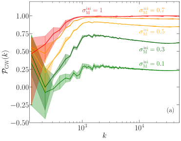
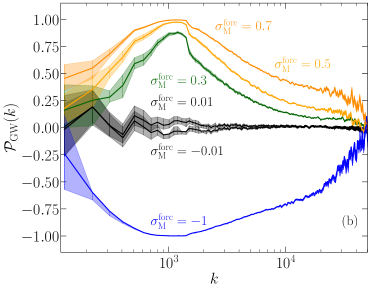
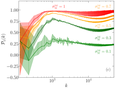
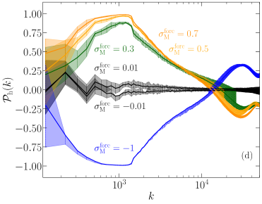
Figure 5: GW degree of circular polarization, ${\cal P}_{h}(k)$ and ${\cal P}_{\rm GW}(k)$, for the different values of $\sigma_{\rm M}$, for the types of simulations: runs with a given initial field; see panels (a) and (c), and runs with a forced magnetic field for a short duration, i.e., for times $1\leq t\leq 1.1$; see panels (b) and (d). The solid line represents the saturated value of the polarization (i.e., averaged over times in the oscillatory regime), and the shaded regions are the maximum and minimum values of the polarization over oscillations.

In figure 5, we plot the GW degree of circular polarization, ${\cal P}_{h}(k)$ and ${\cal P}_{\rm GW}(k)$, for the two types of simulations. We see that ${\cal P}_{\rm GW}(k)$ reaches $\pm 1$ at the GW spectral peak $k_{\rm GW}\approx 2k_{*}\approx 1200$ when $\sigma_{\rm M}=\pm 1$. This polarization is larger than what was found in previous analytic predictions; see ref. [63], and recently used in ref. [64] in relation to detectability with LISA. This discrepancy can probably be explained by the use of the simplified approximations made in the analytic calculations. Toward smaller wave numbers, there are systematic fluctuations around ${\cal P}_{\rm GW}(k)=0$, especially in the case of an initial given magnetic field, due to the oscillations of the helical GW spectrum at low wave numbers.

The GW polarization integrated over all wave numbers ${\cal P}_{\rm GW}$, as a function of the magnetic fractional helicity ${\cal P}_{\rm M}=2\sigma_{\rm M}/(1+\sigma_{\rm M}^{2})$, is shown in figure 6. The value of the integrated magnetic fractional helicity ${\cal P}_{\rm M}$, as a function of time is shown in figure 4. In the runs with an initial given magnetic field, ${\cal P}_{\rm M}$ stays constant for a short time interval $\delta t=t-1\sim 10^{-2}$, which is similar to the time that the GW spectrum takes to enter the stationary regime. Hence, the value of ${\cal P}_{\rm M}$ does not change while the GW spectrum is established. However, for the case in which the magnetic field is driven for a duration $\delta t_{\rm max}=t_{\rm max}-1=10^{-1}$, the fractional helicity ${\cal P}_{\rm M}$ has changed more significantly when the GW spectrum is established, such that the variation of helicity affects the GW polarization; see figures 2 and 3. At earlier times, as mentioned in section 3.2, the values of $\sigma_{\rm M}$ are the same as the values of the parameter $\sigma$ of the forcing term. We observe a dependence ${\cal P}_{\rm GW}\sim{\cal P}_{\rm M}$, inferred from the numerical results; see figure 6. This result differs from the analytical model considered in Appendix A, which corresponds to a magnetic field that depends only on one spatial coordinate with fractional helicity ${\cal P}_{\rm M}=2\sigma_{\rm M}/(1+\sigma_{\rm M}^{2})$. The predicted dependence of the degree of circular polarization is ${\cal P}_{\rm GW}=2{\cal P}_{\rm M}/(1+{\cal P}_{\rm M}^{2})$, given in equation (A.21), and shown in figure 14.

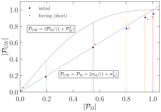
Figure 6: GW polarization ${\cal P}_{\rm GW}$ versus magnetic polarization ${\cal P}_{\rm M}$; see table 1. We obtain a numerical fit ${\cal P}_{\rm GW}\approx{\cal P}_{\rm M}=2\sigma_{\rm M}/(1+\sigma_{\rm M}^{2})$, both for the runs with an initial given magnetic field (‘initial’), and with an initially driven field (‘forcing (short)’). We compare with the relation obtained for the analytical model of Appendix A, ${\cal P}_{\rm GW}=2{\cal P}_{\rm M}/(1+{\cal P}_{\rm M}^{2})$; see equation (A.21). The vertical lines correspond to $|\sigma_{\rm M}|=0.1$ (green), $0.3$ (dark green), $0.5$ (orange), $0.7$ (dark orange), and $1$ (red).

3.4 Comparison to the analytical prediction of the spectrum of polarization

The GW degree of circular polarization of signals produced by primordial MHD turbulence has been estimated in refs. [62, 63]. In this section, we use their model to predict the spectrum of GW polarization ${\cal P}_{h}$ and compare it to the numerical results, to explore the validity of their model and the impact of the assumptions made. In the first place, we define the unequal time correlation (UTC) function of the magnetic field as

$$\langle\tilde{B}_{i}(\mathchoice{\mbox{\boldmath$\displaystyle k$}}{\mbox{\boldmath$\textstyle k$}}{\mbox{\boldmath$\scriptstyle k$}}{\mbox{\boldmath$\scriptscriptstyle k$}}{},t_{1})\tilde{B}^{*}_{j}(\mathchoice{\mbox{\boldmath$\displaystyle k$}}{\mbox{\boldmath$\textstyle k$}}{\mbox{\boldmath$\scriptstyle k$}}{\mbox{\boldmath$\scriptscriptstyle k$}}{}^{\prime},t_{2})\rangle=(2\pi)^{6}\delta^{3}(\mathchoice{\mbox{\boldmath$\displaystyle k$}}{\mbox{\boldmath$\textstyle k$}}{\mbox{\boldmath$\scriptstyle k$}}{\mbox{\boldmath$\scriptscriptstyle k$}}{}-\mathchoice{\mbox{\boldmath$\displaystyle k$}}{\mbox{\boldmath$\textstyle k$}}{\mbox{\boldmath$\scriptstyle k$}}{\mbox{\boldmath$\scriptscriptstyle k$}}{}^{\prime})\left(P_{ij}(\hat{\mathchoice{\mbox{\boldmath$\displaystyle k$}}{\mbox{\boldmath$\textstyle k$}}{\mbox{\boldmath$\scriptstyle k$}}{\mbox{\boldmath$\scriptscriptstyle k$}}}{})\frac{F_{\rm M}(k,t_{1},t_{2})}{4\pi k^{2}}+i\varepsilon_{ijl}\hat{k}_{l}\frac{G_{\rm M}(k,t_{1},t_{2})}{8\pi k}\right),$$ (3.1)

where we recover the equal time correlation of the magnetic energy density and helicity, defined in equation (2.11), when $t_{1}=t_{2}=t$, $F_{\rm M}(k,t,t)=E_{\rm M}(k,t)$, and $G_{\rm M}(k,t,t)=H_{\rm M}(k,t)$. Following ref. [62], which assumes stationary turbulence, we express the spectral functions of the UTC of the freely decaying turbulent source as a function of only the time difference, modelled as $F_{\rm M}(k,t_{1},t_{2})=F_{\rm M}(k,t_{1},t_{1}+\delta t)\approx E_{\rm M}(k,t_{1})D_{1}(\delta t)$. Similarly, the helical contribution to the UTC spectrum is $G_{\rm M}(k,t_{1},t_{2})=G_{\rm M}(k,t_{1},t_{1}+\delta t)\approx H_{\rm M}(k,t_{1})D_{2}(\delta t).$ The functions $D_{1}(\delta t)$ and $D_{2}(\delta t)$ are monotonically decreasing functions, with $D_{1}(0)=D_{2}(0)=1$. To characterize the two types of turbulence considered in the present work, $t_{1}$ is considered to be the time when the turbulence starts freely decaying. This corresponds to the initial time ($t_{1}=1$) for the cases with a given magnetic field, and to the time at which the forcing term is switched off ($t_{1}=t_{\rm max}$) otherwise.

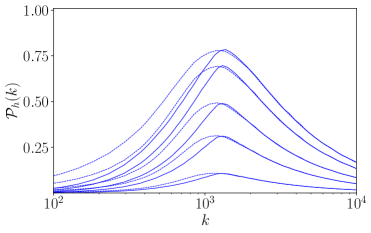
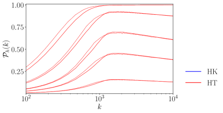
Figure 7: Polarization spectra ${\cal P}_{h}(k)$ for HK turbulence with $n_{\rm S}=-5/3$ and $n_{\rm A}=-8/3$ in the subinertial range (blue), and for HT turbulence with $n_{\rm S}=n_{\rm A}=-5/3$ (red), using a single power law in the inertial range (solid lines) [62, 63, 64], and using a broken power law with a Batchelor spectrum in the subinertial range (dotted lines), for fractional helicities $h=0.1$, $0.3$, $0.5$, $0.8$, and $1$. We use $k_{*}=600$ for comparison with the numerical simulations.

Assuming that the duration of the turbulence sourcing is short, i.e., $\tau=t_{\rm fin}-1\ll 1$, where $t_{\rm fin}$ corresponds to the final time of the turbulence, such that the expansion of the universe can be neglected, and after averaging over the time oscillations of the source, the functions $S_{h}(k)$ and $A_{h}(k)$ can be obtained as [62, 11]

$$S_{h}(k)=A\frac{\tau}{k^{2}}\int{\rm d}{}\ln p_{1}\int{\rm d}{}\ln p_{2}\bar{\Theta}\Big{[} (1+\gamma^{2})(1+\beta^{2})E_{\rm M}(p_{1})E_{\rm M}(p_{2})$$

$$+4\gamma\beta H_{\rm M}(p_{1})H_{\rm M}(p_{2})\Big{]},$$ (3.2)

$$A_{h}(k)=2A\frac{\tau}{k^{2}}\int{\rm d}{}\ln p_{1}\int{\rm d}{}\ln p_{2}\bar{\Theta}\Big{[} (1+\gamma^{2})\beta E_{\rm M}(p_{1})H_{\rm M}(p_{2})$$

$$+(1+\beta^{2})\gamma H_{\rm M}(p_{1})E_{\rm M}(p_{2})\Big{]},$$ (3.3)

where $\bar{\Theta}=\Theta(p_{1}+p_{2}-k)\Theta(p_{1}+k-p_{2})\Theta(p_{2}+k-p_{1})$, $\gamma=(k^{2}+p_{1}^{2}-p_{2}^{2})/(2kp_{1})$, $\beta=(k^{2}+p_{2}^{2}-p_{1}^{2})/(2kp_{2})$, and $A$ is a constant that we omit, since we are interested in the spectral shapes, and we will use equations (3.2) and (3.3) to compute the polarization, which does not depend on $A$. Previous analytical assumptions [62, 63, 64] consider two types of turbulence:

• Helical Kolmogorov (HK) turbulence driven by magnetic energy dissipation at small scales, resulting in spectral powers $n_{\rm S}=-5/3$ and $n_{\rm A}=-8/3$.

• Turbulence determined by helical transfer (HT) and helicity dissipation at small scales, which results in $n_{\rm S}=n_{\rm A}=-7/3$, based in ref. [78].

They use power law spectra $E_{\rm M}(k)\propto k^{n_{\rm S}}$ and $kH_{\rm M}(k)\propto hk^{n_{\rm A}}$ in the range $k_{*}<k<k_{\nu}$, with $h$ being the fraction of helicity dissipation. We extend their analytic approach to consider a broken power law with a subinertial $k^{4}$ Batchelor spectrum below $k_{*}$, and modify the HT spectrum to $n_{\rm S}=n_{\rm A}=-5/3$, corresponding to the spectral slopes of the stochastic magnetic fields that we use in our numerical simulations (see figure 1) and that is based in previous MHD simulations applied to cosmological phase transitions [39]. Figure 7 shows the resulting polarization degree ${\cal P}_{h}(k)$ for the HT and HK types of turbulence. The inclusion of the subinertial range leads to an increase on polarization at wave numbers right below the peak, which is a more realistic scenario when compared to the numerical results, especially for the case of HK turbulence. The model described above assumes that the partial helicity at $k_{*}$ is ${\cal P}_{\rm M}(k_{*})=h$, and describes the magnetic energy and helicity spectra using power laws. The assumption that the slopes are the same along the inertial range is accurate in the case with an initial magnetic field; see figures 1 and 8.

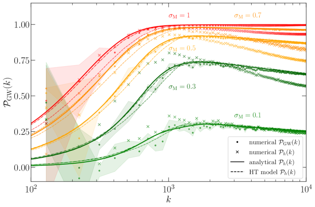
Figure 8: Polarization spectra ${\cal P}_{\rm GW}(k)$ (dots) and ${\cal P}_{h}(k)$ (crosses) obtained from the numerical simulations for different $\sigma_{\rm M}$, compared to ${\cal P}_{h}(k)$ computed from the analytical model (single power law and extended to a broken power law; see figure 7) using HT type of turbulence (dashed lines), and from the analytical integrals; see equations (3.2) and (3.3), using the numerical spectra of the turbulence (solid lines). Similar to figure 6, the shaded regions denote the maximum and minimum polarizations ${\cal P}_{\rm GW}(k)$ of the fluctuations.

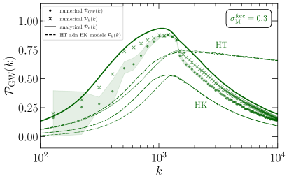
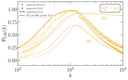
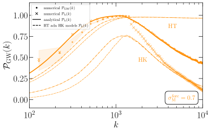
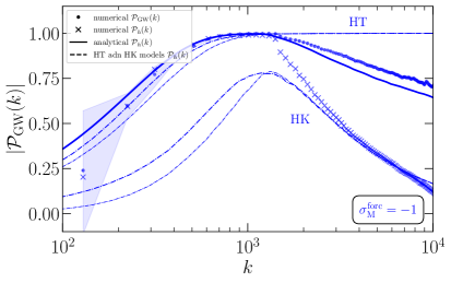
Figure 9: Similar to figure 8, polarization spectra ${\cal P}_{\rm GW}(k)$ and ${\cal P}_{h}(k)$ obtained from the numerical simulations for different $\sigma_{\rm M}$, compared to ${\cal P}_{h}(k)$ obtained from the analytical model using both HK and HT types of turbulence (dashed lines; see figure 7), and obtained from the analytical integral, using the numerical spectrum of the turbulence (solid lines).

In figure 8, we compare the analytical results obtained from HT turbulence (with modified slopes and extended to broken power laws; see figure 7) with our numerical simulations that consider an initial given magnetic field. Note that the extension of the turbulent spectra to $k<k_{*}$ allows one to get a more accurate position of the polarization spectral peak. In general, we observe good agreement of the analytical results with the polarization ${\cal P}_{\rm GW}(k)$ computed from the simulations, while the spectrum ${\cal P}_{h}(k)$ agrees well at low and intermediate $k$, but decays with respect to the analytical models for large $k$. However, in the case in which the magnetic field is forced for a short duration of time, we observe in figure 3 that the energy and helicity spectra are similar around the spectral peak (where the magnetic field is maximally helical), while the helical spectrum starts decaying with a steeper slope than the magnetic spectrum at a specific wave number, which increases with the helicity of the forcing. This behavior is not captured by previous analytical models. In figure 9, we compare the results of the polarization spectra ${\cal P}_{h}(k)$ and ${\cal P}_{\rm GW}(k)$, obtained from the numerical simulations, with those obtained from HK and HT types of turbulence. In addition, to take into account the deviations from the assumption of constant slopes of the magnetic spectra, we compute the polarization using equations (3.2) and (3.3) by integrating over the numerically computed spectra $E_{\rm M}(k)$ and $H_{\rm M}(k)$. We observe in figures 8 and 9 that the latter gives an accurate approximation of ${\cal P}_{\rm GW}(k)$ to the numerical results, while ${\cal P}_{h}(k)$ shows a bigger decay at large $k$. In general, the polarization spectrum shows features of both HK and HT types of turbulence. As we have mentioned, around the spectral peak, the numerical simulations show that the magnetic field is maximally helical in all the considered runs with $|\sigma_{\rm M}|\geq 0.3$ or $|{\cal P}_{\rm M}|\geq 0.55$, which is better represented by the HT spectrum (with $h=1$) in the subinertial range, while in the inertial range the different slopes lead to a decrease of the polarization with a scaling similar to that of the HK spectrum, especially as we decrease the fractional helicity, although the polarization computed numerically is still larger than that obtained by the HK model in all cases.

We have confirmed using numerical simulations that in the case of an initial magnetic field with a Kolmogorov spectrum for both the magnetic energy density and helicity, the analytical model previously considered in refs. [62, 63, 64] using HK turbulence gives an accurate prediction of the degree of circular polarization, which gets better when we consider a broken power law. However, when we consider the scenario in which the magnetic field is generated via MHD forcing for a short amount of time, and non-linear interactions appear, allowing to have different spectral slopes at different scales, previous analytical estimates underpredict considerably the polarization degree peak and fail to predict the appropriate shape, which is not given by either the HK or the HT models, but presents non-linearly combined features of both. In addition, we observe a helical inverse cascade that produces larger degree of circular polarization at large scales.

4 Prospects of detecting signals from the electroweak phase transition

4.1 Observable GW energy density spectra

The GW energy density at the present time is obtained from the comoving ${\Omega}_{\rm GW}(k)$, defined in equation (2.19), and expressed as a function of the frequency. For a signal that has been produced at the EWPT, the resulting GW spectrum is

$${\Omega}_{\rm GW}(k)= \,\left(\frac{a_{0}}{a_{*}}\right)^{-4}\left(\frac{H_{*}}{H_{0}}\right)^{2}kE_{\rm GW}(k),$$

$$h_{0}^{2}\,{\Omega}_{\rm GW}(f)= \,1.652\times 10^{-5}\left(g_{*}/100\right)^{-1/3}\left(2\pi f/f_{\rm H}\right)E_{\rm GW}(f),$$ (4.1)

where we have used the present time values $T_{0}=2.73\,{\rm K}$, $g_{0}=3.91$, and $H_{0}$, expressed by the Hubble parameter today $h_{0}$ in units of $100\,{\rm km}\,{\rm s}^{-1}\,{\rm Mpc}^{-1}$ [94], and $g_{*}$ and $f_{\rm H}=H_{*}a_{*}/a_{0}$ are the number of degrees of freedom and the Hubble frequency, respectively, at the electroweak scale. The ratio of the scale factors is obtained assuming adiabatic expansion, i.e., with constant $g\,T^{3}a^{3}$ [97],

$$\frac{a_{0}}{a_{*}}=1.254\times 10^{15}\left(\frac{k_{\rm B}T_{*}}{100\,{\rm GeV}}\right)\left(\frac{g_{*}(T_{*})}{100}\right)^{1/3},$$ (4.2)

with $T_{*}$ being the electroweak temperature. The Hubble rate at the electroweak scale is [97]

$$H_{*}=2.066\times 10^{10}\,{\rm s}^{-1}\left(\frac{k_{\rm B}T_{*}}{100\,{\rm GeV}}\right)^{2}\left(\frac{g_{*}(T_{*})}{100}\right)^{1/2}.$$ (4.3)

The resulting spectrum is expressed in terms of the frequency, which corresponds to the physical comoving wave number (from the GW dispersion relation $2\pi f=k$) shifted to the present time; see ref. [97],

$$f=\frac{H_{*}}{2\pi}\left(\frac{a_{*}}{a_{0}}\right)k=\frac{f_{\rm H}}{2\pi}k,\quad\text{with }f_{\rm H}=1.646\times 10^{-5}\,{\rm Hz}\left(\frac{k_{\rm B}T_{*}}{100\,{\rm GeV}}\right)\left(\frac{g_{*}(T_{*})}{100}\right)^{1/6},$$ (4.4)

being the Hubble frequency at the electroweak scale, which corresponds to $k_{\rm H}=2\pi$ according to our normalization. The helical spectrum of GWs $h_{0}^{2}\,{\Xi}_{\rm GW}(f)$, defined in equation (2.20), is computed in the same way as $h_{0}^{2}{\Omega}_{\rm GW}(f)$ in equation (4.1), substituting $E_{\rm GW}(k)$ by $H_{\rm GW}(k)$.

Recent numerical simulations of GWs produced by MHD turbulence have found a dependence of the GW energy density ${\Omega}_{\rm GW}$ on the square of the magnetic energy density ${\cal E}_{\rm M}^{2}$ and the inverse of the square of the magnetic spectral peak $k_{*}^{-2}$ [82, 65, 98, 99]; see equation (2.15). In the present work, our numerical simulations follow this scaling, and we define the GW efficiency $q^{2}(t)=k_{*}^{2}{\Omega}_{\rm GW}(t)/({\cal E}_{\rm M}^{\rm max})^{2}$, shown in figure 10. Such scaling was obtained in early analyses of MHD turbulent production of GWs; see, e.g., refs. [10, 11, 12, 13], which assumed stationary turbulence, and reported in ref. [100] in the case when the decay of the magnetic field does not impact the evolution of GWs. We compute this scaling in the analytical model presented in Appendix A; see also the Beltrami field studied in ref. [83]. However, ref. [100] proposes a general ${\cal E}_{\rm M}^{3/2}$ scaling for MHD turbulence; see their equation (82), which was previously obtained in refs. [101, 102], and assumes that the magnetic field decay impacts the GW dynamics. This is often used when considering GW signals from MHD turbulence in the LISA band [18]. In general, the exact scaling depends on the dynamical evolution of the magnetic field and, in particular, on the UTC of the stress, which is modelled in previous estimates (see reviews [103, 25]), while the direct numerical simulations of MHD turbulence allow to obtain the final GW spectrum with no assumptions on the magnetic stress UTC.

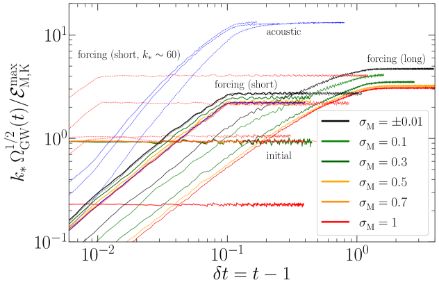
Figure 10: Efficiency of GW energy density $q(t)=k_{*}{\Omega}_{\rm GW}^{1/2}(t)/{\cal E}_{i}^{\rm max}$ for $i=$ M (magnetic) and K (kinetic) in units of $a^{-4}(H_{*}/H_{0})^{2}=1.644\times 10^{-5}\,(g_{*}/100)^{-1/3}$; see equations (2.15) and (4.1), for the runs with an initial given magnetic field (‘initial’), and for the runs with a forced magnetic field (‘forcing (short)’), with $t_{\rm max}=1.1$. Added for comparison are the runs in ref. [65] (‘forcing (long)’), in which the magnetic field is forced for longer times ($t_{\rm max}=3$), and the runs of ref. [82], which contain cases with initial given magnetic field, with forced magnetic field at $k_{*}=60$, $600$, and $6000$, and runs of acoustic turbulence (‘acoustic’).

We observe that the GW production is similar for all values of $\sigma_{\rm M}$ if the magnetic field is present at the initial time of generation with a GW efficiency of $q=0.95$. For the case in which the magnetic field is forced at initial times, we observe an enhancement of the GW production by a factor of $\sim 5$, and larger GW energy densities for smaller helicities. The dependency of the GW production on the helicity is consistent with that for the runs of ref. [65], in which the forcing term is present for longer times, and the GW production is larger. In the case of acoustic turbulence (e.g., sound waves), the GW production is larger by a factor of $\sim 200$, as reported in ref. [82]. The GW production obtained in the numerical simulations is smaller than the estimated amplitudes computed in previous analytical estimates [104, 64]. This is probably due to simplifying assumptions made. We defer the study of the scaling of the GW amplitudes with the characteristic scale and the amplitude of the turbulence sourcing to future work.

4.2 Interferometry of GW detectors LISA and Taiji

The GW signals produced at the EWPT are expected to be detectable with future planned space-based GW detectors, e.g., LISA [7], Taiji [9], TianQin [8], DECIGO [19], and BBO [21]. We revisit the interferometry of this type of detectors in Appendix B, and apply the analysis to LISA and Taiji to consider the potential detectability of the circular polarization of GW signals produced by primordial magnetic fields. In general, it is necessary that the GW background presents anisotropies to measure its circular polarization [66, 67]. Hence, a priori, parity-violating effects cannot be detected if the system of GW detectors is coplanar, which is the case for space-based GW detectors, and the GW background is isotropic [105]. However, different approaches have recently been proposed to detect the circular polarization of a statistically isotropic GW background [79, 80, 81]. On the one hand, a statistically isotropic GW background, such as that expected from cosmological sources, can present anisotropies that have been kinematically induced due to the proper motion of the solar system, and the induced anisotropies allow one to detect the circular polarization of the background [66, 67]. On the other hand, the combination of a network of GW detectors breaks the coplanarity of the detectors allowing one to detect circular polarization. This has been considered in the case of ground-based GW detectors; see, e.g., refs. [106, 105, 107, 108, 79], and for the LISA–Taiji network [80, 81].

The total and the polarization signal-to-noise ratios (SNR) of a stochastic GW background with energy density ${\Omega}_{\rm GW}(f)$ and helical spectra ${\Xi}_{\rm GW}(f)$, for a duration $T$ of the observations, are

$${\rm SNR}= \,2\sqrt{T}\left[\int_{0}^{\infty}{\rm d}{}f\left(\frac{{\Omega}_{\rm GW}(f)}{\Omega_{\rm s}(f)}\right)^{2}\right]^{1/2},$$ (4.5)

$${\rm SNR}_{\rm pol}^{\rm dip}= \,2\sqrt{T}\left[\int_{0}^{\infty}{\rm d}{}f\left(\frac{{\Xi}_{\rm GW}(f)-{\textstyle{1\over 4}}{\rm d}{}{\Xi}_{\rm GW}(f)/{\rm d}{}\ln f}{\Xi_{\rm s}^{\rm dip}(f)}\right)^{2}\right]^{1/2},$$ (4.6)

$$\ {\rm SNR}_{\rm pol}^{\text{comb}}= \,2\sqrt{T}\left[\int_{0}^{\infty}{\rm d}{}f\left(\frac{{\Xi}_{\rm GW}(f)}{\Xi_{\rm s}^{\rm comb}(f)}\right)^{2}\right]^{1/2},$$ (4.7)

where the GW sensitivity $\Omega_{\rm s}(f)$ in equation (4.5) refers to LISA, $\Omega_{\rm s}^{A}(f)$, Taiji, $\Omega_{\rm s}^{C}(f)$, or the combined LISA–Taiji network, $\Omega_{\rm s}^{\rm comb}(f)$; see equations (B.28) and (B.37). The polarization ${\rm SNR}_{\rm pol}$ given in equation (4.6) is obtained by using the anisotropies induced by the polarization of the GW background, due to our proper motion, yielding a dipolar response in the LISA $A$ and $E$ channels or the Taiji $C$ and $D$ channels, with the sensitivity $\Xi_{\rm s}^{\rm dip}(f)=\Xi_{\rm s}^{AE}(f)$ or $\Xi_{\rm s}^{CD}(f)$ given in equation (B.29). On the other hand, the polarization ${\rm SNR}_{\rm pol}$ given in equation (4.7) is obtained by cross-correlating the different channels between LISA and Taiji with the sensitivity $\Xi_{s}^{\rm comb}(f)$ given in equation (B.41). Further details on the dipole response function and the LISA–Taiji cross-correlations are given in Appendices B.3 and B.4, respectively, and the GW sensitivity functions are shown in figure 16. Assuming flat GW energy density ${\Omega}_{\rm GW}(f)$ and helicity spectra ${\Xi}_{\rm GW}(f)$ of the background, we get

$$h_{0}^{2}\,{\Omega}_{\rm GW}^{\rm LISA}(f)=h_{0}^{2}\,\Omega_{\rm flat}^{A}= \,1.65\times 10^{-13}\left(\frac{{\rm SNR}}{10}\right)\sqrt{\frac{4\,{\rm yr}}{T}},$$ (4.8)

$$h_{0}^{2}\,{\Omega}_{\rm GW}^{\rm Taiji}(f)=h_{0}^{2}\,\Omega_{\rm flat}^{C}= \,6.81\times 10^{-14}\left(\frac{{\rm SNR}}{10}\right)\sqrt{\frac{4\,{\rm yr}}{T}},$$ (4.9)

$$h_{0}^{2}\,{\Xi}_{\rm GW}^{\rm LISA}(f)=h_{0}^{2}\,\Xi_{\rm flat}^{AE}= \,10^{-10}\left(\frac{{\rm SNR}_{\rm pol}}{10}\right)\sqrt{\frac{4\,{\rm yr}}{T}}\left(\frac{1.23\times 10^{-3}}{v/c}\right),$$ (4.10)

$$h_{0}^{2}\,{\Xi}_{\rm GW}^{\rm Taiji}(f)=h_{0}^{2}\,\Xi_{\rm flat}^{CD}= \,4.16\times 10^{-11}\left(\frac{{\rm SNR}_{\rm pol}}{10}\right)\sqrt{\frac{4\,{\rm yr}}{T}}\left(\frac{1.23\times 10^{-3}}{v/c}\right),$$ (4.11)

where $v$ is the solar system’s proper motion. Using the values of ${\rm SNR}_{\rm pol}=1$, $v/c=10^{-3}$, and $T=3\,{\rm yr}$, we recover the amplitude $h_{0}^{2}\,\Xi_{\rm flat}^{AE}=1.4\times 10^{-11}$, reported in ref. [79]. The exact value of the SNR necessary to claim that the signal is detectable with a large likelihood is not trivial, and requires a detailed analysis that depends on the spectral shape of the GW signal. For a simplified treatment, we follow refs. [110, 109], in which a value of ${\rm SNR}=10$ is proposed. To study the potential detectability of the GW signals produced by primordial turbulence, we compute the power law sensitivities (PLS) [110], assuming a spectral shape defined by a power law of generic slope; see Appendix B. Figure 16 shows the PLS of LISA and Taji, corresponding to the GW energy density, $\Omega_{\rm PLS}^{A}(f)$ and $\Omega_{\rm PLS}^{C}(f)$, and to the helicity, $\Xi_{\rm PLS}^{AE}(f)$ and $\Xi_{\rm PLS}^{CD}(f)$, using the dipole response function, and for the combined LISA–Taiji network, $\Xi_{\rm PLS}^{\rm comb}(f)$. The reconstruction of the signal for more complex spectral shapes is an active topic of research; see, e.g., the review [111] or the work by the LISA cosmology working group [110], and we defer it to future work. In general, the values of the polarized GW signal $h_{0}^{2}\,{\Xi}_{\rm GW}(f)$ that can be detectable by using the dipole response function of a single space-based GW mission, either LISA or Taiji, require very large amplitudes of the magnetic fields generating GWs. Hence, we consider the combination of LISA and Taiji to detect such polarized GW signals, following ref. [81]. Assuming a flat GW polarized spectrum of the background, we get

$$h_{0}^{2}\,{\Xi}_{\rm GW}^{\text{LISA--Taiji}}(f)=h_{0}^{2}\,\Xi_{\rm flat}^{\rm comb}=5.1\times 10^{-13}\left(\frac{{\rm SNR}_{\rm pol}}{10}\right)\sqrt{\frac{4\,{\rm yr}}{T}},$$ (4.12)

which shows an improvement in the potential detectability of the helicity by a factor of $\sim 80$ with respect to the dipole response function of Taiji.

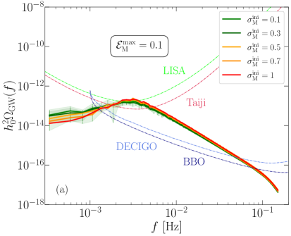
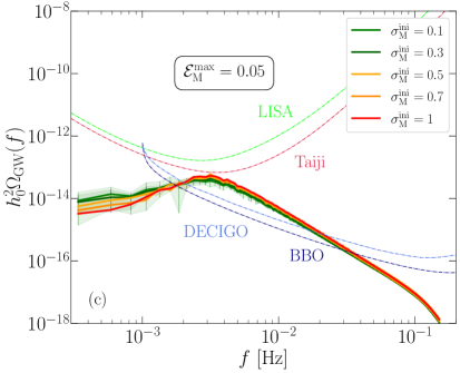
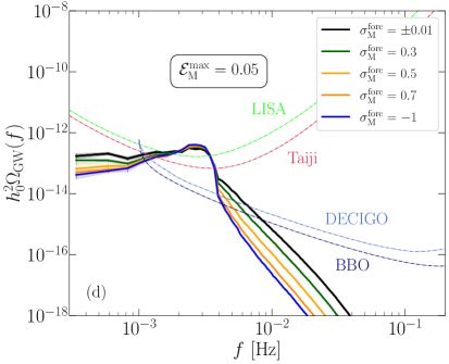
Figure 11: GW spectrum $h_{0}^{2}\,{\Omega}_{\rm GW}(f)$ for signals produced at the EWPT from magnetic fields with ${\cal E}_{\rm M}^{\rm max}=0.1$ for the case with an initial given field (panel a), and the case with a driven field (panel b), and with ${\cal E}_{\rm M}^{\rm max}=0.05$ for both cases (panels c and d). The PLS of the GW detectors assume a SNR of 10 for LISA, Taiji, BBO, and DECIGO, for an observation duration of 4 years; see refs. [110, 113] and figure 16.

4.3 Detectability of GW energy density and polarization

To assess the observational prospects of detecting GWs, we plot in figure 11 the resulting GW signal computed numerically; see section 3, for different values of $\sigma_{\rm M}$, for runs with an initial given magnetic field (left panels) and an initially driven magnetic field (right panels), and compare with the expected PLS of LISA [110], DECIGO, and BBO [113]. We use the results from the numerical simulations; see table 1, shifted to ${\cal E}_{\rm M}^{\rm max}=0.1$ and $0.05$, using the computed ${\cal E}_{\rm M}^{2}$ scaling; see figure 10. The value of $0.1$ has been reported as an upper bound on the combined magnetic, velocity, and GW energy density (as a fraction of the total energy density) from BBN [114, 115]. The spectra are similar, but we now also see that for smaller values of $|\sigma_{\rm M}|$, the jump in ${\Omega}_{\rm GW}(f)$ near the peak is less pronounced, so for larger frequencies, i.e., to the right of the peak, ${\Omega}_{\rm GW}(f)$ increases (decreases) for smaller (larger) values of $|\sigma_{\rm M}|$. For smaller frequencies, we have the aforementioned shallow spectrum ${\Omega}_{\rm GW}(f)\propto f$, which is approximately independent of the value of $\sigma_{\rm M}$. We see that, for an initial magnetic energy density of ${\cal E}_{\rm M}^{\rm max}=0.1$, the GW signal produced is detectable by LISA with a SNR larger than 10 for both types of turbulence. For ${\cal E}_{\rm M}^{\rm max}=0.05$, only the case in which the magnetic field is driven at initial times has a SNR above 10, while the case with an initially given magnetic field has a SNR between 1 and 10.

We show in figure 12 the helicity spectra $|\Xi_{\rm GW}(f)|$ obtained from our numerical simulations together with the PLS obtained using the dipole response function of LISA, and obtained by cross-correlating LISA and Taiji channels. As in figure 11, we shift the numerical GW signal to ${\cal E}_{\rm M}^{\rm max}=0.1$ and $0.05$, according to the scaling ${\Omega}_{\rm GW}(f)\sim{\cal E}_{\rm M}^{2}$. The helical GW spectrum, as the GW energy density, is smaller for the cases in which the magnetic field is given at the initial time than those in which it is initially driven. In this case, since the degree of circular polarization of the GW spectrum is proportional to the magnetic helicity, the fully helical runs result in the largest polarized GW signals. This is clearly seen in the case with initially given magnetic fields. In the driven case, the larger efficiency for smaller fractional magnetic helicity compensates for moderate values of the helicity, and the polarized signal is comparable for all runs with $|\sigma_{\rm M}|\geq 0.3$. Moreover, in the inertial range, since the drop of GW energy is larger for runs with larger helicity, we can observe that the helical GW spectrum becomes smaller for larger values of $|\sigma_{\rm M}|$. We observe that in the limit of a non-helical magnetic field, i.e., $\sigma_{\rm M}=\pm 0.01$, this is no longer the case since the helical spectrum is proportional to the magnetic helicity. In all the cases, we observe that the degree of circular polarization of the GW signals is not large enough to be detectable using the dipolar response function of LISA due to our proper motion.

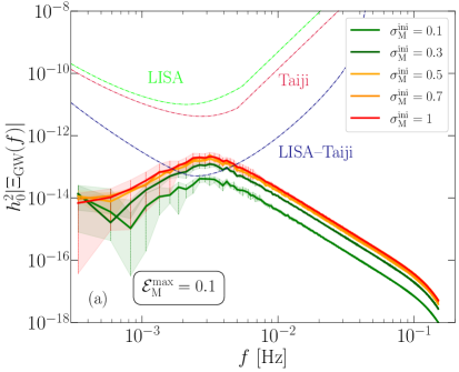
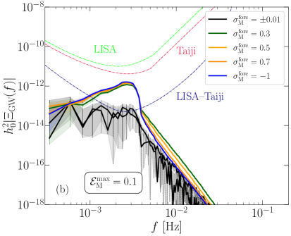
Figure 12: Helical GW spectrum $h_{0}^{2}|{\Xi}_{\rm GW}(f)|$ for signals produced at the EWPT from magnetic fields with ${\cal E}_{\rm M}^{\rm max}=0.1$ for the case with an initial given field (panel a) and the case with a driven field (panel b). The PLS to a polarized GW signal for LISA and Taiji correspond to SNR of 1 for an observation duration of 4 years; see figure 16 and ref. [64]. The LISA–Taiji curves correspond to the PLS with a SNR of 1 and 4 years of mission obtained by cross-correlating the LISA and Taiji channels; see figure 16.

However, the detection of circular polarization of an isotropic GW background can be improved by cross-correlating two space-based detectors, e.g., LISA and Taiji [80, 81], which are both planned to be launched around 2034 [7, 9]. We have discussed this briefly in section 4.2, and in more detail in Appendix B.4. The resulting SNR of the cross-correlated channels of LISA and Taiji is given in equation (4.7). Figure 12 shows that the combined LISA–Taiji network could lead to the detection of parity-violating signals produced from primordial magnetic fields around the electroweak scale. In the case of an initial given magnetic field, the SNR is between 1 and 10 for the upper bound estimate of ${\cal E}_{\rm M}^{\rm max}=0.1$, while for a driven magnetic field, the SNR is above 10. For smaller ${\cal E}_{\rm M}^{\rm max}$, e.g., $0.05$, the former can only reach a SNR of 1, while the latter case yields values of the SNR close to 10 in the case with moderate values of the fractional magnetic helicity.

Figure 13 shows the helical GW spectrum $h_{0}^{2}\,{\Xi}_{\rm GW}(f)$ computed from the simulations presented in ref. [65]. In this case, for ${\cal E}_{\rm M}^{\rm max}=0.1$, we find a SNR close to but still below unity when only considering LISA self-correlations. The GW signals are larger in this case because the forcing term is acting for longer times, leading to a larger GW production; see figure 10. We observe that the kinetically dominated turbulence leads to larger values of the helical GW spectrum than the magnetically dominated one around the spectral peak. This is due to the larger production of GW amplitude in the kinetic case, since the degree of circular polarization is larger at low wave numbers for the magnetic case; see figure (3) of ref. [65]. Hence, the helical inverse cascade is more efficient in the magnetically dominated case, leading to larger ${\cal P}_{\rm GW}(f)$ at low frequencies for magnetically dominated turbulence. However, the resulting GW signal ${\Omega}_{\rm GW}(f)$ is stronger for kinetically dominated turbulence in this range of frequencies, compensating the stronger inverse cascade. This is not seen in figure (4) of ref. [65], since the energy density of the turbulent sourcing ${\cal E}_{i}^{\rm max}$, with $i=$ M or K, is not the same for all runs (see their table II), and hence, the resulting GW spectra cannot be directly compared. Note that this relies on the result that the GW spectrum scales with ${\cal E}_{i}^{2}$, which the numerical simulations seem to indicate [83, 82, 65, 116, 98, 99].

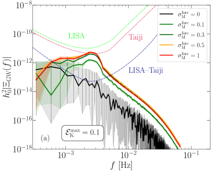
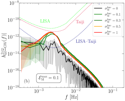
Figure 13: Similar to figure 12, helical GW spectrum $h_{0}^{2}|{\Xi}_{\rm GW}(f)|$ for signals produced at the EWPT from kinetically dominated (panel a), and magnetically dominated turbulence (panel b), using the results from the numerical simulations presented in ref. [65], shifted to ${\cal E}_{i}^{\rm max}=0.1$, with $i=$ M or K.

5 Conclusions

In the present work, we have studied the generation of polarized stochastic GW backgrounds produced by partially and fully helical turbulent sources, in particular, primordial magnetic fields. Our numerical simulations have confirmed that there is a direct correspondence between the magnetic helicity and the degree of circular polarization of the GWs produced from the resulting magnetic stress. We have calculated the GW spectra, both the energy density ${\Omega}_{\rm GW}(f)$ and the helicity ${\Xi}_{\rm GW}(f)$, that are produced by primordial magnetic fields for different values of the fractional magnetic helicity, and assuming two types of turbulence production. On the one hand, we have studied the production of GWs due to the presence of a fully developed turbulent magnetic field at the initial moment of GW production with a characteristic scale well defined by the turbulent process. On the other hand, we have studied the production of GWs due to a primordial magnetic field that is driven by an electromotive force that models magnetogenesis by injecting energy at a characteristic scale for a short duration (around a 10% of one Hubble time). In both cases, the resulting magnetic energy and helicity spectra are typical of fully developed turbulence, but their spectral shapes depend on the type of turbulence and the fractional helicity.

5.1 Numerical GW spectra

Our work confirms a shallow GW spectrum in the subinertial range that was obtained in previous numerical simulations [82]. We observe that the spectrum can instead possess even a small negative slope, instead of the flat spectrum reported in ref. [82], especially for low values of the helicity and for cases when the magnetic field is produced via turbulence forcing for a short duration; see figures 1–3. Such spectral slopes have also been reported in other recent numerical simulations which model the generation of magnetic fields via a forcing term [65, 99], and in ref. [116], in which the magnetic field is produced by the chiral magnetic effect. As suggested in ref. [99], this could be due to a finite size of the simulation domain or it could indeed be physical due to inverse transfer, analogous to that in helical [117] and non-helical hydromagnetic turbulence [118]. Additionally, it has been pointed out in refs. [98, 96] that the spectrum of the stress becomes shallower than white noise when the magnetic (or velocity) field is non-Gaussian, which would lead to a shallower GW spectrum. In the case when the magnetic field is driven, the MHD evolution might indeed generate a stochastic magnetic field with deviations from a Gaussian field. However, the exact shape of the GW spectrum at large scales requires further study.

5.2 GW polarization spectrum of magnetic fields initially present

In the runs with an initially given magnetic field, we show that the magnetic spectral shape does not depend on helicity, and the helicity spectrum has the same slopes as the magnetic spectrum, with a strength proportional to its fractional helicity (see figure 1). Both $E_{\rm M}(k)$ and $kH_{\rm M}(k)$ are characterized by a $k^{4}$ Batchelor spectrum below the peak at $k_{*}$ (taken to be $600$ in our simulations) and by a $k^{-5/3}$ Kolmogorov spectrum in the inertial range. The resulting GW spectrum $E_{\rm GW}(k)$ (defined per linear wave number interval) has an inertial range slope of $-11/3$, as was already shown in the numerical simulations of ref. [82], with a spectral peak at around $2k_{*}$, as expected, since GWs are sourced by the magnetic stress, which is obtained by convolution of the magnetic spectrum with itself. The helical GW spectrum $H_{\rm GW}(k)$ also has a similar spectral shape as the GW energy density spectrum. The exception is precisely at large scales (or low wave numbers), where we observe a decay of the helical GW spectrum in the smallest modes of the simulation (affecting the second and/or third largest wave numbers of the simulation). This becomes more noticeable for small values of the fractional magnetic helicity $|\sigma_{\rm M}|$. The reason for this is not clear, since this is not observed in the magnetic helicity spectrum, but it might be due to the finite size of the domain. In figure 5, we show that there are strong fluctuations at low wave numbers, which induce uncertainty on the actual value of the circular degree of polarization ${\cal P}_{\rm GW}(k)$ that is much reduced for larger wave numbers. In the case of an initial given magnetic field, the polarization degree follows the description given in refs. [62, 63, 64], after a few minor modifications, for turbulence dominated by helical transfer (HT), which assumes the same spectral slopes for the energy and helicity spectra, and relies on the assumptions of stationary turbulence and short sourcing; see figures 7 and 8. However, we showed that the polarization degree is not the same if computed directly from the strains, ${\cal P}_{h}(k)=A_{h}(k)/S_{h}(k)$, or from the time derivatives of the strains, ${\cal P}_{\rm GW}(k)=A_{\dot{h}}(k)/S_{\dot{h}}(k)=H_{\rm GW}(k)/E_{\rm GW}(k)$, the latter being the one that is in better agreement with the analytical description. We find a linear relation between the magnetic polarization degree ${\cal P}_{\rm M}$ and the resulting GW polarization ${\cal P}_{\rm GW}$, both obtained as the ratio of the total helicity of the magnetic or GW field to the total energy density; see figure 6. The linear relation ${\cal P}_{\rm GW}\sim{\cal P}_{\rm M}$, obtained from the numerical simulations, deviates from the analytical model considered in Appendix A; see figure 14. However, the model in Appendix A corresponds to a single-mode magnetic field of fractional magnetic helicity. Its generalization to a three-dimensional fully developed turbulent field is used for the numerical simulations; see equation (2.7).

5.3 GW polarization spectrum of magnetic fields initially driven

When the turbulence is forced for a finite duration, the situation changes drastically. Due to the quasi-monochromatic sourcing, a spike appears in the magnetic spectrum $E_{\rm M}(k)$ at initial times. When the magnetic energy density has reached its maximum value ${\cal E}_{\rm M}^{\rm max}$, and it starts to decay (which is taken to be at $t_{\rm max}=1.1$, given in Hubble times), the spike has smoothed around the spectral peak $k_{*}$ but it is still not completely gone; see figure 3. In the subinertial range, we observe a Batchelor spectrum with slopes very close to $4$, while in the inertial range, the spectrum has negative slopes, steeper than $-5/3$ (which corresponds to Kolmogorov turbulence). The spectrum of magnetic helicity $H_{\rm M}(k)$ presents a similar shape below and around the peak for all values of the fractional helicity above $|\sigma_{\rm M}|=0.3$ (shown in figure 3) with a fractional polarization of almost 1 in this range of wave numbers. The exception to this is for almost non-helical runs; see figure 2, for which the spectrum of helicity is negligible compared to the magnetic spectrum at all scales. At wave numbers above the peak, the helicity spectrum shows a sharper decrease with $k$ than the magnetic energy density, which becomes less pronounced as we increase the helicity, such that in the fully helical case the slopes of the magnetic and helicity spectra become very similar. This is plausibly explained by a forward cascade of current helicity [119]. The GW spectrum $E_{\rm GW}(k)$ shows a drop on amplitude at scales just below the peak that has also been observed in other recent numerical simulations [82, 99] due to the finite sourcing of the magnetic field. This drop appears also in the antisymmetric or helical spectrum of GWs $H_{\rm GW}(k)$, as we show in figure 3, and it does not depend on the fractional helicity. The GW degree of circular polarization ${\cal P}_{\rm GW}(k)$ in this case is shown in figure 5, where we show that it reaches the fully polarized case at the peak for large values of the fractional magnetic helicity $|\sigma_{\rm M}|$ and then decays at large wave numbers. The case with different slopes of the magnetic and helicity spectra was studied in previous analytical works [62, 63, 64], leading to a maximum degree of circular polarization of 80%, underpredicting it when compared to our numerical simulations. We compared in figure 9 the prediction of the polarization degree from the analytical model with our numerical results, showing that the numerical simulations do not follow the degree of circular polarization obtained by the analytical models in any of the two models considered previously, i.e., helical Kolmogorov (HK) or HT turbulence. Previous analytical assumptions were using a single power law for the magnetic energy and helicity spectra that did not depend on the wave number, besides the assumptions used to model the unequal time correlator and on the turbulence duration, as discussed in section 3.4. However, we showed in figures 8 and 9 that the predictions by the analytical models are more accurate, when compared to the numerical results, if we use the proper magnetic spectra obtained from the numerical simulations and evaluate the analytical model to compute the GW polarization degree using equations (3.2) and (3.3). This shows that the assumption of a single power law for the magnetic spectra affects more strongly the resulting polarization degree than the assumptions of short duration and stationary turbulence. We observe that in this case, the analytical model yields values of unity for the polarization degree at the peak, larger than those obtained in previous analytical estimations, and in agreement with the numerical simulations. Reference [65] studied the case of stationary turbulence, and computed the resulting GW degree of circular polarization. They also showed different values than previous analytical estimations for sources forced during larger times (around two Hubble times). It is unclear whether the discrepancies are due to the long duration of the forcing or due to the consideration of a single power law for the magnetic spectra. This aspect is left for future work. The precise form of the polarization degree can be important if one wants to infer the magnetic helicity from circular polarization measurements of GWs. Cosmological causal magnetic fields may well be close to fully helical because the magnetic helicity is a conserved quantity while the magnetic energy decays (and the correlation length increases), so the ratio always increases until it reaches nearly 100% if the magnetic field dynamically evolves for long enough, with a fractional helicity growth rate depending quadratically on its initial value: longer (shorter) period is needed for a field with smaller (higher) initial fractional magnetic helicity to become fully helical [120].

5.4 Detectability of the GW polarization with space-based GW detectors

Finally, we have explored the potential detectability of the GW signals by future space-based GW detectors if primordial partially or fully helical magnetic fields were present or produced at the EWPT. The resulting GW energy densities (shown in figure 11) are detectable by LISA with a SNR of 10 for magnetic energy densities of 10% of the radiation energy density if the magnetic field is initially given, and magnetic energy density ratios of at least 3% and 2% if the magnetic field is initially driven for a short (around 10% of the Hubble time) and a long duration (about two Hubble times), respectively. Even smaller magnetic amplitudes yield GW signals that can be detectable with second-generation space-based detectors, e.g., BBO and DECIGO. Using the dipole response induced by the proper motion of the solar system in the LISA interferometer channels, as recently studied in refs. [79, 64], a detectable polarized GW signal with a SNR of at least 10 requires magnetic energy densities above 10% of the radiation energy density (as shown in figures 12 and 13), which marginally coincides with the upper bound imposed by the BBN on the energy densities of additional relativistic components based on the abundance of light elements [121, 114, 115]. This is consistent with other turbulent sources; see, e.g., ref. [64], in which they require strong first-order phase transitions ($\alpha\sim 1$) to obtain a SNR of 10; see their figure 8. We can reach a maximum SNR of unity in the limit of 10% of energy density transformed in magnetic fields only in the case where the magnetic field is fully helical and forced for a long duration, following the numerical results of ref. [65]; see figure 13. Therefore, using the dipole response function of a planar space-based GW detector as LISA is not enough to detect the signals computed in the present work, although we highlight that our investigation is limited by the consideration of sub-relativistic velocities, which possibly leads to an underestimation of the signal strength [11]. In addition, following ref. [81], we have computed the power law sensitivity corresponding to a polarized GW signal by cross-correlating two space-based GW detectors, e.g., LISA and Taiji, which breaks the coplanarity of the detectors and allows one to detect polarization in the monopole response functions. We have shown that the GW degree of circular polarization produced by primordial magnetic fields generated at the EWPT can yield polarization SNR up to 20 if they are initially driven for a short time (about 10% of one Hubble time) with a maximum magnetic energy density of 10%, as long as the fractional magnetic helicity is $|\sigma_{\rm M}|\geq 0.3$ or, equivalently, $|{\cal P}_{\rm M}|\geq 0.5$; see figure 12. This is due to the fact that the resulting GW amplitudes are larger for smaller values of the fractional helicity; see figure 10, which compensates for the decrease in magnetic helicity. When the magnetic field is initially given, the polarization SNR of the GW signal stays approximately between 1 and 5, such that its potential detectability is more challenging.

Data availability

The source code used for the simulations of this study, the Pencil Code, is freely available [84]. The simulation data are also available at Ref. [122]. The calculations, the simulation data, and the routines generating the plots are also available on GitHub [123].

Appendix A Analytical model for polarization

We present in the current section the calculations of the GW spectra, both the symmetric $E_{\rm GW}(k)$ and the antisymmetric $H_{\rm GW}(k)$ functions, and the degree of circular polarization ${\cal P}_{\rm GW}(k)$, for a magnetic field with arbitrary fractional helicity that varies in one spatial direction, determined by the parameter $\sigma=\sigma_{\rm M}$. This model allows one to show analytically that fully helical magnetic fields induce circularly polarized GW signals, and to predict the dependence of the GW amplitude and polarization on the magnetic amplitude and fractional helicity. We start with a transverse magnetic field given as

$$\mathchoice{\mbox{\boldmath$\displaystyle B$}}{\mbox{\boldmath$\textstyle B$}}{\mbox{\boldmath$\scriptstyle B$}}{\mbox{\boldmath$\scriptscriptstyle B$}}{}(x,t)=\sqrt{\frac{2}{1+\sigma^{2}}}B_{0}\,\Theta(t-1)\left(\begin{array}[]{c}0\\ \sigma\sin k_{0}x\\ \cos k_{0}x\end{array}\right),$$ (A.1)

where $\sigma\in[0,1]$ is a parameter that modifies the helicity of the magnetic field, $k_{0}$ is the characteristic wave number, and ${\cal E}_{\rm M}={\textstyle{1\over 2}}\langle\mathchoice{\mbox{\boldmath$\displaystyle B$}}{\mbox{\boldmath$\textstyle B$}}{\mbox{\boldmath$\scriptstyle B$}}{\mbox{\boldmath$\scriptscriptstyle B$}}{}^{2}\rangle={\textstyle{1\over 2}}B_{0}^{2}$ is the magnetic energy density, with $B_{0}$ the magnetic field amplitude. The Heaviside function $\Theta(t-1)$ is included to indicate that this field is zero for $t\leq 1$. This field is a monochromatic 1D simplification of the general function used in the turbulence simulations; see equation (2.10). Note that when $\sigma=\pm 1$, we have a Beltrami (fully helical) field, that was studied in ref. [83] in the context of GW generation, and used to study numerical accuracy of the Pencil Code simulations. The vector potential $\textstyle A$ is defined such that $\mathchoice{\mbox{\boldmath$\displaystyle\nabla$}}{\mbox{\boldmath$\textstyle\nabla$}}{\mbox{\boldmath$\scriptstyle\nabla$}}{\mbox{\boldmath$\scriptscriptstyle\nabla$}}{}\times\mathchoice{\mbox{\boldmath$\displaystyle A$}}{\mbox{\boldmath$\textstyle A$}}{\mbox{\boldmath$\scriptstyle A$}}{\mbox{\boldmath$\scriptscriptstyle A$}}{}=\mathchoice{\mbox{\boldmath$\displaystyle B$}}{\mbox{\boldmath$\textstyle B$}}{\mbox{\boldmath$\scriptstyle B$}}{\mbox{\boldmath$\scriptscriptstyle B$}}{}$,

$$\mathchoice{\mbox{\boldmath$\displaystyle A$}}{\mbox{\boldmath$\textstyle A$}}{\mbox{\boldmath$\scriptstyle A$}}{\mbox{\boldmath$\scriptscriptstyle A$}}{}(x,t)=\sqrt{\frac{2}{1+\sigma^{2}}}\frac{B_{0}}{k_{0}}\,\Theta(t-1)\left(\begin{array}[]{c}0\\ \sin k_{0}x\\ \sigma\cos k_{0}x\end{array}\right)+\mathchoice{\mbox{\boldmath$\displaystyle A$}}{\mbox{\boldmath$\textstyle A$}}{\mbox{\boldmath$\scriptstyle A$}}{\mbox{\boldmath$\scriptscriptstyle A$}}{}_{g},$$ (A.2)

where $\mathchoice{\mbox{\boldmath$\displaystyle A$}}{\mbox{\boldmath$\textstyle A$}}{\mbox{\boldmath$\scriptstyle A$}}{\mbox{\boldmath$\scriptscriptstyle A$}}{}_{g}$ is gauge-dependent, and the helicity of the magnetic field is

$${\cal H}_{\rm M}=\langle\mathchoice{\mbox{\boldmath$\displaystyle B$}}{\mbox{\boldmath$\textstyle B$}}{\mbox{\boldmath$\scriptstyle B$}}{\mbox{\boldmath$\scriptscriptstyle B$}}{}\cdot\mathchoice{\mbox{\boldmath$\displaystyle A$}}{\mbox{\boldmath$\textstyle A$}}{\mbox{\boldmath$\scriptstyle A$}}{\mbox{\boldmath$\scriptscriptstyle A$}}{}\rangle=\frac{2\sigma}{1+\sigma^{2}}\frac{B_{0}^{2}}{k_{0}},$$ (A.3)

which is not gauge-dependent. The magnetic energy density $E_{\rm M}(k)$ and the helicity $H_{\rm M}(k)$ spectra are

$$E_{\rm M}(k,t)= \,{\textstyle{1\over 2}}\int_{\Omega_{1}}\mathchoice{\mbox{\boldmath$\displaystyle\tilde{B}$}}{\mbox{\boldmath$\textstyle\tilde{B}$}}{\mbox{\boldmath$\scriptstyle\tilde{B}$}}{\mbox{\boldmath$\scriptscriptstyle\tilde{B}$}}{}(\mathchoice{\mbox{\boldmath$\displaystyle k$}}{\mbox{\boldmath$\textstyle k$}}{\mbox{\boldmath$\scriptstyle k$}}{\mbox{\boldmath$\scriptscriptstyle k$}}{},t)\cdot\mathchoice{\mbox{\boldmath$\displaystyle\tilde{B}$}}{\mbox{\boldmath$\textstyle\tilde{B}$}}{\mbox{\boldmath$\scriptstyle\tilde{B}$}}{\mbox{\boldmath$\scriptscriptstyle\tilde{B}$}}{}^{*}(\mathchoice{\mbox{\boldmath$\displaystyle k$}}{\mbox{\boldmath$\textstyle k$}}{\mbox{\boldmath$\scriptstyle k$}}{\mbox{\boldmath$\scriptscriptstyle k$}}{},t)\,{\rm d}{}\Omega_{1}={\cal E}_{\rm M}\,\Theta(t-1)\,\delta(k-|k_{0}|),$$ (A.4)

$$H_{\rm M}(k,t)= \,\int_{\Omega_{1}}\mathchoice{\mbox{\boldmath$\displaystyle\tilde{B}$}}{\mbox{\boldmath$\textstyle\tilde{B}$}}{\mbox{\boldmath$\scriptstyle\tilde{B}$}}{\mbox{\boldmath$\scriptscriptstyle\tilde{B}$}}{}(\mathchoice{\mbox{\boldmath$\displaystyle k$}}{\mbox{\boldmath$\textstyle k$}}{\mbox{\boldmath$\scriptstyle k$}}{\mbox{\boldmath$\scriptscriptstyle k$}}{},t)\cdot\mathchoice{\mbox{\boldmath$\displaystyle\tilde{A}$}}{\mbox{\boldmath$\textstyle\tilde{A}$}}{\mbox{\boldmath$\scriptstyle\tilde{A}$}}{\mbox{\boldmath$\scriptscriptstyle\tilde{A}$}}{}^{*}(\mathchoice{\mbox{\boldmath$\displaystyle k$}}{\mbox{\boldmath$\textstyle k$}}{\mbox{\boldmath$\scriptstyle k$}}{\mbox{\boldmath$\scriptscriptstyle k$}}{},t){\rm d}{}\Omega_{1}=\frac{2\sigma}{1+\sigma^{2}}\frac{2{\cal E}_{\rm M}}{k_{0}}\,\Theta(t-1)|k_{0}|\,\delta(k-|k_{0}|),$$ (A.5)

where $\Omega_{1}=2$ is the one-dimensional solid angle and $\delta(k)$ is the one-dimensional Dirac’s delta function. The fractional magnetic helicity is

$${\cal P}_{\rm M}=\frac{k_{0}\langle\mathchoice{\mbox{\boldmath$\displaystyle B$}}{\mbox{\boldmath$\textstyle B$}}{\mbox{\boldmath$\scriptstyle B$}}{\mbox{\boldmath$\scriptscriptstyle B$}}{}(x,t)\cdot\mathchoice{\mbox{\boldmath$\displaystyle A$}}{\mbox{\boldmath$\textstyle A$}}{\mbox{\boldmath$\scriptstyle A$}}{\mbox{\boldmath$\scriptscriptstyle A$}}{}(x,t)\rangle}{\langle\mathchoice{\mbox{\boldmath$\displaystyle B$}}{\mbox{\boldmath$\textstyle B$}}{\mbox{\boldmath$\scriptstyle B$}}{\mbox{\boldmath$\scriptscriptstyle B$}}{}^{2}(x,t)\rangle}=\frac{k_{0}{\cal H}_{\rm M}}{2{\cal E}_{\rm M}}=\frac{2\sigma}{1+\sigma^{2}},$$ (A.6)

which reduces to $+1$, $0$, and $-1$, for $\sigma=+1$, $0$, and $-1$, respectively. The stress tensor of the magnetic fields is

$$T_{ij}(x,t)=-B_{i}B_{j}+\frac{1}{2}\delta_{ij}\mathchoice{\mbox{\boldmath$\displaystyle B$}}{\mbox{\boldmath$\textstyle B$}}{\mbox{\boldmath$\scriptstyle B$}}{\mbox{\boldmath$\scriptscriptstyle B$}}{}^{2},$$ (A.7)

with

$$\mathchoice{\mbox{\boldmath$\displaystyle B$}}{\mbox{\boldmath$\textstyle B$}}{\mbox{\boldmath$\scriptstyle B$}}{\mbox{\boldmath$\scriptscriptstyle B$}}{}^{2}(x,t)=2{\cal E}_{\rm M}\,\Theta(t-1)\left(1+\frac{1-\sigma^{2}}{1+\sigma^{2}}\cos 2k_{0}x\right),$$ (A.8)

and

$$-B_{i}B_{j}(x,t)=-\frac{2{\cal E}_{\rm M}}{1+\sigma^{2}}\,\Theta(t-1)\left(\begin{array}[]{c c c}0&0&0\\ 0&\sigma^{2}(1-\cos 2k_{0}x)&\sigma\sin 2k_{0}x\\ 0&\sigma\sin 2k_{0}x&1+\cos 2k_{0}x\end{array}\right).$$ (A.9)

Combining equations (A.8) and (A.9), we obtain the stress tensor

$$T_{ij}(x,t)={\cal E}_{\rm M}\,\Theta(t-1)\left(\begin{array}[]{c c c}T_{11}(x)&0&0\\ 0&T_{22}(x)&T_{12}(x)\\ 0&T_{12}(x)&-T_{22}(x)\end{array}\right),$$ (A.10)

with

$$T_{11}(x)= \,1+\frac{1-\sigma^{2}}{1+\sigma^{2}}\cos 2k_{0}x,$$

$$T_{22}(x)= \,1+\frac{1-\sigma^{2}}{1+\sigma^{2}}\cos 2k_{0}x-\frac{2\sigma^{2}}{1+\sigma^{2}}(1-\cos 2k_{0}x)=\frac{1-\sigma^{2}}{1+\sigma^{2}}+\cos 2k_{0}x,$$

$$T_{12}(x)= \,-\frac{2\sigma}{1+\sigma^{2}}\sin 2k_{0}x,$$ (A.11)

which becomes $T_{11}(x)=1$, $T_{22}(x)=\cos 2k_{0}x$, and $T_{12}(x)=\mp\sin 2k_{0}x$ in the fully helical case (i.e., $\sigma=\pm 1$) studied in ref. [83]. Since GWs are produced by linear perturbations over the metric tensor, and the stress tensor components are also perturbations over background fields, constant modes ($\mathchoice{\mbox{\boldmath$\displaystyle k$}}{\mbox{\boldmath$\textstyle k$}}{\mbox{\boldmath$\scriptstyle k$}}{\mbox{\boldmath$\scriptscriptstyle k$}}{}={\bf 0}$) do not produce GWs. For this reason, we can neglect the terms that are homogeneous in space, and we write

$$T_{ij}^{\rm TT}(x,t)=\frac{{\cal E}_{\rm M}}{1+\sigma^{2}}\,\Theta(t-1)\left(\begin{array}[]{c c c}0&0&0\\ 0&(1+\sigma^{2})\cos 2k_{0}x&-2\sigma\sin 2k_{0}x\\ 0&-2\sigma\sin 2k_{0}x&-(1+\sigma^{2})\cos 2k_{0}x\end{array}\right),$$ (A.12)

where we noted that taking $T_{11}$ to zero, the stress tensor becomes traceless and transverse (TT), with the $+$ and $\times$ modes,

$$T_{+}(x,t)={\cal E}_{\rm M}\,\Theta(t-1)\cos 2k_{0}x,\quad T_{\times}(x,t)={\cal E}_{\rm M}{\cal P}_{\rm M}\,\Theta(t-1)\sin 2k_{0}x,$$ (A.13)

where we have used ${\cal P}_{\rm M}$, given in equation (A.6). In Fourier space, the resulting stress tensor components are

$$\tilde{T}_{+}(k_{x}=\pm 2k_{0},t)={\textstyle{1\over 2}}{\cal E}_{\rm M}\,\Theta(t-1),\quad\tilde{T}_{\times}(k_{x}=\pm 2k_{0},t)=\mp{\textstyle{1\over 2}}i{\cal E}_{\rm M}{\cal P}_{\rm M}\,\Theta(t-1).$$ (A.14)

The GW strains $\tilde{h}_{+}(k_{x},t)$ and $\tilde{h}_{\times}(k_{x},t)$ are computed from the GW equation (2.2) with initial condition $h_{+,\times}=\partial_{t}h_{+,\times}=0$ at $t=1$, and assuming flat non-expanding space-time for the radiation-dominated epoch (see ref. [83] for more details),

$$\tilde{h}_{+}(\pm 2k_{0},t)= \,\frac{3}{k_{0}}\int_{1}^{t}\tilde{T}_{+}(\pm 2k_{0},\tau)\sin[2k_{0}(t-\tau)]\,{\rm d}{}\tau=\frac{3}{4k_{0}^{2}}{\cal E}_{\rm M}\,\Theta(t-1)\left(1-\cos[2k_{0}(t-1)]\right)$$

$$= \,\frac{3}{2k_{0}^{2}}{\cal E}_{\rm M}\sin^{2}[k_{0}(t-1)]\,\Theta(t-1),$$ (A.15)

$$\tilde{h}_{\times}(\pm 2k_{0},t)= \,\frac{3}{k_{0}}\int_{1}^{t}\tilde{T}_{\times}(\pm 2k_{0},\tau)\sin[2k_{0}(t-\tau)]\,{\rm d}{}\tau$$

$$= \,\mp\frac{3i}{2k_{0}^{2}}{\cal P}_{\rm M}{\cal E}_{\rm M}\sin^{2}[k_{0}(t-1)]\,\Theta(t-1).$$ (A.16)

The spectral functions $S_{h}(k,t)$ and $A_{h}(k,t)$ are

$$S_{h}(2|k_{0}|,t)= \,\int_{\Omega_{1}}\left[\tilde{h}_{+}(\mathchoice{\mbox{\boldmath$\displaystyle k$}}{\mbox{\boldmath$\textstyle k$}}{\mbox{\boldmath$\scriptstyle k$}}{\mbox{\boldmath$\scriptscriptstyle k$}}{},t)\tilde{h}_{+}^{*}(\mathchoice{\mbox{\boldmath$\displaystyle k$}}{\mbox{\boldmath$\textstyle k$}}{\mbox{\boldmath$\scriptstyle k$}}{\mbox{\boldmath$\scriptscriptstyle k$}}{},t)+\tilde{h}_{\times}(\mathchoice{\mbox{\boldmath$\displaystyle k$}}{\mbox{\boldmath$\textstyle k$}}{\mbox{\boldmath$\scriptstyle k$}}{\mbox{\boldmath$\scriptscriptstyle k$}}{},t)\tilde{h}_{\times}^{*}(\mathchoice{\mbox{\boldmath$\displaystyle k$}}{\mbox{\boldmath$\textstyle k$}}{\mbox{\boldmath$\scriptstyle k$}}{\mbox{\boldmath$\scriptscriptstyle k$}}{},t)\right]{\rm d}{}\Omega_{\mathchoice{\mbox{\boldmath$\displaystyle k$}}{\mbox{\boldmath$\textstyle k$}}{\mbox{\boldmath$\scriptstyle k$}}{\mbox{\boldmath$\scriptscriptstyle k$}}{}}$$

$$= \,\frac{9}{2k_{0}^{4}}\left(1+{\cal P}_{\rm M}^{2}\right){\cal E}_{\rm M}^{2}\sin^{4}[k_{0}(t-1)]\,\Theta(t-1),$$ (A.17)

$$iA_{h}(2|k_{0}|,t)= \,\int_{\Omega_{1}}\left[\tilde{h}_{+}(\mathchoice{\mbox{\boldmath$\displaystyle k$}}{\mbox{\boldmath$\textstyle k$}}{\mbox{\boldmath$\scriptstyle k$}}{\mbox{\boldmath$\scriptscriptstyle k$}}{},t)\tilde{h}_{\times}^{*}(\mathchoice{\mbox{\boldmath$\displaystyle k$}}{\mbox{\boldmath$\textstyle k$}}{\mbox{\boldmath$\scriptstyle k$}}{\mbox{\boldmath$\scriptscriptstyle k$}}{},t)-\tilde{h}_{+}^{*}(\mathchoice{\mbox{\boldmath$\displaystyle k$}}{\mbox{\boldmath$\textstyle k$}}{\mbox{\boldmath$\scriptstyle k$}}{\mbox{\boldmath$\scriptscriptstyle k$}}{},t)\tilde{h}_{\times}(\mathchoice{\mbox{\boldmath$\displaystyle k$}}{\mbox{\boldmath$\textstyle k$}}{\mbox{\boldmath$\scriptstyle k$}}{\mbox{\boldmath$\scriptscriptstyle k$}}{},t)\right]{\rm d}{}\Omega_{\mathchoice{\mbox{\boldmath$\displaystyle k$}}{\mbox{\boldmath$\textstyle k$}}{\mbox{\boldmath$\scriptstyle k$}}{\mbox{\boldmath$\scriptscriptstyle k$}}{}}$$

$$= \,i\frac{9}{k_{0}^{4}}{\cal P}_{\rm M}{\cal E}_{\rm M}^{2}\sin^{4}[k_{0}(t-1)]\,\Theta(t-1),$$ (A.18)

and zero for all the other values of the wave number $k$. The spectrum of the characteristic amplitude $h_{\rm c}(k,t)$, and its total value integrated over $k$, are

$$h_{\rm c}(2|k_{0}|,t)= \,\sqrt{kS_{h}(k,t)}$$

$$= \,\frac{3}{k_{0}^{2}}\sqrt{|k_{0}|\left(1+{\cal P}_{\rm M}^{2}\right)}{\cal E}_{\rm M}\sin^{2}[k_{0}(t-1)]\,\Theta(t-1),$$ (A.19)

$$h_{\rm c}(t)= \,\left(\int S_{h}(k,t)\,{\rm d}{}k\right)^{1/2}$$

$$= \,\frac{3}{k_{0}^{2}}\sqrt{{\textstyle{1\over 2}}\left(1+{\cal P}_{\rm M}^{2}\right)}{\cal E}_{\rm M}\sin^{2}[k_{0}(t-1)]\,\Theta(t-1).$$ (A.20)

The characteristic amplitude averaged over oscillations in time is $h_{\rm c}={\textstyle{3\over 2}}\sqrt{{\textstyle{1\over 2}}(1+{\cal P}_{\rm M}^{2})}{\cal E}_{\rm M}/k_{0}^{2}$, and the polarization ${\cal P}_{h}$ is

$${\cal P}_{h}=\frac{A_{h}(2|k_{0}|,t)}{S_{h}(2|k_{0}|,t)}=\frac{2{\cal P}_{\rm M}}{1+{\cal P}_{\rm M}^{2}}.$$ (A.21)

The spectral functions $S_{\dot{h}}(k,t)$ and $A_{\dot{h}}(k,t)$ are

$$S_{\dot{h}}(2|k_{0}|,t)= \,\int_{\Omega_{1}}\left[\tilde{\dot{h}}_{+}(\mathchoice{\mbox{\boldmath$\displaystyle k$}}{\mbox{\boldmath$\textstyle k$}}{\mbox{\boldmath$\scriptstyle k$}}{\mbox{\boldmath$\scriptscriptstyle k$}}{},t)\tilde{\dot{h}}_{+}^{*}(\mathchoice{\mbox{\boldmath$\displaystyle k$}}{\mbox{\boldmath$\textstyle k$}}{\mbox{\boldmath$\scriptstyle k$}}{\mbox{\boldmath$\scriptscriptstyle k$}}{},t)+\tilde{\dot{h}}_{\times}(\mathchoice{\mbox{\boldmath$\displaystyle k$}}{\mbox{\boldmath$\textstyle k$}}{\mbox{\boldmath$\scriptstyle k$}}{\mbox{\boldmath$\scriptscriptstyle k$}}{},t)\tilde{\dot{h}}_{\times}^{*}(\mathchoice{\mbox{\boldmath$\displaystyle k$}}{\mbox{\boldmath$\textstyle k$}}{\mbox{\boldmath$\scriptstyle k$}}{\mbox{\boldmath$\scriptscriptstyle k$}}{},t)\right]{\rm d}{}\Omega_{\mathchoice{\mbox{\boldmath$\displaystyle k$}}{\mbox{\boldmath$\textstyle k$}}{\mbox{\boldmath$\scriptstyle k$}}{\mbox{\boldmath$\scriptscriptstyle k$}}{}}$$

$$= \,\frac{9}{2k_{0}^{2}}\left(1+{\cal P}_{\rm M}^{2}\right){\cal E}_{\rm M}^{2}\sin^{2}[2k_{0}(t-1)]\,\Theta(t-1),$$ (A.22)

$$iA_{\dot{h}}(2|k_{0}|,t)= \,\int_{\Omega_{1}}\left[\tilde{\dot{h}}_{+}(\mathchoice{\mbox{\boldmath$\displaystyle k$}}{\mbox{\boldmath$\textstyle k$}}{\mbox{\boldmath$\scriptstyle k$}}{\mbox{\boldmath$\scriptscriptstyle k$}}{},t)\tilde{\dot{h}}_{\times}^{*}(\mathchoice{\mbox{\boldmath$\displaystyle k$}}{\mbox{\boldmath$\textstyle k$}}{\mbox{\boldmath$\scriptstyle k$}}{\mbox{\boldmath$\scriptscriptstyle k$}}{},t)-\tilde{\dot{h}}_{+}^{*}(\mathchoice{\mbox{\boldmath$\displaystyle k$}}{\mbox{\boldmath$\textstyle k$}}{\mbox{\boldmath$\scriptstyle k$}}{\mbox{\boldmath$\scriptscriptstyle k$}}{},t)\tilde{\dot{h}}_{\times}(\mathchoice{\mbox{\boldmath$\displaystyle k$}}{\mbox{\boldmath$\textstyle k$}}{\mbox{\boldmath$\scriptstyle k$}}{\mbox{\boldmath$\scriptscriptstyle k$}}{},t)\right]{\rm d}{}\Omega_{\mathchoice{\mbox{\boldmath$\displaystyle k$}}{\mbox{\boldmath$\textstyle k$}}{\mbox{\boldmath$\scriptstyle k$}}{\mbox{\boldmath$\scriptscriptstyle k$}}{}}$$

$$= \,i\frac{9}{k_{0}^{2}}{\cal P}_{\rm M}{\cal E}_{\rm M}^{2}\sin^{2}[2k_{0}(t-1)]\,\Theta(t-1),$$ (A.23)

such that ${\cal P}_{\rm GW}=A_{\dot{h}}(k,t)/S_{\dot{h}}(k,t)=A_{h}(k,t)/S_{h}(k,t)={\cal P}_{h}$; see equation (A.21). The GW spectrum ${\Omega}_{\rm GW}(k,t)$ and the total GW energy density are

$${\Omega}_{\rm GW}(2|k_{0}|,t)=\frac{kS_{\dot{h}}(k,t)}{6}= \,\frac{3}{2|k_{0}|}\left(1+{\cal P}_{\rm M}^{2}\right){\cal E}_{\rm M}^{2}\sin^{2}[2k_{0}(t-1)]\,\Theta(t-1),$$ (A.24)

$${\Omega}_{\rm GW}(t)=\frac{1}{6}\int_{0}^{\infty}S_{\dot{h}}(k,t)\,{\rm d}{}k= \,\frac{3}{4k_{0}^{2}}\left(1+{\cal P}_{\rm M}^{2}\right){\cal E}_{\rm M}^{2}\sin^{2}[2k_{0}(t-1)]\,\Theta(t-1).$$ (A.25)

The GW energy density averaged over oscillations in time is ${\Omega}_{\rm GW}={\textstyle{3\over 8}}(1+{\cal P}_{\rm M}^{2}){\cal E}_{\rm M}^{2}/k_{0}^{2}$. The energy ratio is ${\Omega}_{\rm GW}/{\cal E}_{\rm M}={\textstyle{1\over 2}}h_{\rm c}\,\sqrt{{\textstyle{1\over 2}}(1+{\cal P}_{\rm M}^{2})}$, which was reported in ref. [83] for the fully helical field, i.e., ${\cal P}_{\rm M}=\pm 1$. For larger (smaller) values of the fractional magnetic helicity $|{\cal P}_{\rm M}|$, this result predicts larger (smaller) amplitudes of the GW energy density by a factor $1+{\cal P}_{\rm M}^{2}\in[1,2]$; see figure 14. In turbulent simulations; see figure 10, we observe that ${\Omega}_{\rm GW}$ is not noticeably dependent on ${\cal P}_{\rm M}$ if the magnetic field is initially given, and that it decreases for larger values of $|{\cal P}_{\rm M}|$ if the magnetic field is initially driven.

We find that the symmetric functions $S_{h}(k,t)$ and $S_{\dot{h}}(k,t)$, and hence the characteristic amplitude $h_{\rm c}(k,t)$ and the GW energy density ${\Omega}_{\rm GW}(k,t)$, are proportional to the function ${\textstyle{1\over 2}}(1+{\cal P}_{\rm M}^{2})$, while the antisymmetric functions $A_{h}(k,t)$ and $A_{\dot{h}}(k,t)$, are proportional to ${\cal P}_{\rm M}$. These functions and the degree of circular polarization are shown in figure 14 compared to the empirical relation ${\cal P}_{\rm GW}\approx{\cal P}_{\rm M}=2\sigma_{\rm M}/(1+\sigma_{\rm M}^{2})$, obtained from the numerical simulations; see figure 6.

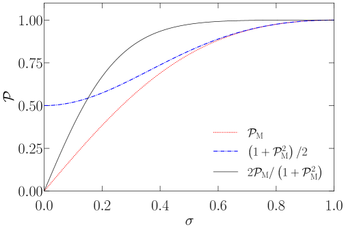
Figure 14: Functions ${\textstyle{1\over 2}}(1+{\cal P}_{\rm M}^{2})$ and ${\cal P}_{\rm M}$, that appear in the symmetric and antisymmetric functions of the GW spectra, respectively, and degree of circular polarization ${\cal P}_{\rm GW}=2{\cal P}_{\rm M}/(1+{\cal P}_{\rm M}^{2})$ obtained for the 1D analytical model. We obtained the numerical fit ${\cal P}_{\rm GW}\sim{\cal P}_{\rm M}$ in the numerical simulations of MHD turbulence; see figure 6.

Appendix B LISA and Taiji interferometry

B.1 Time-delay interferometry

We derive here some of the expressions that are useful to compute the response functions and sensitivity curves of LISA and Taiji. Both space-based GW detectors have triangular configurations with three arms of the same length, $L=2.5\times 10^{6}\,{\rm km}$ for LISA [7], and $L=3\times 10^{6}\,{\rm km}$ for Taiji [124]. The combination of two arms with a common mass at their vertices is a Michelson interferometer. Hence, the 3 arms of LISA or Taiji lead to three interferometers that correspond to the physical channels $X$, $Y$, and $Z$. These channels are linearly combined to obtain the time-delay interferometry (TDI) channels of LISA, commonly known as $A$, $E$, and $T$ [125], and we call $C$, $D$, and $S$, the analogous Taiji channels, as done in ref. [81]. Following ref. [79], the time delay $\delta t$ induced by a gravitational wave in each of the detector arms is

$$\sigma_{i}=\frac{c\delta t}{2L}=\sum_{\lambda=+,-}\int\tilde{h}_{\lambda}(\mathchoice{\mbox{\boldmath$\displaystyle k$}}{\mbox{\boldmath$\textstyle k$}}{\mbox{\boldmath$\scriptstyle k$}}{\mbox{\boldmath$\scriptscriptstyle k$}}{},t-L/c)\,e_{ab}^{\lambda}(\hat{\mathchoice{\mbox{\boldmath$\displaystyle k$}}{\mbox{\boldmath$\textstyle k$}}{\mbox{\boldmath$\scriptstyle k$}}{\mbox{\boldmath$\scriptscriptstyle k$}}}{}){\cal Q}_{i}^{ab}(\mathchoice{\mbox{\boldmath$\displaystyle k$}}{\mbox{\boldmath$\textstyle k$}}{\mbox{\boldmath$\scriptstyle k$}}{\mbox{\boldmath$\scriptscriptstyle k$}}{}),$$ (B.1)

where $+$ and $-$ are the helical polarization modes, $e_{ab}^{\pm}(\hat{\mathchoice{\mbox{\boldmath$\displaystyle k$}}{\mbox{\boldmath$\textstyle k$}}{\mbox{\boldmath$\scriptstyle k$}}{\mbox{\boldmath$\scriptscriptstyle k$}}}{})$ are the helical polarization basis tensors, $i$ indicates each of the interferometers $i=1$, $2$, $3$, and ${\cal Q}_{i}^{ab}(\mathchoice{\mbox{\boldmath$\displaystyle k$}}{\mbox{\boldmath$\textstyle k$}}{\mbox{\boldmath$\scriptstyle k$}}{\mbox{\boldmath$\scriptscriptstyle k$}}{})$ are the interferometer response functions,

$${\cal Q}_{1}^{ab}(\mathchoice{\mbox{\boldmath$\displaystyle k$}}{\mbox{\boldmath$\textstyle k$}}{\mbox{\boldmath$\scriptstyle k$}}{\mbox{\boldmath$\scriptscriptstyle k$}}{})=e^{-ikL\hat{\mathchoice{\mbox{\boldmath$\displaystyle k$}}{\mbox{\boldmath$\textstyle k$}}{\mbox{\boldmath$\scriptstyle k$}}{\mbox{\boldmath$\scriptscriptstyle k$}}}{}\cdot\hat{\mathchoice{\mbox{\boldmath$\displaystyle x$}}{\mbox{\boldmath$\textstyle x$}}{\mbox{\boldmath$\scriptstyle x$}}{\mbox{\boldmath$\scriptscriptstyle x$}}}{}_{1}}\left[{\cal T}(kL,\hat{\mathchoice{\mbox{\boldmath$\displaystyle k$}}{\mbox{\boldmath$\textstyle k$}}{\mbox{\boldmath$\scriptstyle k$}}{\mbox{\boldmath$\scriptscriptstyle k$}}}{}\cdot\hat{\mathchoice{\mbox{\boldmath$\displaystyle U$}}{\mbox{\boldmath$\textstyle U$}}{\mbox{\boldmath$\scriptstyle U$}}{\mbox{\boldmath$\scriptscriptstyle U$}}}{}_{1})\,\hat{\mathchoice{\mbox{\boldmath$\displaystyle U$}}{\mbox{\boldmath$\textstyle U$}}{\mbox{\boldmath$\scriptstyle U$}}{\mbox{\boldmath$\scriptscriptstyle U$}}}{}_{1}^{a}\hat{\mathchoice{\mbox{\boldmath$\displaystyle U$}}{\mbox{\boldmath$\textstyle U$}}{\mbox{\boldmath$\scriptstyle U$}}{\mbox{\boldmath$\scriptscriptstyle U$}}}{}_{1}^{b}-{\cal T}(kL,-\hat{\mathchoice{\mbox{\boldmath$\displaystyle k$}}{\mbox{\boldmath$\textstyle k$}}{\mbox{\boldmath$\scriptstyle k$}}{\mbox{\boldmath$\scriptscriptstyle k$}}}{}\cdot\hat{\mathchoice{\mbox{\boldmath$\displaystyle U$}}{\mbox{\boldmath$\textstyle U$}}{\mbox{\boldmath$\scriptstyle U$}}{\mbox{\boldmath$\scriptscriptstyle U$}}}{}_{3})\,\hat{\mathchoice{\mbox{\boldmath$\displaystyle U$}}{\mbox{\boldmath$\textstyle U$}}{\mbox{\boldmath$\scriptstyle U$}}{\mbox{\boldmath$\scriptscriptstyle U$}}}{}_{3}^{a}\hat{\mathchoice{\mbox{\boldmath$\displaystyle U$}}{\mbox{\boldmath$\textstyle U$}}{\mbox{\boldmath$\scriptstyle U$}}{\mbox{\boldmath$\scriptscriptstyle U$}}}{}_{3}^{b}\right],$$

$${\cal Q}_{2}^{ab}(\mathchoice{\mbox{\boldmath$\displaystyle k$}}{\mbox{\boldmath$\textstyle k$}}{\mbox{\boldmath$\scriptstyle k$}}{\mbox{\boldmath$\scriptscriptstyle k$}}{})=e^{-ikL\hat{\mathchoice{\mbox{\boldmath$\displaystyle k$}}{\mbox{\boldmath$\textstyle k$}}{\mbox{\boldmath$\scriptstyle k$}}{\mbox{\boldmath$\scriptscriptstyle k$}}}{}\cdot\hat{\mathchoice{\mbox{\boldmath$\displaystyle x$}}{\mbox{\boldmath$\textstyle x$}}{\mbox{\boldmath$\scriptstyle x$}}{\mbox{\boldmath$\scriptscriptstyle x$}}}{}_{2}}\left[{\cal T}(kL,\hat{\mathchoice{\mbox{\boldmath$\displaystyle k$}}{\mbox{\boldmath$\textstyle k$}}{\mbox{\boldmath$\scriptstyle k$}}{\mbox{\boldmath$\scriptscriptstyle k$}}}{}\cdot\hat{\mathchoice{\mbox{\boldmath$\displaystyle U$}}{\mbox{\boldmath$\textstyle U$}}{\mbox{\boldmath$\scriptstyle U$}}{\mbox{\boldmath$\scriptscriptstyle U$}}}{}_{2})\,\hat{\mathchoice{\mbox{\boldmath$\displaystyle U$}}{\mbox{\boldmath$\textstyle U$}}{\mbox{\boldmath$\scriptstyle U$}}{\mbox{\boldmath$\scriptscriptstyle U$}}}{}_{2}^{a}\hat{\mathchoice{\mbox{\boldmath$\displaystyle U$}}{\mbox{\boldmath$\textstyle U$}}{\mbox{\boldmath$\scriptstyle U$}}{\mbox{\boldmath$\scriptscriptstyle U$}}}{}_{2}^{b}-{\cal T}(kL,-\hat{\mathchoice{\mbox{\boldmath$\displaystyle k$}}{\mbox{\boldmath$\textstyle k$}}{\mbox{\boldmath$\scriptstyle k$}}{\mbox{\boldmath$\scriptscriptstyle k$}}}{}\cdot\hat{\mathchoice{\mbox{\boldmath$\displaystyle U$}}{\mbox{\boldmath$\textstyle U$}}{\mbox{\boldmath$\scriptstyle U$}}{\mbox{\boldmath$\scriptscriptstyle U$}}}{}_{1})\,\hat{\mathchoice{\mbox{\boldmath$\displaystyle U$}}{\mbox{\boldmath$\textstyle U$}}{\mbox{\boldmath$\scriptstyle U$}}{\mbox{\boldmath$\scriptscriptstyle U$}}}{}_{1}^{a}\hat{\mathchoice{\mbox{\boldmath$\displaystyle U$}}{\mbox{\boldmath$\textstyle U$}}{\mbox{\boldmath$\scriptstyle U$}}{\mbox{\boldmath$\scriptscriptstyle U$}}}{}_{1}^{b}\right],$$

$${\cal Q}_{3}^{ab}(\mathchoice{\mbox{\boldmath$\displaystyle k$}}{\mbox{\boldmath$\textstyle k$}}{\mbox{\boldmath$\scriptstyle k$}}{\mbox{\boldmath$\scriptscriptstyle k$}}{})=e^{-ikL\hat{\mathchoice{\mbox{\boldmath$\displaystyle k$}}{\mbox{\boldmath$\textstyle k$}}{\mbox{\boldmath$\scriptstyle k$}}{\mbox{\boldmath$\scriptscriptstyle k$}}}{}\cdot\hat{\mathchoice{\mbox{\boldmath$\displaystyle x$}}{\mbox{\boldmath$\textstyle x$}}{\mbox{\boldmath$\scriptstyle x$}}{\mbox{\boldmath$\scriptscriptstyle x$}}}{}_{3}}\left[{\cal T}(kL,\hat{\mathchoice{\mbox{\boldmath$\displaystyle k$}}{\mbox{\boldmath$\textstyle k$}}{\mbox{\boldmath$\scriptstyle k$}}{\mbox{\boldmath$\scriptscriptstyle k$}}}{}\cdot\hat{\mathchoice{\mbox{\boldmath$\displaystyle U$}}{\mbox{\boldmath$\textstyle U$}}{\mbox{\boldmath$\scriptstyle U$}}{\mbox{\boldmath$\scriptscriptstyle U$}}}{}_{3})\,\hat{\mathchoice{\mbox{\boldmath$\displaystyle U$}}{\mbox{\boldmath$\textstyle U$}}{\mbox{\boldmath$\scriptstyle U$}}{\mbox{\boldmath$\scriptscriptstyle U$}}}{}_{3}^{a}\hat{\mathchoice{\mbox{\boldmath$\displaystyle U$}}{\mbox{\boldmath$\textstyle U$}}{\mbox{\boldmath$\scriptstyle U$}}{\mbox{\boldmath$\scriptscriptstyle U$}}}{}_{3}^{b}-{\cal T}(kL,-\hat{\mathchoice{\mbox{\boldmath$\displaystyle k$}}{\mbox{\boldmath$\textstyle k$}}{\mbox{\boldmath$\scriptstyle k$}}{\mbox{\boldmath$\scriptscriptstyle k$}}}{}\cdot\hat{\mathchoice{\mbox{\boldmath$\displaystyle U$}}{\mbox{\boldmath$\textstyle U$}}{\mbox{\boldmath$\scriptstyle U$}}{\mbox{\boldmath$\scriptscriptstyle U$}}}{}_{2})\,\hat{\mathchoice{\mbox{\boldmath$\displaystyle U$}}{\mbox{\boldmath$\textstyle U$}}{\mbox{\boldmath$\scriptstyle U$}}{\mbox{\boldmath$\scriptscriptstyle U$}}}{}_{2}^{a}\hat{\mathchoice{\mbox{\boldmath$\displaystyle U$}}{\mbox{\boldmath$\textstyle U$}}{\mbox{\boldmath$\scriptstyle U$}}{\mbox{\boldmath$\scriptscriptstyle U$}}}{}_{2}^{b}\right],$$ (B.2)

with $\cal T$ being the $i$-th detector transfer function,

$${\cal T}(kL,\hat{\mathchoice{\mbox{\boldmath$\displaystyle k$}}{\mbox{\boldmath$\textstyle k$}}{\mbox{\boldmath$\scriptstyle k$}}{\mbox{\boldmath$\scriptscriptstyle k$}}}{}\cdot\hat{\mathchoice{\mbox{\boldmath$\displaystyle U$}}{\mbox{\boldmath$\textstyle U$}}{\mbox{\boldmath$\scriptstyle U$}}{\mbox{\boldmath$\scriptscriptstyle U$}}}{}_{i})= \,e^{-{\textstyle{1\over 2}}ikL(1+\hat{\mathchoice{\mbox{\boldmath$\displaystyle k$}}{\mbox{\boldmath$\textstyle k$}}{\mbox{\boldmath$\scriptstyle k$}}{\mbox{\boldmath$\scriptscriptstyle k$}}}{}\cdot\hat{\mathchoice{\mbox{\boldmath$\displaystyle U$}}{\mbox{\boldmath$\textstyle U$}}{\mbox{\boldmath$\scriptstyle U$}}{\mbox{\boldmath$\scriptscriptstyle U$}}}{}_{i})}\,{\rm sinc}\left[{\textstyle{1\over 2}}kL(1-\hat{\mathchoice{\mbox{\boldmath$\displaystyle k$}}{\mbox{\boldmath$\textstyle k$}}{\mbox{\boldmath$\scriptstyle k$}}{\mbox{\boldmath$\scriptscriptstyle k$}}}{}\cdot\hat{\mathchoice{\mbox{\boldmath$\displaystyle U$}}{\mbox{\boldmath$\textstyle U$}}{\mbox{\boldmath$\scriptstyle U$}}{\mbox{\boldmath$\scriptscriptstyle U$}}}{}_{i})\right]$$

$$+ \,e^{+{\textstyle{1\over 2}}ikL(1-\hat{\mathchoice{\mbox{\boldmath$\displaystyle k$}}{\mbox{\boldmath$\textstyle k$}}{\mbox{\boldmath$\scriptstyle k$}}{\mbox{\boldmath$\scriptscriptstyle k$}}}{}\cdot\hat{\mathchoice{\mbox{\boldmath$\displaystyle U$}}{\mbox{\boldmath$\textstyle U$}}{\mbox{\boldmath$\scriptstyle U$}}{\mbox{\boldmath$\scriptscriptstyle U$}}}{}_{i})}\,{\rm sinc}\left[{\textstyle{1\over 2}}kL(1+\hat{\mathchoice{\mbox{\boldmath$\displaystyle k$}}{\mbox{\boldmath$\textstyle k$}}{\mbox{\boldmath$\scriptstyle k$}}{\mbox{\boldmath$\scriptscriptstyle k$}}}{}\cdot\hat{\mathchoice{\mbox{\boldmath$\displaystyle U$}}{\mbox{\boldmath$\textstyle U$}}{\mbox{\boldmath$\scriptstyle U$}}{\mbox{\boldmath$\scriptscriptstyle U$}}}{}_{i})\right],$$ (B.3)

where ${\rm sinc}(x)=\sin(x)/x$. The vectors $\hat{\mathchoice{\mbox{\boldmath$\displaystyle U$}}{\mbox{\boldmath$\textstyle U$}}{\mbox{\boldmath$\scriptstyle U$}}{\mbox{\boldmath$\scriptscriptstyle U$}}}{}_{i}$ are the unit vectors following the direction of the arms, i.e., the vector pointing from spacecraft $i$ to $i+1$ (modulo 3), with $i=1$, $2$, $3$. We can define a reference frame in which the interferometer is located in the $xz$-plane, with the three spacecraft located at $\mathchoice{\mbox{\boldmath$\displaystyle x$}}{\mbox{\boldmath$\textstyle x$}}{\mbox{\boldmath$\scriptstyle x$}}{\mbox{\boldmath$\scriptscriptstyle x$}}{}_{1}=(0,0,0)$, $\mathchoice{\mbox{\boldmath$\displaystyle x$}}{\mbox{\boldmath$\textstyle x$}}{\mbox{\boldmath$\scriptstyle x$}}{\mbox{\boldmath$\scriptscriptstyle x$}}{}_{2}=L(0,0,1)$, and $\mathchoice{\mbox{\boldmath$\displaystyle x$}}{\mbox{\boldmath$\textstyle x$}}{\mbox{\boldmath$\scriptstyle x$}}{\mbox{\boldmath$\scriptscriptstyle x$}}{}_{3}={\textstyle{1\over 2}}L(\sqrt{3},0,1)$, chosen for simplicity. It can be shown that rotations of the plane do not affect the response function after integrating over all directions in the sky [126]. Hence, the unit vectors along the arms are

$$\hat{\mathchoice{\mbox{\boldmath$\displaystyle U$}}{\mbox{\boldmath$\textstyle U$}}{\mbox{\boldmath$\scriptstyle U$}}{\mbox{\boldmath$\scriptscriptstyle U$}}}{}_{1} \,=\hat{\mathchoice{\mbox{\boldmath$\displaystyle x$}}{\mbox{\boldmath$\textstyle x$}}{\mbox{\boldmath$\scriptstyle x$}}{\mbox{\boldmath$\scriptscriptstyle x$}}}{}_{2}-\hat{\mathchoice{\mbox{\boldmath$\displaystyle x$}}{\mbox{\boldmath$\textstyle x$}}{\mbox{\boldmath$\scriptstyle x$}}{\mbox{\boldmath$\scriptscriptstyle x$}}}{}_{1}=(0,0,1),$$

$$\hat{\mathchoice{\mbox{\boldmath$\displaystyle U$}}{\mbox{\boldmath$\textstyle U$}}{\mbox{\boldmath$\scriptstyle U$}}{\mbox{\boldmath$\scriptscriptstyle U$}}}{}_{2} \,=\hat{\mathchoice{\mbox{\boldmath$\displaystyle x$}}{\mbox{\boldmath$\textstyle x$}}{\mbox{\boldmath$\scriptstyle x$}}{\mbox{\boldmath$\scriptscriptstyle x$}}}{}_{3}-\hat{\mathchoice{\mbox{\boldmath$\displaystyle x$}}{\mbox{\boldmath$\textstyle x$}}{\mbox{\boldmath$\scriptstyle x$}}{\mbox{\boldmath$\scriptscriptstyle x$}}}{}_{2}={\textstyle{1\over 2}}(\sqrt{3},0,-1),$$

$$\hat{\mathchoice{\mbox{\boldmath$\displaystyle U$}}{\mbox{\boldmath$\textstyle U$}}{\mbox{\boldmath$\scriptstyle U$}}{\mbox{\boldmath$\scriptscriptstyle U$}}}{}_{3} \,=\hat{\mathchoice{\mbox{\boldmath$\displaystyle x$}}{\mbox{\boldmath$\textstyle x$}}{\mbox{\boldmath$\scriptstyle x$}}{\mbox{\boldmath$\scriptscriptstyle x$}}}{}_{1}-\hat{\mathchoice{\mbox{\boldmath$\displaystyle x$}}{\mbox{\boldmath$\textstyle x$}}{\mbox{\boldmath$\scriptstyle x$}}{\mbox{\boldmath$\scriptscriptstyle x$}}}{}_{3}=-{\textstyle{1\over 2}}(\sqrt{3},0,1).$$ (B.4)

We describe the wave vectors in spherical coordinates,

$$\mathchoice{\mbox{\boldmath$\displaystyle k$}}{\mbox{\boldmath$\textstyle k$}}{\mbox{\boldmath$\scriptstyle k$}}{\mbox{\boldmath$\scriptscriptstyle k$}}{}=k(\cos\phi\sin\theta,\sin\phi\sin\theta,\cos\theta),$$ (B.5)

with $\phi\in[0,2\pi]$ and $\theta\in[0,\pi]$, such that the terms $\hat{\mathchoice{\mbox{\boldmath$\displaystyle k$}}{\mbox{\boldmath$\textstyle k$}}{\mbox{\boldmath$\scriptstyle k$}}{\mbox{\boldmath$\scriptscriptstyle k$}}}{}\cdot\hat{\mathchoice{\mbox{\boldmath$\displaystyle x$}}{\mbox{\boldmath$\textstyle x$}}{\mbox{\boldmath$\scriptstyle x$}}{\mbox{\boldmath$\scriptscriptstyle x$}}}{}_{i}$ that appear in the response functions ${\cal Q}_{i}^{ab}(\mathchoice{\mbox{\boldmath$\displaystyle k$}}{\mbox{\boldmath$\textstyle k$}}{\mbox{\boldmath$\scriptstyle k$}}{\mbox{\boldmath$\scriptscriptstyle k$}}{})$; see equation (B.2), are

$$\hat{\mathchoice{\mbox{\boldmath$\displaystyle k$}}{\mbox{\boldmath$\textstyle k$}}{\mbox{\boldmath$\scriptstyle k$}}{\mbox{\boldmath$\scriptscriptstyle k$}}}{}\cdot\hat{\mathchoice{\mbox{\boldmath$\displaystyle x$}}{\mbox{\boldmath$\textstyle x$}}{\mbox{\boldmath$\scriptstyle x$}}{\mbox{\boldmath$\scriptscriptstyle x$}}}{}_{1}=0,\quad\hat{\mathchoice{\mbox{\boldmath$\displaystyle k$}}{\mbox{\boldmath$\textstyle k$}}{\mbox{\boldmath$\scriptstyle k$}}{\mbox{\boldmath$\scriptscriptstyle k$}}}{}\cdot\hat{\mathchoice{\mbox{\boldmath$\displaystyle x$}}{\mbox{\boldmath$\textstyle x$}}{\mbox{\boldmath$\scriptstyle x$}}{\mbox{\boldmath$\scriptscriptstyle x$}}}{}_{2}=\cos\theta,\quad\hat{\mathchoice{\mbox{\boldmath$\displaystyle k$}}{\mbox{\boldmath$\textstyle k$}}{\mbox{\boldmath$\scriptstyle k$}}{\mbox{\boldmath$\scriptscriptstyle k$}}}{}\cdot\hat{\mathchoice{\mbox{\boldmath$\displaystyle x$}}{\mbox{\boldmath$\textstyle x$}}{\mbox{\boldmath$\scriptstyle x$}}{\mbox{\boldmath$\scriptscriptstyle x$}}}{}_{3}={\textstyle{1\over 2}}\left(\sqrt{3}\cos\phi\sin\theta+\cos\theta\right),$$ (B.6)

and the products $\hat{\mathchoice{\mbox{\boldmath$\displaystyle k$}}{\mbox{\boldmath$\textstyle k$}}{\mbox{\boldmath$\scriptstyle k$}}{\mbox{\boldmath$\scriptscriptstyle k$}}}{}\cdot\hat{\mathchoice{\mbox{\boldmath$\displaystyle U$}}{\mbox{\boldmath$\textstyle U$}}{\mbox{\boldmath$\scriptstyle U$}}{\mbox{\boldmath$\scriptscriptstyle U$}}}{}_{i}$ that appear in the interferometer transfer functions $\cal T$; see equation (B.3), are

$$\hat{\mathchoice{\mbox{\boldmath$\displaystyle k$}}{\mbox{\boldmath$\textstyle k$}}{\mbox{\boldmath$\scriptstyle k$}}{\mbox{\boldmath$\scriptscriptstyle k$}}}{}\cdot\hat{\mathchoice{\mbox{\boldmath$\displaystyle U$}}{\mbox{\boldmath$\textstyle U$}}{\mbox{\boldmath$\scriptstyle U$}}{\mbox{\boldmath$\scriptscriptstyle U$}}}{}_{1}= \,\cos\theta,$$

$$\hat{\mathchoice{\mbox{\boldmath$\displaystyle k$}}{\mbox{\boldmath$\textstyle k$}}{\mbox{\boldmath$\scriptstyle k$}}{\mbox{\boldmath$\scriptscriptstyle k$}}}{}\cdot\hat{\mathchoice{\mbox{\boldmath$\displaystyle U$}}{\mbox{\boldmath$\textstyle U$}}{\mbox{\boldmath$\scriptstyle U$}}{\mbox{\boldmath$\scriptscriptstyle U$}}}{}_{2}= \,{\textstyle{1\over 2}}\left(\sqrt{3}\cos\phi\sin\theta-\cos\theta\right),$$

$$\hat{\mathchoice{\mbox{\boldmath$\displaystyle k$}}{\mbox{\boldmath$\textstyle k$}}{\mbox{\boldmath$\scriptstyle k$}}{\mbox{\boldmath$\scriptscriptstyle k$}}}{}\cdot\hat{\mathchoice{\mbox{\boldmath$\displaystyle U$}}{\mbox{\boldmath$\textstyle U$}}{\mbox{\boldmath$\scriptstyle U$}}{\mbox{\boldmath$\scriptscriptstyle U$}}}{}_{3}= \,-{\textstyle{1\over 2}}\left(\sqrt{3}\cos\phi\sin\theta+\cos\theta\right).$$ (B.7)

The signals of the channels $A$, $E$, and $T$  are obtained by linearly combining the $X$, $Y$, and $Z$ interferometer channels (or $i=1$, $2$, $3$, in equation (B.1)),

$$\Sigma_{A}=\frac{1}{3}\left(2\sigma_{X}-\sigma_{Y}-\sigma_{Z}\right),\quad\Sigma_{E}=\frac{1}{\sqrt{3}}\left(\sigma_{Z}-\sigma_{Y}\right),\quad\Sigma_{T}=\frac{1}{3}\left(\sigma_{X}+\sigma_{Y}+\sigma_{Z}\right).$$ (B.8)

Combining (B.1) and (B.8), we can define ${\cal Q}_{O}^{ab}(\mathchoice{\mbox{\boldmath$\displaystyle k$}}{\mbox{\boldmath$\textstyle k$}}{\mbox{\boldmath$\scriptstyle k$}}{\mbox{\boldmath$\scriptscriptstyle k$}}{})$ as a function of ${\cal Q}_{i}^{ab}(\mathchoice{\mbox{\boldmath$\displaystyle k$}}{\mbox{\boldmath$\textstyle k$}}{\mbox{\boldmath$\scriptstyle k$}}{\mbox{\boldmath$\scriptscriptstyle k$}}{})$,

$${\cal Q}_{O}^{ab}(\mathchoice{\mbox{\boldmath$\displaystyle k$}}{\mbox{\boldmath$\textstyle k$}}{\mbox{\boldmath$\scriptstyle k$}}{\mbox{\boldmath$\scriptscriptstyle k$}}{})=\frac{1}{3}\left(\begin{array}[]{ccc}2&-1&-1\\ 0&-\sqrt{3}&\sqrt{3}\\ 1&1&1\end{array}\right){\cal Q}_{i}^{ab}(\mathchoice{\mbox{\boldmath$\displaystyle k$}}{\mbox{\boldmath$\textstyle k$}}{\mbox{\boldmath$\scriptstyle k$}}{\mbox{\boldmath$\scriptscriptstyle k$}}{}),$$ (B.9)

where $O=A$, $E$, and $T$.

B.2 Signal and response functions

The two-point correlation function of the signals that a stochastic GW background produces in the time domain in two of the channels, $O$ and $O^{\prime}$, can be expanded as a function of the peculiar velocity of the solar system, $v/c=1.23\times 10^{-3}$ [79],

$$\langle\Sigma_{O}(t)\Sigma_{O^{\prime}}(t^{\prime})\rangle= \,\frac{1}{8}\sum_{\lambda=+,-}\int{\rm d}{}k\Biggl{[}{\cal M}_{OO^{\prime}}^{\lambda}(k)S_{h}^{\lambda}(k)\cos\left[ck(t-t^{\prime})\right]$$

$$+\frac{v}{c}{\cal D}_{OO^{\prime}}^{\lambda}(k,\hat{\mathchoice{\mbox{\boldmath$\displaystyle v$}}{\mbox{\boldmath$\textstyle v$}}{\mbox{\boldmath$\scriptstyle v$}}{\mbox{\boldmath$\scriptscriptstyle v$}}}{})\left(S_{h}^{\lambda}(k)-k\frac{{\rm d}{}S_{h}^{\lambda}(k)}{{\rm d}{}k}\right)\sin\left[ck(t-t^{\prime})\right]+{\cal O}\left(\frac{v^{2}}{c^{2}}\right)\Biggr{]},$$ (B.10)

where the strain spectral functions $S_{h}^{\pm}(k)$  are defined using the $+$ and $-$ polarization basis, such that $S_{h}(k)=S_{h}^{+}(k)+S_{h}^{-}(k)$ and $A_{h}(k)=S_{h}^{+}(k)-S_{h}^{-}(k)$. ${\cal M}_{OO^{\prime}}^{\pm}(k)$ and ${\cal D}_{OO^{\prime}}^{\pm}(k,\hat{\mathchoice{\mbox{\boldmath$\displaystyle v$}}{\mbox{\boldmath$\textstyle v$}}{\mbox{\boldmath$\scriptstyle v$}}{\mbox{\boldmath$\scriptscriptstyle v$}}}{})$ are the monopole and dipole quadratic interferometer response functions of the channels $O$ and $O^{\prime}$,

$${\cal M}_{OO^{\prime}}^{\pm}(k)= \,4\int\frac{{\rm d}{}\Omega_{k}}{4\pi}e_{ab}^{\pm}(\hat{\mathchoice{\mbox{\boldmath$\displaystyle k$}}{\mbox{\boldmath$\textstyle k$}}{\mbox{\boldmath$\scriptstyle k$}}{\mbox{\boldmath$\scriptscriptstyle k$}}}{})e_{cd}^{\pm}(-\hat{\mathchoice{\mbox{\boldmath$\displaystyle k$}}{\mbox{\boldmath$\textstyle k$}}{\mbox{\boldmath$\scriptstyle k$}}{\mbox{\boldmath$\scriptscriptstyle k$}}}{}){\cal Q}_{O}^{ab}(\mathchoice{\mbox{\boldmath$\displaystyle k$}}{\mbox{\boldmath$\textstyle k$}}{\mbox{\boldmath$\scriptstyle k$}}{\mbox{\boldmath$\scriptscriptstyle k$}}{}){\cal Q}_{O^{\prime}}^{cd}(-\mathchoice{\mbox{\boldmath$\displaystyle k$}}{\mbox{\boldmath$\textstyle k$}}{\mbox{\boldmath$\scriptstyle k$}}{\mbox{\boldmath$\scriptscriptstyle k$}}{}),$$ (B.11)

$${\cal D}_{OO^{\prime}}^{\pm}(k,\hat{\mathchoice{\mbox{\boldmath$\displaystyle v$}}{\mbox{\boldmath$\textstyle v$}}{\mbox{\boldmath$\scriptstyle v$}}{\mbox{\boldmath$\scriptscriptstyle v$}}}{})= \,4i\int\frac{{\rm d}{}\Omega_{k}}{4\pi}e_{ab}^{\pm}(\hat{\mathchoice{\mbox{\boldmath$\displaystyle k$}}{\mbox{\boldmath$\textstyle k$}}{\mbox{\boldmath$\scriptstyle k$}}{\mbox{\boldmath$\scriptscriptstyle k$}}}{})e_{cd}^{\pm}(-\hat{\mathchoice{\mbox{\boldmath$\displaystyle k$}}{\mbox{\boldmath$\textstyle k$}}{\mbox{\boldmath$\scriptstyle k$}}{\mbox{\boldmath$\scriptscriptstyle k$}}}{}){\cal Q}_{O}^{ab}(\mathchoice{\mbox{\boldmath$\displaystyle k$}}{\mbox{\boldmath$\textstyle k$}}{\mbox{\boldmath$\scriptstyle k$}}{\mbox{\boldmath$\scriptscriptstyle k$}}{}){\cal Q}_{O^{\prime}}^{cd}(-\mathchoice{\mbox{\boldmath$\displaystyle k$}}{\mbox{\boldmath$\textstyle k$}}{\mbox{\boldmath$\scriptstyle k$}}{\mbox{\boldmath$\scriptscriptstyle k$}}{})\,\hat{\mathchoice{\mbox{\boldmath$\displaystyle k$}}{\mbox{\boldmath$\textstyle k$}}{\mbox{\boldmath$\scriptstyle k$}}{\mbox{\boldmath$\scriptscriptstyle k$}}}{}\cdot\hat{\mathchoice{\mbox{\boldmath$\displaystyle v$}}{\mbox{\boldmath$\textstyle v$}}{\mbox{\boldmath$\scriptstyle v$}}{\mbox{\boldmath$\scriptscriptstyle v$}}}{},$$ (B.12)

where $\hat{\mathchoice{\mbox{\boldmath$\displaystyle v$}}{\mbox{\boldmath$\textstyle v$}}{\mbox{\boldmath$\scriptstyle v$}}{\mbox{\boldmath$\scriptscriptstyle v$}}}{}$ is the unit direction of the peculiar velocity, and the wave number is $ck=2\pi f$ due to the GW dispersion relation, such that we can express the response functions in terms of $f$. The dipole response function appears due to the anisotropies induced by the proper motion of the solar system. It depends on the angle $\alpha$ between the orientation of the detector plane and the peculiar velocity of the solar system. Expressing $\textstyle k$ in spherical coordinates, see equation (B.5), we can perform the integral over the directions on the sky,

$${\cal M}_{OO^{\prime}}^{\pm}(k)=\frac{1}{\pi}\int_{0}^{2\pi}{\rm d}{}\phi\int_{0}^{\pi}e_{ab}^{\pm}(\hat{\mathchoice{\mbox{\boldmath$\displaystyle k$}}{\mbox{\boldmath$\textstyle k$}}{\mbox{\boldmath$\scriptstyle k$}}{\mbox{\boldmath$\scriptscriptstyle k$}}}{})e_{cd}^{\pm}(-\hat{\mathchoice{\mbox{\boldmath$\displaystyle k$}}{\mbox{\boldmath$\textstyle k$}}{\mbox{\boldmath$\scriptstyle k$}}{\mbox{\boldmath$\scriptscriptstyle k$}}}{}){\cal Q}_{O}^{ab}(\mathchoice{\mbox{\boldmath$\displaystyle k$}}{\mbox{\boldmath$\textstyle k$}}{\mbox{\boldmath$\scriptstyle k$}}{\mbox{\boldmath$\scriptscriptstyle k$}}{}){\cal Q}_{O^{\prime}}^{cd,*}(\mathchoice{\mbox{\boldmath$\displaystyle k$}}{\mbox{\boldmath$\textstyle k$}}{\mbox{\boldmath$\scriptstyle k$}}{\mbox{\boldmath$\scriptscriptstyle k$}}{})\sin\theta\,{\rm d}{}\theta,$$ (B.13)

where we have used ${\cal Q}_{O^{\prime}}^{cd}(-\mathchoice{\mbox{\boldmath$\displaystyle k$}}{\mbox{\boldmath$\textstyle k$}}{\mbox{\boldmath$\scriptstyle k$}}{\mbox{\boldmath$\scriptscriptstyle k$}}{})={\cal Q}_{O^{\prime}}^{cd,*}(\mathchoice{\mbox{\boldmath$\displaystyle k$}}{\mbox{\boldmath$\textstyle k$}}{\mbox{\boldmath$\scriptstyle k$}}{\mbox{\boldmath$\scriptscriptstyle k$}}{})$ [126]. The product $e_{ab}^{\pm}(\hat{\mathchoice{\mbox{\boldmath$\displaystyle k$}}{\mbox{\boldmath$\textstyle k$}}{\mbox{\boldmath$\scriptstyle k$}}{\mbox{\boldmath$\scriptscriptstyle k$}}}{})e_{cd}^{\pm}(-\hat{\mathchoice{\mbox{\boldmath$\displaystyle k$}}{\mbox{\boldmath$\textstyle k$}}{\mbox{\boldmath$\scriptstyle k$}}{\mbox{\boldmath$\scriptscriptstyle k$}}}{})$ can be written as [79]

$$e_{ab}^{\pm}(\hat{\mathchoice{\mbox{\boldmath$\displaystyle k$}}{\mbox{\boldmath$\textstyle k$}}{\mbox{\boldmath$\scriptstyle k$}}{\mbox{\boldmath$\scriptscriptstyle k$}}}{})e_{cd}^{\pm}(-\hat{\mathchoice{\mbox{\boldmath$\displaystyle k$}}{\mbox{\boldmath$\textstyle k$}}{\mbox{\boldmath$\scriptstyle k$}}{\mbox{\boldmath$\scriptscriptstyle k$}}}{})=\frac{1}{4}\left(\delta_{ac}-\hat{k}_{a}\hat{k}_{c}\mp i\varepsilon_{ace}\hat{k}^{e}\right)\left(\delta_{bd}-\hat{k}_{b}\hat{k}_{d}\mp i\varepsilon_{bde}\hat{k}^{e}\right),$$ (B.14)

where $\delta_{ab}$ is the Kronecker delta and $\varepsilon_{abc}$ is the Levi-Civita tensor. It can be shown that ${\cal M}_{OO^{\prime}}^{+}(f)={\cal M}_{OO^{\prime}}^{-}(f)$, so the monopole responses to the $+$ and $-$ modes are the same, and hence, polarization of the GW signals cannot be detected unless we consider the dipole response or combine more than one GW detector to break the coplanarity, as we do in Appendix B.4. The responses of the LISA channels $A$ and $E$ are the same, i.e., ${\cal M}_{EE}(f)={\cal M}_{AA}(f)$, and ${\cal M}_{TT}(f)$ is much smaller in the low frequency regime, being insensitive to gravitational wave signals. For this reason, the $T$ channel is known as the “Sagnac” or null channel and it is used to identify and subtract noisy signals [125]. The response of the combined $A$ and $E$ channels is ${\cal M}_{AE}(f)=0$ [79]. Note that ${\cal M}_{AA}(f)$ corresponds to the LISA geometrical factor $\tilde{\cal R}^{A}(f)$, commonly defined in the LISA community; see, e.g., refs. [127, 110, 128, 81], which can be well-fit for LISA and Taiji by

$$\tilde{\cal R}(f)=\frac{3}{10}\left[1+0.6\left(2\pi fL/c\right)^{2}\right]^{-1}.$$ (B.15)

The monopole and dipole response functions of LISA and Taiji are shown in figure 15.

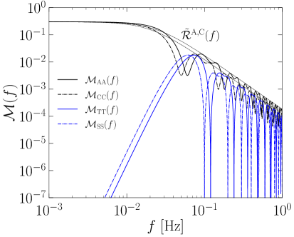
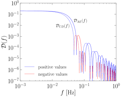
Figure 15: Monopole response functions (left panel) of the LISA $A$ and $E$ channels, ${\cal M}_{\rm AA}(f)$, the Taiji $C$ and $D$ channels, ${\cal M}_{CC}(f)$, and the LISA $T$ and Taiji $S$ null channels, ${\cal M}_{TT}(f)$ and ${\cal M}_{SS}(f)$ respectively, compared with the analytical fit of the LISA and Taiji geometric function $\tilde{\cal R}^{A,C}(f)$. Dipole response functions (right panel) induced by the peculiar velocity of the solar system in the LISA correlated $A$ and $E$ channels, ${\cal D}_{AE}(f)$, and the Taiji $C$ and $D$ channels, ${\cal D}_{CD}(f)$.

The dipole response function can be expressed as a function of the angle $\alpha$ between the normal of the detector and the velocity of the proper motion $\hat{\mathchoice{\mbox{\boldmath$\displaystyle v$}}{\mbox{\boldmath$\textstyle v$}}{\mbox{\boldmath$\scriptstyle v$}}{\mbox{\boldmath$\scriptscriptstyle v$}}}{}$. Since we integrate over all directions of $\hat{\mathchoice{\mbox{\boldmath$\displaystyle k$}}{\mbox{\boldmath$\textstyle k$}}{\mbox{\boldmath$\scriptstyle k$}}{\mbox{\boldmath$\scriptscriptstyle k$}}}{}$ in the sky, we can define the vector $\textstyle v$ in the frame of reference in which we have defined the detector (in the $xz$-plane), such that the normal $\hat{\mathchoice{\mbox{\boldmath$\displaystyle n$}}{\mbox{\boldmath$\textstyle n$}}{\mbox{\boldmath$\scriptstyle n$}}{\mbox{\boldmath$\scriptscriptstyle n$}}}{}$ is in the $y$-direction, and due to the symmetry of the integration over $\hat{\mathchoice{\mbox{\boldmath$\displaystyle k$}}{\mbox{\boldmath$\textstyle k$}}{\mbox{\boldmath$\scriptstyle k$}}{\mbox{\boldmath$\scriptscriptstyle k$}}}{}$, we can neglect the projection of $\textstyle v$ on the detector plane, and write $\mathchoice{\mbox{\boldmath$\displaystyle v$}}{\mbox{\boldmath$\textstyle v$}}{\mbox{\boldmath$\scriptstyle v$}}{\mbox{\boldmath$\scriptscriptstyle v$}}{}=v(0,\cos\alpha,0)$, or $\hat{\mathchoice{\mbox{\boldmath$\displaystyle k$}}{\mbox{\boldmath$\textstyle k$}}{\mbox{\boldmath$\scriptstyle k$}}{\mbox{\boldmath$\scriptscriptstyle k$}}}{}\cdot\hat{\mathchoice{\mbox{\boldmath$\displaystyle v$}}{\mbox{\boldmath$\textstyle v$}}{\mbox{\boldmath$\scriptstyle v$}}{\mbox{\boldmath$\scriptscriptstyle v$}}}{}=\cos\alpha\sin\phi\sin\theta$. This allows us to compute ${\cal D}_{OO^{\prime}}^{\pm}(k,\alpha)$ as a function of the angle $\alpha$ [79],

$${\cal D}_{OO^{\prime}}^{\pm}(k,\alpha)=\frac{i}{\pi}\cos\alpha\int_{0}^{2\pi}\sin\phi\,{\rm d}{}\phi\int_{0}^{\pi}e_{ab}^{\pm}(\hat{\mathchoice{\mbox{\boldmath$\displaystyle k$}}{\mbox{\boldmath$\textstyle k$}}{\mbox{\boldmath$\scriptstyle k$}}{\mbox{\boldmath$\scriptscriptstyle k$}}}{})e_{cd}^{\pm}(-\hat{\mathchoice{\mbox{\boldmath$\displaystyle k$}}{\mbox{\boldmath$\textstyle k$}}{\mbox{\boldmath$\scriptstyle k$}}{\mbox{\boldmath$\scriptscriptstyle k$}}}{}){\cal Q}_{O}^{ab}(\mathchoice{\mbox{\boldmath$\displaystyle k$}}{\mbox{\boldmath$\textstyle k$}}{\mbox{\boldmath$\scriptstyle k$}}{\mbox{\boldmath$\scriptscriptstyle k$}}{}){\cal Q}_{O^{\prime}}^{cd,*}(\mathchoice{\mbox{\boldmath$\displaystyle k$}}{\mbox{\boldmath$\textstyle k$}}{\mbox{\boldmath$\scriptstyle k$}}{\mbox{\boldmath$\scriptscriptstyle k$}}{})\sin^{2}\theta\,{\rm d}{}\theta.$$ (B.16)

It can be shown that ${\cal D}_{OO^{\prime}}^{+}(k,\alpha)=-{\cal D}_{OO^{\prime}}^{-}(k,\alpha)$ for $O$, $O^{\prime}=A$, $E$, $T$, and ${\cal D}_{AA}^{\pm}(k,\alpha)={\cal D}_{EE}^{\pm}(k,\alpha)=0$ [79]. Hence, the relevant contributions from the dipole response function are ${\cal D}_{AE}^{+}(k,\alpha)={\cal D}_{EA}^{+}(k,\alpha)=-{\cal D}_{AE}^{-}(k,\alpha)=-{\cal D}_{EA}^{-}(k,\alpha)$, and we can write ${\cal D}_{AE}^{\pm}(k,\alpha)=\pm{\cal D}_{AE}(k)\cos\alpha$.

At the present time $t_{0}$, the observed GW energy density, defined in equation (2.14), by the detector is [94]

$${\Omega}_{\rm GW}(t_{0})= \,\frac{1}{12H_{0}^{2}}\langle\dot{h}_{ij}^{\rm phys}(\mathchoice{\mbox{\boldmath$\displaystyle x$}}{\mbox{\boldmath$\textstyle x$}}{\mbox{\boldmath$\scriptstyle x$}}{\mbox{\boldmath$\scriptscriptstyle x$}}{},t)\dot{h}_{ij}^{\rm phys}(\mathchoice{\mbox{\boldmath$\displaystyle x$}}{\mbox{\boldmath$\textstyle x$}}{\mbox{\boldmath$\scriptstyle x$}}{\mbox{\boldmath$\scriptscriptstyle x$}}{},t)\rangle=\frac{\pi^{2}f^{2}}{3H_{0}^{2}}\langle h_{ij}^{\rm phys}(\mathchoice{\mbox{\boldmath$\displaystyle x$}}{\mbox{\boldmath$\textstyle x$}}{\mbox{\boldmath$\scriptstyle x$}}{\mbox{\boldmath$\scriptscriptstyle x$}}{},t)h_{ij}^{\rm phys}(\mathchoice{\mbox{\boldmath$\displaystyle x$}}{\mbox{\boldmath$\textstyle x$}}{\mbox{\boldmath$\scriptstyle x$}}{\mbox{\boldmath$\scriptscriptstyle x$}}{},t)\rangle$$

$$= \,\frac{2\pi^{2}f^{2}}{3H_{0}^{2}}\langle h_{+}^{2}(\mathchoice{\mbox{\boldmath$\displaystyle x$}}{\mbox{\boldmath$\textstyle x$}}{\mbox{\boldmath$\scriptstyle x$}}{\mbox{\boldmath$\scriptscriptstyle x$}}{},t)+h_{-}^{2}(\mathchoice{\mbox{\boldmath$\displaystyle x$}}{\mbox{\boldmath$\textstyle x$}}{\mbox{\boldmath$\scriptstyle x$}}{\mbox{\boldmath$\scriptscriptstyle x$}}{},t)\rangle,$$ (B.17)

where $H_{0}=100\,h_{0}\,{\rm km}\,{\rm s}^{-1}\,{\rm Mpc}^{-1}$ and $h_{0}$ takes into account the uncertainties of the Hubble rate at the present time [94]. We have used the relation $\langle\dot{h}_{ij}^{\rm phys}\dot{h}_{ij}^{\rm phys}\rangle=c^{2}k^{2}\langle h_{ij}^{\rm phys}h_{ij}^{\rm phys}\rangle$ and the GW dispersion relation $ck=2\pi f$. The resulting GW spectrum ${\Omega}_{\rm GW}(f)={\Omega}_{\rm GW}^{+}(f)+{\Omega}_{\rm GW}^{-}(f)$ is

$${\Omega}_{\rm GW}^{\pm}(f)=\frac{2\pi^{2}f^{3}}{3H_{0}^{2}}S_{h}^{\pm}(f),$$ (B.18)

analogous to equation (2.19), defined such that ${\Omega}_{\rm GW}(t_{0})=\int{\Omega}_{\rm GW}(f)\,{\rm d}{}\ln f$.

The time delays induced by the GW background in the interferometers lead to the signal function $S_{OO^{\prime}}(f)$ of the channels $O$ and $O^{\prime}$, which corresponds to the Fourier transform of the two-point correlation function of the signals; see equation (B.10), obtained by transforming $t\rightarrow f$ and $t^{\prime}\rightarrow f^{\prime}$, and then setting $f=f^{\prime}$. The signal function, expressed in terms of the GW energy density polarization spectra ${\Omega}_{\rm GW}^{\pm}(f)$; see equation (B.18), is [79, 64]

$$S_{OO^{\prime}}(f)= \,\frac{3H_{0}^{2}}{8\pi^{2}f^{3}}\sum_{\lambda=+,-}\Biggl{[}{\cal M}_{OO^{\prime}}^{\lambda}(f)\,{\Omega}_{\rm GW}^{\lambda}(f)$$

$$-4i\frac{v}{c}{\cal D}_{OO^{\prime}}^{\lambda}(f,\alpha)\left({\Omega}_{\rm GW}^{\lambda}(f)-\frac{f}{4}\frac{{\rm d}{}{\Omega}_{\rm GW}^{\lambda}(f)}{{\rm d}{}f}\right)+{\cal O}\left(\frac{v^{2}}{c^{2}}\right)\Biggr{]},$$ (B.19)

where the ${\cal M}_{OO^{\prime}}^{\pm}(f)$ and ${\cal D}_{OO^{\prime}}^{\pm}(f,\alpha)$ are the monopole and the dipole response functions in frequency space, obtained from equations (B.13) and (B.16), using the dispersion relation $ck=2\pi f$. The signal functions of the LISA $A$ and $E$ channels are

$$S_{AA}(f)=S_{EE}(f)=\frac{3H_{0}^{2}}{8\pi^{2}f^{3}}{\cal M}_{AA}(f)\,{\Omega}_{\rm GW}(f),$$ (B.20)

since ${\cal D}_{AA}^{\pm}(f,\alpha)={\cal D}_{EE}^{\pm}(f,\alpha)=0$ and ${\cal M}_{AA}^{\pm}(f)={\cal M}_{EE}^{\pm}(f)={\cal M}_{AA}(f)$ [79]; see figure 15. The signal functions obtained correlating the $A$ and $E$ channels are

$$S_{AE}(f)=S_{EA}(f)=-4i\frac{3H_{0}^{2}}{8\pi^{2}f^{3}}\frac{v}{c}{\cal D}_{AE}(f)\cos\alpha\left({\Xi}_{\rm GW}(f)-\frac{f}{4}\frac{{\rm d}{}{\Xi}_{\rm GW}(f)}{{\rm d}{}f}\right),$$ (B.21)

where we have used the properties ${\cal M}_{AE}^{\pm}(f)={\cal M}_{EA}^{\pm}(f)=0$ and ${\cal D}_{AE}^{+}(f,\alpha)=-{\cal D}_{AE}^{-}(f,\alpha)={\cal D}_{AE}(f)\cos\alpha$ [79]; see figure 15. The helical GW spectrum is ${\Xi}_{\rm GW}(f)={\Omega}_{\rm GW}^{+}(f)-{\Omega}_{\rm GW}^{-}(f)$.

B.3 Signal-to-noise ratio and power law sensitivity

The detectability of a GW signal is studied in terms of its signal-to-noise ratio (SNR). The SNR of the detector to a GW background combining two channels $O$ and $O^{\prime}$ is [126, 79, 64]

$${\rm SNR}_{OO^{\prime}}=\sqrt{\int_{0}^{T}{\rm d}{}t\int_{-\infty}^{\infty}{\rm d}{}f\frac{S_{OO^{\prime}}^{*}(f)S_{OO^{\prime}}(f)}{P^{O}_{n}(f)P^{O^{\prime}}_{n}(f)}}=\sqrt{2\int_{0}^{T}{\rm d}{}t\int_{0}^{\infty}{\rm d}{}f\frac{S_{OO^{\prime}}^{*}(f)S_{OO^{\prime}}(f)}{P^{O}_{n}(f)P^{O^{\prime}}_{n}(f)}},$$ (B.22)

where $T$ is the duration of the observation and $P_{n}^{O}(f)$ is the noise power spectral density (PSD) of the channel $O$. The noise PSD $P_{n}(f)$ of the LISA interferometer channels $X$, $Y$, and $Z$ is based on the results from LISA Pathfinder; see ref. [129], and refs. [127, 110] for its explicit derivation,

$$P_{n}(f)=P_{\rm oms}(f)+\left[3+\cos\left(\frac{4\pi fL}{c}\right)\right]P_{\rm acc}(f),$$ (B.23)

where $P_{\rm oms}(f)$ is the optical metrology system noise and $P_{\rm acc}(f)$ is the mass acceleration noise,

$$P_{\rm oms}(f)=P^{2} \left[\frac{{\rm\,pm}}{L}\right]^{2}\,{\rm Hz}^{-1}\left[1+\left(\frac{2\,{\rm mHz}}{f}\right)^{4}\right],$$ (B.24)

$$P_{\rm acc}(f)=A^{2} \left[\frac{{\rm\,fm}}{L}\right]^{2}\left[\frac{(L/c)}{\,{\rm s}}\right]^{4}\,{\rm Hz}^{-1}\left[1+\left(\frac{0.4\,{\rm mHz}}{f}\right)^{2}\right]$$

$$\times \left[1+\left(\frac{f}{8\,{\rm mHz}}\right)^{4}\right]\left(\frac{c}{2\pi fL}\right)^{4},$$ (B.25)

with $P=15$ and $A=3$ being the LISA noise parameters [129]. For Taiji, these parameters are $P=8$ and $A=3$ [124]. The characteristic frequency of LISA is $f_{0}=c/(2\pi L)=0.019\,{\rm Hz}$ and Taiji’s is $f_{0}=0.016\,{\rm Hz}$. The function $P_{n}(f)$ corresponds to the noise auto-correlation of the channels $X$, $Y$, and $Z$, and the noise cross-correlation spectra of two different channels $XY$, $XZ$, and $YZ$, are [128]

$$P_{n}^{\rm cross}(f)=-\frac{1}{2}\cos\left(\frac{2\pi fL}{c}\right)\left[4P_{\rm acc}(f)+P_{\rm oms}(f)\right].$$ (B.26)

Using the noise correlations of the interferometer channels, we can compute the noise PSD of the LISA $A$, $E$, and $T$ channels,

$$P_{n}^{A}(f)=P_{n}^{E}(f)={\textstyle{2\over 3}}\left[P_{n}(f)-P_{n}^{\rm cross}(f)\right],\quad P_{n}^{T}(f)={\textstyle{1\over 3}}\left[P_{n}(f)+2P_{n}^{\rm cross}(f)\right].$$ (B.27)

We now define the sensitivities to the GW energy density signal, $\Omega_{\rm s}^{A}(f)$, and to the helical GW signal, $\Xi_{\rm s}^{AE}(f)$, shown in figure 16, as

$$\Omega_{\rm s}^{A}(f)= \,\frac{8\pi^{2}}{3H_{0}^{2}}f^{3}\frac{P_{n}^{A}(f)}{{\cal M}_{AA}(f)},$$ (B.28)

$$\Xi_{\rm s}^{AE}(f)= \,\frac{4\pi^{2}}{3H_{0}^{2}}f^{3}\frac{\sqrt{P_{n}^{A}(f)P_{n}^{E}(f)}}{(v/c)|{\cal D}_{AE}(f)|}=\frac{4\pi^{2}}{3H_{0}^{2}}f^{3}\frac{P_{n}^{A}(f)}{(v/c)|{\cal D}_{AE}(f)|},$$ (B.29)

such that the SNR to a stochastic GW background, defined in equation (B.22), is

$${\rm SNR}=\sqrt{{\rm SNR}_{AA}^{2}+{\rm SNR}_{EE}^{2}}=2\sqrt{T}\left[\int_{0}^{\infty}{\rm d}{}f\left(\frac{{\Omega}_{\rm GW}(f)}{\Omega_{\rm s}^{A}(f)}\right)^{2}\right]^{1/2}.$$ (B.30)

Following ref. [110], we compute the power law sensitivity (PLS) that corresponds to the power law GW spectrum that leads to a specific SNR, taken to be 10 in the present work, as suggested in ref. [110]. First, we take ${\Omega}_{\rm GW}(f)=C_{\beta}f^{\beta}$ and compute, for a large range of $\beta$ (e.g., $-20$ to $20$), the value of $C_{\beta}$ that yields a SNR of 10 for a duration of the mission of 4 years (the nominal duration of the LISA mission) [7],

$$C_{\beta}=\frac{{\rm SNR}}{2\sqrt{T}}\left[\int{\rm d}{}f\frac{f^{2\beta}}{[\Omega_{\rm s}^{A}(f)]^{2}}\right]^{-1/2}.$$ (B.31)

Finally, we construct the PLS curve by taking at each frequency the maximum value of the functions $C_{\beta}f^{\beta}$. Note that the previous discussion also applies to Taiji using $C$ and $D$ instead of $A$ and $E$ in equations (B.28)–(B.31). The resulting PLS of LISA and Taiji are shown in figure 16.

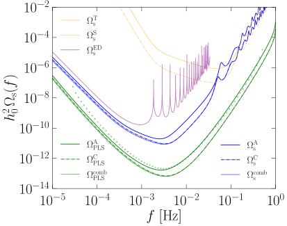
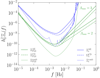
Figure 16: Sensitivities and PLS to GW energy density $\Omega_{\rm s}(f)$ (left panel) and helicity $\Xi_{\rm s}(f)$ (right panel) of LISA (‘A’), Taiji (‘C’), and the combined LISA–Taiji network (‘comb’); see Appendix B.4. The PLS are computed for a ${\rm SNR}=10$ and $T=4$ years of duration of the mission. The polarization PLS are computed limiting the maximum slope of the power law ${\Xi}_{\rm GW}(f)=C_{\beta}^{\rm pol}f^{\beta}$ to $\beta_{\rm max}=2$ and $3$; see figure 17 for larger values of $\beta_{\rm max}$. The sensitivities of the LISA $T$ and Taiji $S$ null channels are much larger at low frequencies than the other channels, so they are insensitive to GW signals (left panel). The cross-correlations between LISA and Taiji channels yield a monopole sensitivity to a polarized GW background; see $\Xi_{\rm s}^{\rm comb}(f)$, which is smaller than the dipole sensitivity induced in LISA, $\Xi_{\rm s}^{AE}(f)$, and Taiji, $\Xi_{\rm s}^{CD}(f)$ (right panel), while their sensitivity to the GW energy density, e.g., $\Omega_{\rm s}^{ED}(f)$, is much larger compared to those of the self-correlations of LISA, $\Omega_{\rm s}^{A}(f)$, and Taiji, $\Omega_{\rm s}^{C}(f)$ (left panel). The combination of the last two, $\Omega_{\rm s}^{\rm comb}(f)$, does not enhance significantly the detectability of a single detector. We show in green dots the PLS reported in ref. [110] (left panel); see their figure (2), with a SNR of 10 and $T=4\,{\rm yr}$. Note that ref. [110] uses the $X$ LISA channel instead of $A$.

In the case of parity odd signals, observed via the induced dipole response function due to our proper motion in the LISA $A$ and $E$ channels, the polarization SNR of a stochastic GW background with helical spectrum ${\Xi}_{\rm GW}(f)$ is computed by integrating $S_{AE}(f)$ in time and frequency; see equation (B.21),

$$\,{\rm SNR}_{\rm pol}=\sqrt{{\rm SNR}_{AE}^{2}+{\rm SNR}_{EA}^{2}}=\sqrt{2}\,{\rm SNR}_{AE}=$$

$$\,4\sqrt{T_{1\,{\rm yr}}}\left[\int_{0}^{T/(1\,{\rm yr})}\cos^{2}\alpha(x)\,{\rm d}{}x\int_{0}^{\infty}{\rm d}{}f\left(\frac{{\Xi}_{\rm GW}(f)-{\textstyle{1\over 4}}f{\rm d}{}{\Xi}_{\rm GW}(f)/{\rm d}{}\ln f}{\Xi_{\rm s}^{AE}(f)}\right)^{2}\right]^{1/2}.$$ (B.32)

The integral in time of $\cos^{2}\alpha(t)$ has been computed in ref. [79] assuming a circular orbit of LISA,

$$\int_{0}^{1}\cos^{2}\alpha(x)\,{\rm d}{}x=\frac{5+\cos 2(\theta_{v})}{16}\in(0.25,0.375),$$ (B.33)

where $\theta_{v}$ is the angle of the peculiar velocity. We take the minimum value of the integral, i.e., 0.25. Introducing this value into equation (B.32), the resulting SNR is

$${\rm SNR}_{\rm pol}=2\sqrt{T}\left[\int_{0}^{\infty}{\rm d}{}f\left(\frac{{\Xi}_{\rm GW}(f)-{\textstyle{1\over 4}}f{\rm d}{}{\Xi}_{\rm GW}(f)/{\rm d}{}\ln f}{\Xi_{\rm s}^{AE}(f)}\right)^{2}\right]^{1/2}.$$ (B.34)

To obtain the PLS of a polarized GW signal, as before, we consider a power law helical spectrum ${\Xi}_{\rm GW}(f)=C_{\beta}^{\rm pol}f^{\beta}$. We find that a special case is $\beta=4$, for which the polarization SNR is identically zero, and hence, such a signal is not detectable, independently of its amplitude. For values $\beta\neq 4$, the constant $C_{\beta}^{\rm pol}$ is

$$C_{\beta}^{\rm pol}=\frac{{\rm SNR}_{\rm pol}}{2\sqrt{T}|1-\beta/4|}\left[\int{\rm d}{}f\frac{f^{2\beta}}{[\Xi_{\rm s}^{AE}(f)]^{2}}\right]^{-1/2}.$$ (B.35)

Thus, we construct the PLS by taking the largest value of the function $C_{\beta}^{\rm pol}f^{\beta}$ in the range of $\beta$. Note that the same result applies to Taiji using $\Xi_{\rm s}^{CD}(f)$ in equations (B.32)–(B.35). The resulting polarization PLS curves of LISA and Taiji are shown in figure 17.

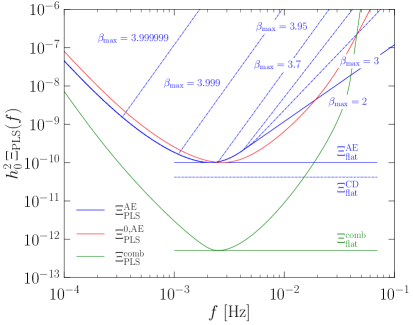
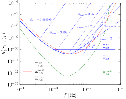
Figure 17: PLS to helical GW signals of LISA, $\Xi^{\rm AE}_{\rm PLS}(f)$ (left panel), and Taiji, $\Xi^{\rm CD}_{\rm PLS}(f)$ (right panel), computed for a ${\rm SNR}_{\rm pol}=10$ and $T=4$ years of duration of the mission, assuming power law slopes up to $\beta_{\rm max}=2$, $3$, $3.7$, $3.95$, $3.999\equiv 4-10^{-3}$, and $3.999999\equiv 4-10^{-6}$. The ${\rm SNR}_{\rm pol}$ is identically 0 when $\beta=4$, such that in the limit $\beta\rightarrow 4$, the helical signal cannot be detected; see equation (B.34). The PLS that would be obtained ignoring the ${\rm d}{}{\Xi}_{\rm GW}(f)/{\rm d}{}\ln f$ term, $\Xi_{\rm PLS}^{0}(f)$, and the PLS obtained by combining the cross-correlated channels of the LISA–Taiji network, $\Xi_{\rm PLS}^{\rm comb}(f)$; see Appendix B.4, are shown for comparison. The horizontal lines correspond to the flat spectra yielding a ${\rm SNR}_{\rm pol}=10$: $h_{0}^{2}\,\Xi^{AE}_{\rm flat}=10^{-10}$, $h_{0}^{2}\,\Xi^{CD}_{\rm flat}=4.16\times 10^{-11}$, and $h_{0}^{2}\,\Xi^{\rm comb}_{\rm flat}=5.1\times 10^{-13}$; see equations (4.10)–(4.12). The helical PLS computed in ref. [64]; see their figure (7), is shown in blue dots (right panel), compared to the PLS obtained considering $\beta\in(-20,2)\cup(5,20)$, which shows a change of slope from $\beta=2$ to $\beta=5$ around $10^{-2}\,{\rm Hz}$.

As the value of $\beta$ gets close to $4$, the denominator in equation (B.35) becomes larger, yielding large amplitudes of the PLS at a cutoff frequency that becomes smaller as we get closer to $4$. We compute the PLS curves for $\beta\in(-20,\beta_{\rm max})$ with $\beta_{\rm max}\in[2,4-10^{-6}]$ and observe a change of slope toward $\beta_{\rm max}$ at the cutoff frequency. For slopes $\beta\leq 3$, the cutoff occurs at a frequency larger than the sensitivity peak, such that the potential detectability is barely affected by the cutoff. However, if the helical GW signal has a slope between $3$ and $3.95$, the ${\rm SNR}_{\rm pol}$ is close to zero and the detectability at slightly larger frequencies than the sensitivity peak is more challenging; see figure 17. At even larger slopes, between 3.95 and 4, the cutoff frequency is below the peak sensitivity and the ${\rm SNR}_{\rm pol}$ goes asymptotically to zero. An analogous behavior is obtained when computing the PLS to GW signals with slopes larger than $4$, e.g., by taking a range $\beta\in(-20,3)\cup(\beta_{\rm min},20)$ with $\beta_{\rm min}>4$. For slopes $\beta_{\rm min}\geq 4.2$, the change of slope occurs at frequencies larger than $5\times 10^{-3}$ (same as for $\beta_{\rm max}=3$). Hence, for slopes $\beta\geq 4.2$, the potential detectability is again unaffected by the cutoff. The resulting PLS taking $\beta_{\rm min}=5$ is shown in the right panel of figure 17, compared to the PLS of ref. [64]; see their figure 7.

In the present work, we used the resulting helical PLS of LISA, $\Xi_{\rm PLS}^{AE}(f)$, and Taiji, $\Xi_{\rm PLS}^{CD}(f)$, obtained by taking power law spectra with slopes in the range $\beta\in(-20,3)\cup(4.2,20)$, which is valid for helical GW signals with slopes that are not between 3 and 4.2. The resulting PLS of LISA and Taiji are used in figures 12 and 13 to study the potential detectability of the polarized GW signals produced by primordial magnetic fields, computed from numerical simulations of MHD turbulence.

B.4 LISA–Taiji network

We now consider the possible combination of a network of space-based GW detectors, e.g., LISA and Taiji, following ref. [81]. In first place, the total SNR obtained by combining the self-correlations of the LISA and Taiji channels (i.e., the correlations between two channels of the same detector) is

$${\rm SNR}= \,\sqrt{{\rm SNR}_{AA}^{2}+{\rm SNR}_{EE}^{2}+{\rm SNR}_{CC}^{2}+{\rm SNR}_{DD}^{2}}=\sqrt{2({\rm SNR}^{2}_{AA}+{\rm SNR}_{CC}^{2})}$$

$$= \,2\sqrt{T}\left[\int{\rm d}{}f\,{\Omega}_{\rm GW}^{2}(f)\left(\frac{1}{[\Omega_{\rm s}^{A}(f)]^{2}}+\frac{1}{[\Omega_{\rm s}^{C}(f)]^{2}}\right)\right]^{1/2}$$

$$= \,2\sqrt{T}\left[\int{\rm d}{}f\left(\frac{{\Omega}_{\rm GW}(f)}{\Omega_{\rm s}^{\rm comb}(f)}\right)^{2}\right]^{1/2},$$ (B.36)

where we have defined the GW sensitivity of the combined LISA–Taiji network $\Omega_{\rm s}^{\rm comb}(f)$ (shown in figure 16),

$$\Omega_{\rm s}^{\text{\rm comb}}(f)=\left(\frac{1}{[\Omega_{\rm s}^{A}(f)]^{2}}+\frac{1}{[\Omega_{\rm s}^{C}(f)]^{2}}\right)^{-1/2}=\frac{\Omega_{\rm s}^{A}(f)\,\Omega_{\rm s}^{C}(f)}{\sqrt{[\Omega_{\rm s}^{A}(f)]^{2}+[\Omega_{\rm s}^{C}(f)]^{2}}}.$$ (B.37)

We again construct the PLS of the combined LISA–Taiji network $\Xi_{\rm PLS}^{\rm comb}(f)$; see figure 16, and see that the improvement is very small compared to the single detector (i.e., Taiji) PLS.

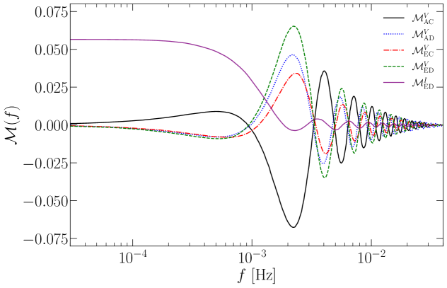
Figure 18: Helical response functions ${\cal M}^{V}_{OO^{\prime}}(f)$ of cross-correlated channels of LISA and Taiji, with $OO^{\prime}=AE$, $AD$, $EC$, and $ED$, and symmetric response function ${\cal M}^{I}_{ED}(f)$ [81], shown for comparison.

We now consider the cross-correlation response functions by combining different channels of LISA and Taiji. Similar to ref. [81], we define the $I$ and $V$ monopole response functions (for the $I$ and $V$ Stokes parameters) as

$${\cal M}_{OO^{\prime}}^{I}(f)={\textstyle{1\over 2}}\left({\cal M}_{OO^{\prime}}^{+}(f)+{\cal M}_{OO^{\prime}}^{-}(f)\right),\quad{\cal M}_{OO^{\prime}}^{V}(f)={\textstyle{1\over 2}}\left({\cal M}_{OO^{\prime}}^{+}(f)-{\cal M}_{OO^{\prime}}^{-}(f)\right),$$ (B.38)

with $O$ and $O^{\prime}=A$, $E$, $T$, $C$, $D$, or $S$, such that ${\cal M}_{OO^{\prime}}^{I}(f)$ and ${\cal M}_{OO^{\prime}}^{V}(f)$ contribute to the response functions to the GW energy density spectrum ${\Omega}_{\rm GW}(f)={\Omega}_{\rm GW}^{+}(f)+{\Omega}_{\rm GW}^{-}(f)$ and to the GW helicity spectrum ${\Xi}_{\rm GW}(f)={\Omega}_{\rm GW}^{+}(f)-{\Omega}_{\rm GW}^{-}(f)$, respectively. The contributions to the energy density sensitivity of the cross-correlated symmetric responses ${\cal M}_{OO^{\prime}}^{I}(f)$ are negligible, since their response functions are approximately zero at frequencies above $10^{-3}$, and smaller than the self-correlated responses ${\cal M}_{OO^{\prime}}^{V}(f)$, shown in figure 18 with ${\cal M}_{ED}^{I}(f)$ for comparison. The energy density sensitivity of the cross-correlated channels $OO^{\prime}=AE$, $AD$, $EC$, and $ED$; see equation (B.28), is

$$\Omega_{\rm s}^{OO^{\prime}}(f)=\frac{8\pi^{2}}{3H_{0}^{2}}f^{3}\frac{\sqrt{P_{n}^{O}(f)P_{n}^{O^{\prime}}(f)}}{{\cal M}_{OO^{\prime}}^{I}(f)},$$ (B.39)

which is shown in figure 16 with $OO^{\prime}=ED$ for comparison, where we can see that its sensitivity is much larger than the auto-correlation sensitivities $\Omega_{\rm s}^{A}(f)$ and $\Omega_{\rm s}^{C}(f)$ so we can omit their effect on the SNR and the PLS. Hence, the combination of LISA and Taiji does not significantly improve the detectability of a stochastic GW background signal ${\Omega}_{\rm GW}(f)$.

We now consider the sensitivity of the combined channels to a polarized GW background signal ${\Xi}_{\rm GW}(f)$. Figure 18 shows the $V$ response functions obtained by cross-correlating LISA and Taiji channels, such that the helical sensitivity can be defined as

$$\Xi_{\rm s}^{OO^{\prime}}(f)=\frac{8\pi^{2}}{3H_{0}^{2}}f^{3}\frac{\sqrt{P_{n}^{O}(f)P_{n}^{O^{\prime}}(f)}}{{\cal M}_{OO^{\prime}}^{V}(f)},$$ (B.40)

with $OO^{\prime}=AE$, $AD$, $EC$, and $ED$. We define the combined LISA–Taiji sensitivity as

$$\Xi_{\rm s}^{\rm comb}(f)= \,\left(\frac{1}{[\Xi_{\rm s}^{AC}(f)]^{2}}+\frac{1}{[\Xi_{\rm s}^{AD}(f)]^{2}}+\frac{1}{[\Xi_{\rm s}^{EC}(f)]^{2}}+\frac{1}{[\Xi_{\rm s}^{ED}(f)]^{2}}\right)^{-1/2}$$

$$= \,\frac{\Xi_{\rm s}^{AC}(f)\,\Xi_{\rm s}^{AD}(f)\,\Xi_{\rm s}^{EC}(f)\,\Xi_{\rm s}^{ED}(f)}{\sqrt{[\Xi_{\rm s}^{AC}(f)]^{2}+[\Xi_{\rm s}^{AD}(f)]^{2}+[\Xi_{\rm s}^{EC}(f)]^{2}+[\Xi_{\rm s}^{ED}(f)]^{2}}},$$ (B.41)

such that the corresponding polarization ${\rm SNR}_{\rm pol}$ is

$${\rm SNR}_{\rm pol}= \,\sqrt{2\left({\rm SNR}_{AC}^{2}+{\rm SNR}_{AD}^{2}+{\rm SNR}_{EC}^{2}+{\rm SNR}_{ED}^{2}\right)}$$

$$= \,2\sqrt{T} \left[\int{\rm d}{}f\,\left(\frac{{\Xi}_{\rm GW}(f)}{\Xi_{\rm s}^{\text{comb}}(f)}\right)^{2}\right]^{1/2}.$$ (B.42)

The resulting helical GW sensitivity and PLS, $\Xi_{\rm s}^{\rm comb}(f)$ and $\Xi_{\rm PLS}^{\rm comb}(f)$, respectively, of the combined LISA–Taiji network are shown in figure 16. We use the resulting PLS to study the potential detectability of polarized GW signals produced by primordial magnetic fields in section 4.3; see figures 12 and 13.

References

• [1] D. V. Deryagin, D. Y. Grigoriev, V. A. Rubakov and M. V. Sazhin, Possible anisotropic phases in the early universe and gravitational wave background, Mod. Phys. Lett. A 1, 593 (1986).
• [2] D. Grasso and H. R. Rubinstein, Magnetic fields in the early universe, Phys. Rept. 348, 163 (2001).
• [3] L. M. Widrow, Origin of galactic and extragalactic magnetic fields, Rev. Mod. Phys. 74, 775 (2002).
• [4] C. J. Hogan, Gravitational radiation from cosmological phase transitions, Mon. Not. Roy. Astron. Soc. 218, 629 (1986).
• [5] L. M. Krauss, Gravitational waves from global phase transitions, Phys. Lett. B 284, 229 (1992).
• [6] A. Kosowsky, M. S. Turner and R. Watkins, Gravitational waves from first order cosmological phase transitions, Phys. Rev. Lett. 69, 2026 (1992).
• [7] P. Amaro-Seoane et al.  [LISA], Laser Interferometer Space Antenna, arXiv:1702.00786 [astro-ph.IM] (2017).
• [8] J. Luo et al.  [TianQin], TianQin: A space-borne gravitational wave detector, Class. Quant. Grav. 33, 035010 (2016).
• [9] W. H. Ruan, Z. K. Guo, R. G. Cai and Y. Z. Zhang, Taiji program: Gravitational-wave sources, Int. J. Mod. Phys. A 35, 2050075 (2020).
• [10] M. Kamionkowski, A. Kosowsky and M. S. Turner, Gravitational radiation from first order phase transitions, Phys. Rev. D 49, 2837 (1994).
• [11] A. Kosowsky, A. Mack and T. Kahniashvili, Gravitational radiation from cosmological turbulence, Phys. Rev. D 66, 024030 (2002).
• [12] R. Apreda, M. Maggiore, A. Nicolis and A. Riotto, Gravitational waves from electroweak phase transitions, Nucl. Phys. B 631, 342 (2002).
• [13] A. D. Dolgov, D. Grasso and A. Nicolis, Relic backgrounds of gravitational waves from cosmic turbulence, Phys. Rev. D 66, 103505 (2002).
• [14] C. Grojean and G. Servant, Gravitational waves from phase transitions at the electroweak scale and beyond, Phys. Rev. D 75, 043507 (2007).
• [15] T. Kahniashvili, A. Kosowsky, G. Gogoberidze and Y. Maravin, Detectability of gravitational waves from phase transitions, Phys. Rev. D 78, 043003 (2008).
• [16] M. Hindmarsh, S. J. Huber, K. Rummukainen and D. J. Weir, Gravitational waves from the sound of a first order phase transition, Phys. Rev. Lett. 112, 041301 (2014).
• [17] D. J. Weir, Gravitational waves from a first order electroweak phase transition: A brief review, Phil. Trans. Roy. Soc. Lond. A 376, 20170126 (2018).
• [18] C. Caprini, M. Chala, G. C. Dorsch, M. Hindmarsh, S. J. Huber, T. Konstandin, J. Kozaczuk, G. Nardini, J. M. No and K. Rummukainen et al., Detecting gravitational waves from cosmological phase transitions with LISA: An update, JCAP 03, 024 (2020).
• [19] N. Seto, S. Kawamura and T. Nakamura, Possibility of direct measurement of the acceleration of the universe using 0.1-Hz band laser interferometer gravitational wave antenna in space, Phys. Rev. Lett. 87, 221103 (2001).
• [20] S. Phinney et al., The Big Bang Observer: Direct detection of gravitational waves from the birth of the Universe to the present, NASA Mission Concept Study (2004).
• [21] J. Crowder and N. J. Cornish, Beyond LISA: Exploring future gravitational wave missions, Phys. Rev. D 72, 083005 (2005).
• [22] E. Witten, Cosmic separation of phases, Phys. Rev. D 30, 272 (1984).
• [23] M. Signore and N. Sanchez, Comments on cosmological gravitational waves background and pulsar timings, Modern Physics Letters A, 4, 799 (1989).
• [24] S. E. Thorsett and R. J. Dewey, Pulsar timing limits on very low frequency stochastic gravitational radiation, Phys. Rev. D 53, 3468 (1996).
• [25] C. Caprini and D. G. Figueroa, Cosmological backgrounds of gravitational waves, Class. Quant. Grav. 35, 163001 (2018).
• [26] M. Kamionkowski, A. Kosowsky and A. Stebbins, A probe of primordial gravity waves and vorticity, Phys. Rev. Lett. 78, 2058 (1997).
• [27] U. Seljak and M. Zaldarriaga, Signature of gravity waves in polarization of the microwave background, Phys. Rev. Lett. 78, 2054 (1997).
• [28] A. A. Starobinsky, Cosmic background anisotropy induced by isotropic flat-spectrum gravitational-wave perturbations, Sov. Astron. Lett. 11, 133 (1985).
• [29] A. G. Polnarev, Polarization and anisotropy induced in the microwave background by cosmological gravitational waves, Sov. Astron. 29, 607 (1985).
• [30] L. A. Boyle and A. Buonanno, Relating gravitational wave constraints from primordial nucleosynthesis, pulsar timing, laser interferometers, and the CMB: Implications for the early Universe, Phys. Rev. D 78, 043531 (2008).
• [31] A. G. A. Brown et al.  [Gaia], Gaia data release 2: Summary of the contents and survey properties, Astron. Astrophys. 616, A1 (2018).
• [32] C. Boehm et al.  [Theia], Theia: Faint objects in motion or the new astrometry frontier, arXiv:1707.01348 [astro-ph.IM] (2017).
• [33] C. J. Moore, D. P. Mihaylov, A. Lasenby and G. Gilmore, Astrometric search method for individually resolvable gravitational wave sources with Gaia, Phys. Rev. Lett. 119, 261102 (2017).
• [34] J. Garcia-Bellido, H. Murayama and G. White, Exploring the Early Universe with Gaia and Theia, JCAP 12, 023 (2021).
• [35] A. Neronov and I. Vovk, Evidence for strong magnetic fields from Fermi observations of TeV blazars, Science 328, 73 (2010).
• [36] T. Vachaspati, Progress on cosmological magnetic fields, Rept. Prog. Phys. 84, 074901 (2021).
• [37] J. Ahonen and K. Enqvist, Electrical conductivity in the early universe, Phys. Lett. B 382, 40 (1996).
• [38] A. Brandenburg, K. Enqvist and P. Olesen, Large-scale magnetic fields from hydromagnetic turbulence in the very early universe, Phys. Rev. D 54, 1291 (1996).
• [39] A. Brandenburg, T. Kahniashvili, S. Mandal, A. Roper Pol, A. G. Tevzadze and T. Vachaspati, Evolution of hydromagnetic turbulence from the electroweak phase transition, Phys. Rev. D 96, 123528 (2017).
• [40] A. Brandenburg, T. Kahniashvili, S. Mandal, A. Roper Pol, A. G. Tevzadze and T. Vachaspati, Dynamo effect in decaying helical turbulence, Phys. Rev. Fluids 4, 024608 (2019).
• [41] D. Biskamp and W.-C. Müller, Decay laws for three-dimensional magnetohydrodynamic turbulence, Phys. Rev. Lett. 83, 2195 (1999).
• [42] M. Christensson, M. Hindmarsh and A. Brandenburg, Inverse cascade in decaying 3D magnetohydrodynamic turbulence, Phys. Rev. E 64, 056405 (2001).
• [43] T. Vachaspati, Magnetic fields from cosmological phase transitions, Phys. Lett. B 265, 258 (1991).
• [44] T. Vachaspati, Estimate of the primordial magnetic field helicity, Phys. Rev. Lett. 87, 251302 (2001).
• [45] J. M. Cornwall, Speculations on primordial magnetic helicity, Phys. Rev. D 56, 6146 (1997).
• [46] M. Joyce and M. E. Shaposhnikov, Primordial magnetic fields, right-handed electrons, and the Abelian anomaly, Phys. Rev. Lett. 79, 1193 (1997).
• [47] J. García-Bellido, D. Y. Grigoriev, A. Kusenko and M. E. Shaposhnikov, Nonequilibrium electroweak baryogenesis from preheating after inflation, Phys. Rev. D 60, 123504 (1999).
• [48] J. M. Cornwall and A. Kusenko, Baryon number nonconservation and phase transitions at preheating, Phys. Rev. D 61, 103510 (2000).
• [49] J. García-Bellido, M. García Pérez and A. González-Arroyo, Symmetry breaking and false vacuum decay after hybrid inflation, Phys. Rev. D 67, 103501 (2003).
• [50] J. García-Bellido, M. García-Pérez and A. González-Arroyo, Chern-Simons production during preheating in hybrid inflation models, Phys. Rev. D 69, 023504 (2004).
• [51] A. Díaz-Gil, J. García-Bellido, M. García Pérez and A. González-Arroyo, Magnetic field production during preheating at the electroweak scale, Phys. Rev. Lett. 100, 241301 (2008).
• [52] M. M. Forbes and A. R. Zhitnitsky, Primordial galactic magnetic fields from domain walls at the QCD phase transition, Phys. Rev. Lett. 85, 5268 (2000).
• [53] L. Campanelli and M. Giannotti, Magnetic helicity generation from the cosmic axion field, Phys. Rev. D 72, 123001 (2005).
• [54] M. S. Turner and L. M. Widrow, Inflation produced, large scale magnetic fields, Phys. Rev. D 37, 2743 (1988).
• [55] B. Ratra, Cosmological ‘seed’ magnetic field from inflation, Astrophys. J. Lett. 391, L1 (1992).
• [56] W. D. Garretson, G. B. Field and S. M. Carroll, Primordial magnetic fields from pseudoGoldstone bosons, Phys. Rev. D 46, 5346 (1992).
• [57] A. Dolgov, Breaking of conformal invariance and electromagnetic field generation in the universe, Phys. Rev. D 48, 2499 (1993).
• [58] M. Gasperini, M. Giovannini and G. Veneziano, Primordial magnetic fields from string cosmology, Phys. Rev. Lett. 75, 3796 (1995).
• [59] R. Durrer and A. Neronov, Cosmological magnetic fields: Their generation, evolution and observation, Astron. Astrophys. Rev. 21, 62 (2013).
• [60] K. Subramanian, The origin, evolution and signatures of primordial magnetic fields, Rept. Prog. Phys. 79, 076901 (2016).
• [61] M. Giovannini, Magnetic knots as the origin of spikes in the gravitational wave backgrounds, Phys. Rev. D 58, 124027 (1998).
• [62] T. Kahniashvili, G. Gogoberidze, and B. Ratra, Polarized cosmological gravitational waves from primordial helical turbulence, Phys. Rev. Lett. 95, 151301 (2005).
• [63] L. Kisslinger and T. Kahniashvili, Polarized gravitational waves from cosmological phase transitions, Phys. Rev. D 92, 043006 (2015).
• [64] J. Ellis, M. Fairbairn, M. Lewicki, V. Vaskonen and A. Wickens, Detecting circular polarisation in the stochastic gravitational-wave background from a first-order cosmological phase transition, JCAP 10, 032 (2020).
• [65] T. Kahniashvili, A. Brandenburg, G. Gogoberidze, S. Mandal and A. Roper Pol, Circular polarization of gravitational waves from early-Universe helical turbulence, Phys. Rev. Res. 3, 013193 (2021).
• [66] N. Seto, Prospects for direct detection of circular polarization of gravitational-wave background, Phys. Rev. Lett. 97, 151101 (2006).
• [67] N. Seto, Quest for circular polarization of gravitational wave background and orbits of laser interferometers in space, Phys. Rev. D 75, 061302 (2007).
• [68] A. D. Sakharov, Violation of CP Invariance, C asymmetry, and baryon asymmetry of the universe, Pisma Zh. Eksp. Teor. Fiz. 5, 32 (1967).
• [69] V. A. Kuzmin, V. A. Rubakov and M. E. Shaposhnikov, On the anomalous electroweak baryon number nonconservation in the early Universe, Phys. Lett. B 155, 36 (1985).
• [70] M. E. Shaposhnikov, Possible appearance of the baryon asymmetry of the Universe in an electroweak theory, JETP Lett. 44, 465 (1986).
• [71] A. G. Cohen, D. B. Kaplan and A. E. Nelson, Weak scale baryogenesis, Phys. Lett. B 245, 561 (1990).
• [72] A. G. Cohen, D. B. Kaplan and A. E. Nelson, Baryogenesis at the weak phase transition, Nucl. Phys. B 349, 727 (1991).
• [73] D. E. Morrissey and M. J. Ramsey-Musolf, Electroweak baryogenesis, New J. Phys. 14, 125003 (2012).
• [74] T. Fujita and K. Kamada, Large-scale magnetic fields can explain the baryon asymmetry of the Universe, Phys. Rev. D 93, 083520 (2016).
• [75] K. Kamada and A. J. Long, Baryogenesis from decaying magnetic helicity, Phys. Rev. D 94, 063501 (2016).
• [76] K. Kamada and A. J. Long, Evolution of the baryon asymmetry through the electroweak crossover in the presence of a helical magnetic field, Phys. Rev. D 94, 123509 (2016).
• [77] R. H. Kraichnan, Inertial-range spectrum of hydromagnetic turbulence, Phys. Fluids 8 (1965).
• [78] S. S. Moiseev and O. G. Chkhetiani, Helical scaling in turbulence, Sov. Phys. JETP 83, 192 (1996).
• [79] V. Domcke, J. García-Bellido, M. Peloso, M. Pieroni, A. Ricciardone, L. Sorbo and G. Tasinato, Measuring the net circular polarization of the stochastic gravitational wave background with interferometers, JCAP 05, 028 (2020).
• [80] N. Seto, Measuring parity asymmetry of gravitational wave backgrounds with a heliocentric detector network in the mHz band, Phys. Rev. Lett. 125, 251101 (2020).
• [81] G. Orlando, M. Pieroni and A. Ricciardone, Measuring parity violation in the stochastic gravitational wave background with the LISA-Taiji network, JCAP 03, 069 (2021).
• [82] A. Roper Pol, S. Mandal, A. Brandenburg, T.  Kahniashvili and A. Kosowsky, Numerical simulations of gravitational waves from early-universe turbulence, Phys. Rev. D 102, 083512 (2020).
• [83] A. Roper Pol, A. Brandenburg, T. Kahniashvili, A. Kosowsky and S. Mandal, The timestep constraint in solving the gravitational wave equations sourced by hydromagnetic turbulence, Geophys. Astrophys. Fluid Dynam. 114, 130 (2020).
• [84] A. Brandenburg, A. Johansen, P. A. Bourdin, W.  Dobler, W. Lyra, M. Rheinhardt, S. Bingert, N. E.  L. Haugen, A. Mee, F. Gent, N. Babkovskaia, C.-C.  Yang, T. Heinemann, B. Dintrans, D. Mitra, S. Candelaresi, J. Warnecke, P. J. Käpylä, A. Schreiber, P. Chatterjee, M. J. Käpylä, X.-Y. Li, J. Krüger, J. R. Aarnes, G. R. Sarson, J. S. Oishi, J. Schober, R. Plasson, C. Sandin, E. Karchniwy, L. F. S. Rodrigues, A. Hubbard, G. Guerrero, A. Snodin, I. R. Losada, J. Pekkilä, and C. Qian [Pencil Code Collaboration], The Pencil Code, a modular MPI code for partial differential equations and particles: multipurpose and multiuser-maintained, Journal of Open Source Software 6, 2807 (2021).
• [85] D. A. Varshalovich, A. N. Moskalev and V. K. Khersonsky, Quantum theory of angular momentum: Irreducible tensors, spherical harmonics, vector coupling coefficients, 3nj symbols, World Scientific, Singapore (1988).
• [86] W. Hu and M. J. White, CMB anisotropies: Total angular momentum method, Phys. Rev. D 56, 596 (1997).
• [87] L. P. Grishchuk, Amplification of gravitational waves in an isotropic universe, Sov. Phys. JETP 40, 409 (1974).
• [88] A. S. Monin and A. M. Yaglom. Statistical fluid mechanics of turbulence, vol. 2, MIT press, Cambridge U.K. (1975).
• [89] A. N. Kolmogorov, The local structure of turbulence in incompressible viscous fluid for very large Reynolds numbers, Proc. USSR Acad. Sci. 30, 301 (1941).
• [90] P. S. Iroshnikov, Turbulence of a conducting fluid in a strong magnetic field, Astron. Zh. 40, 742 (1963).
• [91] W. C. Müller and D. Biskamp, Scaling properties of three-dimensional magnetohydrodynamic turbulence, Phys. Rev. Lett. 84, 475 (2000).
• [92] H. K. Moffatt, Magnetic field generation in electrically conducting fluids, Cambridge Univ. Press, Cambridge, U.K. (1978).
• [93] C. W. Misner, K. S. Thorne and J. A. Wheeler, Gravitation, W. H. Freeman, San Francisco, USA (2017).
• [94] M. Maggiore, Gravitational wave experiments and early universe cosmology, Phys. Rept. 331, 283 (2000).
• [95] C. Caprini, R. Durrer and T. Kahniashvili, The cosmic microwave background and helical magnetic fields: The tensor mode, Phys. Rev. D 69, 063006 (2004).
• [96] A. Brandenburg and S. Boldyrev, The turbulent stress spectrum in the inertial and subinertial ranges, Astrophys. J. 892, 80 (2020).
• [97] E. W. Kolb and M. S. Turner, The early Universe, Front. Phys. 69, 1 (1990).
• [98] A. Brandenburg, G. Gogoberidze, T. Kahniashvili, S. Mandal, A. Roper Pol and N. Shenoy, The scalar, vector, and tensor modes in gravitational wave turbulence simulations, Class. Quantum Grav. 38, 145002 (2021).
• [99] A. Brandenburg, E. Clarke, Y. He and T. Kahniashvili, Can we observe the QCD phase transition-generated gravitational waves through pulsar timing arrays? Phys. Rev. D 104, 043513 (2021).
• [100] P. Niksa, M. Schlederer and G. Sigl, Gravitational waves produced by compressible MHD turbulence from cosmological phase transitions, Class. Quant. Grav. 35, 144001 (2018).
• [101] C. Caprini, R. Durrer and G. Servant, The stochastic gravitational wave background from turbulence and magnetic fields generated by a first-order phase transition, JCAP 12, 024 (2009).
• [102] C. Caprini, R. Durrer and X. Siemens, Detection of gravitational waves from the QCD phase transition with pulsar timing arrays, Phys. Rev. D 82, 063511 (2010).
• [103] P. Binetruy, A. Bohe, C. Caprini and J. F. Dufaux, Cosmological backgrounds of gravitational waves and eLISA/NGO: Phase transitions, cosmic strings and other sources, JCAP 06, 027 (2012).
• [104] G. Gogoberidze, T. Kahniashvili and A. Kosowsky, The spectrum of gravitational radiation from primordial turbulence, Phys. Rev. D 76, 083002 (2007).
• [105] N. Seto and A. Taruya, Measuring a parity violation signature in the early Universe via ground-based laser interferometers, Phys. Rev. Lett. 99, 121101 (2007).
• [106] K. Martinovic, C. Badger, M. Sakellariadou and V. Mandic, Searching for parity violation with the LIGO-Virgo-KAGRA network, Phys. Rev. D 104, L081101 (2021).
• [107] N. Seto and A. Taruya, Polarization analysis of gravitational-wave backgrounds from the correlation signals of ground-based interferometers: Measuring a circular-polarization mode, Phys. Rev. D 77, 103001 (2008).
• [108] S. G. Crowder, R. Namba, V. Mandic, S. Mukohyama and M. Peloso, Measurement of parity violation in the early Universe using gravitational-wave detectors, Phys. Lett. B 726, 66 (2013).
• [109] C. Caprini, M. Hindmarsh, S. Huber, T. Konstandin, J. Kozaczuk, G. Nardini, J. M. No, A. Petiteau, P. Schwaller and G. Servant et al., Science with the space-based interferometer eLISA. II: Gravitational waves from cosmological phase transitions, JCAP 04, 001 (2016).
• [110] C. Caprini, D. G. Figueroa, R. Flauger, G. Nardini, M. Peloso, M. Pieroni, A. Ricciardone and G. Tasinato, Reconstructing the spectral shape of a stochastic gravitational wave background with LISA, JCAP 11, 017 (2019).
• [111] J. D. Romano and N. J. Cornish, Detection methods for stochastic gravitational-wave backgrounds: A unified treatment, Living Rev. Rel. 20, 2 (2017).
• [112] J. R. Espinosa, T. Konstandin, J. M. No and G. Servant, Energy budget of cosmological first-order phase transitions, JCAP 06, 028 (2010).
• [113] K. Schmitz, New sensitivity curves for gravitational-wave signals from cosmological phase transitions, JHEP 01, 097 (2021).
• [114] V. F. Shvartsman, Density of relict particles with zero rest mass in the universe, Pisma Zh. Eksp. Teor. Fiz. 9, 315 (1969).
• [115] T. Kahniashvili, A. G. Tevzadze and B. Ratra, Phase transition generated cosmological magnetic field at large scales, Astrophys. J. 726, 78 (2011).
• [116] A. Brandenburg, Y. He, T. Kahniashvili, M. Rheinhardt and J. Schober, Relic gravitational waves from the chiral magnetic effect, Astrophys. J. 911, 110 (2021).
• [117] U. Frisch, A. Pouquet, J. Léorat and A. Mazure, Possibility of an inverse cascade of magnetic helicity in magnetohydrodynamic turbulence, Journal of Fluid Mechanics 68, 769 (1975).
• [118] A. Brandenburg and T. Kahniashvili, Classes of hydrodynamic and magnetohydrodynamic turbulent decay, Phys. Rev. Lett. 118, 055102 (2017).
• [119] A. Brandenburg and K. Subramanian, Minimal tau approximation and simulations of the alpha effect, Astron. Astrophys. 439, 835 (2005).
• [120] A. G. Tevzadze, L. Kisslinger, A. Brandenburg and T. Kahniashvili, Magnetic fields from QCD phase transitions, Astrophys. J. 759, 54 (2012).
• [121] D. Grasso and H. R. Rubinstein, Revisiting nucleosynthesis constraints on primordial magnetic fields, Phys. Lett. B 379, 73 (1996).
• [122] A. Roper Pol, S. Mandal, A. Brandenburg, and T. Kahniashvili, Datasets for “Polarization of gravitational waves from helical MHD turbulent sources” (v2021.09.24), DOI:10.5281/zenodo.5525504 (2021).
• [123] A. Roper Pol, GitHub project “GW_turbulence,” DOI:10.5281/zenodo.6045844.
• [124] W. H. Ruan, C. Liu, Z. K. Guo, Y. L. Wu and R. G. Cai, The LISA-Taiji network, Nature Astron. 4, 108 (2020).
• [125] M. R. Adams and N. J. Cornish, Discriminating between a stochastic gravitational wave background and instrument noise, Phys. Rev. D 82, 022002 (2010).
• [126] N. Bartolo, V. Domcke, D. G. Figueroa, J. García-Bellido, M. Peloso, M. Pieroni, A. Ricciardone, M. Sakellariadou, L. Sorbo and G. Tasinato, Probing non-Gaussian stochastic gravitational wave backgrounds with LISA, JCAP 11, 034 (2018).
• [127] T. Robson, N. J. Cornish and C. Liu, The construction and use of LISA sensitivity curves, Class. Quant. Grav. 36, 105011 (2019).
• [128] R. Flauger, N. Karnesis, G. Nardini, M. Pieroni, A. Ricciardone and J. Torrado, Improved reconstruction of a stochastic gravitational wave background with LISA, JCAP 01, 059 (2021).
• [129] LISA Science Requirements Document, available at https://www.cosmos.esa.int/web/lisa/lisa-documents