Low frequency tail of gravitational wave spectra from hydromagnetic turbulence

Abstract

Hydrodynamic and magnetohydrodynamic (MHD) turbulence in the early Universe can drive gravitational waves (GWs) and imprint their spectrum onto that of GWs, which might still be observable today. We study the production of the GW background from freely decaying MHD turbulence from helical and nonhelical initial magnetic fields. To understand the produced GW spectra, we develop a simple model on the basis of the evolution of the magnetic stress tensor. We find that the GW spectra obtained in this model reproduce those obtained in numerical simulations if we consider the detailed time evolution of the low frequency tail of the stress spectrum from numerical simulations. We also show that the shapes of the produced GW frequency spectra are different for helical and nonhelical cases for the same initial magnetic energy spectra. Such differences can help distinguish helical and nonhelical initial magnetic fields from a polarized background of GWs – especially when the expected circular polarization cannot be detected directly.

I Introduction

Magnetohydrodynamic (MHD) turbulence in the early Universe can be a powerful source of gravitational waves (GWs) that could be observable as a stochastic background today (Kamionkowski et al., 1994; Hogan, 2000; Kosowsky et al., 2002; Dolgov et al., 2002; Caprini and Figueroa, 2018). The frequency spectrum of these waves is related to the spectrum of the underlying turbulence. Such turbulence could be induced during the various epochs in the early Universe (Witten, 1984, 1984; Hogan, 1986; Mazumdar and White, 2019; Hindmarsh et al., 2021) or the possible presence of primordial magnetic fields (Turner and Widrow, 1988; Vachaspati, 1991; Ratra, 1992; Durrer and Neronov, 2013; Subramanian, 2016, 2019; Vachaspati, 2021; Brandenburg et al., 2021). These GWs produced by turbulence at an epoch of the electroweak phase transition lie in the sensitivity range of the proposed Laser Interferometer Space Antenna and pulsar timing arrays for the turbulence induced around an epoch of the quantum chromodynamics (QCD) phase transition. Recently, various pulsar timing arrays (Arzoumanian et al., 2020; Goncharov et al., 2021; Chen et al., 2021; Antoniadis et al., 2022) have reported evidence for the presence of a common spectrum process across analyzed pulsars in the search of the presence of an isotropic stochastic GW background. This evidence has been used to constrain the strength and correlation length of magnetic fields generated at the QCD epoch (Neronov et al., 2021; Sharma, 2022; Roper Pol et al., 2022a). However, the presence of a quadrupolar spatial correlation (Hellings and Downs, 1983), a characteristics of a GW background, is yet to be claimed.

Numerical simulations have confirmed that there is indeed a direct connection between the slopes of the turbulence and GW spectra (Roper Pol et al., 2020a), except that at low frequencies, below the peak of the spectrum, the GW spectrum was found to be shallower in the simulations than what was previously expected from analytical calculations. We call this part the low frequency tail of the GW spectrum. However, there is the worry that this shallow tail could be caused by unknown numerical artifacts such as the finite size of the computational domain and the way the turbulence is initiated in the simulations.

To understand the origin of the low frequency tail, the authors of Ref. Roper Pol et al. (2022a) have recently compared numerical MHD simulations with an analytic model, where the stress is assumed constant for a certain interval of time. Their model predicts a flat spectrum whose extent depends on the duration over which the stress is held constant. In this way, it was possible to determine an effective duration for a given numerical simulation. This duration was found to be different for different simulations. Their model is therefore descriptive rather than predictive. Furthermore, in the numerical solutions the stress was not actually constant for any duration of time.

In another recent approach, the authors of Ref. Auclair et al. (2022) have focused on the importance of unequal time correlation functions of the Fourier components of the velocity field for purely hydrodynamic turbulence. While the authors acknowledge the potential importance of the initial growth phase of the turbulence, they also have no inverse cascade in their simulations. This is different from MHD turbulence, which can display inverse cascading even in the absence of net magnetic helicity Brandenburg et al. (2015); Zrake (2014). This will be crucial to the approach discussed in the present paper.

To address the problem of a limited computational domain, it is important to use large enough computational domains so that its minimum wave number is as small as possible. In this paper, we discuss two MHD simulations where the wave number corresponding to the peak of the GW spectrum and the wave numbers below that corresponding to the horizon size at the initial time are well resolved. Since the stress appears explicitly in the linearized GW equation, we also analyze for these simulations the evolution of the stress spectrum along with the magnetic and GW spectra. Such a detailed comparison between the simulated stress and resulting GWs is an important new aspect of the present work. Second, we develop a simple model, motivated by the stress evolution seen in the present simulations, to explain the GW spectrum obtained. In this model, our main focus is to understand the nature of the GW spectrum below the wave number corresponding to the peak of the spectrum. Our simulations are similar to those of Ref. Roper Pol et al. (2022a), but our interpretation and corresponding modeling of the stress is not. There is no time interval during which the stress is constant. Our results are therefore not characterized by the duration of such a time interval. In addition, we determine and analyze spectral differences between runs with and without magnetic helicity, which were not noticed previously. We also emphasize that the Hubble horizon wave number poses an ultimate cutoff for the flat spectrum toward low wave numbers.

This paper is organized as follows. In Section II, we discuss the evolution of the magnetic field, stress, and GW spectrum in our new runs. In this section, we also discuss how the stress spectrum evolves when inverse transfer and inverse cascade of the turbulence correspond to the evolution for nonhelical and helical magnetic fields in the early Universe. In Section III, we discuss the model to explain the low frequency tail of the GW spectrum. Further, in Section IV, we compare the GW spectrum obtained from our numerical simulations and our model. We conclude in Section V.

II Nonhelical and helical cascades

Various phenomena such as primordial magnetic fields and phase transitions can lead to the generation of turbulence in the early Universe. The stress associated with magnetic fields and turbulence lead to the production of GWs. This has been studied in the literature both analytically (Dolgov et al., 2002; Kosowsky et al., 2002; Gogoberidze et al., 2007; Kahniashvili et al., 2008; Caprini et al., 2009; Niksa et al., 2018; Sharma et al., 2020) and numerically (Roper Pol et al., 2020a, 2022b; Kahniashvili et al., 2021; Dahl et al., 2021; Roper Pol et al., 2022a; Auclair et al., 2022). In the present paper, we perform new simulations of decaying MHD turbulence, where we resolve the scales which are smaller than the Hubble horizon size at the initial time. Before explaining the simulations in detail, let us begin by summarizing the basic equations.

II.1 GWs from MHD turbulence

We follow here the formalism of Ref. Roper Pol et al. (2020b, a), where conformal time is normalized to unity at the initial time. One could associate this with the electroweak phase transition, for example. The velocity $\mathbf{u}$ is normalized to the speed of light. The magnetic field $\mathbf{B}={\mathbf{\nabla}}\times\mathbf{A}$ is written in terms of the magnetic vector potential $\mathbf{A}$, and the current density is written as $\mathbf{J}={\mathbf{\nabla}}\times\mathbf{B}$. Following Ref. Brandenburg et al. (1996), the energy density $\rho$ includes the restmass density, so its evolution equation obeys a continuity equation that also includes magnetic energy terms. As in Roper Pol et al. (2020b), $\rho$ is normalized to the critical energy density for a flat Universe. We solve for the Fourier transformed plus and cross polarizations of the gravitational strain, $\tilde{h}_{+}$ and $\tilde{h}_{\times}$, which are driven by the corresponding projections of the stress, which, in turn, is composed of kinetic and magnetic contributions,

$${\sf T}_{ij}=\frac{4}{3}\gamma_{\rm Lor}^{2}\rho u_{i}u_{j}-B_{i}B_{j}+...,$$ (1)

where $\gamma_{\rm Lor}=(1-\mathbf{u}^{2})^{-1/2}$ is the Lorentz factor, and the ellipsis denotes terms proportional to $\delta_{ij}$, which do not contribute to the projected source $\tilde{T}_{+/\times}$.

Assuming the Universe to be conformally flat, its expansion can be scaled out by working with conformal time $t$ and comoving variables (Brandenburg et al., 1996). We use the fact that in the radiation-dominated era, the scale factor grows linearly with conformal time. The only explicit occurrence of conformal time is then in the GW equation, where a $6/t$ factor occurs in the source term (Roper Pol et al., 2020b). The full set of equations is therefore

$$\frac{\partial\mathbf{B}}{\partial t}={\mathbf{\nabla}}\times(\mathbf{u}\times\mathbf{B}-\eta{\mathbf{\nabla}}\times\mathbf{B}),$$ (2)

$${{\rm D}{}\mathbf{u}\over{\rm D}{}t}={1\over\rho}{\mathbf{\nabla}}\cdot\left(2\rho\nu\mbox{\boldmath${\sf S}$}{}\right)-{1\over 4}{\mathbf{\nabla}}\ln\rho+{\mathbf{u}\over 3}\left({\mathbf{\nabla}}\cdot\mathbf{u}+\mathbf{u}\cdot{\mathbf{\nabla}}\ln\rho\right)$$

$$\qquad\quad-{\mathbf{u}\over\rho}\left[\mathbf{u}\cdot(\mathbf{J}\times\mathbf{B})+\eta\mathbf{J}^{2}\right]+{3\over 4\rho}\mathbf{J}\times\mathbf{B},$$ (3)

$${\partial\ln\rho\over\partial t}=-\frac{4}{3}\left({\mathbf{\nabla}}\cdot\mathbf{u}+\mathbf{u}\cdot{\mathbf{\nabla}}\ln\rho\right)+{1\over\rho}\left[\mathbf{u}\cdot(\mathbf{J}\times\mathbf{B})+\eta\mathbf{J}^{2}\right]\!,$$

$$\frac{\partial^{2}}{\partial t^{2}}\tilde{h}_{+/\times}(\mathbf{k},t)+k^{2}\tilde{h}_{+/\times}(\mathbf{k},t)={6\over t}\tilde{T}_{+/\times}(\mathbf{k},t),$$ (4)

where ${\rm D}{}/{\rm D}{}t\equiv\partial/\partial t+\mathbf{u}\cdot{\mathbf{\nabla}}$ is the advective derivative, $\eta$ is the magnetic diffusivity, $\nu$ is the kinematic viscosity, ${\sf S}_{ij}={\textstyle{1\over 2}}(u_{i,j}+u_{j,i})-{\textstyle{1\over 3}}\delta_{ij}{\mathbf{\nabla}}\cdot\mathbf{u}$ are the components of the rate-of-strain tensor ${\sf S}$ with commas denoting partial derivatives. Fourier transformation in space is denoted by a tilde. In all cases studied in this paper, the initial conditions are such that $\mathbf{B}$ consists of a weak Gaussian-distributed seed magnetic field, $\mathbf{u}=0$, $\rho=1$.

We work with spectra that are defined as integrals over concentric shells in wave number space $\mathbf{k}$ with $k=|\mathbf{k}|$. They are normalized such that their integrals over $k$ give the mean square of the corresponding quantity, i.e., $\int\mbox{\rm Sp}(\mathbf{B})\,{\rm d}{}k=\langle\mathbf{B}^{2}\rangle$, where $\mbox{\rm Sp}(\mathbf{B})=\mbox{\rm Sp}(B_{x})+\mbox{\rm Sp}(B_{y})+\mbox{\rm Sp}(B_{z})$. Similarly, $\mbox{\rm Sp}(\mbox{\boldmath${\sf h}$}{})=\mbox{\rm Sp}(h_{+})+\mbox{\rm Sp}(h_{\times})$ is defined as the sum over the two polarization modes. Of particular interest will also be the stress spectrum $\mbox{\rm Sp}(\mbox{\boldmath${\sf T}$}{})$, which is defined analogously through $\mbox{\rm Sp}(\mbox{\boldmath${\sf T}$}{})=\mbox{\rm Sp}(T_{+})+\mbox{\rm Sp}(T_{\times})$. To study the evolution of the stress at selected Fourier modes, we compute $|\tilde{T}(k,t)|\equiv\sqrt{\mbox{\rm Sp}(\mbox{\boldmath${\sf T}$}{})/4\pi k^{2}}$, which scales the same way as $|\tilde{T}_{+}(k,t)|$ and $|\tilde{T}_{\times}(k,t)|$.

II.2 Evolution of the stress and strain spectra

To put our results into perspective and compare with earlier work, we study cases of suddenly initiated turbulence. We perform simulations similar to those of Ref. Roper Pol et al. (2020a) by using as initial condition for the magnetic field a random Gaussian-distributed magnetic field with a $k^{4}$ spectrum for $k<k_{\rm p}$ and a $k^{-5/3}$ spectrum for $k>k_{\rm p}$. For details of such a magnetic field, see Ref. Brandenburg et al. (2017). As initial condition for the GW field, we assume that $h$ and $\dot{h}$ vanish. The strength of the GW field is then strongly determined by the sudden initialization of a fully developed turbulence spectrum. The details of the simulations are given in Table LABEL:table1. In this table, the first column represents the name of the runs (HEL and NHEL), ${\cal E}_{\rm EM}^{i}$ is the initial value of the magnetic energy density compared to the background energy density, $k_{\rm p}$ is the wave number at which the magnetic energy spectrum peaks and it is normalized by the wave number corresponding to the Hubble horizon size at the initial time, ${\cal E}_{\rm GW}^{\rm sat}$ is the value of the GW energy density after saturation compared to the background energy density, and ${\Omega}_{\rm GW}^{\rm sat}$ is the density parameter of GWs, representing the ratio of the GW energy density compared to the critical energy density at present. ${\Omega}_{\rm GW}^{\rm sat}$ has been calculated considering the production of GWs around the electroweak phase transition.

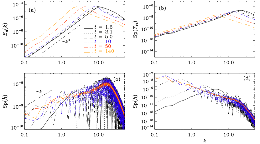
Figure 1: Spectra of the magnetic field, the TT-projected stress, the strain derivative, and the strain for suddenly initiated turbulence with magnetic helicity.

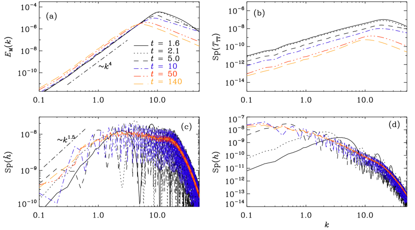
Figure 2: Same as Fig. 1, but for the nonhelical case.

We consider two runs where the initial magnetic field is either fully helical (HEL) or nonhelical (NHEL). In Figs. 1 and 2, we show for HEL and NHEL, respectively, the time evolution of the spectra of the magnetic field, the TT-projected stress, the strain derivative, and the strain. Inverse cascading is seen in the magnetic energy spectra, which leads to the expected increase of the spectral stress at small $k$; see Figs. 1(a) and (b) for the HEL run. By contrast, in NHEL, the stress spectrum always decreases at small $k$. We also see in Fig. 1(c) that the GW energy spectrum has a maximum at $k\approx 20$, which is not present in NHEL; cf. Fig. 2(c). Their spectra fall off toward smaller $k$ proportional to $k$ and $k^{1.5}$ for HEL and NHEL, respectively.

Table 1: Summary of simulation parameters

Run	${\cal E}_{\rm M}^{i}$	$k_{\rm p}$	${\cal E}_{\rm GW}^{\rm sat}$	${\Omega}_{\rm GW}^{\rm sat}$
HEL	$5.4\times 10^{-3}$	$10$	$3.7\times 10^{-7}$	$5.9\times 10^{-12}$
NHEL	$5.5\times 10^{-3}$	$10$	$3.5\times 10^{-7}$	$5.6\times 10^{-12}$

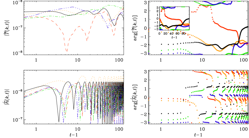
Figure 3: Modulus and phase of $\tilde{T}(k,t)$ and $\dot{\tilde{h}}(k,t)$ for the helical case for $\mathbf{k}=(k,0,0)$ with $k=0.3$ (orange), 0.4 (red), 0.5 (green), 0.6 (blue), and 0.7 (black). The inset shows the phase with a linear abscissa.

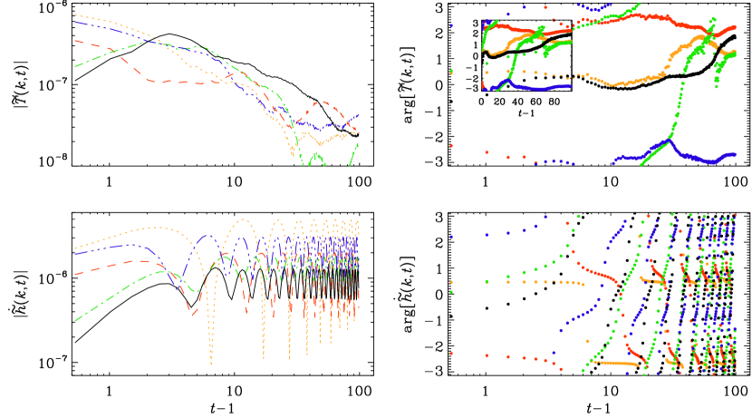
Figure 4: Same as Fig. 3, but for the nonhelical case.

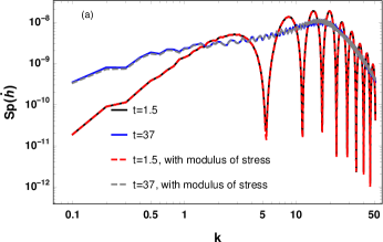
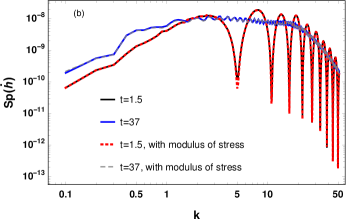
Figure 5: $\mbox{\rm Sp}(\dot{\mbox{\boldmath${\sf h}$}{}})(k,t)$ vs $k$: (a) The solid black and blue curves represent $\mbox{\rm Sp}(\dot{\mbox{\boldmath${\sf h}$}{}})(k,t)$ at times $t=1.5$ and $t=37$ for run hel. The dashed red and gray curves show $\mbox{\rm Sp}(\dot{\mbox{\boldmath${\sf h}$}{}})(k,t)$ for the case when the stress spectrum has been replaced by its modulus in the GW evolution equation. The black curve coincides with the dashed red curve and solid blue curve coincides with dashed gray curve. (b) Same as (a), but for run nonhel.

In Figs. 3 and 4, we show the time evolution of the modulus and phase of stress and strain derivative for HEL and NHEL for wave vectors $\mathbf{k}=(k,0,0)$ and five different values of $k$, which are all below $k_{\rm p}$. The purpose of this is to see how representative these individual wave vectors are compared to the collective effect of all others of similar length, and whether there is any important effect resulting from the phases of the stress.

Broadly speaking, the time evolution of the modulus of the stress $|\tilde{T}|$ for any of the five wave vectors does not seems to reflect the expectation from the evolution of the shell-integrated stress spectrum, which is increasing for HEL and decreasing for NHEL, as was see in Figs. 1 and 2. This is an important observation and may be due to the fact that in Figs. 3 and 4, we have shown stress and strain derivatives only for particular values of $k$.

From Figs. 3 and 4, it is evident that $\arg(\tilde{T})$ remains constant for some time and starts evolving more rapidly after that. It is also interesting to note that the amplitude of $|\dot{\tilde{h}}|$ increases up to the time until which $\arg(\dot{\tilde{h}})$ is roughly constant. After this time, $|\dot{\tilde{h}}|$ enters an oscillatory regime and its amplitude does not change much. Other wave vectors of the same length show a similar behavior of $\arg(\tilde{T})$ and $\arg(\dot{\tilde{h}})$, as is shown in the figures of the Supplemental Material provided along with the data in Ref. Sharma and Brandenburg . This conclusion applies for both runs shown in Figs. 3 and 4 and it leads us to develop a simple model to understand the GW spectrum in these cases. In this model we replace $\tilde{T}$ by its wave vector-averaged magnitude, $|\tilde{T}|$, as discussed in Section III.

Further, to understand the role of the phases of the stress tensor in the production of GWs, we run two new simulations analogous to runs HEL and NHEL, where we replace $\tilde{T}(k,t)$ by its modulus at each time step. The final GW spectrum in these modified runs turns out to be virtually the same as in the original HEL and NHEL runs; see Fig. 5. The comparisons of HEL and NHEL are shown in panels (a) and (b) of this figure, respectively. Dashed red and gray curves at times $t=1.5$ and $t=37$, respectively, are for the cases when $\tilde{T}(\mathbf{k},t)$ has been replaced by its modulus. It is evident from the figure that there is hardly any difference in the actual $\mbox{\rm Sp}(\dot{\mbox{\boldmath${\sf h}$}{}})$ after replacing the stress with its modulus. On the basis of this observation, we develop a model to obtain the GW spectrum from the time evolution of the spectrum of the stress tensor.

A striking difference between HEL and NHEL is the more pronounced peak in the spectral GW energy in the former. As we show in Appendix A, this is due to the fact that the stress spectrum for NHEL is different from that of HEL due to the presence of additional helical contributions to the two-point correlation of the magnetic field vectors. This difference is shown in Fig. 6 and the details are explained next.

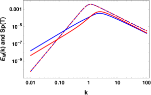
Figure 6: In this figure, magnetic field energy spectrum, $E_{\rm M}(k)$ (Dashed curves) and $\mbox{\rm Sp}(\mbox{\boldmath${\sf T}$}{})$ (Solid curves) for the helical and non helical case. The blue and red curves are for nonhelical and helical case respectively.

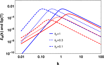
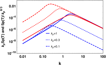
Figure 7: Left: Solutions for $\mbox{\rm Sp}(\mbox{\boldmath${\sf T}$}{})$ (red) for different $E_{\rm M}(k)$ (blue) for three values of $k_{\rm p}$. Right: solutions for $\mbox{\rm Sp}(\mbox{\boldmath${\sf T}$}{})$ scaled by $k_{\rm p}$ (blue) and $k_{\rm p}^{-8/3}$ (red), to see its scalings in the subinertial and inertial ranges, respectively.

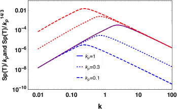
Figure 8: Similar to Fig. 7, but for a case with $\beta=1$. On the right, the solutions for $\mbox{\rm Sp}(\mbox{\boldmath${\sf T}$}{})$ are scaled by $k_{\rm p}$ (blue) and $k_{\rm p}^{14/3}$ (red), to see its scalings in the subinertial and inertial ranges, respectively. Violet indicates the two overlap for $k_{\rm p}=1$.

II.3 Overall behavior of the stress

At the most minimalistic level, we can say that the magnetic field shows an approximately self-similar evolution at late times, where for HEL, the peak value of $E_{\rm M}(k,t)$ is unchanged, but the position of the peak $k_{\rm p}$ goes to progressively smaller values as $k_{\rm p}\sim t^{-2/3}$.

To understand the consequences for the evolution of the stress, let us now consider an idealized model, where $E_{\rm M}(k)\equiv\mbox{\rm Sp}(\mathbf{B})/2$ has a $k^{4}$ subinertial range, where $k<k_{\rm p}$, with $k_{\rm p}(t)$ being the peak wave number, and a $k^{-5/3}$ inertial range spectrum for $k>k_{\rm p}$. The spectrum of the transverse traceless part of the stress, $\mbox{\rm Sp}(\mbox{\boldmath${\sf T}$}{})/2$, can be computed analytically using the expressions given in Appendix A (see Refs. Caprini et al. (2004); Sharma et al. (2020) for details) and is shown in Figs. 7 and 8 for the helical and nonhelical cases, respectively. In these figures, we take three instances where the magnetic peaks are at wave numbers $k_{\rm p}=1$, 0.3, and $0.1$.

For HEL, the position of the peak of $E_{\rm M}(k)$ is unchanged. We see that, in agreement with earlier work (Roper Pol et al., 2020a), the positions of the peak of $\mbox{\rm Sp}(\mbox{\boldmath${\sf T}$}{})$ are always at $2k_{\rm p}$. However, even though the peak values of $E_{\rm M}(k)$ are unchanged, except for the factor of two, those of $\mbox{\rm Sp}(\mbox{\boldmath${\sf T}$}{})$ are not and decay. Nevertheless, at small $k$, $\mbox{\rm Sp}(\mbox{\boldmath${\sf T}$}{})$ still increases proportional to $k_{\rm p}^{-1}$. If $k_{\rm p}\propto t^{-2/3}$, as expected for helical turbulence (Hatori, 1984; Biskamp and Müller, 1999; Brandenburg and Kahniashvili, 2017), we find that $\mbox{\rm Sp}(\mbox{\boldmath${\sf T}$}{})\propto t^{2/3}$ for small $k$.

For NHEL, as shown in Ref. Brandenburg and Kahniashvili (2017), the peak of the spectrum decreases with decreasing values of $k_{\rm p}$ proportional to $k_{\rm p}^{\beta}$, where $\beta$ is an exponent that can be between one and four. In Fig. 8, we present the case with $\beta=1$ and find that now $\mbox{\rm Sp}(\mbox{\boldmath${\sf T}$}{})(k)\propto k_{\rm p}$ for small $k$ and $\propto k_{\rm p}^{14/3}$ for large $k$. If $k_{\rm p}\propto t^{-1/2}$, as expected for the nonhelical case for $\beta=1$, $\mbox{\rm Sp}(\mbox{\boldmath${\sf T}$}{})\propto t^{-1/2}$ for small $k$. We have summarized the behavior of $\mbox{\rm Sp}(\mbox{\boldmath${\sf T}$}{})$ with time in Table LABEL:tildeT_vs_t for helical and nonhelical cases.

Table 2: Time evolution of $\mbox{\rm Sp}(\mbox{\boldmath${\sf T}$}{})$ and $|\tilde{T}|$ from theory

	helical	nonhelical
$\mbox{\rm Sp}(\mbox{\boldmath${\sf T}$}{})$ vs $k_{\rm p}$ at small $k$	$\propto 1/k_{\rm p}$	$\propto k_{\rm p}$
$k_{\rm p}$ vs $t$	$k_{\rm p}\propto t^{-2/3}$	$k_{\rm p}\propto t^{-1/2}$
$\mbox{\rm Sp}(\mbox{\boldmath${\sf T}$}{})$ vs $t$	$\mbox{\rm Sp}(\mbox{\boldmath${\sf T}$}{})\propto t^{2/3}$	$\mbox{\rm Sp}(\mbox{\boldmath${\sf T}$}{})\propto t^{-1/2}$
$|\tilde{T}|$ vs $t$	$|\tilde{T}|\propto t^{1/3}$	$|\tilde{T}|\propto t^{-1/4}$

Recently, it has been found that the Hosking integral Schekochihin (2020), a Saffman-like helicity integral, is well conserved in nonhelical magnetically dominated decaying turbulence (Hosking and Schekochihin, 2021; Zhou et al., 2022), which implies $\beta=1.5$. For the general case, we write $\mbox{\rm Sp}(\mbox{\boldmath${\sf T}$}{})\propto k_{\rm p}^{2\beta-1}$ (for $k<k_{\rm p}$), which implies $\mbox{\rm Sp}(\mbox{\boldmath${\sf T}$}{})\propto t^{-8/9}$ for $\beta=1.5$ and $k_{\rm p}\propto t^{-4/9}$.

It is also interesting to note that, for a given spectrum of the magnetic field, $\mbox{\rm Sp}(\mbox{\boldmath${\sf T}$}{})$ is different for HEL and NHEL; see the blue and red curves in Fig. 6), respectively. For the helical case, $\mbox{\rm Sp}(\mbox{\boldmath${\sf T}$}{})$ has smaller values compared to the nonhelical case at wave numbers below $k_{\rm p}$. However, it has large values for wave numbers around the peak and above. Such a feature of the stress spectrum also translates to the GW spectrum and that is why we see a difference in the final GW spectrum produced from helical and nonhelical cases discussed in the previous section.

III Predictions from algebraically growing stress

With the detailed information above, we are now in a position to compare with the predictions from a simple time-dependent model. In this section, we compute GW spectra by considering a simple model for the time evolution of the stress. It is assumed to increase algebraically as a power law characterized by a power law index $p$ during the time interval from $t=1$ to $t_{\rm e}$.

III.1 The model

We model the $+$ and $\times$ polarizations of the Fourier-transformed stress, $\tilde{T}(k,t)$, as

$$\tilde{T}(k,t)=\left\{\begin{array}[]{ll}|\tilde{T}_{0}(k)|\,t^{p},&1\leq t\leq t_{\rm e},\\ 0,&t>t_{\rm e},\end{array}\right.$$ (5)

where $|\tilde{T}_{0}(k)|$ represents $|\tilde{T}(k,t)|$ at the initial time and is obtained for given energy and helicity spectra of the magnetic field; see Appendix A for details. We note that the authors of Ref. Roper Pol et al. (2022a) have developed an analytical model for the GW spectrum on the basis of the time evolution of the stress, which they assumed constant during a certain interval – unlike our case. The authors explain the location of certain breaks in their GW spectrum as a consequence of the finite duration over which the stress is constant. This duration is an empirical input parameter. In our model, by contrast, the stress evolves as a power law with an index that is in principle known from MHD theory, although we can get even better agreement with the simulations when we take the actual power-law index that is realized in the simulations.

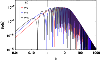
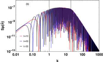
Figure 9: (a) $\mbox{\rm Sp}(\dot{\mbox{\boldmath${\sf h}$}{}}(k,t)$ at different times. Here, we assume $t=t_{\rm e}$, $E_{\rm M}=c(k/k_{\rm p})^{4}/(1+(k/k_{\rm p})^{17/3})$, where $k_{\rm p}=10$ and $c=10^{-4}$ and $p=-1/4$. The red, blue, and black curves are for $t_{\rm e}=2$, $4$, and $10$ respectively. The two black vertical lines correspond to $k_{*}$ and $2k_{\rm p}$. (b) $\mbox{\rm Sp}(\dot{\mbox{\boldmath${\sf h}$}{}})$ at times $t_{\rm e}=10$, $20$, and $30$.

To obtain the GW spectrum for our model, we first solve Eq. (4) for a case when the source is active during the interval $1<t<t_{\rm e}$ and thus obtain $\tilde{h}(k,t)$ and $\dot{\tilde{h}}(k,t)$. The solution for $t\geq t_{\rm e}$ is given by

$$\tilde{h}(k,t) =\int_{1}^{t}\frac{\sin k(t-t^{\prime})}{k}\,\frac{6\tilde{T}(k,t^{\prime})}{t^{\prime}}\,dt^{\prime},$$ (6)

$$\dot{\tilde{h}}(k,t) =\int_{1}^{t}\cos k(t-t^{\prime})\,\frac{6\tilde{T}(k,t^{\prime})}{t^{\prime}}\,dt^{\prime}.$$ (7)

Using Eq. (7) and our model for $\tilde{T}(k,t)$, we obtain

$$\dot{\tilde{h}}(k,t) =\frac{-3|\tilde{T}_{0}(k)|}{(kt_{0})^{p}}\Big{\{}e^{i(kt-p\pi/2)}\big{[}\Gamma(p,ikt_{\rm e})-\Gamma(p,ikt_{0})\big{]}$$

$$+e^{-i(kt-p\pi/2)}\big{[}\Gamma(p,-ikt_{\rm e})-\Gamma(p,-ikt_{0})\big{]}\Big{\}}.$$ (8)

In the above expression, $t_{0}=1$ represents the initial time. In Fig. 9(a), we show $\mbox{\rm Sp}(\dot{\mbox{\boldmath${\sf h}$}{}})$ at different times for this model with $p=-1/4$. The red, blue, and black curves represent $\mbox{\rm Sp}(\dot{\mbox{\boldmath${\sf h}$}{}})$ at $t=2$, $4$, and $10$, respectively. It is evident from this figure that $\mbox{\rm Sp}(\dot{\mbox{\boldmath${\sf h}$}{}})$ is almost flat for $1\mathrel{\mathchoice{\vbox{\offinterlineskip\halign{\hfil$\displaystyle#$\hfil\cr<\cr\sim\cr}}}{\vbox{\offinterlineskip\halign{\hfil$\textstyle#$\hfil\cr<\cr\sim\cr}}}{\vbox{\offinterlineskip\halign{\hfil$\scriptstyle#$\hfil\cr<\cr\sim\cr}}}{\vbox{\offinterlineskip\halign{\hfil$\scriptscriptstyle#$\hfil\cr<\cr\sim\cr}}}}k\mathrel{\mathchoice{\vbox{\offinterlineskip\halign{\hfil$\displaystyle#$\hfil\cr<\cr\sim\cr}}}{\vbox{\offinterlineskip\halign{\hfil$\textstyle#$\hfil\cr<\cr\sim\cr}}}{\vbox{\offinterlineskip\halign{\hfil$\scriptstyle#$\hfil\cr<\cr\sim\cr}}}{\vbox{\offinterlineskip\halign{\hfil$\scriptscriptstyle#$\hfil\cr<\cr\sim\cr}}}}2k_{\rm p}$ and declines as $\propto k^{-11/3}$ for $k>2k_{\rm p}$. $\mbox{\rm Sp}(\dot{\mbox{\boldmath${\sf h}$}{}})$ is proportional to $k^{2}$ for $k<k_{\rm H}$, where $k_{\rm H}$ represents the wave number corresponding to the Hubble horizon size at $t=t_{\rm e}$. Further, as time increases, $\mbox{\rm Sp}(\dot{\mbox{\boldmath${\sf h}$}{}})$ at low wave numbers ($k_{\rm H}<k<1$) grows and saturates, as is evident from Fig. 9(b).

To understand the role of the power-law index in the algebraically growing part of the stress on $\mbox{\rm Sp}(\dot{\mbox{\boldmath${\sf h}$}{}})$, we calculate $\mbox{\rm Sp}(\dot{\mbox{\boldmath${\sf h}$}{}})$ for different values of $p$. Those are shown in the right-hand panel of Fig. 10. Here, $\mbox{\rm Sp}(\dot{\mbox{\boldmath${\sf h}$}{}})$ is rapidly oscillating, so we plot in this figure only its envelope. From this figure, we conclude that $\mbox{\rm Sp}(\dot{\mbox{\boldmath${\sf h}$}{}})$ can be divided into three regime. We begin discussing first the high wave number regime ($k>k_{0}$, regime I), where $k_{0}$ represents the wave number corresponding to the Hubble horizon at the initial time. $\mbox{\rm Sp}(\dot{\mbox{\boldmath${\sf h}$}{}})$ is flat and changes to $k^{-11/3}$ for $k>2k_{\rm p}$. For very low wave numbers corresponding to the superhorizon range ($k<k_{\rm H}$, regime III) $\mbox{\rm Sp}(\dot{\mbox{\boldmath${\sf h}$}{}})$ is proportional to $k^{2}$. In the intermediate regime [$k_{\rm H}\lesssim k\lesssim(1-p)/t_{0}$, regime II], $\mbox{\rm Sp}(\dot{\mbox{\boldmath${\sf h}$}{}})$ changes from a flat spectrum to a $k^{2}$ spectrum as the wave number decreases. Note that, as the wave numbers decrease, the transition from a flat spectrum to a $k^{2}$ spectrum is faster for the case when $p=-1/4$ than when it is $p=1/3$. The wave number at which this transition occurs depends on the value of $p$ and can be understood as follows. In the algebraically growing phase, the typical time scale over which $\tilde{T}/t$ decays, is $\delta t_{T}\sim t/(1-p)$ and the typical time scale for sourcing GWs at a given wave number $k$ just after $t=1$ is $\delta t_{\rm GW}\sim 1/k$, as can be inferred from the cosine function in Eq. (7). The value of $\tilde{T}/t$ does not change much when $\delta t_{\rm GW}/\delta t_{T}\leq 1$. This implies that, for $k>(1-p)/t_{0}$, there will be a finite interval during which $\tilde{T}/t$ can be assumed constant. However, for $k<(1-p)/t_{0}$, $\tilde{T}/t$ always changes. The wave number $k\sim(1-p)/t_{0}$ corresponds to the wave number where $\mbox{\rm Sp}(\dot{\mbox{\boldmath${\sf h}$}{}})$ starts changing from a flat spectrum.

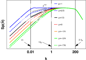
Figure 10: $\mbox{\rm Sp}(\dot{\mbox{\boldmath${\sf h}$}{}})$ for different values of $p$. Here, the left, middle, and right black vertical lines represent the wave numbers corresponding to the horizon size at the final time $t$, the initial time $t_{0}=1$, and $2k_{\rm p}$, respectively.

The nature of $\mbox{\rm Sp}(\dot{\mbox{\boldmath${\sf h}$}{}})$ can also be understood by writing the expression of $\dot{\tilde{h}}(k,t)$, given in Eq. (8), for different limits depending on the values of $kt_{0}$ and $kt_{\rm e}$. For $t_{\rm e}\gg t_{0}$, which is indeed the case, and $p<1$, Eq. (8) reduces to

$$\frac{\dot{\tilde{h}}(k,t)}{6|\tilde{T}_{0}(k)|}\approx\left\{\begin{array}[]{lr}\frac{\sin{k(t-t_{0})}}{kt_{0}}\quad\text{(I)},\\[5.0pt] \frac{\Gamma[p]}{(kt_{0})^{p}}\cos\left({kt-\frac{p\pi}{2}}\right)-\frac{\cos{kt}}{p}\quad\text{(II)},\\[5.0pt] \frac{\cos{kt}}{p}\left[\left(\frac{t_{\rm e}}{t_{0}}\right)^{p}-1\right]\quad\text{(III)}.\end{array}\right.$$ (9)

Using this, we calculate the spectrum of $\dot{\tilde{h}}$; it is given by

$$\frac{\mbox{\rm Sp}(\dot{\mbox{\boldmath${\sf h}$}{}})(k,t)}{36|\tilde{T}_{0}(k)|^{2}}\approx\left\{\begin{array}[]{lr}\left[\frac{\sin{k(t-t_{0})}}{t_{0}}\right]^{2}\quad\text{(I)},\\[5.0pt] k^{2}\Big{[}-\frac{\cos{kt}}{p}+\frac{\Gamma[p]}{(kt_{0})^{p}}\cos({kt-\frac{p\pi}{2}})\Big{]}^{2}\,\text{(II)},\\[5.0pt] k^{2}\Big{\{}\frac{\cos{kt}}{p}\left[\left(\frac{t_{\rm e}}{t_{0}}\right)^{p}-1\right]\Big{\}}^{2}\quad\text{(III)}.\end{array}\right.$$ (10)

From the above expression, we conclude that the break points for the different slopes of $\mbox{\rm Sp}(\dot{\mbox{\boldmath${\sf h}$}{}})$ is decided by $|\tilde{T}_{0}(k)|^{2}$ for $k>t_{0}^{-1}$. Here, $|\tilde{T}_{0}(k)|^{2}$ is flat for $k<2k_{\rm p}$ and proportional to $k^{-11/3}$ for $k>2k_{\rm p}$. For the superhorizon modes, i.e., $k<1/t_{\rm e}$, $\mbox{\rm Sp}(\dot{\mbox{\boldmath${\sf h}$}{}})$ is proportional to $k^{2}$, and for wave numbers $t_{0}^{-1}<k<t_{\rm e}^{-1}$, $\mbox{\rm Sp}(\dot{\mbox{\boldmath${\sf h}$}{}})$ changes from a flat spectrum to $k^{2}$, as shown as the blue curves in Fig. 10.

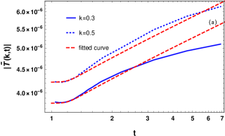
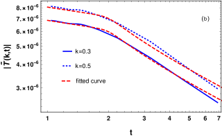
Figure 11: $\tilde{T}(k,t)$ vs. $t$. (a) The solid and dotted blue curves correspond to the time evolution of $\tilde{T}(k,t)$ vs $t$ obtained from the simulation for $k=0.3$ and $0.5$, respectively, for HEL and the red curve corresponds to a broken power law fit to the blue curves. (b) Same as (a), but for NHEL.

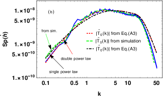
Figure 12: $\mbox{\rm Sp}(\dot{\mbox{\boldmath${\sf h}$}{}})$ vs $k$: (a) The solid blue curve represents $\mbox{\rm Sp}(\dot{\mbox{\boldmath${\sf h}$}{}})$ corresponding to the run shown in Fig. 1, respectively. The dotted red and dashed green curves represent the spectra obtained in the model for the time evolution of $\tilde{T}(k,t)$ given in column 2 of Table LABEL:table2. The dot dashed black curve represents $\mbox{\rm Sp}(\dot{\mbox{\boldmath${\sf h}$}{}})$ for the time evolution of $\tilde{T}(k,t)$ given in column 1 of Table LABEL:table2. The red curves are for the case when $|\tilde{T}_{0}(k)|$ is obtained using Eq. (A) of Appendix A. For the green curves, $|\tilde{T}_{0}(k)|$ is taken from the simulation. (b) Same as (a), but for nonhelical case.

In this model, we take the same algebraic evolution with a constant power-law index for all wave numbers. In general, however, the time evolution of $\tilde{T}(k,t)$ is different for wave numbers below and above the peak of $\mbox{\rm Sp}(\mbox{\boldmath${\sf T}$}{})(k,t)$. For the case of helical magnetic fields discussed in Fig. 7, the value of $\mbox{\rm Sp}(\mbox{\boldmath${\sf T}$}{})$ for a particular $k<2k_{\rm p}$ at the initial time, grows as $t^{2/3}$ until the time for which $\mbox{\rm Sp}(\mbox{\boldmath${\sf T}$}{})$ peaks at this particular wave number. After this time, the value of $\mbox{\rm Sp}(\mbox{\boldmath${\sf T}$}{})$ for this particular $k$ starts decreasing as $t^{-16/9}$. This implies that we would have assumed $\tilde{T}(k)\propto t^{1/3}$ for $k<k_{\rm p}$ and $\tilde{T}(k)\propto t^{-8/9}$ for $k>k_{\rm p}$. For the nonhelical magnetic field shown in Fig. 8, $\mbox{\rm Sp}(\mbox{\boldmath${\sf T}$}{})$ is always decreasing. For $k<2k_{\rm p}$ at the initial time, it first decreases as $t^{-1/2}$ and later switches to $t^{-7/3}$. We study $\mbox{\rm Sp}(\dot{\mbox{\boldmath${\sf h}$}{}})$ by incorporating this and find that there is no difference in the final $\mbox{\rm Sp}(\dot{\mbox{\boldmath${\sf h}$}{}})$ compared to the one obtained in our model. This is why we did not consider the aforementioned evolution of the stress to keep the model simple.

IV Comparison of the analytical model with simulation results

In the above section, we discussed $\mbox{\rm Sp}(\dot{\mbox{\boldmath${\sf h}$}{}})$ in a model inspired by the fact that the GW spectrum does not change if we change the stress tensor by its modulus for decaying MHD turbulence in the early Universe. In this model, we approximate the stress tensor by $|\tilde{T}(k,t)|\equiv\sqrt{\mbox{\rm Sp}(\mbox{\boldmath${\sf T}$}{})/4\pi k^{2}}$ and its time evolution is parameterized as a power law with index $p$; see Fig. 11. In this section, we provide a comparison for $\mbox{\rm Sp}(\dot{\mbox{\boldmath${\sf h}$}{}})$ obtained in this model with the simulation results discussed in Section II.2. To compare, we show $\mbox{\rm Sp}(\dot{\mbox{\boldmath${\sf h}$}{}})$ obtained from the model and different simulations together. In Figs. 12(a) and (b), we plot the spectra for the runs shown in Figs. 1 and 2 and discussed in Section II.2. For the dotted-dashed black curve, $|\tilde{T}_{0}(k)|$ is obtained by using Eq. (A) of Appendix A, where we take $E_{\rm M}=c(k/k_{\rm p})^{4}/[1+(k/k_{\rm p})^{17/3}]$ and the value of the constant $c$ is determined such that the obtained stress spectrum matches with that of the simulation at $t=1$. For this case, the stress spectrum evolution is modeled as a single power law and the value of $p$ is $1/3$ and $-1/4$ for the helical and nonhelical cases, respectively. The value of $p$ is decided from the time evolution of the low wave number tail of $\mbox{\rm Sp}(\mbox{\boldmath${\sf T}$}{})$, as discussed in Section II.3. From this figure, it is concluded that the spectral nature of $\mbox{\rm Sp}(\dot{\mbox{\boldmath${\sf h}$}{}})$ matches well with the prediction from the model. However, there is a difference at small wave numbers, especially for the nonhelical case. This is due to the fact that the modelling of $\mbox{\rm Sp}(\mbox{\boldmath${\sf T}$}{})$ by a single power does not provide a better fit to the evolution obtained in NHEL.

A double power law of the form $t^{-1/3}/[1+(t-1)^{n}]^{5/7n}$, where $n$ regulates the transition, here with $n=10$, provides a better fit to $\mbox{\rm Sp}(\mbox{\boldmath${\sf T}$}{})$ for the low frequency tail for NHEL; see Fig. 11. In this figure, we plot $\tilde{T}(k,t)$ obtained from the simulation in solid and dotted blue for the wave numbers $k=0.3$ and $0.5$, respectively and the double power law fit to the blue curves is in dashed red color. The double power law, which fits $\tilde{T}(k,t)$ for HEL, is $1/[1+(t-0.2)^{n}]^{5/24n}$, where $n=20$. After considering such a time evolution, the obtained $\mbox{\rm Sp}(\dot{\mbox{\boldmath${\sf h}$}{}})$ is shown as the dotted red curve in Fig. 12(b). For the dashed green curve, we consider $|\tilde{T}_{0}(k)|=\sqrt{\mbox{\rm Sp}(\mbox{\boldmath${\sf T}$}{})/4\pi k^{2}}$ and $\mbox{\rm Sp}(\mbox{\boldmath${\sf T}$}{})$ is obtained from the simulation at $t=1$. These different forms of the time evolution of $\tilde{T}(k,t)$ are given in Table LABEL:table2. The spectra in Figs. 12(a) and (b) are plotted at a time when the value of the $\mbox{\rm Sp}(\dot{\mbox{\boldmath${\sf h}$}{}})$ for each wave number has reached approximately a constant value. The actual time for HEL is $t=175.5$ and for NHEL it is $t=99.5$. For earlier times, the mean value of $\mbox{\rm Sp}(\dot{\mbox{\boldmath${\sf h}$}{}})$ is in reasonably good agreement with the values obtained from the model.

We notice that the nature of the GW spectra in HEL and NHEL are different. There is large power in HEL compared to NHEL around the peak of the GW spectrum for the same strength of the initial magnetic field. This is due to the presence of an additional term due to the helicity spectrum in the stress spectrum; see Appendix A.

Table 3: Time dependence of $\tilde{T}(k,t)$ taken in our analysis

run	from theory	from simulation
hel	$\left(\frac{t}{t_{0}}\right)^{1/3}$	$\frac{1}{(1+(t-0.2)^{n})^{5/24n}}$
nonhel	$\left(\frac{t}{t_{0}}\right)^{-1/4}$	$\frac{t^{-1/6}}{(1+(t-1)^{n})^{5/14n}}$

V Conclusions

In this work, we have suggested a simple model to understand the GW spectrum obtained for decaying MHD turbulence in the early Universe. The Fourier-transformed stress is taken to be $|\tilde{T}(k,t)|$, i.e., we ignore changes in the phase, and its time evolution is parameterized by a power law. Such a time evolution of the stress is motivated by the simulations for the decaying MHD turbulence at low wave numbers discussed in Section II.2. We find that the spectral nature of the GW spectrum is well represented by this simple model. In this work, we also show that the nature of the GW spectra in the helical case are different from those in the nonhelical case. Apart from the polarization of GW, this spectral difference may also be important in distinguishing the helical and nonhelical nature of the primordial magnetic field.

In this work, we have developed a model to understand the low frequency tail of the GW spectrum in the cases where turbulence is initiated suddenly. However, it will now also be interesting to study cases where the magnetic field is generated selfconsistently, such as through the chiral magnetic effect in the early Universe (Rogachevskii et al., 2017; Schober et al., 2018). It would be interesting to see if a model such as the one discussed in this paper can also explain the GW spectra obtained through the chiral magnetic effect. This, we hope to report in a future study.

Data availability—The source code used for the simulations of this study, the Pencil Code, is freely available from Refs. Pencil Code Collaboration et al. (2021). Supplemental Material with plots similar to Figs. 3 and 4, but for other wave vectors of the same length, along with the simulation setups and the corresponding data are freely available from Ref. Sharma and Brandenburg .

Appendix A $\mbox{\rm Sp}(\mbox{\boldmath${\sf T}$}{})$ in terms of magnetic spectrum

Here, we provide the expressions for the stress spectrum in terms of the magnetic spectrum for helical and nonhelical cases; see Refs. Caprini et al. (2004) and Sharma et al. (2020) for the derivation. The two-point correlation for the nonhelical magnetic field in Fourier space is given by,

$$\langle\tilde{B}_{i}(\mathbf{k})\tilde{B}^{*}_{j}(\mathbf{k}^{\prime})\rangle =(2\pi)^{3}\delta(\mathbf{k}-\mathbf{k}^{\prime})(\delta_{ij}-\hat{\mathbf{k}}_{i}\hat{\mathbf{k}}_{j})P_{\rm SM}(k)$$ (11)

Assuming a Gaussian nature of the magnetic field fluctuations, the stress spectrum is given by

$$\mbox{\rm Sp}(\mbox{\boldmath${\sf T}$}{})\equiv 4\pi k^{2}\langle\tilde{T}_{ij}^{\rm TT}(\mathbf{k})\tilde{T}_{*ij}^{\rm TT}(\mathbf{k})\rangle=4\pi k^{2}\int d^{3}q\Big{[}P_{\rm SM}(q)$$

$$P_{\rm SM}({|\mathbf{k}-\mathbf{q}|})(1+\gamma^{2}+\beta^{2}+\gamma^{2}\beta^{2})\Big{]}.$$ (12)

Here, $\tilde{T}_{ij}^{\rm TT}(\mathbf{k})=-B_{i}B_{j}+\frac{1}{2}\delta_{ij}B_{k}B_{k}$. In terms of the energy spectrum, $E_{\rm M}(k)\equiv 4\pi k^{2}P_{\rm SM}(k)$, the above expression reduces to

$$\mbox{\rm Sp}(\mbox{\boldmath${\sf T}$}{}) =\frac{1}{4\pi}\int d^{3}q\frac{k^{2}}{q^{2}|\mathbf{k}-\mathbf{q}|^{2}}\Big{[}E_{\rm M}(q)$$

$$E_{\rm M}({|\mathbf{k}-\mathbf{q}|})(1+\gamma^{2}+\beta^{2}+\gamma^{2}\beta^{2})\Big{]}.$$ (13)

In the above expressions $\gamma=\hat{\mathbf{k}}\cdot\hat{\mathbf{q}}$ and $\beta=\hat{\mathbf{k}}\cdot\widehat{\mathbf{k}-\mathbf{q}}$. For helical magnetic fields, there is an additional antisymmetric contribution to the two-point correlation and is given by,

$$\langle\tilde{B}_{i}(\mathbf{k})\tilde{B}^{*}_{j}(\mathbf{k}^{\prime})\rangle =(2\pi)^{3}\delta(\mathbf{k}-\mathbf{k}^{\prime})\Big{(}(\delta_{ij}-\hat{\mathbf{k}}_{i}\hat{\mathbf{k}}_{j})P_{\rm SM}(k)$$

$$+i\epsilon_{ijm}\hat{\mathbf{k}}_{m}P_{AM}(k)\Big{)}.$$ (14)

The stress spectrum for this case is given by

$$\mbox{\rm Sp}(\mbox{\boldmath${\sf T}$}{})= 4\pi k^{2}\int d^{3}q\Big{[}P_{\rm SM}(\mathbf{q})P_{\rm SM}({|\mathbf{k}-\mathbf{q}|})(1+\gamma^{2}+\beta^{2}+\gamma^{2}\beta^{2})$$

$$+4\gamma\beta P_{\rm AM}(q)P_{\rm AM}({|\mathbf{k}-\mathbf{q}|})\Big{]}.$$ (15)

In terms of the energy spectrum, $E_{\rm M}(k)$, and the helicity spectrum, $H_{M}(k)\equiv 4\pi k^{2}P_{\rm AM}(k)$, the above expression reduces to

$$\mbox{\rm Sp}(\mbox{\boldmath${\sf T}$}{})= \frac{1}{4\pi}\int d^{3}q\frac{k^{2}}{q^{2}|\mathbf{k}-\mathbf{q}|^{2}}\Big{[}E_{\rm M}(\mathbf{q})E_{\rm M}({|\mathbf{k}-\mathbf{q}|})$$

$$(1+\gamma^{2}+\beta^{2}+\gamma^{2}\beta^{2})+4\gamma\beta H_{M}(q)H_{M}({|\mathbf{k}-\mathbf{q}|})\Big{]}.$$ (16)

References

- Kamionkowski et al. (1994) M. Kamionkowski, A. Kosowsky, and M. S. Turner, Phys. Rev. D 49, 2837 (1994), arXiv:astro-ph/9310044 [astro-ph] .
- Hogan (2000) C. J. Hogan, Phys. Rev. Lett. 85, 2044 (2000).
- Kosowsky et al. (2002) A. Kosowsky, A. Mack, and T. Kahniashvili, Phys. Rev. D 66, 024030 (2002), arXiv:astro-ph/0111483 [astro-ph] .
- Dolgov et al. (2002) A. D. Dolgov, D. Grasso, and A. Nicolis, Phys. Rev. D 66, 103505 (2002), arXiv:astro-ph/0206461 [astro-ph] .
- Caprini and Figueroa (2018) C. Caprini and D. G. Figueroa, CQGra 35, 163001 (2018), arXiv:1801.04268 [astro-ph.CO] .
- Kajantie et al. (1996) K. Kajantie, M. Laine, K. Rummukainen, and M. Shaposhnikov, Phys. Rev. Lett. 77, 2887 (1996).
- Aoki et al. (2006) Y. Aoki, G. EndrHodi, Z. Fodor, S. D. Katz, and K. K. Szabó, Nature (London) 443, 675 (2006), arXiv:hep-lat/0611014 [hep-lat] .
- Witten (1984) E. Witten, Phys. Rev. D 30, 272 (1984).
- Hogan (1986) C. J. Hogan, Mon. Not. Roy. Astron. Soc. 218, 629 (1986).
- Mazumdar and White (2019) A. Mazumdar and G. White, Rep. Prog. Phys. 82, 076901 (2019).
- Hindmarsh et al. (2021) M. Hindmarsh, M. Lüben, J. Lumma, and M. Pauly, SciPost Phys. Lect. Notes , 24 (2021).
- Turner and Widrow (1988) M. S. Turner and L. M. Widrow, Phys. Rev. D 37, 2743 (1988).
- Vachaspati (1991) T. Vachaspati, PhLB 265, 258 (1991).
- Ratra (1992) B. Ratra, Astrophys. J. Lett. 391, L1 (1992).
- Durrer and Neronov (2013) R. Durrer and A. Neronov, Astron. Astrophys. Rev. 21, 62 (2013), arXiv:1303.7121 [astro-ph.CO] .
- Subramanian (2016) K. Subramanian, Rep. Prog. Phys. 79, 076901 (2016).
- Subramanian (2019) K. Subramanian, Galaxies 7, 47 (2019), arXiv:1903.03744 [astro-ph.CO] .
- Vachaspati (2021) T. Vachaspati, Reports on Progress in Physics 84, 074901 (2021), arXiv:2010.10525 [astro-ph.CO] .
- Brandenburg et al. (2021) A. Brandenburg, Y. He, and R. Sharma, Astrophys. J. 922, 192 (2021), arXiv:2107.12333 [astro-ph.CO] .
- Arzoumanian et al. (2020) Z. Arzoumanian et al. (NANOGrav), Astrophys. J. Lett. 905, L34 (2020), arXiv:2009.04496 [astro-ph.HE] .
- Goncharov et al. (2021) B. Goncharov et al., Astrophys. J. Lett. 917, L19 (2021), arXiv:2107.12112 [astro-ph.HE] .
- Chen et al. (2021) S. Chen et al., Mon. Not. Roy. Astron. Soc. 508, 4970 (2021), arXiv:2110.13184 [astro-ph.HE] .
- Antoniadis et al. (2022) J. Antoniadis et al., Mon. Not. Roy. Astron. Soc. 510, 4873 (2022), arXiv:2201.03980 [astro-ph.HE] .
- Neronov et al. (2021) A. Neronov, A. Roper Pol, C. Caprini, and D. Semikoz, Phys. Rev. D 103, L041302 (2021).
- Sharma (2022) R. Sharma, Phys. Rev. D 105, L041302 (2022), arXiv:2102.09358 [astro-ph.CO] .
- Roper Pol et al. (2022a) A. Roper Pol, C. Caprini, A. Neronov, and D. Semikoz, Phys. Rev. D 105, 123502 (2022a), arXiv:2201.05630 [astro-ph.CO] .
- Hellings and Downs (1983) R. W. Hellings and G. S. Downs, Astrophys. J. Lett. 265, L39 (1983).
- Roper Pol et al. (2020a) A. Roper Pol, S. Mandal, A. Brandenburg, T. Kahniashvili, and A. Kosowsky, Phys. Rev. D 102, 083512 (2020a), arXiv:1903.08585 [astro-ph.CO] .
- Auclair et al. (2022) P. Auclair, C. Caprini, D. Cutting, M. Hindmarsh, K. Rummukainen, D. A. Steer, and D. J. Weir, (2022), arXiv:2205.02588 [astro-ph.CO] .
- Brandenburg et al. (2015) A. Brandenburg, T. Kahniashvili, and A. G. Tevzadze, PhRvL 114, 075001 (2015), arXiv:1404.2238 .
- Zrake (2014) J. Zrake, Astrophys. J. Lett. 794, L26 (2014), arXiv:1407.5626 [astro-ph.HE] .
- Kosowsky et al. (2002) A. Kosowsky, A. Mack, and T. Kahniashvili, PhRvD 66, 024030 (2002).
- Gogoberidze et al. (2007) G. Gogoberidze, T. Kahniashvili, and A. Kosowsky, Phys. Rev. D 76, 083002 (2007), arXiv:0705.1733 [astro-ph] .
- Kahniashvili et al. (2008) T. Kahniashvili, A. Kosowsky, G. Gogoberidze, and Y. Maravin, PhRvD 78, 043003 (2008).
- Caprini et al. (2009) C. Caprini, R. Durrer, and G. Servant, J. Cosmol. Astropart. Phys. 2009, 024 (2009), arXiv:0909.0622 [astro-ph.CO] .
- Niksa et al. (2018) P. Niksa, M. Schlederer, and G. Sigl, Class. Quant. Grav. 35, 144001 (2018), arXiv:1803.02271 [astro-ph.CO] .
- Sharma et al. (2020) R. Sharma, K. Subramanian, and T. R. Seshadri, Phys. Rev. D 101, 103526 (2020), arXiv:1912.12089 [astro-ph.CO] .
- Roper Pol et al. (2022b) A. Roper Pol, S. Mandal, A. Brandenburg, and T. Kahniashvili, J. Cosmol. Astropart. Phys. 2022, 019 (2022b), arXiv:2107.05356 [gr-qc] .
- Kahniashvili et al. (2021) T. Kahniashvili, A. Brandenburg, G. Gogoberidze, S. Mandal, and A. R. Pol, PhRvR 3, 013193 (2021), arXiv:2011.05556 [astro-ph.CO] .
- Dahl et al. (2021) J. Dahl, M. Hindmarsh, K. Rummukainen, and D. Weir, arXiv e-prints , arXiv:2112.12013 (2021), arXiv:2112.12013 [gr-qc] .
- Roper Pol et al. (2020b) A. Roper Pol, A. Brandenburg, T. Kahniashvili, A. Kosowsky, and S. Mandal, GApFD 114, 130 (2020b).
- Brandenburg et al. (1996) A. Brandenburg, K. Enqvist, and P. Olesen, Phys. Rev. D 54, 1291 (1996), arXiv:astro-ph/9602031 [astro-ph] .
- Brandenburg et al. (2017) A. Brandenburg, T. Kahniashvili, S. Mandal, A. Roper Pol, A. G. Tevzadze, and T. Vachaspati, Phys. Rev. D 96, 123528 (2017).
- (44) R. Sharma and A. Brandenburg, Supplemental Material and Datasets for Low frequency tail of gravitational wave spectra from hydromagnetic turbulence, doi:10.5281/zenodo.7014823 (v2022.08.22); see also http://norlx65.nordita.org/~brandenb/projects/LowFreqTail/ for easier access 10.5281/zenodo.7014823.
- Caprini et al. (2004) C. Caprini, R. Durrer, and T. Kahniashvili, Phys. Rev. D 69, 063006 (2004), arXiv:astro-ph/0304556 [astro-ph] .
- Hatori (1984) T. Hatori, JPSJ 53, 2539 (1984).
- Biskamp and Müller (1999) D. Biskamp and W.-C. Müller, Phys. Rev. Lett. 83, 2195 (1999), arXiv:physics/9903028 [physics.flu-dyn] .
- Brandenburg and Kahniashvili (2017) A. Brandenburg and T. Kahniashvili, PhRvL 118, 055102 (2017), arXiv:1607.01360 [physics.flu-dyn] .
- Schekochihin (2020) A. A. Schekochihin, arXiv e-prints , arXiv:2010.00699 (2020), arXiv:2010.00699 [physics.plasm-ph] .
- Hosking and Schekochihin (2021) D. N. Hosking and A. A. Schekochihin, Phys. Rev. X 11, 041005 (2021).
- Zhou et al. (2022) H. Zhou, R. Sharma, and A. Brandenburg, arXiv e-prints , arXiv:2206.07513 (2022), arXiv:2206.07513 [physics.plasm-ph] .
- Rogachevskii et al. (2017) I. Rogachevskii, O. Ruchayskiy, A. Boyarsky, J. Fröhlich, N. Kleeorin, A. Brandenburg, and J. Schober, Astrophys. J. 846, 153 (2017), arXiv:1705.00378 [physics.plasm-ph] .
- Schober et al. (2018) J. Schober, I. Rogachevskii, A. Brandenburg, A. Boyarsky, J. Fröhlich, O. Ruchayskiy, and N. Kleeorin, Astrophys. J. 858, 124 (2018).
- Pencil Code Collaboration et al. (2021) Pencil Code Collaboration, A. Brandenburg, A. Johansen, P. Bourdin, W. Dobler, W. Lyra, M. Rheinhardt, S. Bingert, N. Haugen, A. Mee, F. Gent, N. Babkovskaia, C.-C. Yang, T. Heinemann, B. Dintrans, D. Mitra, S. Candelaresi, J. Warnecke, P. Käpylä, A. Schreiber, P. Chatterjee, M. Käpylä, X.-Y. Li, J. Krüger, J. Aarnes, G. Sarson, J. Oishi, J. Schober, R. Plasson, C. Sandin, E. Karchniwy, L. Rodrigues, A. Hubbard, G. Guerrero, A. Snodin, I. Losada, J. Pekkilä, and C. Qian, JOSS 6, 2807 (2021).