Laminar and turbulent dynamos in chiral magnetohydrodynamics-I: Theory

Abstract

The magnetohydrodynamic (MHD) description of plasmas with relativistic particles necessarily includes an additional new field, the chiral chemical potential associated with the axial charge (i.e., the number difference between right- and left-handed relativistic fermions). This chiral chemical potential gives rise to a contribution to the electric current density of the plasma (chiral magnetic effect). We present a self-consistent treatment of the chiral MHD equations, which include the back-reaction of the magnetic field on a chiral chemical potential and its interaction with the plasma velocity field. A number of novel phenomena are exhibited. First, we show that the chiral magnetic effect decreases the frequency of the Alfvén wave for incompressible flows, increases the frequencies of the Alfvén wave and of the fast magnetosonic wave for compressible flows, and decreases the frequency of the slow magnetosonic wave. Second, we show that, in addition to the well-known laminar chiral dynamo effect, which is not related to fluid motions, there is a dynamo caused by the joint action of velocity shear and chiral magnetic effect. In the presence of turbulence with vanishing mean kinetic helicity, the derived mean-field chiral MHD equations describe turbulent large-scale dynamos caused by the chiral alpha effect, which is dominant for large fluid and magnetic Reynolds numbers. The chiral alpha effect is due to an interaction of the chiral magnetic effect and fluctuations of the small-scale current produced by tangling magnetic fluctuations (which are generated by tangling of the large-scale magnetic field by sheared velocity fluctuations). These dynamo effects may have interesting consequences in the dynamics of the early universe, neutron stars, and the quark–gluon plasma.

1. Introduction

Hydrodynamics is a universal description of a vast variety of systems ranging from astrophysical environments to biological systems. A hydrodynamic description is possible whenever a form of local thermal equilibrium prevails in macroscopically large regions of space. Variables describing the thermodynamic state (temperature $T$, chemical potentials $\mu_{i}$ conjugate to conserved charges) become state functions ($T\to T(t,\bm{x})$, $\mu_{i}\to\mu_{i}(t,\bm{x})$, etc.) that depend on space and time. Their evolution equations, which involve to the flow velocity, $\bm{U}(t,\bm{x})$, of the plasma or fluid, follow from energy–momentum and charge conservation (Landau & Lifshitz, 1959, Chapter 15).

Details of the microscopic physics are encoded in kinetic coefficients (viscosity, diffusion coefficient, conductivities, etc.). Most hydrodynamical systems are “agnostic” about the quantum nature of the microscopic degrees of freedom. Situations where quantum physics affects the hydrodynamical description of the macroscopic systems are rare. Superfluidity (Landau & Lifshitz, 1959, Chapter 16) is a prominent example of a phenomenon where the quantum nature of the underlying particles drastically changes the properties of the fluid at macroscopic scales.

Two decades ago, a novel phenomenon tied to quantum physics was identified (see, e.g., Kharzeev, 2011; Kharzeev et al., 2013; Zakharov, 2013; Giovannini, 2013; Kharzeev, 2014; Miransky & Shovkovy, 2015; Kharzeev et al., 2016). The hydrodynamical description of magnetized systems of relativistic fermions in weakly coupled plasmas (Alekseev et al., 1998; Giovannini, 2013), of quasi-particles in new materials such as graphene (Miransky & Shovkovy, 2015), and of the quark–gluon plasma (Kharzeev et al., 2016) cannot be formulated in terms of only the standard magnetohydrodynamic (MHD) variables (flow velocity $\bm{U}$, magnetic field $\bm{B}$, density of plasma $\rho$, and pressure $p$) appearing in the Navier-Stokes and the Maxwell equations. The hydrodynamics of a chiral plasma necessarily contains an additional degree of freedom corresponding to a spacetime-dependent chemical potential, conjugated to the number difference between right-chiral and left-chiral fermions. The dynamics of this degree of freedom is coupled to the magnetic helicity.

Many new effects arise, among which the most notable one is the chiral magnetic effect (CME), namely the presence of a contribution to the electric current parallel to the magnetic field. This effect has first been described by Vilenkin (1980) and rederived later using different arguments (see, e.g., Redlich & Wijewardhana, 1985; Tsokos, 1985; Alekseev et al., 1998; Fröhlich & Pedrini, 2000, 2002; Fukushima et al., 2008; Son & Surowka, 2009). This contribution to the electric current causes an instability in the system (Joyce & Shaposhnikov, 1997) that has been analyzed in many works (Fröhlich & Pedrini, 2000; Ooguri & Oshikawa, 2012; Boyarsky et al., 2012a; Kumar et al., 2014; Grabowska et al., 2015; Manuel & Torres-Rincon, 2015; Buividovich & Ulybyshev, 2016; Boyarsky et al., 2015; Kumar et al., 2016, 2016). This instability may be relevant in the physics of the early universe (Joyce & Shaposhnikov, 1997; Fröhlich & Pedrini, 2000, 2002; Semikoz & Sokoloff, 2004; Semikoz et al., 2009; Boyarsky et al., 2012a, b; Semikoz et al., 2012; Tashiro et al., 2012; Dvornikov & Semikoz, 2012, 2013, 2014, 2017; Manuel & Torres-Rincon, 2015; Gorbar et al., 2016; Pavlović et al., 2016, 2017), of the quark-gluon plasmas (Akamatsu & Yamamoto, 2013; Taghavi & Wiedemann, 2015; Hirono et al., 2015), or of neutron stars (Ohnishi & Yamamoto, 2014; Dvornikov & Semikoz, 2015a, b; Sigl & Leite, 2016; Yamamoto, 2016; Dvornikov, 2016). However, to the best of our knowledge, a systematic analysis of the system of chiral MHD equations, including the back-reaction of the magnetic field on the chiral chemical potential and the coupling to the plasma velocity field, $\bm{U}(t,\bm{x})$ appears to be missing.

Our present paper fills this gap. We derive the system of chiral MHD equations, which involves the magnetic field $\bm{B}$, the fluid velocity field $\bm{U}$, and the chiral chemical potential $\mu_{5}$. We analyze magnetic field instabilities (dynamos) described by these equations. Apart from the laminar dynamo (extensively discussed in the works cited above), which will be referred to as the $v_{\mu}^{2}$ dynamo, all other effects proposed in the present paper:

• the laminar $v_{\mu}$–shear dynamo;

• the laminar $v_{\mu}^{2}$–shear dynamo;

• the chiral turbulent $\alpha_{\mu}$ effect;

• different kinds of turbulent large-scale dynamos;

and the modifications of the MHD waves by the CME appear to be new. (Here, $v_{\mu}$ refers to the product of the microscopic Ohmic magnetic diffusion and chiral chemical potential.) These types of dynamos are so-called “slow dynamos,” for which the growth rate tends to zero when the magnetic diffusion due to the electrical conductivity of the plasma tends to zero.

Our paper is organized as follows: In Section 2, we explain the basic ideas underlying the microscopic origin of the chiral MHD equations, and list some references. In Section 3, we consider a complete system of chiral MHD equations, and discuss the astrophysically important limit of small microscopic magnetic diffusion. In Section 4 dynamo equations are presented and conservation laws in chiral MHD are discussed. In Section 5, we describe MHD waves as modified by the CME. In Section 6, we study laminar $v_{\mu}^{2}$, $v_{\mu}^{2}$–shear, and $v_{\mu}$–shear dynamos, and, in Section 7, we discuss the chiral turbulent $\alpha_{\mu}$ effect and investigate different kinds of turbulent large-scale dynamos. In particular, we exhibit turbulent mean-field dynamos with zero mean kinetic helicity involving uniform and nonuniform chiral chemical potentials. In this section we also analyze possible nonlinearities in turbulent large-scale dynamos. In particular, we derive an evolution equation for the small-scale magnetic helicity, which appears as nonlinearity in mean-field dynamos with the CME. In Section 8, we derive the chiral MHD equations in an expanding universe. Finally, in Section 9, we discuss our results, sketch future studies, and draw some conclusions.

In a separate paper (Part II: numerical simulations (Schober et al., 2017)) we will investigate the different dynamo effects using numerical simulations, and consider detailed applications of our results to astrophysical systems: the early universe, neutron stars, and the quark–gluon plasma. Scaling aspects of the inverse turbulent cascade in different regimes are discussed by Brandenburg et al. (2017).

2. Chiral anomaly and the CME

2.1. Axial symmetry and axial anomaly

In this paper we consider a hydrodynamic description of a plasma consisting of charged massless particles with spin $1/2$, such as a high-temperature electron–positron plasma. For massless fermions, besides the conserved electric charge, there is an additional “classical” symmetry, generated by the classically conserved axial charge, $Q_{5}$. This charge counts the number of “left-chiral” particles minus the number of “right-chiral” particles (see, e.g. Peskin & Schroeder, 1995, Sections 3.2–3.4). In one spatial dimension left/right chiral particles actually travel to the left/to the right, respectively. There is a classically conserved axial current $J^{\mu}_{5}\equiv(cn_{5},\bm{J}_{5})$, with the property that

$$Q_{5}=\int d^{3}\bm{x}\,n_{5}.$$ (1)

In a theory of free massless fermions not coupled to any gauge field,

$$Q_{5} =$$ number of left-chiral particles (2)

$$-\text{number of right-chiral particles}\,.$$

The axial current is known to be anomalous – its conservation is destroyed by the presence of gauge fields (Peskin & Schroeder, 1995; Treiman et al., 1985). Therefore the continuity equation of $J^{\mu}_{5}$ becomes inhomogeneous (i.e., it has a source term):

$$\frac{\partial n_{5}}{\partial t}+\bm{\nabla}\cdot\bm{J}_{5}=\frac{2e^{2}}{\pi\hbar^{2}c}\bm{E}\cdot\bm{B},$$ (3)

where $e$ is the electric charge, $\hbar$ is Planck’s constant, $c$ is the speed of light, $\bm{E}$ is the electric field, $\bm{B}$ is the magnetic field, and $\bm{J}_{5}$ is the axial current density. Here we use Gaussian units, in accordance with the literature in plasma physics and astrophysics. In some papers, the calculation of the coefficient on the right-hand side (rhs) of Equation (3) is done in the Heaviside-Lorentz system of units, which would give a coefficient $e^{2}/(2\pi^{2}\hbar^{2}c)$. The presence of $\hbar$ on the rhs of Equation (3) indicates that the inhomogeneity is a quantum effect. It is possible to add to $J^{\mu}_{5}$ a term that would make the new current divergence-free, but it is then no longer gauge-invariant (Fröhlich & Pedrini, 2000). It is impossible to define an axial current that is simultaneously conserved and gauge-invariant. This has consequences for “real-world observables.” For example, the neutral meson $\pi^{0}$ decays extremely fast into two photons, although selection rules based on classical symmetries predict suppression of this decay (Steinberger, 1949; Adler, 1969; Bell & Jackiw, 1969). The phenomenology of the Quantum Hall effect can be derived from the chiral anomaly cancellation (see, e.g., the review by Bieri & Fröhlich, 2011).

By integrating Equation (3) over space, we find

$$\frac{dQ_{5}}{dt} = \frac{2\alpha_{\rm em}}{\pi\hbar}\int d^{3}\bm{x}\,\bm{E}\cdot\bm{B}$$ (4)

$$= -\frac{\alpha_{\rm em}}{\pi\,\hbar c}\,\frac{d}{dt}\int d^{3}\bm{x}\,\bm{A}\cdot\bm{B},$$

where $\bm{A}$ is the electromagnetic vector potential and $\bm{B}=\bm{\nabla}\times\bm{A}$. Here $\alpha_{\rm em}$ denotes the fine-structure constant

$$\alpha_{\rm em}\equiv\frac{e^{2}}{\hbar c}\approx{1\over 137}.$$ (5)

Thus, quantum-mechanically, the variation of the axial charge in time is proportional to the variation of the magnetic helicity defined by

$$\chi_{\rm m}\equiv\int d^{3}\bm{x}\,\bm{A}\cdot\bm{B}.$$ (6)

The magnetic helicity is gauge invariant, provided that $\bm{B}$ is parallel to the boundary of the integration domain. Under the assumption that the magnetic field vanishes at infinity, the definition (6) of $\chi_{\rm m}$ coincides with the standard definition of magnetic helicity. Using Equation (4), we can define a new charge, $Q_{5}+(\alpha_{\rm em}/\pi\hbar c)\,\chi_{\rm m}$ (see Alekseev et al., 1998), which for massless fermions is conserved, i.e.,

$$\frac{d}{dt}\left(Q_{5}+\frac{\alpha_{\rm em}}{\pi\hbar c}\chi_{\rm m}\right)=0.$$ (7)

The axial anomaly implies that, although this quantity is conserved, it is not possible to construct a corresponding gauge-invariant current. Equation (7) shows that, by changing the magnetic helicity, one can create or destroy chirality in the fermion state of the system. Vice versa, a change in the occupation of right- and left-chiral fermions leads to generation or decay of magnetic helicity. This has drastic consequences in MHD, as shown below.

As a consequence of the axial anomaly (and of the nonconservation of the axial charge $Q_{5}$), there is an additional term in the electric current proportional to the chiral chemical potential $\mu_{5}$, conjugated to the axial charge, in the usual thermodynamical sense. This electric current due to the chiral magnetic effect (CME) is given by

$$\bm{J}_{\rm CME}=\frac{\alpha_{\rm em}}{\pi\hbar}\mu_{5}\bm{B},$$ (8)

where $\mu_{5}$ is the chemical potential conjugated to the conserved charge (7) (Alekseev et al., 1998; Fröhlich & Pedrini, 2000). For completeness we sketch a simple derivation of Equation (8) in Appendix A.

2.2. Inhomogeneous chiral chemical potential

Equation (8) remains valid when the magnetic field $\bm{B}(t,\bm{x})$ and the chiral chemical potential $\mu_{5}(t,\bm{x})$ depend on space and time. However, for a spatially inhomogeneous chemical potential, additional terms appear, expressing the relaxation of the inhomogeneous chemical potential. This question has been first explored by Fröhlich & Pedrini (2000, 2002). Later, it also appeared in the context of a quark–gluon plasma (Kharzeev & Zhitnitsky, 2007; Kharzeev, 2010; Ozonder, 2010; Kharzeev & Yee, 2011b; Kalaydzhyan, 2013; Zhitnitsky, 2012, 2013; Landsteiner et al., 2013; Huang & Liao, 2013). The treatment of the inhomogeneous chiral chemical potential in the hydrodynamical approach can be found in Kharzeev & Yee (2011a). We briefly summarize the main ideas below.

The inhomogeneous chiral chemical potential leads to the appearance of a local electric charge density. Instead of expressing the current as a complicated nonlocal function of $\mu_{5}(t,\bm{x})$ and of the electric charge density $\varrho(t,\bm{x})$, it is convenient to introduce a field $\Theta(t,\bm{x})$ with the property that the electric charge density induced by $\Theta$ is given by

$$\varrho_{\Theta}\equiv-\bm{B}\cdot\bm{\nabla}\Theta,$$ (9)

and the chiral chemical potential is

$$\mu_{5}\equiv\frac{\partial\Theta}{\partial t}\frac{\hbar\pi}{\alpha_{\rm em}}.$$ (10)

The generalization of the current given by Equation (8) to the inhomogeneous case can be expressed in terms of $\Theta$:

$$\bm{J}_{\rm CME}\to\bm{J}_{\Theta}=\bm{B}\frac{\partial\Theta}{\partial t}+c\bm{\nabla}\Theta{\bm{\times}}\bm{E}.$$ (11)

The first term on the rhs of Equation (11) is known from Equation (8). The second term shows that if the gradient of $\Theta$ does not vanish, an additional term appears in the current. It is perpendicular to the electric field. This term induces a spatial variation of the electric charge density (see Equation (9)), and hence, additional currents may appear.

There are two important properties of the current given by Equation (11):

1. It is dissipationless, i.e., it does not generate entropy, and the corresponding kinetic coefficient is even with respect to time reversal.

2. It is conserved by itself (without invoking further contributions to the electric current and/or equations of motion). This property can be checked explicitly by calculating the divergence $\bm{\nabla}\cdot\bm{J}_{\Theta}$ and noticing that

   $$\bm{\nabla}\cdot\bm{J}_{\Theta}=\frac{\partial}{\partial t}\Bigl{(}\bm{\nabla}\Theta\cdot\bm{B}\Bigr{)},$$ (12)

   so that, in view of Equation (9), we get

   $$\frac{\partial\varrho_{\Theta}}{\partial t}+\bm{\nabla}\cdot\bm{J}_{\Theta}=0.$$ (13)

This can also be seen by introducing the 4-current

$$J_{\Theta}^{\mu}\equiv(c\varrho_{\Theta},\bm{J}_{\Theta}),$$ (14)

and noticing that Equations (9) and (11) can be combined to

$$J_{\Theta}^{\mu}=\frac{c}{2}\epsilon^{\mu\nu\lambda\rho}\partial_{\nu}\Theta F_{\lambda\rho}.$$ (15)

Thus,

$$\frac{\partial J_{\Theta}^{\mu}}{\partial x^{\mu}}=\frac{c}{2}\epsilon^{\mu\nu\lambda\rho}(\partial_{\mu}\partial_{\nu}\Theta)F_{\lambda\rho}+\frac{c}{2}(\partial_{\nu}\Theta)\epsilon^{\mu\nu\lambda\rho}\partial_{\mu}F_{\lambda\rho}=0,$$ (16)

where the first term on the rhs is zero because it is a contraction of the symmetric $(\partial_{\mu}\partial_{\nu}\Theta)$ tensor with the antisymmetric one, while the second term is just a Bianchi identity.

3. Equations of chiral MHD

In this paper we consider a one-fluid MHD model that follows from two-fluid model of plasma (for details we refer the reader to different books on plasma physics: (Artsimovich & Sagdeev, 1985; Melrose, 2012; Biskamp, 1997)). In this section we present the complete set of chiral MHD equations, including the field equation for an inhomogeneous chiral chemical potential.

3.1. The Maxwell equations

The system of MHD equations consists of the Maxwell equations,

$$\bm{\nabla}\times\bm{B} = {4\pi\over c}\bm{J}_{\text{tot}}+{1\over c}{\partial\bm{E}\over\partial t},$$ (17a)

$$\bm{\nabla}\cdot\bm{E} = 4\pi\varrho_{\text{tot}},$$ (17b)

$$\bm{\nabla}\times{\bm{E}} = -\frac{1}{c}\frac{\partial\bm{B}}{\partial t},$$ (17c)

$$\bm{\nabla}\cdot\bm{B} = 0,$$ (17d)

and the Navier-Stokes equation, describing the evolution of the velocity field, $\bm{U}$ (see Sections 3.6 and 3.7). The velocity field $\bm{U}$ is a weighted average of velocities of individual microscopic components (Artsimovich & Sagdeev, 1985, Sections 2.4–2.5).

3.2. Electric currents

The matter current $J^{\mu}_{\text{tot}}\equiv(c\varrho_{\text{tot}},\bm{J}_{\text{tot}})$ consists of several different terms. The most obvious one is related to the charge density in the plasma,

$$J^{\mu}=\varrho_{\text{el}}u^{\mu}=\gamma(\rho_{\text{el}},\rho_{\text{el}}\bm{U}),$$ (18)

where $u_{\mu}$ is the 4-velocity vector field, $u^{\mu}=\gamma(c,\bm{U})$, and $\gamma=(1-\bm{U}^{2}/c^{2})^{-1/2}$ is the Lorentz factor. There is also an Ohmic current (Melrose, 2012)

$$J^{\mu}_{\text{Ohm}}=\sigma\gamma F^{\mu\nu}u_{\nu},$$ (19)

where $\sigma$ is the electrical conductivity of the fluid. In this paper we only consider temporal and spatial scales with the property that $\sigma(\omega,\bm{k})\approx\sigma$ and hence $|\bm{U}|\ll c$, $\gamma\approx 1$. In this regime the spatial component of the Ohmic current given by Equation (19) is

$$\bm{J}_{\text{Ohm}}=\sigma\left({\bm{E}}+\frac{1}{c}\bm{U}\times{\bm{B}}\right).$$ (20)

The total charge density is defined as

$$\varrho_{\text{tot}}\equiv J^{\mu}_{\text{tot}}\cdot u_{\mu}\,,$$ (21)

and electric neutrality of the plasma on distance scales described by hydrodynamic equations implies that

$$\varrho_{\text{tot}}=0.$$ (22)

Given that $u_{\mu}J^{\mu}_{\text{Ohm}}=0$, for any configuration of fields and velocities, the electric neutrality condition of conventional MHD in the absence of a CME implies that $\varrho_{\text{el}}=0$, i.e., the current given by Equation (18) vanishes, so that the total current is given by the Ohmic current.

The situation is more interesting in chiral MHD. Here the total electric current, $\bm{J}_{\text{tot}}$, and the total charge density, $\varrho_{\text{tot}}$, acquire additional contributions proportional to the extra field $\Theta(t,\bm{x})$, as expressed by Equation (15). The total current is the sum of the longitudinal contribution (Equation (18)), the Ohmic (transversal) contribution (Equation (19)), and the chiral contribution (Equation (15)):

$$J^{\mu}_{\text{tot}}=\varrho_{\text{el}}u^{\mu}+J^{\mu}_{\text{Ohm}}+\frac{c}{2}\epsilon^{\mu\nu\lambda\rho}\partial_{\nu}\Theta F_{\lambda\rho}.$$ (23)

The total electric charge density (21) receives an additional contribution proportional to $\bm{\nabla}\Theta$:

$$\varrho_{\text{tot}}=\varrho_{\text{el}}-\bm{B}\cdot\bm{\nabla}\Theta\;.$$ (24)

The neutrality condition (22) allows us to express $\varrho_{\text{el}}$ by

$$\varrho_{\text{el}}=\bm{B}\cdot\bm{\nabla}\Theta.$$ (25)

The total electric current $\bm{J}_{\text{tot}}$ (Equation (23)) is given by

$$\bm{J}_{\text{tot}}\equiv\varrho_{\text{el}}\bm{U}+\bm{J}_{\text{Ohm}}+\bm{J}_{\Theta}.$$ (26)

Using Equation (25), we obtain the explicit expression for the total current:

$$\bm{J}_{\text{tot}} = (\bm{B}\cdot\bm{\nabla}\Theta)\bm{U}+\sigma\biggl{(}\bm{E}+\frac{1}{c}{\bm{U}\times\bm{B}}\biggr{)}$$ (27)

$$+\biggl{(}\dot{\Theta}\bm{B}+c\,\bm{\nabla}\Theta\times\bm{E}\biggr{)}.$$

Using the identity $\bm{U}(\bm{B}\cdot\bm{\nabla}\Theta)=\bm{B}(\bm{U}\cdot\bm{\nabla}\Theta)+\bm{\nabla}\Theta\times(\bm{U}\times\bm{B})$, we rewrite the total electric current in the form

$$\bm{J}_{\text{tot}} = \sigma\biggl{(}\bm{E}+\frac{1}{c}\bm{U}\times\bm{B}\biggr{)}$$ (28)

$$+\frac{D\Theta}{Dt}\bm{B}+c\,\bm{\nabla}\Theta\times\left(\bm{E}+\frac{1}{c}\bm{U}\times\bm{B}\right),$$

where the advective time derivative of $\Theta$ is defined by

$$\frac{D\Theta}{Dt}\equiv\frac{\partial\Theta}{\partial t}+\bm{U}\cdot\bm{\nabla}\Theta.$$ (29)

3.3. Electric field for small magnetic diffusion

Conventionally, MHD is formulated as the evolution of the magnetic and the velocity field, neglecting the Maxwell displacement current in the Maxwell equation (17a). Substituting the expression (28) into Equation (17a), we can express the electric field $\bm{E}$ in terms of $\bm{B}$, $\Theta$, and $\bm{U}$ by

$$\bm{E} = -\frac{1}{c}\,\biggl{[}\bm{U}\times\bm{B}-\eta\left(\bm{\nabla}\times\bm{B}-\mu\bm{B}\right)$$ (30)

$$+4\pi\eta\,\bm{\nabla}\Theta\times\left(\bm{E}+\frac{\bm{U}\times\bm{B}}{c}\right)\biggr{]},$$

where

$$\eta\equiv\frac{c^{2}}{4\pi\sigma}$$ (31)

is the magnetic diffusion coefficient due to electrical conductivity of the fluid, and $\mu$ is defined by

$$\mu\equiv{4\pi\over c}\frac{D\Theta}{Dt}={4\alpha_{\rm em}\over\hbar c}\mu_{5}.$$ (32)

Let us consider the special case of small magnetic diffusivity ($\eta\to 0$) typical for astrophysical systems with large magnetic Reynolds numbers. More precisely, we consider a fluid with large Reynolds number, $Re=VL/\nu\gg 1$ (the ratio of the nonlinear term to the viscous term in the momentum equation), and large magnetic Reynolds number $Rm=VL/\eta\gg 1$ (the ratio of the nonlinear term to the magnetic diffusion term in the induction equation), where $V$ and $L$ are characteristic velocity and length scales of the system, respectively, and $\nu$ is the kinematic viscosity. For large magnetic Reynolds numbers, we can neglect the terms of order $\sim O(\eta^{2})$, which yields

$$\bm{E} = -\frac{1}{c}\,\biggl{[}\bm{U}\times\bm{B}-\eta\left(\bm{\nabla}\times\bm{B}-\mu\bm{B}\right)$$ (33)

$$+\frac{4\pi\eta^{2}}{c}\,\bm{\nabla}\Theta\times\left(\bm{\nabla}\times\bm{B}-\mu\bm{B}\right)\biggr{]}.$$

In this equation, the $\bm{\nabla}\Theta$ terms only appear in second order in $\eta$. If one only keeps first-order terms in $\eta$, the $\bm{\nabla}\Theta$ terms can be dropped. This is valid when $(4\pi\eta/c)\,|\bm{\nabla}\Theta|\ll 1$.

3.4. Dynamic equation for the chiral chemical potential

The extra term, $\bm{J}_{\Theta}$, in the electric current depends on a new field, $\Theta(t,\bm{x})$. The details of the evolution of $\Theta(t,\bm{x})$ depend on the underlying microscopic model. In this paper, we assume that the dissipation of $\mu_{5}$ is determined by an inhomogeneous diffusion equation of the form

$$\frac{D\mu_{5}}{Dt}=D_{5}\,\Delta\mu_{5}+\Lambda^{-2}{\bm{E}}{\bm{\cdot}}{\bm{B}},$$ (34)

where $D_{5}$ is a diffusion coefficient. Equation (34) expresses the dynamical law of the new field $\Theta$. Combining Equation (34) with Equation (32), we see that the parameter $\Lambda$ in Equation (34) is given by (Boyarsky et al., 2015)

$$\Lambda^{-2}\equiv\frac{12\alpha_{\rm em}}{\pi}\,\frac{\hbar^{2}c^{3}}{k_{B}^{2}T^{2}}.$$ (35)

It is an (inverse) susceptibility (i.e., the response of the axial charge to a change in the chiral chemical potential). In expression (35), $T$ is the temperature and $k_{\rm B}$ is the Boltzmann constant. Note that different choices of evolution equations for $\mu_{5}$ are possible, depending on the microscopic physics; see the discussion in Boyarsky et al. (2015). In particular, an evolution equation for $\mu_{5}$ with a damping term, $-\Gamma_{f}\mu_{5}$, and a source term, $\Gamma_{\rm sr}\mu_{5}$, has recently been used by Pavlović et al. (2017) to study the influence of the chiral anomaly on the evolution of MHD turbulence. Here $\Gamma_{f}$ is the total chirality flipping rate, and $\Gamma_{\rm sr}$ is a source term that takes into account the generation of chiral asymmetry.

3.5. Underlying models of matter

Before discussing the equations of motion for the fluid by specifying the dynamical equation for $\bm{U}$, we discuss some microscopic models of matter that appear to lead to the chiral MHD equations.

Our choice of electric currents considered in Section 3.2 refers to a certain physical models. They consist of a nonrelativistic plasma whose electric properties are described by the current $\bm{J}_{\text{Ohm}}$ and electric charge density $\varrho_{\text{el}}$, which may not vanish.

The nonrelativistic dynamics of the plasma is governed by the Maxwell equations and the Navier-Stokes equation (relating the fluid velocity, $\bm{U}\ll c$ to the magnetic field, $\bm{B}$). The nonrelativistic plasma interacts with a highly relativistic plasma component. The electric current, $\bm{J}_{\Theta}$, caused by the relativistic plasma component, is an additional source for the magnetic field in the Maxwell equations [see Equations (17a) and (26)]. Such plasmas arise in the description of certain astrophysical systems, where a nonrelativistic plasma interacts with cosmic rays consisting of relativistic particles with small number density; see, e.g., Schlickeiser (2002). The cosmic-ray current may trigger the “Bell instability” (Bell, 2004; Bykov et al., 2011), which produces helical turbulence, and the coupling of helical turbulence with the cosmic-ray current results in the generation of large-scale magnetic fields by a mean-field dynamo action (Rogachevskii et al., 2012).

One can envisage a different model of matter in which all charged particles are highly relativistic. The relativistic velocities of the particles do not imply, however, that the hydrodynamic bulk velocity $\bm{U}$ is relativistic. An example of a physical situation in which this system is realized, is a plasma of hot relativistic particles, as it arises in the early Universe. The corresponding equations of relativistic MHD can be derived from the covariant energy–momentum conservation on the background of a Friedmann–Lemaître universe. The 4-velocity of the fluid contains a contribution from isotropic Hubble expansion and additional terms caused by magnetic fields present in the plasma, which can be treated consistently (the fluid velocity is much smaller than the speed of light). The resulting equations describing the evolution of the magnetic field and of these particular velocities can be reduced to the coupled a Navier–Stokes–Maxwell equations (in comoving coordinates). This approach is discussed in detail in (Jedamzik et al., 1998; Brandenburg et al., 1996; Banerjee & Jedamzik, 2004) and in reviews of the subject (Barrow et al., 2007; Brandenburg & Subramanian, 2005; Subramanian, 2010; Durrer & Neronov, 2013). In Section 8 we demonstrate that this framework remains intact if one adds the current $\bm{J}_{\Theta}$ and the evolution of the $\Theta$ field in the equations.

3.6. Equation of motion for one-component relativistic plasmas

In this section we consider an equation of motion for the one-component relativistic plasma:

$$\rho{D\bm{U}\over Dt} = \frac{1}{c}\,\bm{J}_{\text{tot}}\times\bm{B}-\bm{\nabla}p+\bm{\nabla}{\bm{\cdot}}(2\nu\rho\mbox{\boldmath${\sf S}$}{})+\rho\bm{f},$$ (36)

where $\rho$ is the mass density of the plasma, $p$ is the plasma pressure, $\rho\bm{f}$ is an external force, and

$${\sf S}_{ij}\equiv\frac{1}{2}(U_{i,j}+U_{j,i})-\frac{1}{3}\delta_{ij}\bm{\nabla}{\bm{\cdot}}\bm{U}$$ (37)

is the traceless strain tensor (commas denote partial spatial derivatives). The magnetic field affects the dynamics of the velocity field in the Navier-Stokes equation (36) via the Lorentz force, $c^{-1}\,\bm{J}_{\text{tot}}\times\bm{B}$, which necessarily contains the total electric current, $\bm{J}_{\text{tot}}$, regardless of its origin (see Appendix B for details).

We now take into account that, using Equation (17a),

$$\frac{1}{c}\,\bm{J}_{\text{tot}}\times\bm{B}=\frac{1}{4\pi}\,(\bm{\nabla}\times{\bm{B}})\times\bm{B},$$ (38)

where we have neglected the displacement current $c^{-1}\partial\bm{E}/\partial t$. Thus, the Navier-Stokes equation is given by

$$\rho{D\bm{U}\over Dt} = \frac{1}{4\pi}\,(\bm{\nabla}\times{\bm{B}})\times\bm{B}-\bm{\nabla}p+\bm{\nabla}{\bm{\cdot}}(2\nu\rho\mbox{\boldmath${\sf S}$}{})+\rho\bm{f}.$$

In this paper we focus our attention on an isothermal fluid: $T=\mathrm{const}$. In principle, the temperature $T$ should also be treated as a field $T(\bm{x},t)$ determined by an entropy equation (including Ohmic dissipation, radiation, etc.) that determines its evolution. The presence of a $\Theta$-field may introduce additional terms in the temperature equation. However, the equilibration rate of the temperature gradients is related to the shortest timescales of the plasma (of the order of the plasma frequency or below) and is much shorter than the time-scales that we consider in the present study. Therefore, the isothermal approximation is consistent, and we leave a more general treatment for future work. In Section 8 we comment on the applicability of this assumption in studies of the early universe, where temperature is a function of time.

3.7. Equation of motion for two-component relativistic and nonrelativistic plasmas

In a nonrelativistic plasma of relativistic particles, the Navier-Stokes equation for the plasma motion reads

$$\rho\frac{D\bm{U}}{Dt}=-\bm{\nabla}p+\frac{1}{c}\,\bm{J}_{\text{Ohm}}\times\bm{B}+\bm{\nabla}{\bm{\cdot}}(2\nu\rho\mbox{\boldmath${\sf S}$}{})+\rho\bm{f},$$ (40)

where $\bm{U}$ is the velocity field of the non-relativistic plasma and $\bm{J}_{\text{Ohm}}$ is the Ohmic current. We now take into account that

$$\frac{1}{c}\,\bm{J}_{\text{Ohm}}\times\bm{B}=\frac{1}{4\pi}\ (\bm{\nabla}\times{\bm{B}})\times\bm{B}-{\bm{E}}({\bm{B}}{\bm{\cdot}}\bm{\nabla})\Theta$$

$$+({\bm{E}}{\bm{\cdot}}{\bm{B}})(\bm{\nabla}\Theta)=\frac{1}{4\pi}\,(\bm{\nabla}\times{\bm{B}})\times\bm{B}+\mathcal{O}(\eta^{2}),$$ (41)

where we used Equations (11), (20), and (26) for $\varrho_{\text{tot}}=0$. As was shown in Section 3.3, the terms proportional to $\bm{\nabla}\Theta$ only appear in second order in $\eta$ in the expression for the electric field [see Equation (33)]. Since, in the present study, we only consider plasmas with large magnetic Reynolds numbers, we only keep first-order terms in $\eta$, and the $\bm{\nabla}\Theta$ terms in the expression for the electric field can be dropped. Substituting Equation (41) into Equation (40), we obtain the Navier-Stokes equation for a nonrelativistic plasma:

$$\rho{D\bm{U}\over Dt} = \frac{1}{4\pi}\,(\bm{\nabla}\times{\bm{B}})\times\bm{B}-\bm{\nabla}p+\bm{\nabla}{\bm{\cdot}}(2\nu\rho\mbox{\boldmath${\sf S}$}{})$$ (42)

$$+\rho\bm{f}+O(\eta^{2}).$$

Note that, for two-component relativistic and nonrelativistic plasmas, the total current is $\bm{J}_{\text{tot}}=\bm{J}_{\text{Ohm}}+\bm{J}_{\Theta}+\bm{J}_{\rm rel}$, where $\bm{J}_{\rm rel}$ is the Ohmic current caused by the relativistic plasma component and $\bm{J}_{\Theta}$ is the current that caused by the CME. To highlight the effect of $\bm{J}_{\Theta}$, we assume here that the Ohmic component, corresponding to the current $\bm{J}_{\rm rel}$, caused by the relativistic plasma is much smaller than the current $\bm{J}_{\Theta}$. If the current $\bm{J}_{\rm rel}$ is not small, an additional term, $-c^{-1}\,\bm{J}_{\rm rel}\times\bm{B}$, on the rhs of Equation (42) appears. This term can cause a small-scale Bell instability (Bell, 2004), production of a helical small-scale turbulence, and the generation of a large-scale magnetic field (Rogachevskii et al., 2012). In this paper these effects are not studied.

To arrive at a consistent description of two-component relativistic and nonrelativistic plasmas, one should supplement Equation (42) with the momentum equation that describes the evolution of the relativistic plasma component. In particular, this equation describes interactions of the relativistic and nonrelativistic plasma components resulting in energy dissipation of the relativistic particles. The timescale of the dissipation (Schlickeiser, 2002; Bykov et al., 2013) is, however, much longer than characteristic timescales of the dynamo instabilities analyzed below (see also the comment in the last paragraph of Sect. 3.6 about the isothermal assumption).

4. Dynamo equations in chiral MHD

In this section we derive the generalized induction equation taking into account the CME and formulate the dynamo equations in chiral MHD.

4.1. Induction equations in chiral MHD

Substituting Equation (33) into Equation (17c) we obtain the generalized induction equation:

$$\frac{\partial\bm{B}}{\partial t} = \bm{\nabla}\times\left[{\bm{U}}\times{\bm{B}}-\eta\,\left(\bm{\nabla}\times{\bm{B}}-\mu{\bm{B}}\right)\right]+O(\eta^{2}).$$

The term $\propto\mu{\bm{B}}$ in the induction equation (LABEL:induction-eq) describes the CME. Furthermore, expression (33) for the electric field yields an expression for ${\bm{E}}{\bm{\cdot}}{\bm{B}}$, which is the source for evolution of the chiral chemical potential:

$${\bm{E}}{\bm{\cdot}}{\bm{B}} = \frac{\eta}{c}\left[{\bm{B}}{\bm{\cdot}}(\bm{\nabla}\times{\bm{B}})-\mu{\bm{B}}^{2}\right]+O(\eta^{2}).$$ (44)

4.2. System of dynamo equations

Using Equations (LABEL:induction-eq) and (44), we find the system of chiral MHD equations that includes the induction equation for the magnetic field $\bm{B}$, the Navier-Stokes equation for the velocity field $\bm{U}$, the continuity equation for the plasma density $\rho$, and the evolutionary equation for the normalized chiral chemical potential, $\mu=(4\alpha_{\rm em}/\hbar c)\mu_{5}$:

$$\frac{\partial\bm{B}}{\partial t} = \bm{\nabla}\times\left[{\bm{U}}\times{\bm{B}}-\eta\,\left(\bm{\nabla}\times{\bm{B}}-\mu{\bm{B}}\right)\right],$$ (45)

$$\rho{D\bm{U}\over Dt} = (\bm{\nabla}\times{\bm{B}})\times\bm{B}-\bm{\nabla}p+\bm{\nabla}{\bm{\cdot}}(2\nu\rho\mbox{\boldmath${\sf S}$}{})+\rho\bm{f},$$ (46)

$$\frac{D\rho}{Dt} = -\rho\,\bm{\nabla}\cdot\bm{U},$$ (47)

$$\frac{D\mu}{Dt} = D_{5}\,\Delta\mu+\lambda\,\eta\,\left[{\bm{B}}{\bm{\cdot}}(\bm{\nabla}\times{\bm{B}})-\mu{\bm{B}}^{2}\right],$$ (48)

where the magnetic field $\bm{B}$ is normalized such that the magnetic energy density is $\bm{B}^{2}/2$ without the $4\pi$ factor. The chiral feedback parameter is

$$\lambda=3\hbar c\left({8\alpha_{\rm em}\over k_{B}T}\right)^{2},$$ (49)

$p=c_{\rm s}^{2}\rho$ is the fluid pressure, and $c_{\rm s}$ is the isothermal sound speed. In Equations (45)–(48), $\mu$ has the dimension of inverse length, and $\lambda^{-1}$ has the dimension of energy per unit length.

4.3. Conservation law

Equations (45) and (48) give rise to a conservation law that we discuss below. We use the induction equation and the equation for the vector potential:

$$\frac{\partial\bm{B}}{\partial t}=-\bm{\nabla}\times{\bm{\bm{E}}},$$ (50)

$$\frac{\partial{\bm{A}}}{\partial t}=-{\bm{\bm{E}}}+\bm{\nabla}\Phi,$$ (51)

where $\bm{B}=\bm{\nabla}\times{\bm{A}}$ and $\Phi$ is the electrostatic potential. Multiplying Equation (50) by ${\bm{A}}$ and Equation (51) by $\bm{B}$, and adding them, we obtain an evolution equation for the magnetic helicity density, ${\bm{A}}{\bm{\cdot}}\bm{B}$:

$$\frac{\partial{\bm{A}}{\bm{\cdot}}\bm{B}}{\partial t}+\bm{\nabla}{\bm{\cdot}}\left({\bm{\bm{E}}}\times{\bm{A}}+\bm{B}\,\Phi\right)=-2{\bm{\bm{E}}}{\bm{\cdot}}\bm{B}.$$ (52)

Since ${\bm{\bm{E}}}{\bm{\cdot}}\bm{B}\propto\eta$ (see Equation (44)), the density of magnetic helicity, ${\bm{A}}{\bm{\cdot}}\bm{B}$ , is conserved in the limit $\eta\to 0$. Equation (48) can be rewritten in the form

$$\frac{\partial(2\mu/\lambda)}{\partial t}+\bm{\nabla}{\bm{\cdot}}\big{[}-(2D_{5}/\lambda)\,\bm{\nabla}\mu\big{]}=2{\bm{E}}{\bm{\cdot}}{\bm{B}},$$ (53)

where we have assumed that $D_{5}$ and $\lambda$ are constant.

Adding Equations (52) and (53), we find the conservation law:

$$\frac{\partial}{\partial t}\left({\lambda\over 2}{\bm{A}}{\bm{\cdot}}\bm{B}+\mu\right)+\bm{\nabla}{\bm{\cdot}}\left[{\lambda\over 2}\left({\bm{\bm{E}}}\times{\bm{A}}+\bm{B}\,\Phi\right)-D_{5}\bm{\nabla}\mu\right]=0.$$ (54)

Thus, ${\textstyle{1\over 2}}\lambda{\bm{A}}{\bm{\cdot}}\bm{B}+\mu$ is conserved for arbitrary $\eta$. This implies that when ${\bm{A}}{\bm{\cdot}}\bm{B}$ increases, during the dynamo action, the chiral chemical potential $\mu$ must decrease. We will see that this property is responsible for the dynamo saturation in the nonlinear stage of evolution of the magnetic field.

5. Waves in chiral MHD

In this section we study the modification of the MHD waves by the CME. Let us consider the following equilibrium: $\bm{B}_{\rm eq}\equiv\bm{B}_{0}=\mathrm{const}$, ${\bm{U}}_{\rm eq}=0$, $\rho_{\rm eq}\equiv\rho_{0}=\mathrm{const}$ and $\mu_{\rm eq}\equiv\mu_{0}=\mathrm{const}$.

The linearized equations (45)–(47) for perturbations of the plasma density, velocity, and magnetic fields yield

$$\frac{\partial\bm{B}}{\partial t} = \left({\bm{B}}_{0}{\bm{\cdot}}\bm{\nabla}\right){\bm{U}}+v_{\mu}\,\bm{\nabla}\times\bm{B}-{\bm{B}}_{0}\left(\bm{\nabla}{\bm{\cdot}}\bm{U}\right)+\eta\Delta\bm{B},$$

$$\rho_{0}\frac{\partial\bm{U}}{\partial t} = \left({\bm{B}}_{0}{\bm{\cdot}}\bm{\nabla}\right){\bm{B}}-\bm{\nabla}\left(p+{\bm{B}}_{0}{\bm{\cdot}}\bm{B}\right),$$ (56)

$$\frac{\partial\rho}{\partial t} = -\rho_{0}\left(\bm{\nabla}{\bm{\cdot}}\bm{U}\right),$$ (57)

where $v_{\mu}=\eta\,\mu_{0}$ is the velocity caused by the CME. In Equation (56) we have omitted for simplicity the damping effects caused by the kinematic viscosity. We seek a solution of Equations (LABEL:W3)–(57) in the form $\bm{B},\bm{U},\rho\propto\exp(\tilde{\gamma}t+i{\bm{k}}{\bm{\cdot}}{\bm{r}})$, where $\tilde{\gamma}=\gamma-i\omega$.

5.1. Incompressible flow

For an incompressible fluid, Equations (LABEL:W3)–(57) yield

$$\tilde{\gamma}_{1,2} = -{1\over 2}(\gamma_{\eta}-\gamma_{\mu})\pm\left[{1\over 4}(\gamma_{\eta}-\gamma_{\mu})^{2}-\omega_{\rm A}^{2}\right]^{1/2},$$ (58)

$$\tilde{\gamma}_{3,4} = -{1\over 2}(\gamma_{\eta}+\gamma_{\mu})\pm\left[{1\over 4}(\gamma_{\eta}+\gamma_{\mu})^{2}-\omega_{\rm A}^{2}\right]^{1/2},$$ (59)

where $\omega_{\rm A}={\bm{k}}\cdot{\bm{v}}_{A}$ is the frequency of the Alfvén waves in the absence of the CME, ${\bm{v}}_{A}=\bm{B}_{0}/\sqrt{\rho}$ is the Alfvén speed, $\gamma_{\eta}=\eta k^{2}$, and $\gamma_{\mu}=v_{\mu}k$. When $\omega_{\rm A}^{2}>(\gamma_{\eta}\pm\gamma_{\mu})^{2}/4$, there are Alfvén waves with frequency

$$\omega=\pm\left[\omega_{\rm A}^{2}-{1\over 4}(v_{\mu}k\pm\eta k^{2})^{2}\right]^{1/2}.$$ (60)

Equation (60) implies that the frequency of the Alfvén wave decreases if the CME for an incompressible fluid is taken into account. The CME can also cause various instabilities or damping of waves (see next sections).

5.2. Compressible fluids

In a compressible fluid, Equations (LABEL:W3)–(57) describe MHD waves determined by the following dispersion equation:

$$\left(\omega^{2}-\omega_{\rm A}^{2}\right)\,\Big{[}\omega^{4}-\omega^{2}\,({\bm{v}}_{A}^{2}+c_{\rm s}^{2})k^{2}+\omega_{\rm A}^{2}c_{\rm s}^{2}k^{2}\Big{]}$$

$$\quad\quad\quad-\omega^{2}\,(v_{\mu}\,k)^{2}\,\left(\omega^{2}-c_{\rm s}^{2}k^{2}\right)=0,$$ (61)

where $\omega$ is the wave frequency and we have omitted for simplicity the damping effects caused by the magnetic diffusion and kinematic viscosity. The expression $\left(\omega^{2}-\omega_{\rm A}^{2}\right)$ characterizes the Alfvén waves, and the expression in square brackets determines the coupled fast and slow magnetosonic waves. The last term in Equation (61) represents the contribution caused by the CME. The ratio $\omega/k$ versus the angle $\phi$ between the wavevector ${\bm{k}}$ and the equilibrium magnetic field $\bm{B}_{0}$ [obtained by the numerical solutions of Equation (61)] is shown in Figure 1, for different values of $v_{\mu}^{2}/c_{\mathrm{s}}^{2}$ and $v_{\mathrm{A}}^{2}/c_{\mathrm{s}}^{2}$. Figure 1 demonstrates that the Alfvén wave and the fast and slow magnetosonic waves in a compressible flow are strongly modified by the CME. In particular, the CME leads to an increase of the frequencies of the Alfvén wave and of the fast magnetosonic wave and to a decrease of the frequency of the slow magnetosonic wave.

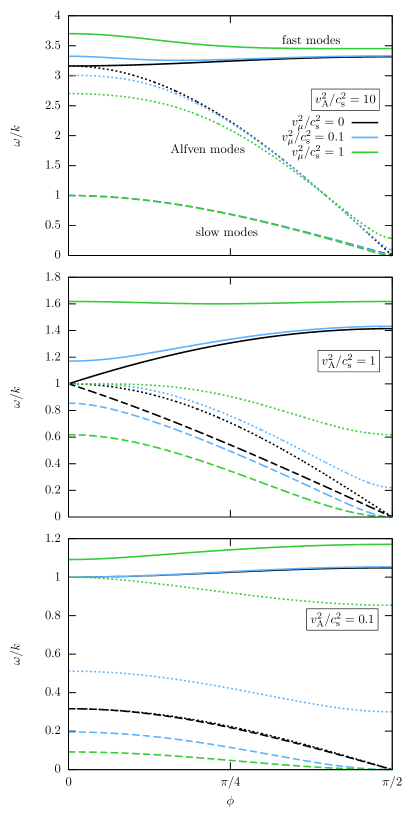
Figure 1.— Influence of the chiral magnetic effect on the MHD waves in a compressible flow. Shown are the ratios $\omega/k$ vs. the angle $\phi$ between the wavevector ${\bm{k}}$ and the equilibrium magnetic field $\bm{B}_{0}$ for the Alfvén wave (dotted lines), the slow magnetosonic wave (dashed lines), and the fast magnetosonic wave (solid lines) for different values of $v_{\mathrm{A}}^{2}/c_{\mathrm{s}}^{2}$ (shown in legends) and different values of $v_{\mu}^{2}/c_{\mathrm{s}}^{2}=$ 0 (black lines), 0.1 (blue lines), and 1 (green lines).

6. Laminar dynamos

First, we study a kinematic problem concerning the evolution of the magnetic field in a given velocity field. In this problem we neglect the back-reaction of the magnetic field on the velocity field. We seek a solution of Equation (45) for perturbations of the following form: $\bm{B}(t,x,z)=B_{y}(t,x,z){\bm{e}}_{y}+\bm{\nabla}\times[A(t,x,z){\bm{e}}_{y}]$, where ${\bm{e}}_{y}$ is the unit vector in the $y$-direction.

6.1. Laminar $v_{\mu}^{2}$ dynamo

We consider the equilibrium configuration: $\mu_{\rm eq}\equiv\mu_{0}=$ const and ${\bm{U}}_{\rm eq}=0$. The functions $B_{y}(t,x,z)$ and $A(t,x,z)$ are determined by the equations

$$\frac{\partial A(t,x,z)}{\partial t} = v_{\mu}\,B_{y}+\eta\Delta A,$$ (62)

$$\frac{\partial B_{y}(t,x,z)}{\partial t} = -v_{\mu}\,\Delta A+\eta\Delta B_{y},$$ (63)

where $v_{\mu}=\eta\,\mu_{0}$, $\Delta=\nabla_{x}^{2}+\nabla_{z}^{2}$, and the remaining components of the magnetic field are given by $B_{x}=-\nabla_{z}A$ and $B_{z}=\nabla_{x}A$. We seek a solution of Equations (62) and (63) of the form $A,B_{y}\propto\exp[\gamma t+i(k_{x}x+k_{z}z)]$. The growth rate of the dynamo instability is given by

$$\gamma=|v_{\mu}\,k|-\eta k^{2},$$ (64)

where $k^{2}=k_{x}^{2}+k_{z}^{2}$. The dynamo instability is excited $(\gamma>0)$ for $k<|\mu_{0}|$. The components of the magnetic field are

$$B_{x}={\rm sgn}\left(\mu_{0}\right)\,{k_{z}\over k}B_{0}\exp(\gamma t)\sin(k_{x}x+k_{z}z),$$ (65)

$$B_{y}=B_{0}\exp(\gamma t)\cos(k_{x}x+k_{z}z),$$ (66)

$$B_{z}=-{\rm sgn}\left(\mu_{0}\right)\,{k_{x}\over k}B_{0}\exp(\gamma t)\sin(k_{x}x+k_{z}z).$$ (67)

The maximum growth rate of the dynamo instability, attained at $k\equiv k^{\rm max}$, is given by

$$\gamma^{\rm max}=v_{\mu}^{2}/4\eta,$$ (68)

where

$$k^{\rm max}=\frac{1}{2}|\mu_{0}|.$$ (69)

6.2. Laminar $v_{\mu}^{2}$–shear dynamo

Here we consider the equilibrium configuration specified by the shear velocity ${\bm{U}}_{\rm eq}=(0,S\,x,0)$, and $\mu_{\rm eq}\equiv\mu_{0}=$ const. This implies that the fluid has a nonzero vorticity ${\bm{W}}=(0,0,S)$ similar to a differential (nonuniform) rotation. The functions $B_{y}(t,x,z)$ and $A(t,x,z)$ are determined by the equations

$$\frac{\partial A(t,x,z)}{\partial t}=v_{\mu}\,B_{y}+\eta\Delta A,$$ (70)

$$\frac{\partial B_{y}(t,x,z)}{\partial t}=-S\nabla_{z}A-v_{\mu}\,\Delta A+\eta\Delta B_{y}.$$ (71)

The first term on the rhs of Equation (71) marks the only difference between the systems of Equations (70) and (71) and Equations (62) and (63). We look for a solution of Equations (70) and (71) of the form $A,B_{y}\propto\exp[\gamma t+i(k_{x}x+k_{z}z-\omega t)]$. The growth rate of the dynamo instability and the frequency of the dynamo waves are

$$\gamma={|v_{\mu}\,k|\over\sqrt{2}}\,\left\{1+\left[1+\left({Sk_{z}\over v_{\mu}\,k^{2}}\right)^{2}\right]^{1\over 2}\right\}^{1\over 2}-\eta k^{2},$$ (72)

$$\omega={\rm sgn}\left(\mu_{0}k_{z}\right)\,{Sk_{z}\over\sqrt{2}k}\,\left\{1+\left[1+\left({Sk_{z}\over v_{\mu}\,k^{2}}\right)^{2}\right]^{1\over 2}\right\}^{-{1\over 2}}.$$

(73)

This solution describes the laminar $v_{\mu}^{2}$–shear dynamo for arbitrary values of the shear rate. Using Equation (72) for $k_{x}=0$, we determine numerically the maximum growth rate of the dynamo instability, $\tilde{\gamma}_{\mathrm{max}}=\gamma_{\mathrm{max}}/|v_{\mu}\,k_{\ast}|$ (attained at $k\equiv k^{\rm max}$) versus the shear rate (see Figure 2). The laminar $v_{\mu}^{2}$–shear dynamo has two limits, one at a low shear rate (corresponding to the $v_{\mu}^{2}$ dynamo; see the dotted lines in Figure 2), and another one at a high shear rate (corresponding to the $v_{\mu}$–shear dynamo, which will be discussed in the next section; see the dashed lines in Figure 2).

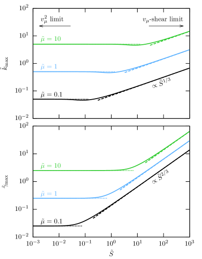
Figure 2.— Maximum nondimensional growth rate $\tilde{\gamma}_{\mathrm{max}}=\gamma_{\mathrm{max}}/|v_{\mu}\,k_{\ast}|$ (bottom panel) and the nondimensional wavenumber $\tilde{k}_{\mathrm{max}}=k_{\mathrm{max}}/k_{\ast}$ (top panel) as a function of the nondimensional shear rate $\tilde{S}=S/|v_{\mu}\,k_{\ast}|$ for different values of $\tilde{\mu}=\mu_{0}/k_{\ast}=$ 0.1 (black), 1 (blue), and 10 (green), where $\gamma_{\mathrm{max}}=\gamma(k=k_{\mathrm{max}})$ and $k_{x}=0$. Here the wavenumber $k_{\ast}$ is based on the characteristic scale of magnetic field variations. The dotted lines at low $S$ indicate the corresponding values for the $v_{\mu}^{2}$ dynamo [see Equations (69) and (68)], while the dashed lines at high $S$ indicate the values for the $v_{\mu}$–shear dynamo [see Equations (80) and (81)].

6.3. Laminar $v_{\mu}$–shear dynamo

In this section we are interested in a situation where the shear term on the rhs of Equation (71) dominates, i.e., where $|S\nabla_{z}A|\gg|v_{\mu}\,\Delta A|$. This condition implies that

$$1<{k\over k_{z}}\ll\frac{S}{v_{\mu}\,k},$$ (74)

i.e., we consider scales with $k\ll S/v_{\mu}$. The growth rate of the dynamo instability and the frequency of the dynamo waves are

$$\gamma=\left({|v_{\mu}\,S\,k_{z}|\over 2}\right)^{1/2}-\eta k^{2},$$ (75)

$$\omega={\rm sgn}\left(\mu_{0}k_{z}\right)\,\left({|v_{\mu}\,S\,k_{z}|\over 2}\right)^{1/2},$$ (76)

and we recall that $k^{2}=k_{x}^{2}+k_{z}^{2}$. The dynamo instability is excited for $k<|v_{\mu}\,S\,k_{z}/2\eta^{2}|^{1/4}$.

The $v_{\mu}$–shear dynamo mechanism acts as follows: the nonuniform stretching of the magnetic field component $B_{x}=-\nabla_{z}A$ by the shear or the differential rotation [see the first term on the right hand side of Equation (71)] causes the generation of a magnetic field in the $y$-direction. But the $v_{\mu}$ effect closes the dynamo loop by generating a magnetic field in the $x$-direction from the $B_{y}$-component [see the first term, $v_{\mu}B_{y}$, on the right side of Equation (70)]. The resulting components of the magnetic field are

$$B_{x} = {\rm sgn}\left(\mu_{0}k_{z}\right)\,\left|{2v_{\mu}\,k_{z}\over S}\right|^{1/2}B_{0}\exp(\gamma t)$$ (77)

$$\times\sin(k_{x}x+k_{z}z-\omega t),$$

$$B_{y} = B_{0}\exp(\gamma t)\cos(k_{x}x+k_{z}z-\omega t),$$ (78)

$$B_{z} = -{\rm sgn}\left(\mu_{0}\right)\,k_{x}\,\left|{2v_{\mu}\over Sk_{z}}\right|^{1/2}B_{0}\exp(\gamma t)$$ (79)

$$\times\sin(k_{x}x+k_{z}z-\omega t).$$

The maximum growth rate of the dynamo instability and the maximum frequency of the dynamo waves, attained at

$$k_{z}^{\rm max}={1\over 4}\left({2|S\,v_{\mu}|\over\eta^{2}}\right)^{1/3},$$ (80)

are given by

$$\gamma^{\rm max} = {3\over 8}\left({S^{2}\,v_{\mu}^{2}\over 2\eta}\right)^{1/3}-\eta k_{x}^{2},$$ (81)

$$\omega^{\rm max} = {{\rm sgn}\left(v_{\mu}\,k_{z}\right)\over 2\eta}\,\left({S^{2}\,v_{\mu}^{2}\over 2\eta}\right)^{1/3}.$$ (82)

7. Turbulent large-scale dynamos

In this section, we study large-scale dynamos in small-scale turbulence with zero mean kinetic helicity. In the presence of small-scale turbulence, large-scale properties of the magnetic field and fluid motion are predicted within the mean-field approach (Moffatt, 1978; Parker, 1979; Krause & Rädler, 1980; Zeldovich et al., 1983), with all quantities decomposed into mean and fluctuations. The fluctuating parts have zero mean value: “overbars” indicate averaging over an ensemble of turbulent velocity fields. We average Equation (50) over the statistics of the random velocity field:

$$\frac{\partial\overline{\mbox{\boldmath$B$}}{}}{\partial t}=\bm{\nabla}\times\left(-{\bm{\overline{\mbox{\boldmath$E$}}{}}}+\overline{\mbox{\boldmath${\cal E}$}}{}+\overline{\mbox{\boldmath${\cal E}$}}{}^{\mu}\right),$$ (83)

where $\overline{\mbox{\boldmath$B$}}{}$ is the mean magnetic field. The total mean electric field, $\overline{\mbox{\boldmath$E$}}{}^{\rm tot}$, has three contributions: $\overline{\mbox{\boldmath$E$}}{}^{\rm tot}=\overline{\mbox{\boldmath$E$}}{}-\overline{\mbox{\boldmath${\cal E}$}}{}-\overline{\mbox{\boldmath${\cal E}$}}{}^{\mu}$. The first contribution is the mean electric field:

$$\overline{\mbox{\boldmath$E$}}{}=-\overline{\bm{U}}\times\overline{\mbox{\boldmath$B$}}{}+\eta\,\bm{\nabla}\times\overline{\mbox{\boldmath$B$}}{}-\overline{v}_{\mu}\,\overline{\mbox{\boldmath$B$}}{},$$ (84)

where $\overline{v}_{\mu}=\eta\,\overline{\mu}$, with $\overline{\mu}$ being the mean chiral chemical potential. Equation (84) is obtained by averaging of Equation (33) for the electric field, $\bm{E}=-\bm{U}\times\bm{B}+\eta\bm{\nabla}\times\bm{B}-v_{\mu}\,\bm{B}$. In Equation (84) we omitted a small term $-\eta\,\overline{\mu^{\prime}\,\bm{b}}$ (which is the second order in $\eta$), where $\bm{b}$ and $\mu^{\prime}$ are magnetic fluctuations and chiral chemical potential fluctuations, respectively. The second, $-\overline{\mbox{\boldmath${\cal E}$}}{}$, and the third, $-\overline{\mbox{\boldmath${\cal E}$}}{}^{\mu}$, contributions to the total mean electric field, $\overline{\mbox{\boldmath$E$}}{}^{\rm tot}$, are related to the mean electromotive force and discussed in the next section.

7.1. Mean electromotive force

The total mean electromotive force is $\mbox{\boldmath$\cal E$}=\overline{\bm{u}\times\bm{b}}=\overline{\mbox{\boldmath${\cal E}$}}{}+\overline{\mbox{\boldmath${\cal E}$}}{}^{\mu}$, where $\bm{u}$ are the fluctuations of the velocity field, $\overline{\mbox{\boldmath${\cal E}$}}{}$ represents the contributions to the mean electromotive force in the absence of the CME, and $\overline{\mbox{\boldmath${\cal E}$}}{}^{\mu}$ are the contributions to the mean electromotive force, caused by the CME. The general form of the mean electromotive force is given by (Rädler, 1980):

$${\cal E}_{i}(\overline{\mbox{\boldmath$B$}}{}) = {\alpha}_{ij}(\overline{\mbox{\boldmath$B$}}{})\overline{B}_{j}-{\eta}_{ij}(\overline{\mbox{\boldmath$B$}}{})(\mbox{\boldmath$\nabla$}{\bf\times}\overline{\mbox{\boldmath$B$}}{})_{j}+({\bf V}_{\rm eff}(\overline{\mbox{\boldmath$B$}}{}){\bf\times}\overline{\mbox{\boldmath$B$}}{})_{i}$$ (85)

$$-[\mbox{\boldmath$\delta$}(\overline{\mbox{\boldmath$B$}}{}){\bf\times}(\mbox{\boldmath$\nabla$}{\bf\times}\overline{\mbox{\boldmath$B$}}{})]_{i}-{\kappa}_{ijk}(\overline{\mbox{\boldmath$B$}}{})({\partial\overline{B}})_{jk}\;,$$

where $({\partial\overline{B}})_{ij}=(\nabla_{i}\overline{B}_{j}+\nabla_{j}\overline{B}_{i})/2$ is the symmetric part of the gradient tensor of the mean magnetic field $\nabla_{i}\overline{B}_{j}$, i.e., $\nabla_{i}\overline{B}_{j}=(\partial\overline{B})_{ij}+\varepsilon_{ijn}(\mbox{\boldmath$\bf\nabla$}{\bf\times}\overline{\mbox{\boldmath$B$}}{})_{n}/2$, the last term on the rhs of this expression is the antisymmetric part of the gradient tensor of the mean magnetic field, and $\varepsilon_{ijk}$ is the fully antisymmetric (Levi-Civita) tensor. Here $\alpha_{ij}(\overline{\mbox{\boldmath$B$}}{})$ and $\eta_{ij}(\overline{\mbox{\boldmath$B$}}{})$ determine the $\alpha$ effect and turbulent magnetic diffusion, respectively: ${\bf V}_{\rm eff}(\overline{\mbox{\boldmath$B$}}{})$ is the effective pumping velocity of the magnetic field: $\kappa_{ijk}(\overline{\mbox{\boldmath$B$}}{})$ describes a contribution to the mean electromotive force related to the symmetric parts of the gradient tensor of the mean magnetic field, $({\partial\overline{B}})_{ij}$, as it appears in anisotropic turbulence; and finally the $\mbox{\boldmath$\delta$}(\overline{\mbox{\boldmath$B$}}{})$ term determines nontrivial behavior of the mean magnetic field in anisotropic turbulence. In Equation (85) we are neglecting terms $\sim\mathcal{O}(\nabla^{2}\overline{B}_{k})$.

The nonlinear transport coefficients defining the mean electromotive force and not related to the CME have been derived in many papers (Rogachevskii & Kleeorin, 2000, 2001; Kleeorin & Rogachevskii, 2003; Rädler et al., 2003; Rogachevskii & Kleeorin, 2004; Rogachevskii et al., 2011). For nonhelical, isotropic, and inhomogeneous turbulence, the mean electromotive force $\overline{\mbox{\boldmath${\cal E}$}}{}$ in the absence of the CME is given by

$$\overline{\mbox{\boldmath${\cal E}$}}{}=-{\eta}_{{}_{T}}\,\mbox{\boldmath$\nabla$}{\bf\times}\overline{\mbox{\boldmath$B$}}{}+{\bf V}_{\rm eff}{\bf\times}\overline{\mbox{\boldmath$B$}}{},$$ (86)

where $\eta_{{}_{T}}=\ell_{0}u_{0}/3$ is the coefficient of turbulent magnetic diffusion and ${\bf V}_{\rm eff}=-(1/2)\mbox{\boldmath$\nabla$}{\eta}_{{}_{T}}$. In this paper we neglect the effect of large-scale shear on the mean electromotive force (Rogachevskii & Kleeorin, 2003, 2004; Kleeorin & Rogachevskii, 2008; Sridhar & Singh, 2014).

To derive equations for the nonlinear coefficients defining the mean electromotive force, we use equations for fluctuations of velocity, ${\bm{u}}$, and magnetic fields, ${\bm{b}}$, and chiral chemical potential, $\mu^{\prime}$:

$${\partial{\bm{u}}\over\partial t} = {1\over\overline{\rho}}\Big{[}-\mbox{\boldmath$\nabla$}p_{\rm tot}+({\bm{b}}\cdot\mbox{\boldmath$\nabla$})\overline{\mbox{\boldmath$B$}}{}+(\overline{\mbox{\boldmath$B$}}{}\cdot\mbox{\boldmath$\nabla$}){\bm{b}}\Big{]}+{\bm{F}}$$ (87)

$$+\nu\Delta{\bm{u}}+{\bm{u}}^{N},$$

$${\partial{\bm{b}}\over\partial t} = (\overline{\mbox{\boldmath$B$}}{}\cdot\mbox{\boldmath$\nabla$}){\bm{u}}-({\bm{u}}\cdot\mbox{\boldmath$\nabla$})\overline{\mbox{\boldmath$B$}}{}+\eta\,\bm{\nabla}\times\Big{[}\overline{\mu}\,{\bm{b}}+\mu^{\prime}\,\overline{\mbox{\boldmath$B$}}{}\Big{]}$$ (88)

$$+\eta\Delta{\bm{b}}+{\bm{b}}^{N},$$

$$\frac{\partial\mu^{\prime}}{\partial t} = -(\bm{u}{\bm{\cdot}}\bm{\nabla})\overline{\mu}+\lambda\,\eta\,\Big{[}\bm{b}{\bm{\cdot}}(\bm{\nabla}\times\overline{\mbox{\boldmath$B$}}{})+\overline{\mbox{\boldmath$B$}}{}{\bm{\cdot}}(\bm{\nabla}\times\bm{b})$$ (89)

$$-\mu^{\prime}\,{\overline{\mbox{\boldmath$B$}}{}}^{\,2}-2\overline{\mu}\,\bm{b}{\bm{\cdot}}\overline{\mbox{\boldmath$B$}}{}\Big{]}+D_{5}\Delta\mu^{\prime}+\mu^{N},$$

where $\overline{\rho}$ is the mean fluid density; $\overline{\rho}\,{\bm{F}}$ is a random external stirring force; ${\bm{u}}^{N}$, ${\bm{b}}^{N}$ and $\mu^{N}$ are the nonlinear terms; $p_{\rm tot}=p^{\prime}+\,(\overline{\mbox{\boldmath$B$}}{}\cdot{\bm{b}})$ are the fluctuations of total pressure; and $p^{\prime}$ are the fluctuations of fluid pressure. The velocity ${\bm{u}}$ satisfies to the continuity equation, $\mbox{\boldmath$\nabla$}\cdot{\bm{u}}=0$, and we consider the case with vanishing mean fluid velocity.

The procedures described in Appendix C yield the contribution to the mean electromotive force caused by the CME for an arbitrary mean magnetic field:

$$\overline{\mbox{\boldmath${\cal E}$}}{}^{\mu}={\bm{\alpha}}^{\mu}(\overline{\mbox{\boldmath$B$}}{})\overline{B}+{\bf V}^{\mu}_{\rm eff}(\overline{\mbox{\boldmath$B$}}{}){\bf\times}\overline{\mbox{\boldmath$B$}}{}.$$ (90)

The chiral tensor ${\bm{\alpha}}^{\mu}(\overline{\mbox{\boldmath$B$}}{})\equiv{\alpha}^{\mu}_{ij}(\overline{\mbox{\boldmath$B$}}{})$ and the chiral effective pumping velocity ${\bm{V}}_{\rm eff}^{\mu}(\overline{\mbox{\boldmath$B$}}{})$ are given in the next section.

7.2. The $\alpha_{\mu}$ effect for a uniform chiral chemical potential

In this section we discuss the $\alpha_{\mu}$ effect in homogeneous isotropic incompressible and nonhelical turbulence with a uniform chiral chemical potential.

7.2.1 Physics of the $\alpha_{\mu}$ effect

The mechanism of the $\alpha_{\mu}$ effect is related to an interaction between the tangling magnetic fluctuations and the chiral magnetic fluctuations. To understand the physics of the $\alpha_{\mu}$ effect, we discuss here only terms in the induction equation (88) that contribute to this effect:

$${\partial{\bm{b}}\over\partial t} = (\overline{\mbox{\boldmath$B$}}{}\cdot\mbox{\boldmath$\nabla$}){\bm{u}}+\overline{v}_{\mu}\bm{\nabla}\times{\bm{b}}+...,$$ (91)

where dots denote all other terms in the induction equation (88) that contribute to the turbulent diffusion and the chiral effective pumping velocity (see Appendix C). The first term, $(\overline{\mbox{\boldmath$B$}}{}\cdot\mbox{\boldmath$\nabla$}){\bm{u}}$, on the rhs of Equation (91) describes the production of the tangling magnetic fluctuations caused by the tangling of the mean magnetic field $\overline{\mbox{\boldmath$B$}}{}$ by sheared small-scale velocity fluctuations. The second term, $\overline{v}_{\mu}\bm{\nabla}\times{\bm{b}}$, in Equation (91) describes the production of the chiral magnetic fluctuations caused by the interaction of the fluctuations of the electric current $\bm{\nabla}\times{\bm{b}}$ of the tangling magnetic fluctuations and the mean chiral chemical potential, $\overline{\mu}$.

Using dimensional analysis, we estimate the level of the tangling magnetic fluctuations ${\bm{b}}_{\rm tang}=\tau\,(\overline{\mbox{\boldmath$B$}}{}\cdot\mbox{\boldmath$\nabla$}){\bm{u}}$, and the level of the chiral magnetic fluctuations ${\bm{b}}_{\mu}$:

$${\bm{b}}_{\mu}=\tau\,\overline{v}_{\mu}\bm{\nabla}\times{\bm{b}}_{\rm tang}=\tau^{2}\,\overline{v}_{\mu}\bm{\nabla}\times\,[(\overline{\mbox{\boldmath$B$}}{}\cdot\mbox{\boldmath$\nabla$}){\bm{u}}],$$

(92)

where $\tau$ is the characteristic timescale of the random velocity field to be discussed below. The mean electromotive force, $\overline{\mbox{\boldmath${\cal E}$}}{}^{\mu}\equiv\overline{\bm{u}\times{\bm{b}}_{\mu}}$, caused by the CME is given by

$$\overline{\cal E}_{i}^{\mu}=\left(\tau^{2}\,\overline{v}_{\mu}\,\overline{u_{n}\nabla_{i}\nabla_{j}u_{n}}\,\right)\,\overline{B}_{j}\equiv\alpha_{ij}^{\mu}\,\overline{B}_{j}.$$ (93)

Here we took into account that an additional term in $\overline{\cal E}_{i}^{\mu}$ that is proportional to $\nabla_{p}\overline{B}_{j}$, vanishes in homogeneous and nonhelical turbulence. It follows from Equation (93) that the chiral $\alpha_{ij}^{\mu}$ tensor is

$$\alpha_{ij}^{\mu}=\overline{v}_{\mu}\,\tau^{2}\,\overline{u_{n}\nabla_{i}\nabla_{j}u_{n}}=-\overline{v}_{\mu}\,\int\tau^{2}(k)\,k_{i}k_{j}\,\langle{\bm{u}}^{2}\rangle_{\bm{k}}\,d{\bm{k}},$$

(94)

where $\langle{\bm{u}}^{2}\rangle_{\bm{k}}=\overline{{\bm{u}}^{2}}\,\tilde{E}(k)/4\pi k^{2}$, the spectrum function of a random velocity field is $\tilde{E}(k)=(q-1)k_{0}^{-1}(k/k_{0})^{-q}$, the wavenumber varies in the interval $k_{0}<k<k_{d}$, the exponent of the spectrum $q$ changes in the interval $1<q<3$, the wavenumbers $k_{0}=1/\ell_{0}$ and $k_{d}=1/\ell_{d}$ with $k_{0}\ll k_{d}$, and $\ell_{d}$ is the dissipation scale.

For small magnetic Reynolds numbers $({\rm Re}_{{}_{M}}=u_{0}\ell_{0}/\eta\ll 1)$, the characteristic timescale of the random velocity field, $\tau$, is determined by the magnetic diffusion time: $\tau(k)=1/\eta k^{2}$. Note that small magnetic Reynolds numbers imply that $u_{0}\ell_{0}\ll\eta$. On the other hand, in Equation (33) for the electric field we neglected the terms in the second order in $\eta$ which implies that $\eta\ll c/(4\pi\,|\bm{\nabla}\Theta|)$. Combining these two conditions, we obtain that for small magnetic Reynolds numbers $u_{0}\ell_{0}\ll\eta\ll c/(4\pi\,|\bm{\nabla}\Theta|)$. Substituting the magnetic diffusion timescale into Equation (94) and integrating in ${\bm{k}}$ space, we arrive at the following expression for the $\alpha_{\mu}$ effect for ${\rm Re}_{{}_{M}}\ll 1$:

$$\alpha_{\mu}=-{(q-1)\over 3(q+1)}\,{\rm Re}_{{}_{M}}^{2}\,\overline{v}_{\mu}.$$ (95)

For large magnetic Reynolds numbers $({\rm Re}_{{}_{M}}\gg 1)$, the characteristic time, $\tau$, of the random velocity field is determined by the turbulent time:

$$\tau(k)=2\tau_{0}(k/k_{0})^{1-q}.$$ (96)

For very large fluid Reynolds numbers, ${\rm Re}$, the exponent of the energy spectrum of turbulent velocity field $q=5/3$ (the Kolmogorov spectrum). For magnetic Prandtl numbers, ${\rm Pr}_{{}_{M}}\equiv\nu/\eta\geq 1$, the dissipation wavenumber $k_{d}$ is determined by the Kolmogorov scale, i.e., $k_{d}=k_{0}{\rm Re}^{3/4}$. Substituting the turbulent timescale (96) into Equation (94), and integrating in ${\bm{k}}$, space we obtain the following expression for the $\alpha_{\mu}$ effect for ${\rm Re}_{{}_{M}}\gg 1$ and ${\rm Pr}_{{}_{M}}\geq 1$:

$$\alpha_{\mu}=-{2\over 3}\overline{v}_{\mu}\ln{\rm Re}.$$ (97)

For magnetic Prandtl numbers, ${\rm Pr}_{{}_{M}}<1$, the dissipation wavenumber $k_{d}$ is determined by the resistive scale, i.e., $k_{d}=k_{0}{\rm Re}_{{}_{M}}^{3/4}$. In this case after integration in ${\bm{k}}$ space we get the expression for the $\alpha_{\mu}$ effect for ${\rm Re}_{{}_{M}}\gg 1$ and ${\rm Pr}_{{}_{M}}<1$:

$$\alpha_{\mu}=-{2\over 3}\overline{v}_{\mu}\ln{\rm Re}_{{}_{M}}.$$ (98)

In the next sections we derive equations for the $\alpha_{\mu}$ effect using rigorous approaches.

7.2.2 Quasi-linear approach

We consider a kinematic problem of the evolution of a magnetic field in a given random velocity field. We start with a weakly nonlinear case in which the nonlinear term in the induction equation (88) is much smaller than the magnetic diffusion term. This allows us to use the quasi-linear approach. In the frame of this approach we neglect the nonlinear term in Equation (88) but keep the diffusion term. This implies that the quasi-linear approach is only valid for small magnetic Reynolds numbers.

Next, we apply a multiscale approach. In the frame of this approach we use the fast and slow variables, and this allows us to separate small-scale effects (fluctuations) and large-scale effects (mean fields). We assume that the maximum scale of random motions $\ell_{0}$ is much smaller than the characteristic scales of the spatial variations of the mean fields, i.e., there is a separation of scales. Using Equation (88) written in Fourier space, we derive an equation for the cross-helicity tensor $g_{ij}=\overline{b_{i}(\omega,{\bm{k}})u_{j}(-\omega,-{\bm{k}})}$:

$$g_{ij}=G_{\eta}\,\hat{D}_{il}^{-1}\,\Big{[}i({\bm{k}}{\bf\cdot}\overline{\mbox{\boldmath$B$}}{})\delta_{lm}-\overline{B}_{l,m}\Big{]}f_{mj}+O(\eta^{2}),$$

(99)

where $f_{ij}=\overline{u_{i}(\omega,{\bm{k}})u_{j}(-\omega,-{\bm{k}})}$, the operator $\hat{D}_{ij}^{-1}=\delta_{ij}+\tilde{\phi}\,\varepsilon_{ijm}\,(k_{m}/k)+O(\tilde{\phi}^{2})$ is the inverse of $\hat{D}_{ij}=\delta_{ij}-\tilde{\phi}\,\varepsilon_{ijm}k_{m}$, $\,\delta_{ij}$ is the Kronecker unit tensor, $\,\tilde{\phi}=-ik\,G_{\eta}\,\overline{v}_{\mu}$, $\overline{B}_{i,j}=\nabla_{j}\overline{B}_{i}$, and $G_{\eta}(k,\omega)=(\eta k^{2}+i\omega)^{-1}$. In Equation (99) we neglected terms $\sim O[\overline{B}^{2};(\nabla\overline{\mbox{\boldmath$B$}}{})^{2};\nabla^{2}\overline{\mbox{\boldmath$B$}}{}]$. This method allows us to determine the contribution to the mean electromotive force $\overline{\mbox{\boldmath${\cal E}$}}{}^{\mu}=\varepsilon_{mji}\int g_{ij}^{\mu}(\omega,{\bm{k}})\,d{\bm{k}}\,d\omega$, caused by the CME: $\overline{\mbox{\boldmath${\cal E}$}}{}^{\mu}=\alpha_{\mu}\overline{\mbox{\boldmath$B$}}{}$, where the $\alpha_{\mu}$ effect is

$$\alpha_{\mu}=-{(q-1)\over 3(q+1)}\,{\rm Re}_{{}_{M}}^{2}\,\overline{v}_{\mu}.$$ (100)

Here we took into account that $g_{ij}^{\mu}(\omega,{\bm{k}})=-\overline{v}_{\mu}\,G_{\eta}^{2}k_{i}k_{j}f^{(0)}_{mm}(\omega,{\bm{k}})\overline{B}_{j}$ (see Equation (99)), and the correlation function $f^{(0)}_{ij}$ with the superscript $(0)$ corresponds to the background homogeneous isotropic and nonhelical turbulence with a zero mean magnetic field. The details of the derivation of the expression for the $\alpha_{\mu}$ effect are given in Appendix C.1. Note that Equation (100) derived using the quasi-linear approach coincides with Equation (95) obtained using the dimensional analysis.

7.2.3 The $\tau$ approach

Figure 3.— The $\alpha_{\mu}$ effect as a function of $\beta=\sqrt{8}\,\,\overline{B}/B_{\rm eq}$ with $B_{\rm eq}=\left(\rho\,\overline{{\bm{u}}^{2}}\right)^{1/2}$. Solid lines represent the expression given by Equation (105) normalized by $\overline{v}_{\mu}$, while the dashed lines show the asymptotics at low $\beta$ as given by (106) and at high $\beta$ as given by Equation (104). The black lines correspond to a fluid Reynolds number of $\mathrm{Re}=4.48$, the blue lines to $\mathrm{Re}=10^{2}$, and the green lines to $\mathrm{Re}=10^{4}$.

For large fluid and magnetic Reynolds numbers we use the $\tau$ approach, which allows us to derive an equation for the contributions to the mean electromotive force caused by a uniform chiral chemical potential: $\overline{\mbox{\boldmath${\cal E}$}}{}^{\mu}=\alpha_{\mu}\overline{B}$, where the $\alpha_{\mu}$ effect is determined by the following expression:

$$\alpha_{\mu}={4\over 3}\overline{v}_{\mu}\biggl{[}\ln\biggl{(}{1+2\beta^{2}{\rm Re}^{1/2}\over(1+2\beta^{2}){\rm Re}^{1/2}}\biggr{)}+{1\over\beta^{2}}\biggl{(}{\arctan(\sqrt{2}\beta)\over\sqrt{2}\beta}$$

$$\quad-1\biggr{)}-{1\over\beta^{2}{\rm Re}^{1/2}}\biggl{(}{\arctan(\sqrt{2}\beta{\rm Re}^{1/4})\over\sqrt{2}\beta{\rm Re}^{1/4}}-1\biggr{)}\biggr{]},$$ (101)

where $\beta=\sqrt{8}\,\,\overline{B}/B_{\rm eq}$ and $B_{\rm eq}=(\rho\,\overline{{\bm{u}}^{2}})^{1/2}$ are the values of the mean magnetic field under the condition of equipartition – equal fractions of kinetic and magnetic energies. The details of the derivation of Equation (101) are given in Appendix C.2. When $\beta\ll{\rm Re}^{-1/4}\ll 1$, i.e., for a very weak mean magnetic field, the chiral $\alpha_{\mu}$ effect is given by

$$\alpha_{\mu}=-{2\over 3}\overline{v}_{\mu}\ln{\rm Re}\left[1-{12\beta^{2}{\rm Re}^{1/2}\over 5\ln{\rm Re}}\right].$$ (102)

When ${\rm Re}^{-1/4}\ll\beta\ll 1$, i.e., for a weak mean magnetic field, the chiral $\alpha_{\mu}$ effect is

$$\alpha_{\mu}=-{4\over 3}\overline{v}_{\mu}|\ln(2\beta^{2})|\left[1+{2\over 3|\ln(2\beta^{2})|}\right],$$ (103)

whereas for $\beta\gg 1$, i.e., for a stronger mean magnetic field, the chiral $\alpha_{\mu}$ effect is

$$\alpha_{\mu}=-{2\over\beta^{2}}\overline{v}_{\mu}.$$ (104)

Equations (101)–(104) are derived for magnetic Prandtl numbers ${\rm Pr}_{{}_{M}}\equiv\nu/\eta\geq 1$. In the case of ${\rm Pr}_{{}_{M}}<1$, the fluid Reynolds number, ${\rm Re}$, in these equations should be replaced by the magnetic Reynolds number, ${\rm Re}_{{}_{M}}$. In this case the $\alpha_{\mu}$ effect is determined by the following expression:

$$\alpha_{\mu}={4\over 3}\overline{v}_{\mu}\biggl{[}\ln\biggl{(}{1+2\beta^{2}{\rm Re}_{{}_{M}}^{1/2}\over(1+2\beta^{2}){\rm Re}_{{}_{M}}^{1/2}}\biggr{)}+{1\over\beta^{2}}\biggl{(}{\arctan(\sqrt{2}\beta)\over\sqrt{2}\beta}$$

$$\quad-1\biggr{)}-{1\over\beta^{2}{\rm Re}_{{}_{M}}^{1/2}}\biggl{(}{\arctan(\sqrt{2}\beta{\rm Re}_{{}_{M}}^{1/4})\over\sqrt{2}\beta{\rm Re}_{{}_{M}}^{1/4}}-1\biggr{)}\biggr{]}.$$ (105)

For a very weak mean magnetic field, $\beta\ll{\rm Re}_{{}_{M}}^{-1/4}\ll 1$, the $\alpha_{\mu}$ effect is given by

$$\alpha_{\mu}=-{2\over 3}\overline{v}_{\mu}\ln{\rm Re}_{{}_{M}}\left[1-{12\beta^{2}{\rm Re}_{{}_{M}}^{1/2}\over 5\ln{\rm Re}_{{}_{M}}}\right].$$ (106)

For a weak mean magnetic field, ${\rm Re}_{{}_{M}}^{-1/4}\ll\beta\ll 1$, and for a stronger mean magnetic field, $\beta\gg 1$, the $\alpha_{\mu}$ effect is given by Equations (103) and (104), respectively. The normalized $\alpha_{\mu}$ effect as a function of $\beta$ is presented in Figure 3 for different magnetic Reynolds numbers. As follows from this section, the $\alpha_{\mu}$ effect in a homogeneous turbulence is always negative, and it is opposite to the $\overline{v}_{\mu}$ effect.

7.3. $\alpha_{\mu}$ effect and effective pumping velocity for nonuniform chiral chemical potential

In this section we discuss the $\alpha_{\mu}$ effect and effective pumping velocity in inhomogeneous turbulence with a nonuniform chiral chemical potential. Using Equations (C36), (C37), (C42), and (C43) in Appendix C, we determine contributions to the functions $\alpha_{ij}^{\mu}(\overline{\mbox{\boldmath$B$}}{})$ and ${\bm{V}}_{\rm eff}^{\mu}(\overline{\mbox{\boldmath$B$}}{})$ caused by a nonuniform chiral chemical potential and for arbitrary values of the mean magnetic field:

$$\alpha_{ij}^{\mu}(\overline{\mbox{\boldmath$B$}}{}) = \alpha_{\mu}\delta_{ij}+{\eta_{{}_{T}}\eta\,\tau_{0}\over 36}\,S(\beta)\biggl{[}\left(\nabla_{i}\overline{\mu}\right)\nabla_{j}$$ (107)

$$+\left(\nabla_{j}\overline{\mu}\right)\nabla_{i}\biggr{]}\ln\overline{{\bm{u}}^{2}},$$

$${\bm{V}}_{\rm eff}^{\mu}(\overline{\mbox{\boldmath$B$}}{}) = -{\eta_{{}_{T}}\eta\,\tau_{0}\over 36}\,S(\beta)\left(\mbox{\boldmath$\nabla$}\overline{\mu}\right)\times\left(\mbox{\boldmath$\nabla$}\ln\overline{{\bm{u}}^{2}}\right),$$ (108)

where the isotropic part of the $\alpha$ effect is the sum of the contribution (101) for ${\rm Pr}_{{}_{M}}\geq 1$ (or Equation (105) for ${\rm Pr}_{{}_{M}}<1$) and that caused by the combined action of a nonuniform chiral chemical potential and inhomogeneous turbulence:

$$\alpha_{\mu}={\eta_{{}_{T}}\eta\,\tau_{0}\over 18}\,S(\beta)\left(\nabla_{p}\overline{\mu}\right)\left(\nabla_{p}\ln\overline{{\bm{u}}^{2}}\right).$$ (109)

Here the function $S(x)$ is given in Equation (C37) of Appendix C. Below, we give expressions for ${\alpha}_{ij}^{\mu}(\overline{\mbox{\boldmath$B$}}{})$ and ${\bm{V}}_{\rm eff}^{\mu}(\overline{\mbox{\boldmath$B$}}{})$, for weak and strong mean magnetic fields. For a weak field, $\overline{B}\ll\overline{B}_{\rm eq}/3$ (i.e., for $\beta\ll 1$), the functions ${\alpha}_{ij}^{\mu}(\overline{\mbox{\boldmath$B$}}{})$ and ${\bm{V}}_{\rm eff}^{\mu}(\overline{\mbox{\boldmath$B$}}{})$ are given by

$${\alpha}_{ij}^{\mu}(\overline{\mbox{\boldmath$B$}}{}) = {\eta_{{}_{T}}\,\eta\,\tau_{0}\over 6}\,\biggl{(}\left(\nabla_{i}\overline{\mu}\right)\nabla_{j}+\left(\nabla_{j}\overline{\mu}\right)\nabla_{i}\biggr{)}\ln\overline{{\bm{u}}^{2}}$$ (110)

$$+\alpha_{\mu}\delta_{ij},$$

$${\bm{V}}_{\rm eff}^{\mu}(\overline{\mbox{\boldmath$B$}}{}) = -{\eta_{{}_{T}}\,\eta\,\tau_{0}\over 6}\,\left(\mbox{\boldmath$\nabla$}\overline{\mu}\right)\times\left(\mbox{\boldmath$\nabla$}\ln\overline{{\bm{u}}^{2}}\right).$$ (111)

while for a strong field, $\overline{B}\gg\overline{B}_{\rm eq}/3$, the functions ${\alpha}_{ij}^{\mu}(\overline{\mbox{\boldmath$B$}}{})$ and ${\bm{V}}_{\rm eff}^{\mu}(\overline{\mbox{\boldmath$B$}}{})$ are

$${\alpha}_{ij}^{\mu}(\overline{\mbox{\boldmath$B$}}{}) = {\eta_{{}_{T}}\,\eta\,\tau_{0}\,\overline{B}_{\rm eq}\over 22\overline{B}}\,\left[\left(\nabla_{i}\overline{\mu}\right)\nabla_{j}+\left(\nabla_{j}\overline{\mu}\right)\nabla_{i}\right]\ln\overline{{\bm{u}}^{2}}$$ (112)

$$+\alpha_{\mu}\delta_{ij},$$

$${\bm{V}}_{\rm eff}^{\mu}(\overline{\mbox{\boldmath$B$}}{}) = -{\eta_{{}_{T}}\,\eta\,\tau_{0}\,\overline{B}_{\rm eq}\over 22\overline{B}}\left(\mbox{\boldmath$\nabla$}\overline{\mu}\right)\times\left(\mbox{\boldmath$\nabla$}\ln\overline{{\bm{u}}^{2}}\right),$$

The contribution to $\alpha_{\mu}$ caused by the combined action of a nonuniform chiral chemical potential and inhomogeneous turbulence for a weak field is

$$\alpha_{\mu} = {\eta_{{}_{T}}\,\eta\,\tau_{0}\over 3}\,\left(\nabla_{p}\overline{\mu}\right)\nabla_{p}\ln\overline{{\bm{u}}^{2}},$$ (114)

while for a strong field it is

$$\alpha_{\mu} = {\eta_{{}_{T}}\,\eta\,\tau_{0}\,\overline{B}_{\rm eq}\over 11\,\overline{B}}\,\,\left(\nabla_{p}\overline{\mu}\right)\,\nabla_{p}\ln\overline{{\bm{u}}^{2}}.$$ (115)

Note that the chiral transport coefficients, ${\alpha}_{ij}^{\mu}(\overline{\mbox{\boldmath$B$}}{})$ and ${\bm{V}}_{\rm eff}^{\mu}(\overline{\mbox{\boldmath$B$}}{})$, appearing in the expression for the mean electromotive force vanish when $\eta\to 0$.

7.4. Generation of the mean kinetic helicity by the CME

In this section we discuss how the mean kinetic helicity, $\chi_{{}_{K}}=\overline{{\bm{u}}\cdot({\bm{\nabla}}\times{\bm{u}})}$, can be generated by the CME in nonhelical turbulence. Using the Navier-Stokes equation for velocity ${\bm{U}}$ and the equation for vorticity ${\bm{W}}={\bm{\nabla}}\times{\bm{U}}$ we derive the evolution equation for the mean kinetic helicity:

$${\partial\chi_{{}_{K}}\over\partial t} = -2\overline{{\bm{w}}\times({\bm{\nabla}}\times{\bm{b}})}\cdot\overline{\mbox{\boldmath$B$}}{}-2\overline{{\bm{w}}\times{\bm{b}}}\cdot({\bm{\nabla}}\times\overline{\mbox{\boldmath$B$}}{})-\varepsilon_{\chi}$$ (116)

$$-{\bm{\nabla}}\cdot{\bm{F}}_{\chi},$$

where ${\bm{w}}={\bm{\nabla}}\times{\bm{u}}$ are the fluctuations of the vorticity, $\varepsilon_{\chi}\sim\chi_{{}_{K}}/\tau_{0}$ is the rate of the dissipation of the mean kinetic helicity, and ${\bm{F}}_{\chi}$ is the flux of the mean kinetic helicity:

$${\bm{F}}_{\chi} = \overline{{\bm{U}}\times\left[({\bm{\nabla}}\times\bm{B})\times\bm{B}\right]}+\overline{{\bm{W}}\cdot\left(p/\rho+{\bm{U}}/2\right)}$$ (117)

$$-\overline{{\bm{U}}\times\left({\bm{U}}\times{\bm{W}}\right)}.$$

To determine the correlation functions $\overline{{\bm{w}}\times({\bm{\nabla}}\times{\bm{b}})}$ and $\overline{{\bm{w}}\times{\bm{b}}}$, we rewrite these functions in ${\bm{k}}$ space: $\left[\,\overline{{\bm{w}}\times({\bm{\nabla}}\times{\bm{b}})}\,\right]_{\bm{k}}=-\varepsilon_{ijp}k_{n}k_{p}g_{ij}({\bm{k}})$ and $\left[\,\overline{{\bm{w}}\times{\bm{b}}}\,\right]_{\bm{k}}=i(\delta_{ij}k_{n}-\delta_{nj}k_{i})g_{ij}({\bm{k}})$, where $g_{ij}({\bm{k}})=\overline{b_{i}({\bm{k}})u_{j}(-{\bm{k}})}$. To determine the correlation function $g_{ij}({\bm{k}})$ we use the $\tau$ approach (see Appendix C.2). After integration in ${\bm{k}}$ space we obtain the contribution to these correlation functions caused by the CME as

$$\left[\,\overline{{\bm{w}}\times{\bm{b}}}\,\right]_{\mu}=-{\alpha_{\mu}\over 4}(\overline{\mbox{\boldmath$B$}}{}\times{\bm{\nabla}})\overline{{\bm{u}}^{2}},$$ (118)

and $\left[\,\overline{{\bm{w}}\times({\bm{\nabla}}\times{\bm{b}})}\,\right]_{\mu}=0$. This implies that $\left[\,\overline{{\bm{w}}\times{\bm{b}}}\,\right]_{\mu}$ can be nonvanishing only in inhomogeneous turbulence. The generalization of this result to the case of inhomogeneous stratified turbulence, where the density stratification is determined in the anelastic approximation, ${\bm{\nabla}}\cdot(\rho{\bm{b}})=0$, is performed by the replacement ${\bm{\nabla}}\to{\bm{\nabla}}-2{\bm{\lambda}}$, where ${\bm{\lambda}}=-{\bm{\nabla}}\rho/\rho$. Therefore, the evolution of the mean kinetic helicity generated by the CME is determined by the following equation:

$${\partial\chi_{{}_{K}}\over\partial t} = {\alpha_{\mu}\over 2}\left[({\bm{\nabla}}\times\overline{\mbox{\boldmath$B$}}{})\times\overline{\mbox{\boldmath$B$}}{}\right]\cdot{\bm{\nabla}}\ln\left(\rho^{2}\overline{{\bm{u}}^{2}}\right)-\varepsilon_{\chi}$$ (119)

$$-{\bm{\nabla}}\cdot{\bm{F}}_{\chi}.$$

This equation implies that the generation of the mean kinetic helicity by the CME in nonhelical turbulence is a nonlinear effect, i.e., it is quadratic in the mean magnetic field, and it occurs only in inhomogeneous or density-stratified turbulence. The corresponding $\alpha$ effect caused by the generated mean kinetic helicity is much smaller than the $\alpha_{\mu}$ effect considered in Section 7.2.

7.5. Different kinds of turbulent large-scale dynamos

In this section we consider turbulent large-scale dynamos in the presence of uniform and nonuniform chiral chemical potentials. In the case of the nonuniform chiral chemical potential the $\alpha_{\mu}$ effect has additional contributions caused by combined action of the nonuniform chiral chemical potential and a small-scale inhomogeneous turbulence. The mean induction equation is given by

$$\frac{\partial\overline{\mbox{\boldmath$B$}}{}}{\partial t} = \bm{\nabla}\times\biggl{\{}\overline{\bm{U}}\times\overline{\mbox{\boldmath$B$}}{}+\overline{v}_{\mu}\,\overline{\mbox{\boldmath$B$}}{}+{\bm{\alpha}}^{\mu}\overline{\mbox{\boldmath$B$}}{}+{\bf V}^{\mu}_{\rm eff}{\bf\times}\overline{\mbox{\boldmath$B$}}{}$$ (120)

$$-(\eta+\,\eta_{{}_{T}})\bm{\nabla}\times\overline{\mbox{\boldmath$B$}}{}\biggr{\}}.$$

Using this equation, we study different kinds of turbulent large-scale dynamos. We seek a solution of Equation (120) for perturbations of the form $\overline{\mbox{\boldmath$B$}}{}(t,x,z)=\overline{B}_{y}(t,x,z){\bm{e}}_{y}+\bm{\nabla}\times[\overline{A}(t,x,z){\bm{e}}_{y}]$, where ${\bm{e}}_{y}$ is the unit vector directed along the $y$-axis.

7.5.1 Turbulent large-scale $\alpha_{\mu}^{2}$ dynamo

We consider the following equilibrium state: $\overline{\mu}=\overline{\mu}_{\rm eq}=$ const and ${\bm{\overline{\bm{U}}}}_{\rm eq}=0$. The functions $\overline{B}_{y}(t,x,z)$ and $\overline{A}(t,x,z)$ are determined by the following equations:

$$\frac{\partial\overline{A}(t,x,z)}{\partial t}=(\overline{v}_{\mu}+\alpha_{\mu})\,\overline{B}_{y}+(\eta+\,\eta_{{}_{T}})\,\Delta\overline{A},$$ (121)

$$\frac{\partial\overline{B}_{y}(t,x,z)}{\partial t}=-(\overline{v}_{\mu}+\alpha_{\mu})\,\Delta\overline{A}+(\eta+\,\eta_{{}_{T}})\,\Delta\overline{B}_{y},$$ (122)

where $\Delta=\nabla_{x}^{2}+\nabla_{z}^{2}$, and other components of the magnetic field are $\overline{B}_{x}=-\nabla_{z}\overline{A}$ and $\overline{B}_{z}=\nabla_{x}\overline{A}$. Mean-field equations (121) and (122) in the presence of a small-scale turbulence are different from Equations (70) and (71) used in Section 6 for studying the laminar dynamo effects. In particular, these mean-field equations contain two new terms related to (i) the $\alpha_{\mu}$ effect (ii) the turbulent diffusion $\eta_{{}_{T}}$; and (iii) the $v_{\mu}$ effect is replaced in the mean-field equations by the mean $\overline{v}_{\mu}$ effect. We are working under the assumption that the ratio of $\eta_{{}_{T}}/\eta$ related to the magnetic Reynolds number,

$${\rm Re}_{{}_{M}}\equiv\frac{3\eta_{{}_{T}}}{\eta}$$ (123)

is large, i.e., ${\rm Re}_{{}_{M}}\gg 1$. This is the case under for many astrophysical flows, e.g., in the early universe (Banerjee & Jedamzik, 2004, 2003; Jedamzik et al., 1998), in stellar and galactic dynamos (Moffatt, 1978; Parker, 1979; Krause & Rädler, 1980; Zeldovich et al., 1983).

We are looking for a solution of the mean-field equations (121) and (122) in the form

$$\overline{A},\overline{B}_{y}\propto\exp[\gamma t+i(k_{x}x+k_{z}z)].$$

The growth rate of the dynamo instability is given by

$$\gamma=|(\overline{v}_{\mu}+\alpha_{\mu})\,k|-(\eta+\,\eta_{{}_{T}})\,k^{2},$$ (124)

and $k^{2}=k_{x}^{2}+k_{z}^{2}$. The components of the mean magnetic field are

$$\overline{B}_{x} = {\rm sgn}\left(\overline{v}_{\mu}+\alpha_{\mu}\right)\,{k_{z}\over k}\overline{B}_{0}\exp(\gamma t)\sin(k_{x}x+k_{z}z),$$

$$\overline{B}_{y} = \overline{B}_{0}\exp(\gamma t)\cos(k_{x}x+k_{z}z),$$ (126)

$$\overline{B}_{z} = -{\rm sgn}\left(\overline{v}_{\mu}+\alpha_{\mu}\right)\,{k_{x}\over k}\,\overline{B}_{0}\exp(\gamma t)\sin(k_{x}x+k_{z}z).$$

The maximum growth rate of the dynamo instability, attained at $k\equiv k^{\rm max}=|\overline{v}_{\mu}+\alpha_{\mu}|/2(\eta+\,\eta_{{}_{T}})$, is given by

$$\gamma^{\rm max}={(\overline{v}_{\mu}+\alpha_{\mu})^{2}\over 4(\eta+\,\eta_{{}_{T}})}={(\overline{v}_{\mu}+\alpha_{\mu})^{2}\over 4\eta\,(1+\,{\rm Re}_{{}_{M}}/3)}.$$ (128)

For small magnetic Reynolds numbers, this equation yields the correct result for the laminar $v_{\mu}^{2}$ dynamo [see Equation (68)]. For large magnetic Reynolds number, the maximum growth rate of the dynamo instability decreases with ${\rm Re}_{{}_{M}}$, i.e., $\gamma^{\rm max}\propto{\rm Re}_{{}_{M}}^{-1}$.

Since the $\alpha_{\mu}$ effect in a homogeneous turbulence is always negative while the $\overline{v}_{\mu}$ effect is positive, the $\alpha_{\mu}$ effect decreases the $\overline{v}_{\mu}$ effect. Both effects compensate each others at ${\rm Re}_{{}_{M}}=4.48$ (see Figure 3). However, for large fluid and magnetic Reynolds numbers, $\overline{v}_{\mu}\ll|\alpha_{\mu}|$, so we can neglect $\overline{v}_{\mu}$ in the equations of this section. This case corresponds to the turbulent large-scale $\alpha_{\mu}^{2}$ dynamo.

7.5.2 Turbulent large-scale $\alpha_{\mu}^{2}$–shear dynamo

Let us consider an equilibrium with mean velocity shear, $\overline{S}$, i.e., $\overline{\bm{U}}_{\rm eq}=(0,\overline{S}x,0)$, and $\overline{\mu}=\overline{\mu}_{\rm eq}=$ const. The functions $\overline{B}_{y}(t,x,z)$ and $\overline{A}(t,x,z)$ are determined by the following equations:

$$\frac{\partial\overline{A}(t,x,z)}{\partial t} = (\overline{v}_{\mu}+\alpha_{\mu})\,\overline{B}_{y}+(\eta+\,\eta_{{}_{T}})\,\Delta\overline{A},$$ (129)

$$\frac{\partial\overline{B}_{y}(t,x,z)}{\partial t} = -\overline{S}\,\nabla_{z}\overline{A}-(\overline{v}_{\mu}+\alpha_{\mu})\,\Delta\overline{A}$$ (130)

$$+(\eta+\,\eta_{{}_{T}})\,\Delta\overline{B}_{y}.$$

We seek a solution of Equations (129) and (130) of the form

$$\overline{A},\overline{B}_{y}\propto\exp[\gamma t+i(k_{x}x+k_{z}z-\omega t)].$$

The growth rate of the dynamo instability and the frequency of the dynamo waves are given by

$$\gamma={|(\overline{v}_{\mu}+\alpha_{\mu})\,k|\over\sqrt{2}}\,\sqrt{1+\sqrt{1+\left({\overline{S}k_{z}\over(\overline{v}_{\mu}+\alpha_{\mu})\,k^{2}}\right)^{2}}}\\ -(\eta+\,\eta_{{}_{T}})\,k^{2},$$ (131)

$$\omega={\overline{S}k_{z}\over\sqrt{2}k}\,\left\{1+\left[1+\left({\overline{S}k_{z}\over(\overline{v}_{\mu}+\alpha_{\mu})\,k^{2}}\right)^{2}\right]^{1\over 2}\right\}^{-{1\over 2}}\\ \times{\rm sgn}\left[(\overline{v}_{\mu}+\alpha_{\mu})k_{z}\right].$$ (132)

For small magnetic Reynolds numbers, these equations yield the correct results for the laminar $v_{\mu}^{2}$-shear dynamo; see Equations (72) and (73). The dependencies of the maximum dimensionless growth rate $\tilde{\gamma}_{\mathrm{max}}=\gamma_{\mathrm{max}}/|(\overline{v}_{\mu}+\alpha_{\mu})\,k_{\ast}|$ and of the dimensionless wavenumber $\tilde{k}_{\mathrm{max}}=k_{\mathrm{max}}/k_{\ast}$ on the nondimensional shear rate $\tilde{S}=S/|(\overline{v}_{\mu}+\alpha_{\mu})\,k_{\ast}|$ are similar to those shown in Figure 2, after the change $\tilde{\mu}\to(\overline{v}_{\mu}+\alpha_{\mu})/[k\eta(1+{\rm Re}_{{}_{M}}/3)]$.

In the case of very large fluid and magnetic Reynolds numbers, $\overline{v}_{\mu}\ll|\alpha_{\mu}|$, so we can neglect $\overline{v}_{\mu}$ in the equations of this section. This case corresponds to the turbulent large-scale $\alpha_{\mu}^{2}$–shear dynamo for an arbitrary value of the shear.

7.5.3 Turbulent large-scale $\alpha_{\mu}$–shear dynamo

Next, we consider a plasma where the shear term in Equation (130) dominates, i.e., we assume that $k^{2}\,|(\overline{v}_{\mu}+\alpha_{\mu})/k_{z}|\ll|\overline{S}|$. The growth rate of the dynamo instability and the frequency of the dynamo waves are

$$\gamma=\left({|(\overline{v}_{\mu}+\alpha_{\mu})\,\overline{S}\,k_{z}|\over 2}\right)^{1/2}-(\eta+\,\eta_{{}_{T}})\,k^{2},$$

$$\omega={\rm sgn}\left[(\overline{v}_{\mu}+\alpha_{\mu})\,k_{z}\right]\,\left({(\overline{v}_{\mu}+\alpha_{\mu})\,\overline{S}\,k_{z}|\over 2}\right)^{1/2}.$$

(134)

The components of the mean magnetic field are

$$\overline{B}_{x} = {\rm sgn}\left[(\overline{v}_{\mu}+\alpha_{\mu})\,k_{z}\right]\,\left|{2(\overline{v}_{\mu}+\alpha_{\mu})\,k_{z}\over\overline{S}}\right|^{1/2}\overline{B}_{0}\exp(\gamma t)$$ (135)

$$\times\sin(k_{x}x+k_{z}z-\omega t),$$

$$\overline{B}_{y} = \overline{B}_{0}\exp(\gamma t)\cos(k_{x}x+k_{z}z-\omega t),$$ (136)

$$\overline{B}_{z} = -{\rm sgn}\left(\overline{v}_{\mu}+\alpha_{\mu}\right)\,k_{x}\,\left|{2(\overline{v}_{\mu}+\alpha_{\mu})\over\overline{S}k_{z}}\right|^{1/2}\overline{B}_{0}\exp(\gamma t)$$ (137)

$$\times\sin(k_{x}x+k_{z}z-\omega t).$$

The maximum growth rate of the dynamo instability and the maximum frequency of the dynamo waves, attained at $k_{x}=0$ and

$$k_{z}^{\rm max}={1\over 4}\left({2|\overline{S}\,(\overline{v}_{\mu}+\alpha_{\mu})|\over(\eta+\,\eta_{{}_{T}})^{2}}\right)^{1/3},$$ (138)

are given by

$$\gamma^{\rm max} = {3\over 8}\left({\overline{S}^{2}\,(\overline{v}_{\mu}+\alpha_{\mu})^{2}\,\over 2(\eta+\,\eta_{{}_{T}})}\right)^{1/3},$$ (139)

$$\omega^{\rm max} = {{\rm sgn}\left[(\overline{v}_{\mu}+\alpha_{\mu})\,k_{z}\right]\over 2\eta}\left[{\overline{S}^{2}\,(\overline{v}_{\mu}+\alpha_{\mu})^{2}\,\over 2(\eta+\,\eta_{{}_{T}})}\right]^{1/3}.$$

In the case of the nonuniform chiral chemical potential we assumed that the generated $\alpha$ effect due to the combined action of the large-scale shear and inhomogeneous turbulence is smaller than the additional contributions to the $\alpha_{\mu}$ effect caused by the combined action of the nonuniform chiral chemical potential and a small-scale inhomogeneous turbulence. The $\alpha$ effect is estimated by $\alpha=S\ell_{0}^{2}/L_{u}$, where $L_{u}$ is the characteristic scale of the inhomogeneity of the turbulence. The above condition implies that $|\overline{S}|\ll\eta|\bm{\nabla}\overline{\mu}|$. The large-scale shear must satisfy the condition $|\alpha_{\mu}k_{z}|\ll|\overline{S}|$ (see above). These two conditions imply that $k_{z}\ll L_{u}/\ell_{0}^{2}$. If this bound is not satisfied, the contribution to the CME caused by the combined action of the nonuniform chiral chemical potential and a small-scale inhomogeneous turbulence is not important.

7.6. Dynamic nonlinearity in mean-field dynamos

In this section we discuss the dynamic nonlinearity, which can play an important role in nonlinear large-scale magnetic dynamos and in the presence of the CME.

7.6.1 Mean fields

We average Equation (51) over the random velocity field:

$$\frac{\partial\overline{\mbox{\boldmath$A$}}{}}{\partial t}=-{\bm{\overline{\mbox{\boldmath$E$}}{}}}+\overline{\mbox{\boldmath${\cal E}$}}{}+\overline{\mbox{\boldmath${\cal E}$}}{}^{\mu}+\bm{\nabla}\overline{\Phi},$$ (141)

where $\overline{\mbox{\boldmath$B$}}{}=\bm{\nabla}\times\overline{\mbox{\boldmath$A$}}{}$. Multiplying Equation (83) by $\overline{\mbox{\boldmath$A$}}{}$ and Equation (141) by $\overline{\mbox{\boldmath$B$}}{}$, and adding them, we obtain an evolutionary equation for the mean magnetic helicity density, $\overline{\mbox{\boldmath$A$}}{}{\bm{\cdot}}\overline{\mbox{\boldmath$B$}}{}$:

$$\frac{\partial\overline{\mbox{\boldmath$A$}}{}{\bm{\cdot}}\overline{\mbox{\boldmath$B$}}{}}{\partial t}+\bm{\nabla}{\bm{\cdot}}\Big{[}{\bm{\overline{\mbox{\boldmath$E$}}{}}}\times\overline{\mbox{\boldmath$A$}}{}-(\overline{\mbox{\boldmath${\cal E}$}}{}+\overline{\mbox{\boldmath${\cal E}$}}{}^{\mu})\times\overline{\mbox{\boldmath$A$}}{}+\overline{\mbox{\boldmath$B$}}{}\,\overline{\Phi}\Big{]}$$

$$\quad=-2{\bm{\overline{\mbox{\boldmath$E$}}{}}}{\bm{\cdot}}\overline{\mbox{\boldmath$B$}}{}+2(\overline{\mbox{\boldmath${\cal E}$}}{}+\overline{\mbox{\boldmath${\cal E}$}}{}^{\mu}){\bm{\cdot}}\overline{\mbox{\boldmath$B$}}{}.$$ (142)

Averaging Equation (53) over the random velocity field, we find that

$$\frac{\partial(2\overline{\mu}/\lambda)}{\partial t}+\bm{\nabla}{\bm{\cdot}}\big{[}-(2D_{5}/\lambda)\,\bm{\nabla}\overline{\mu}\big{]}=2{\overline{\mbox{\boldmath$E$}}{}}{\bm{\cdot}}{\overline{\mbox{\boldmath$B$}}{}}-2\overline{\mbox{\boldmath${\cal E}$}}{}^{\mu}{\bm{\cdot}}\overline{\mbox{\boldmath$B$}}{}$$

$$\quad+2\eta\,\Big{[}\overline{{\bm{\bm{b}}}\,(\bm{\nabla}\times{\bm{\bm{b}}})}-\overline{\mu}\,\,\overline{{\bm{\bm{b}}}^{2}}\Big{]}.$$ (143)

Adding Equations (142) and (143) we obtain an equation for $\overline{\mbox{\boldmath$A$}}{}{\bm{\cdot}}\overline{\mbox{\boldmath$B$}}{}+2\overline{\mu}/\lambda$, namely,

$$\frac{\partial}{\partial t}\Big{(}\overline{\mbox{\boldmath$A$}}{}{\bm{\cdot}}\overline{\mbox{\boldmath$B$}}{}+2\overline{\mu}/\lambda\Big{)}\\ +\bm{\nabla}{\bm{\cdot}}\Big{[}{\bm{\overline{\mbox{\boldmath$E$}}{}}}\times\overline{\mbox{\boldmath$A$}}{}-(\overline{\mbox{\boldmath${\cal E}$}}{}+\overline{\mbox{\boldmath${\cal E}$}}{}^{\mu})\times\overline{\mbox{\boldmath$A$}}{}+\overline{\mbox{\boldmath$B$}}{}\,\overline{\Phi}\quad-(2D_{5}/\lambda)\,\bm{\nabla}\overline{\mu}\Big{]}\\ =2\overline{\mbox{\boldmath${\cal E}$}}{}{\bm{\cdot}}\overline{\mbox{\boldmath$B$}}{}+2\eta\,\Big{[}\overline{\bm{b}\,(\bm{\nabla}\times\bm{b})}-\overline{\mu}\,\,\overline{\bm{b}^{2}}\Big{]}.$$ (144)

Substituting in Equation (54) ${\bm{A}}=\overline{\mbox{\boldmath$A$}}{}+{\bf a}$, $\bm{B}=\overline{\mbox{\boldmath$B$}}{}+\bm{b}$, $\bm{E}=\overline{\mbox{\boldmath$E$}}{}+\bm{E}^{\prime}$, $\mu=\overline{\mu}+\mu^{\prime}$, $\Phi=\overline{\Phi}+\phi^{\prime}$ and averaging the equation so obtained over the random velocity field, we get

$$\frac{\partial}{\partial t}\Big{(}\overline{\mbox{\boldmath$A$}}{}{\bm{\cdot}}\overline{\mbox{\boldmath$B$}}{}+2\overline{\mu}/\lambda+\overline{{\bf a}{\bm{\cdot}}\bm{b}}\Big{)}+\bm{\nabla}{\bm{\cdot}}\Big{[}{\bm{\overline{\mbox{\boldmath$E$}}{}}}\times\overline{\mbox{\boldmath$A$}}{}-(\overline{\mbox{\boldmath${\cal E}$}}{}+\overline{\mbox{\boldmath${\cal E}$}}{}^{\mu})\times\overline{\mbox{\boldmath$A$}}{}$$

$$\quad+\overline{\mbox{\boldmath$B$}}{}\,\overline{\Phi}-(2D_{5}/\lambda)\,\bm{\nabla}\overline{\mu}+\overline{\bm{E}^{\prime}\times{\bf a}}+\overline{\bm{b}\phi^{\prime}}\Big{]}=0.$$ (145)

7.6.2 Equation for fluctuations of magnetic helicity density

Subtracting Equation (144) from Equation (145), we obtain an evolution equation for the small-scale magnetic helicity density, $\chi_{m}=\overline{{\bf a}{\bm{\cdot}}\bm{b}}$, namely,

$$\frac{\partial\chi_{m}}{\partial t}+\bm{\nabla}{\bm{\cdot}}\Big{[}\overline{\bm{E}^{\prime}\times{\bf a}}+\overline{\bm{b}\phi^{\prime}}\Big{]}\\ =-2\overline{\mbox{\boldmath${\cal E}$}}{}{\bm{\cdot}}\overline{\mbox{\boldmath$B$}}{}-2\eta\,\Big{[}\overline{\bm{b}\,(\bm{\nabla}\times\bm{b})}\quad-\overline{\mu}\,\,\overline{\bm{b}^{2}}\Big{]}.$$ (146)

This equation, taking into account the CME, plays a crucial role in the nonlinear stage of the large-scale (mean-field) dynamo evolution. Without the CME, it has been derived and used for the investigation of the nonlinear evolution of the mean magnetic field in a number of studies (Kleeorin & Ruzmaikin, 1982; Kleeorin et al., 1995; Gruzinov & Diamond, 1994; Kleeorin & Rogachevskii, 1999; Kleeorin et al., 2000; Blackman & Field, 2000; Blackman & Brandenburg, 2002; Brandenburg & Subramanian, 2005). The magnetic fluctuations, $\overline{\bm{b}^{2}}$, are determined in Rogachevskii & Kleeorin (2007). Equation (146) can be used in mean-field simulations of the nonlinear large-scale magnetic dynamos in the presence of the CME.

8. Chiral MHD equations in an expanding universe

In this section we demonstrate that basic properties of the chiral MHD equations, analyzed in this paper, also hold in an expanding universe. There are many excellent reviews where the subject of ordinary MHD in an expanding universe is discussed (see, e.g. Barrow et al., 2007; Subramanian, 2010, 2016; Durrer & Neronov, 2013). Therefore, we will discuss here only the novelties, brought by the presence of the axial current and axial anomaly.

8.1. Axial anomaly in an expanding universe

The axial anomaly in a curved background with metric $g_{\mu\nu}$ has the form

$$\frac{\partial}{\partial x^{\mu}}\Bigl{(}\sqrt{-g}j_{5}^{\mu}\Bigr{)}=\frac{\alpha_{\rm em}}{4\pi\hbar}\bar{\epsilon}^{\mu\nu\lambda\rho}F_{\mu\nu}F_{\lambda\rho},$$ (147)

where $g=\mbox{det}(g_{\mu\nu})$ and $\bar{\epsilon}^{\mu\nu\lambda\rho}$ is a flat-space antisymmetric tensor (e.g., $\bar{\epsilon}^{0123}=+1$). The expanding universe is described by the metric

$$ds^{2}=-c^{2}dt^{2}+a^{2}(t)d\bm{x}^{2}$$ (148)

with $\sqrt{-g}=a^{3}(t)$. As discussed in detail by Subramanian (2010, 2016), an observer measures physical quantities in a local inertial frame. This implies that for the current density $\bm{J}$, for example, the corresponding 4-vector is $j^{\mu}=(\varrho,J^{i}/a)$.

In order to recast Equation (147) in a form similar to that in flat space, we define electric and magnetic fields in terms of the components of the field strength tensor $F_{\mu\nu}$ (see Brandenburg et al., 1996; Subramanian, 2010, for details):

$$F_{0i}=a\,\bm{E}^{i},\quad F_{ij}=a^{2}\,\epsilon_{ijk}\bm{B}^{k}\;,$$ (149)

and write

$$\bar{\epsilon}^{\mu\nu\lambda\rho}F_{\mu\nu}F_{\lambda\rho}=8a^{3}(t)\bm{E}\cdot\bm{B}.$$ (150)

Hence, Equation (147) becomes

$$\frac{1}{a^{3}}\frac{\partial\bigl{(}a^{3}n_{5})}{\partial t}+\bm{\nabla}\cdot(\bm{J}_{5}/a)=\frac{2\alpha_{\rm em}}{\pi\hbar}\bm{E}\cdot\bm{B}.$$ (151)

where $j_{5}^{\mu}=(cn_{5},\bm{J}_{5}/a)$. By introducing comoving quantities (Brandenburg et al., 1996; Banerjee & Jedamzik, 2004; Subramanian, 2010):

$$\tilde{\bm{E}} \equiv a^{2}\bm{E}$$ (152)

$$\tilde{\bm{B}} \equiv a^{2}\bm{B}$$

$$\tilde{n}_{5} \equiv a^{3}n_{5}$$

$$\tilde{\bm{J}}_{5} \equiv{a^{3}}\bm{J}_{5}$$

and switching to the conformal time, $\tilde{t}$,

$$d\tilde{t}\equiv\frac{dt}{a(t)},$$ (153)

we obtain

$$\frac{\partial\tilde{n}_{5}}{\partial\tilde{t}}+\bm{\nabla}\cdot\tilde{\bm{J}}_{5}=\frac{2\alpha_{\rm em}}{\pi\hbar}\tilde{\bm{E}}\cdot\tilde{\bm{B}}$$ (154)

an expression identical to Eq. (3).

The quantity $n_{5}$ is related to $\mu_{5}$ as $n_{5}=\mu_{5}(k_{B}T)^{2}/(6\hbar^{3}c^{3})$, where the temperature $T$ now depends on time. Therefore, if one introduces

$$\tilde{\mu}_{5}\equiv a\mu_{5},$$ (155)

the relation between $\tilde{n}_{5}$ and $\tilde{\mu}_{5}$ is given by

$$\tilde{n}_{5}\approx\frac{k_{B}^{2}\bigl{(}a\,T\bigr{)}^{2}}{6\hbar^{3}c^{3}}\tilde{\mu}_{5}.$$ (156)

Finally, introducing a “comoving” axion field,

$$\frac{D\tilde{\Theta}}{D\tilde{t}}\equiv\frac{\partial\tilde{\Theta}}{\partial\tilde{t}}+\tilde{U}\cdot\bm{\nabla}\tilde{\Theta}\equiv\frac{\alpha_{\rm em}}{\pi\hbar}\tilde{\mu}_{5},$$ (157)

and setting $\tilde{\Lambda}$ via

$$\tilde{\Lambda}^{-2}\equiv\frac{12\alpha_{\rm em}}{\pi}\,\frac{\hbar^{2}c^{3}}{k_{B}^{2}(a\,T)^{2}},$$ (158)

we find that the overall property of relativistic MHD (Brandenburg et al., 1996; Banerjee & Jedamzik, 2004; Jedamzik et al., 1998) holds for chiral MHD as well.

9. Conclusions

In this paper we have investigated laminar and turbulent dynamos in chiral MHD. The chiral effect occurs owing to relativistic fermions in a magnetized plasma and plays an important role. It may explain the origin and evolution of magnetic fields in the early universe, and has applications to the theory of neutron stars and quark–gluon plasmas. To study the different dynamo effects, we use the nonlinear system of chiral MHD equations (45)–(48), where we take into account the feedback of the magnetic field onto the chiral chemical potential in the hydrodynamic flow of the plasma. The sum of magnetic helicity and normalized chiral chemical potential is strictly conserved – independent of the magnetic Reynolds number. This determines the main nonlinearity in the system.

We have considered the one-fluid MHD plasma approximation and studied the modifications of MHD waves due to the CME. We have analyzed three kinds of waves in the plasma, namely, Alfvén waves and fast and slow magnetosonic waves. We have demonstrated that the CME decreases the frequency of Alfvén waves for an incompressible fluid, increases the frequencies of Alfvén waves and fast magnetosonic waves for a compressible flow, and decreases the frequency of slow magnetosonic waves.

The CME has been shown to be responsible for new dynamos. The latter originate from a new term in the chiral induction equation (45) which is proportional to $v_{\mu}=\eta\,\mu$, where $\eta$ is the resistive (Ohmic) magnetic diffusion and $\mu$ is the chiral chemical potential. In a plasma without turbulence, there are laminar $v_{\mu}^{2}$ dynamos (discussed previously) and laminar $v_{\mu}$–shear dynamos (or laminar $v_{\mu}^{2}$–shear dynamos) in sheared fluid flows. In the $v_{\mu}^{2}$ dynamo, all components of the magnetic field are generated by the $v_{\mu}$ effect. In the $v_{\mu}$–shear dynamo, the magnetic field component perpendicular to the shear velocity is stretched by the shear velocity. This generates a component of the magnetic field along the shear velocity. The $v_{\mu}$ effect caused by the CME closes the dynamo loop by generating components of the magnetic field perpendicular to the shear velocity.

In turbulent flows with nonzero mean kinetic helicity, the usual $\alpha$ effect is caused by a mean kinetic helicity, independently of the resistive (Ohmic) magnetic diffusion. In such turbulent flows with large fluid and magnetic Reynolds numbers the CME is not important.

However, in turbulent flows with zero mean kinetic helicity, the CME plays a crucial role and contributes to the mean electromotive force. For large magnetic and fluid Reynolds numbers, a new $\alpha_{\mu}$ effect that is caused by an interaction of the CME and fluctuations of the small-scale current produced by tangling magnetic fluctuations is dominant. The tangling magnetic fluctuations are produced by tangling of the large-scale magnetic field by sheared velocity fluctuations. The $\alpha_{\mu}$ effect causes turbulent $\alpha_{\mu}^{2}$ and $\alpha_{\mu}$–shear (or $\alpha_{\mu}^{2}$–shear) dynamos. In turbulent flows with large magnetic Reynolds numbers, the turbulent magnetic diffusion, $\eta_{{}_{T}}$, is much larger than the resistive (Ohmic) magnetic diffusion $\eta$. This implies that the turbulent magnetic diffusion increases the characteristic scale of the mean magnetic field.

Appendix A Current along the magnetic field: Pedagogical derivation

In this appendix we will explain the origin of the current given by Equation (8) in the simplest setup. It has been first derived by Vilenkin (1980) using the method close to the one sketched here and independently rederived in a number of different ways (Redlich & Wijewardhana, 1985; Tsokos, 1985; Alekseev et al., 1998; Fröhlich & Pedrini, 2000, 2002; Kharzeev et al., 2008; Son & Surowka, 2009; Fukushima et al., 2008). There are many excellent reviews on the subject; see, e.g., Kharzeev et al. (2013). This appendix is intended just to give a basic idea.

Let us consider a uniform magnetic field $\bm{B}=(0,0,B)$. The spectrum of the fermions is given by the following expression; see Section 32 in Berestetsky et al. (1959):

$$E_{\bm{p}}=\pm\sqrt{p_{z}^{2}c^{2}+\hbar c|e|B(2n+1-2s_{z})}$$ (A1)

where $n=0,1,2\dots$; $s_{z}=\pm\frac{1}{2}$ is the projection of the fermion’s spin on the magnetic field ($z$-axis); $E_{\bm{p}}$ is the particle energy; and $p_{z}$ is the $z$ component of particle momentum. As a result, for $n=0$ (lowest Landau level) and for positive $s_{z}=+\frac{1}{2}$, the motion of particles is that of free one-dimensional massless fermions with $E_{\bm{p}}=\pm c|\bm{p}|$. Thus, the particles with $p_{z}>0$ have positive projection of spin $\bm{s}$ onto momentum $\bm{p}$ (right-chiral particles), and the particles with $p_{z}<0$ have negative projection of the spin onto momentum (left-chiral particles). In vacuum (at zero temperature and zero chemical potential), all the states with $E_{\bm{p}}<0$ are filled (the Dirac sea), whereas all the states with $E_{\bm{p}}>0$ are empty. If an electric field is applied parallel to the magnetic field, one will observe the disappearance of left-chiral particles and the appearance of right-chiral anti-particles (or vice versa, depending on the sign of the electric field), so that the total electric charge is conserved. This is the manifestation of the axial anomaly; see the discussion in, e.g., Volovik (1998).

Now, let us introduce finite temperature and chemical potentials $\mu_{L},\mu_{R}$ and fill both left- and right-chiral branches of the lowest Landau level according to the Fermi-Dirac distribution (see Fig. 4):

$$f_{L}(p)=\frac{1}{\exp\left(\frac{c|p_{z}|-\mu_{L}}{k_{B}T}\right)+1},\quad p_{z}<0\ ,$$

$$f_{R}(p)=\frac{1}{\exp\left(\frac{c|p_{z}|-\mu_{R}}{k_{B}T}\right)+1},\quad p_{z}>0\ ,$$ (A2)

where $T$ is the temperature.

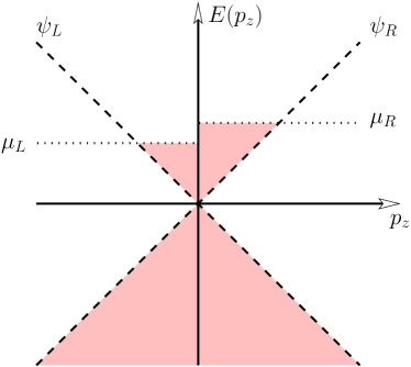
Figure 4.— Lowest Landau level of the massless fermions filled up until the energy $\mu_{L}$ for $p_{z}<0$ and up to the energy $\mu_{R}$ for $p_{z}>0$.

Determining the quantum mechanical expectation value of the electric current $e\langle\psi|\gamma_{z}|\psi\rangle$, and weighting it with the Fermi-Dirac distributions (A3), we find

$$J_{\rm CME} = \frac{eB}{(2\pi\hbar)^{2}}\Big{[}\int\limits^{\infty}_{0}\frac{dp_{z}}{2\pi\hbar}\,\psi_{p_{z}}^{\dagger}\gamma_{z}\psi_{p_{z}}f_{R}(p_{z})$$ (A3)

$$+\int\limits_{-\infty}^{0}\frac{dp_{z}}{2\pi\hbar}\,\psi_{p_{z}}^{\dagger}\gamma_{z}\psi_{p_{z}}f_{L}(p_{z})\Big{]}\ ,$$

where $\psi_{p_{z}}$ are the eigenfunctions of the Dirac equation on the lowest Landau level. Computing Equation (A3), we find that an additional electric current given by Equation (8) appears.

Appendix B Ideal MHD, Lorentz force and Galilean invariance

In this Section we will remind the reader of the derivation of the MHD equations suitable for both relativistic and nonrelativistic case. Most of this material can be found in different textbooks (Landau & Lifshitz, 1959; Melrose, 2012; Weinberg, 1972). We repeat the derivation to demonstrate the origin and structure of the Lorentz force in the case in which the electric current does not have a simple form of the Ohmic current given by Equation (20). We limit ourselves to the case of the ideal MHD, which is sufficient for our purposes.

The equation of ideal (nondissipative) MHD can be derived based on the energy–momentum conservation arguments (see (Landau & Lifshitz, 1959, Section 133-134), (Melrose, 2012, Section 1.4), (Weinberg, 1972, §2.10).

The total energy–momentum tensor $T^{\mu\nu}_{\text{tot}}$ is the sum of the electromagnetic and matter parts: $T^{\mu\nu}_{\text{tot}}\equiv T^{\mu\nu}_{\mathrm{EM}}+T^{\mu\nu}_{\text{mat}}$, where the energy–momentum tensor of the ideal fluid is given by

$$T^{\mu\nu}_{\text{mat}}=(\rho+p/c^{2})u^{\mu}u^{\nu}+p\eta^{\mu\nu},$$ (B1)

where $\rho c^{2}$ is energy density, $p$ is pressure, $\eta_{\mu\nu}$ is the Minkowski metric (whose signature we choose to be $(-,+,+,+)$ and $u^{\mu}$ is the 4-velocity:

$$u^{\mu}\equiv\left(\frac{1}{\sqrt{1-\bm{U}^{2}/c^{2}}},\frac{\bm{U}}{c\sqrt{1-\bm{U}^{2}/c^{2}}}\right)=\gamma\,(1,\bm{U}),$$ (B2)

where the $\gamma$-factor is defined via

$$\gamma=\frac{1}{\sqrt{1-\bm{U}^{2}/c^{2}}}.$$ (B3)

The electromagnetic stress-energy tensor $T^{\mu\nu}_{\mathrm{EM}}$ is

$$T^{\mu\nu}_{\mathrm{EM}}=F_{\mu\lambda}F_{\nu}^{\ \lambda}-\frac{1}{4}\eta_{\mu\nu}F_{\lambda\rho}F^{\lambda\rho}.$$ (B4)

The stress-energy tensor $T^{\mu\nu}_{\mathrm{EM}}$ is evolving as a consequence of the Maxwell equations (17)

$$\frac{\partial T^{\mu\nu}_{\mathrm{EM}}}{\partial x^{\nu}}=-F^{\mu\nu}J_{{\text{tot}},\,\nu}\,,$$ (B5)

where the total current 4-vector $J^{\nu}_{\text{tot}}\equiv(c\rho_{\text{tot}},\bm{J}_{\text{tot}})$. We stress that the rhs of Equation (B5) necessarily contains the total current, which sources the Maxwell equations, independently of its origin.

Taking the divergence of a spatial part ($\mu=i=1,2,3$) of the matter-energy momentum tensor (B1), one finds the relativistic generalization of the Euler equation:

$$\frac{\partial T^{i\nu}_{\text{mat}}}{\partial x^{\nu}}=\gamma^{2}(\rho+p/c^{2})\left[\frac{\partial\bm{U}}{\partial t}+\bm{U}\cdot\bm{\nabla}\bm{U}\right]_{i}+\left(\bm{\nabla}_{i}p+\frac{\bm{U}_{i}}{c^{2}}\frac{\partial p}{\partial t}\right).$$ (B6)

The conservation of the $T^{\mu\nu}_{\text{tot}}$ means that divergence (B6) is equal to $F^{i\nu}J_{{\text{tot}},\,\nu}$, which coincides with the Lorentz force, and

$$\gamma^{2}(\rho+p/c^{2})\left[\frac{\partial\bm{U}}{\partial t}+\bm{U}\cdot\bm{\nabla}\bm{U}\right]=-\bm{\nabla}p-\frac{\bm{U}}{c^{2}}\frac{\partial p}{\partial t}$$

$$\quad+\frac{1}{c}\bm{J}_{\text{tot}}\times\bm{B}+\varrho_{\text{tot}}\bm{E},$$ (B7)

where the last term is zero if the plasma is electrically neutral (i.e. $\varrho_{\text{tot}}=0$). This consideration carries an important assumption: there is no extra energy, associated with $\Theta$ field.

B.1. Galilean invariance

Let us check that Equations (17)–(24) are Galilean invariant. The Galilean transformation acts as follows:

$$\bm{U} \to\bm{U}+\bm{V}_{0},$$ (B8)

$$\bm{B} \to\bm{B}+\frac{\bm{V}_{0}}{c}\times\bm{E},$$

$$\bm{E} \to\bm{E}-\frac{\bm{V}_{0}}{c}\times\bm{B},$$

$$\partial_{t} \to\partial_{t}+\bm{V}_{0}\cdot\bm{\nabla},$$

$$\bm{\nabla} \to\bm{\nabla}.$$

Expression (19) implies that the Ohmic current is given by Equation (20) in a comoving frame, if we consider $\bm{B},\bm{E}$ and $\bm{U}$ in that particular frame. It follows from Equation (19) that there is a $\sigma(\bm{E}\cdot\bm{U})$ contribution to the electric charge density $\varrho_{\text{tot}}$ (again understanding $\bm{E}$ and $\bm{U}$ in a comoving frame).

The curl of $\bm{B}$ in the comoving frame is given by

$$\bm{\nabla}\times\left(\bm{B}+\frac{\bm{V}_{0}}{c}\times\bm{E}\right)=\bm{\nabla}\times\bm{B}+{1\over c}\Big{[}\underbrace{(\bm{\nabla}\cdot\bm{E})}_{=4\pi\varrho_{\rm tot}}\bm{V}_{0}$$

$$\quad-(\bm{V}_{0}\cdot\bm{\nabla})\bm{E}\Big{]}.$$ (B9)

Therefore, the Galilean transformation for $\bm{\nabla}\times\bm{B}$ is:

$$\bm{\nabla}\times\bm{B}\to\bm{\nabla}\times\bm{B}+\frac{4\pi}{c}\varrho_{\text{tot}}\bm{V}_{0}-\frac{1}{c}(\bm{V}_{0}\cdot\bm{\nabla})\bm{E}.$$ (B10)

The last term in Equation (B10), $-(1/c)(\bm{V}_{0}\cdot\bm{\nabla})\bm{E}$, is a part of the displacement current in Equation (17a), which is transformed as $\partial_{t}\bm{E}\to(\partial_{t}+\bm{V}_{0}\cdot\bm{\nabla})\bm{E}$. The second term on the rhs of Equation (B.1) indicates that any current should transform as

$$\bm{J}\to\bm{J}-\varrho_{\text{tot}}\bm{V}_{0}.$$ (B11)

Consider ordinary MHD equations, but keeping $\varrho_{\text{tot}}\neq 0$. Then we have

$$\bm{\nabla}\times\bm{B}=\frac{4\pi}{c}\Bigl{[}\sigma\left(\bm{E}+\frac{\bm{U}\times\bm{B}}{c}\right)-\varrho_{\text{tot}}\bm{U}\Bigr{]},$$ (B12)

and

$$\bm{\nabla}\cdot\bm{E}=4\pi\varrho_{\text{tot}}.$$ (B13)

Expressing $\bm{E}$ from Equation (B12) we find

$$\bm{E}=-\frac{\bm{U}\times\bm{B}}{c}+\sigma^{-1}\left(\frac{c}{4\pi}\bm{\nabla}\times\bm{B}+\varrho_{\text{tot}}\bm{U}\right).$$ (B14)

This expression has correct transformation properties if one takes into account Equation (B10).

Appendix C Procedure of the derivation of the mean electromotive force

We consider an incompressible turbulence with a zero mean kinetic helicity. In order to derive equations for the nonlinear coefficients defining the mean electromotive force, we will use a mean-field approach. Below we consider several methods for the derivation of the equation for the nonlinear mean electromotive force.

C.1. Quasi-linear approach

First, we consider a weakly nonlinear case in which nonlinear terms in Equations (87)–(89) are much smaller than viscous and diffusion terms. This allows us to use the quasi-linear approach. Using this approach, we neglect the nonlinear term in Equation (88) and keep the diffusion term. We also use a multiscale approach, which allows us to separate small-scale effects (fluctuations) from large-scale effects (mean fields). In particular, let us calculate the function $\overline{b_{i}(t,{\bm{x}})\,u_{j}(t,{\bm{x}})}$:

$$\overline{b_{i}(t,{\bm{x}})\,u_{j}(t,{\bm{x}})}=\lim_{t_{1}\to t_{2},{\bm{x}}\to{\bm{y}}}\overline{b_{i}(t_{1},{\bm{x}})\,u_{j}(t_{2},{\bm{y}})}$$

$$=\lim_{\tilde{\tau}\to 0,{\bm{r}}\to 0}\int\,d{\bm{k}}\,\int\,d\omega\,\,\overline{b_{i}(\omega,{\bm{k}})\,u_{j}(-\omega,-{\bm{k}})}$$

$$\times\exp[i{\bm{k}}{\bm{\cdot}}{\bm{r}}+i\omega\,\tilde{\tau}]=\int\,d{\bm{k}}\int\,d\omega\,\,\overline{b_{i}(\omega,{\bm{k}})\,u_{j}(-\omega,-{\bm{k}})},$$

(C1)

where we use new variables, ${\bm{r}}={\bm{x}}-{\bm{y}}$, $\,\tilde{\tau}=t_{1}-t_{2}$, $\,{\bm{k}}=({\bm{k}}_{1}-{\bm{k}}_{2})/2$, $\omega=(\omega_{1}-\omega_{2})/2$, which correspond to small-scale variables, and ${\bm{R}}=({\bm{x}}+{\bm{y}})/2$, $t=(t_{1}+t_{2})/2$, ${\bm{K}}={\bm{k}}_{1}+{\bm{k}}_{2}$, $\Omega=\omega_{1}+\omega_{2}$ which correspond to the large-scale variables. For inhomogeneous turbulence the correlation functions $\langle b_{i}\,u_{j}\rangle$, $\langle u_{i}\,u_{j}\rangle$, etc., depend on the large-scale variable ${\bm{R}}$. We assume also here that there exists a separation of scales, i.e., the maximum scale of random motions $\ell_{0}$ is much smaller than the characteristic scales of inhomogeneities of the mean fields.

Equation (88) written in Fourier space yields

$$\hat{D}_{in}\,b_{n}(\omega,{\bm{k}}) = G_{\eta}\Big{[}i({\bm{k}}{\bf\cdot}\overline{\mbox{\boldmath$B$}}{})\delta_{im}-\overline{B}_{i,m}\Big{]}u_{m}(\omega,{\bm{k}})$$ (C2)

$$+G_{\eta}\,\eta\,\mu^{\prime}\,\bm{\nabla}\times\overline{\mbox{\boldmath$B$}}{},$$

where $\hat{D}_{ij}=\delta_{ij}-\tilde{\phi}\,\varepsilon_{ijm}k_{m}$, $\,\delta_{ij}$ is the Kronecker unit tensor, $\,\tilde{\phi}=-ik\,G_{\eta}\,\overline{v}_{\mu}$, $\overline{B}_{i,j}=\nabla_{j}\overline{B}_{i}$, and $G_{\eta}(k,\omega)=(\eta k^{2}+i\omega)^{-1}$. We consider here the case of a uniform chiral chemical potential, so we neglected terms $\sim O(\nabla\overline{\mu})$ in Equation (C2), where $\mbox{\boldmath$\nabla$}=\partial/\partial{\bm{R}}$. Using Equation (C2) we derive an equation for the cross-helicity tensor $g_{ij}=\overline{b_{i}(\omega,{\bm{k}})u_{j}(-\omega,-{\bm{k}})}$:

$$g_{ij}=G_{\eta}\,\hat{D}_{il}^{-1}\,\Big{[}i({\bm{k}}{\bf\cdot}\overline{\mbox{\boldmath$B$}}{})\delta_{lm}-\overline{B}_{l,m}\Big{]}f_{mj},$$ (C3)

where $f_{ij}=\overline{u_{i}(\omega,{\bm{k}})u_{j}(-\omega,-{\bm{k}})}$ and the operator

$$\hat{D}_{ij}^{-1}=[\delta_{ij}+\tilde{\phi}\,\varepsilon_{ijm}\,(k_{m}/k)+\tilde{\phi}^{2}\,k_{ij}]/(1+\tilde{\phi}^{2})$$ (C4)

is the inverse of $\hat{D}_{ij}$, i.e., $\hat{D}_{in}^{-1}\,\hat{D}_{nj}=\delta_{ij}$. In Equation (C3) we neglected terms $\sim O[\overline{B}^{2};(\nabla\overline{\mbox{\boldmath$B$}}{})^{2};\nabla^{2}\overline{\mbox{\boldmath$B$}}{}]$. The mean electromotive force is defined as $\overline{\mbox{\boldmath${\cal E}$}}{}\equiv\overline{{\bm{u}}\times{\bm{b}}}=\varepsilon_{mji}\int g_{ij}(\omega,{\bm{k}})\,d{\bm{k}}\,d\omega$. The contribution to the mean electromotive force $\overline{\mbox{\boldmath${\cal E}$}}{}^{\mu}$ caused by the chiral effect is obtained using Equation (C3):

$$\overline{\cal E}^{\mu}_{m}=\left(\int a_{ij}^{\mu}(\omega,{\bm{k}})\,d\omega\,d{\bm{k}}\right)\,\overline{B}_{j},$$ (C5)

where

$$a_{ij}^{\mu}(\omega,{\bm{k}})=-\overline{v}_{\mu}\,G_{\eta}^{2}k_{i}k_{j}f^{(0)}_{mm}(\omega,{\bm{k}})+O(\overline{v}_{\mu}^{2}),$$ (C6)

The correlation functions with the superscript $(0)$ correspond to the background turbulence with a zero mean magnetic field. To integrate in $\omega$ and ${\bm{k}}$ space, we use the following model for the background isotropic, homogeneous and nonhelical turbulence:

$$f_{ij}^{(0)}(\omega,{\bm{k}}) = {\tilde{E}(k)\,\tilde{\Phi}(\omega)\over 8\pi\,k^{2}}\Big{[}\delta_{ij}-{k_{i}\,k_{j}\over k^{2}}\Big{]}\overline{{\bm{u}}^{2}},$$ (C7)

where the energy spectrum function $\tilde{E}(k)=(q-1)k_{0}^{-1}(k/k_{0})^{-q}$ with the exponent $1<q<3$ and for $k_{0}<k<k_{d}$. Here $k_{0}=1/\ell_{0}$, $k_{d}$ is the wavenumber based on the dissipation scale, and $k_{0}\ll k_{d}$. We consider the frequency function $\tilde{\Phi}(\omega)$ in the form of the Lorentz profile: $\tilde{\Phi}(\omega)=1/[\pi\,\tau_{c}\,(\omega^{2}+\tau_{c}^{-2})]$, where $\tau_{c}$ is the characteristic correlation time of random velocity field. This model for the frequency function corresponds to the correlation function

$$\langle u_{i}(t)u_{j}(t+\tau)\rangle\propto\exp(-\tau/\tau_{c}).$$ (C8)

After integration in $\omega$ and ${\bm{k}}$ space in Equations (C5), we obtain the contribution to the mean electromotive force $\overline{\mbox{\boldmath${\cal E}$}}{}^{\mu}$ caused by the CME $\overline{\mbox{\boldmath${\cal E}$}}{}^{\mu}=\alpha_{\mu}\overline{\mbox{\boldmath$B$}}{}$, where the $\alpha_{\mu}$ effect is determined by Equation (100).

C.2. The $\tau$ approach

In this section we consider the case of large hydrodynamic and magnetic Reynolds numbers. This implies that the nonlinear terms in Equations (87)–(89) are much larger than viscous and diffusion terms. To exclude the pressure term from the equation of motion (87) we calculate $\mbox{\boldmath$\nabla$}{\bf\times}(\mbox{\boldmath$\nabla$}{\bf\times}{\bm{u}})$. Using Equations (87)–(89) written in Fourier space, we derive equations for the correlation functions of the velocity field $f_{ij}=\overline{u_{i}u_{j}}$, the magnetic field $h_{ij}=\overline{b_{i}b_{j}}$, the cross-helicity $g_{ij}=\overline{b_{i}u_{j}}$, the flux of chemical potential $s_{j}=\overline{\mu^{\prime}u_{j}}$ and the correlation $q_{i}=\overline{\mu^{\prime}b_{i}}$:

$${\partial f_{ij}({\bm{k}})\over\partial t} = i({\bm{k}}{\bf\cdot}\overline{\mbox{\boldmath$B$}}{})\Phi_{ij}+I^{f}_{ij}+F_{ij}+f_{ij}^{N},$$ (C9)

$${\partial h_{ij}({\bm{k}})\over\partial t} = -i({\bm{k}}{\bf\cdot}\overline{\mbox{\boldmath$B$}}{})\Phi_{ij}+I^{h}_{ij}+h_{ij}^{N},$$ (C10)

$${\partial g_{ij}({\bm{k}})\over\partial t} = i({\bm{k}}{\bf\cdot}\overline{\mbox{\boldmath$B$}}{})[f_{ij}({\bm{k}})-h_{ij}({\bm{k}})-h_{ij}^{(H)}]+I^{g}_{ij}$$

$$+i\eta\varepsilon_{inm}k_{n}\left[s_{j}({\bf k})\overline{B}_{m}+g_{mj}({\bm{k}})\overline{\mu}\right]+g_{ij}^{N}\;,$$

$${\partial s_{j}({\bm{k}})\over\partial t} = -i({\bm{k}}{\bf\cdot}\overline{\mbox{\boldmath$B$}}{})q_{j}+I^{s}_{j}+s_{j}^{N}+O(\eta),$$ (C12)

$${\partial q_{i}({\bm{k}})\over\partial t} = -i({\bm{k}}{\bf\cdot}\overline{\mbox{\boldmath$B$}}{})s_{i}+I^{q}_{i}+q_{i}^{N}+O(\eta),$$ (C13)

where hereafter we omitted arguments $t$ and ${\bm{R}}$ in the correlation functions, the mean fluid density is included in the definition of the magnetic field, so that the magnetic field is measured in units of the Alfvén speed, and we neglected terms $\sim O(\nabla^{2})$. Here $\Phi_{ij}({\bm{k}})=g_{ij}({\bm{k}})-g_{ji}(-{\bm{k}}),$ $\,F_{ij}({\bm{k}})=\overline{\tilde{F}_{i}({\bf k})u_{j}(-{\bm{k}})}+\overline{u_{i}({\bm{k}})\tilde{F}_{j}(-{\bm{k}})},$ and ${\bm{\tilde{}}F}({\bm{k}})={\bm{k}}{\bf\times}({\bm{k}}{\bf\times}{\bm{F}}({\bm{k}}))/k^{2}$. The source terms, $I_{ij}^{f},\,I_{ij}^{h},\,I_{ij}^{g},...$, which contain the large-scale spatial derivatives of the mean fields, are given by

$$I_{ij}^{f}={1\over 2}(\overline{\mbox{\boldmath$B$}}{}{\bf\cdot}\mbox{\boldmath$\nabla$})\Phi_{ij}^{(P)}+[g_{qj}({\bm{k}})(2P_{in}(k)-\delta_{in})$$

$$\;+g_{qi}(-{\bm{k}})(2P_{jn}(k)-\delta_{jn})]\overline{B}_{n,q}-\overline{B}_{n,q}k_{n}\Phi_{ijq}^{(P)},$$

$$I_{ij}^{h}={1\over 2}(\overline{\mbox{\boldmath$B$}}{}{\bf\cdot}\mbox{\boldmath$\nabla$})\Phi_{ij}^{(P)}-[g_{iq}({\bm{k}})\delta_{jn}+g_{jq}(-{\bm{k}})\delta_{in}]\overline{B}_{n,q}$$

$$\;-\overline{B}_{n,q}k_{n}\Phi_{ijq}^{(P)},$$

$$I_{ij}^{g}={1\over 2}(\overline{\mbox{\boldmath$B$}}{}{\bf\cdot}\mbox{\boldmath$\nabla$})(f_{ij}+h_{ij})+h_{iq}(2P_{jn}(k)-\delta_{jn})\overline{B}_{n,q}$$

$$\;-f_{nj}\overline{B}_{i,n}-\overline{B}_{n,q}k_{n}(f_{ijq}+h_{ijq})+\eta\varepsilon_{inm}g_{mj}({\bm{k}})\nabla_{n}\overline{\mu},$$

(C18)

$$I_{j}^{s}=-f_{nj}\nabla_{n}\overline{\mu}+O(\eta),$$

$$I_{i}^{q}=-s_{n}\overline{B}_{i,n}-g_{in}(-{\bm{k}})\nabla_{n}\overline{\mu}+O(\eta),$$

where $\Phi_{ij}^{(P)}({\bm{k}})=g_{ij}({\bm{k}})+g_{ji}(-{\bm{k}})$, $P_{ij}(k)=\delta_{ij}-k_{i}\,k_{j}/k^{2}$, the terms $f_{ij}^{N},\,h_{ij}^{N},\,g_{ij}^{N},...$ are determined by the third moments appearing as a result of the nonlinear terms (these terms also include the dissipative viscous and diffusion terms), $f_{ijq}=(1/2)\partial f_{ij}/\partial k_{q},$ and similarly for $h_{ijq}$ and $\Phi_{ijq}^{(P)}$. A stirring force in the Navier-Stokes turbulence is an external parameter, which determines the background turbulence. We have taken into account that in Equation (LABEL:MB7) the terms with symmetric tensors with respect to the indexes “i” and “j” do not contribute to the mean electromotive force because ${\cal E}_{m}=(1/2)\varepsilon_{mji}\,\Phi_{ij}$. In Equations (C.2)–(C18) we have neglected the second and higher derivatives over ${\bf R}$.

In Equations (C10) and (LABEL:MB7) we split the tensor for magnetic fluctuations into nonhelical, $h_{ij},$ and helical, $h_{ij}^{(H)},$ parts. The helical part of the tensor $h_{ij}^{(H)}$ for magnetic fluctuations depends on the magnetic helicity, and it is determined by the dynamic equation that follows from the magnetic helicity conservation arguments (Kleeorin & Ruzmaikin, 1982; Kleeorin et al., 1995; Gruzinov & Diamond, 1994; Kleeorin & Rogachevskii, 1999; Kleeorin et al., 2000; Blackman & Field, 2000; Blackman & Brandenburg, 2002; Brandenburg & Subramanian, 2005). The characteristic time of evolution of the nonhelical part of the magnetic tensor $h_{ij}$ is of the order of the turbulent correlation time $\tau_{0}=\ell_{0}/u_{0}$, while the relaxation time of the helical part of the magnetic tensor $h_{ij}^{(H)}$ is of the order of $\tau_{0}\,{\rm Re}_{{}_{M}}$ (Kleeorin et al., 1995; Kleeorin & Rogachevskii, 1999), where ${\rm Re}_{{}_{M}}=\ell_{0}u_{0}/\eta\gg 1$ is the magnetic Reynolds number and $u_{0}$ is the characteristic turbulent velocity in the maximum scale $\ell_{0}$ of turbulent motions.

The equations for the second moment include the first-order spatial differential operators applied to the third-order moments. A problem arises regarding how to close the system, i.e., how to express the third-order terms $\hat{\cal N}F^{(III)}$ through the lower moments $F^{(II)}$ (Orszag, 1970; Monin & Yaglom, 1975; McComb, 1990). We use the spectral $\tau$ approximation, which postulates that the deviations of the third-moment terms, $\hat{\cal N}F^{(III)}({\bm{k}})$, from the contributions to these terms by the background turbulence, $\hat{\cal N}F^{(III,0)}({\bm{k}})$, can be expressed through similar deviations of the second moments, $F^{(II)}({\bm{k}})-F^{(II,0)}({\bm{k}})$ (Orszag, 1970; Pouquet et al., 1976; Kleeorin et al., 1990, 1996):

$$\hat{\cal N}F^{(III)}({\bm{k}})-\hat{\cal N}F^{(III,0)}({\bm{k}})$$

$$\;\;=-{1\over\tau_{r}(k)}\,\Big{[}F^{(II)}({\bm{k}})-F^{(II,0)}({\bm{k}})\Big{]},$$ (C19)

where $\tau_{r}(k)$ is the scale-dependent relaxation time, which can be identified with the correlation time $\tau(k)$ of the turbulent velocity field for large fluid and magnetic Reynolds numbers. The functions with the superscript $(0)$ correspond to the background turbulence with a zero mean magnetic field. Validation of the $\tau$ approximation for different situations has been performed in numerous numerical simulations and analytical studies (Brandenburg & Subramanian, 2005; Rogachevskii & Kleeorin, 2007; Rogachevskii et al., 2011).

In this study we consider an intermediate nonlinearity that implies that the mean magnetic field is not strong enough in order to affect the correlation time of the turbulent velocity field. The theory for a very strong mean magnetic field can be corrected after taking into account the dependence of the correlation time of the turbulent velocity field on the mean magnetic field.

C.2.1 Solution of second-moment equations

We start with Equations (C9)–(C13) written for nonhelical parts of the tensors. We subtract Equations (C9)–(C13) written for background turbulence (for $\overline{\mbox{\boldmath$B$}}{}=0)$ from those for $\overline{\mbox{\boldmath$B$}}{}\not=0$. Then we use the $\tau$ approximation. Next, we assume that $\eta k^{2}\ll\tau^{-1}(k)$ and $\nu k^{2}\ll\tau^{-1}(k)$ for the inertial range of turbulent flow, and we also assume that the characteristic time of variation of the mean magnetic field $\overline{\mbox{\boldmath$B$}}{}$ is substantially larger than the correlation time $\tau(k)$ for all turbulence scales. Thus, we arrive to the following steady-state solution of the obtained equations:

$$f_{ij}({\bm{k}}) = f_{ij}^{(0)}({\bm{k}})+i\tau({\bm{k}}{\bf\cdot}\overline{\mbox{\boldmath$B$}}{})\Phi_{ij}({\bm{k}})+\tau I_{ij}^{f},$$ (C20)

$$h_{ij}({\bm{k}}) = h_{ij}^{(0)}({\bm{k}})-i\tau({\bm{k}}{\bf\cdot}\overline{\mbox{\boldmath$B$}}{})\Phi_{ij}({\bm{k}})+\tau I_{ij}^{h},$$ (C21)

$$g_{ij}({\bm{k}}) = i\tau({\bm{k}}{\bf\cdot}\overline{\mbox{\boldmath$B$}}{})\left[f_{ij}({\bm{k}})-h_{ij}({\bm{k}})\right]+\tau\Big{\{}I_{ij}^{g}$$ (C22)

$$+i\eta\varepsilon_{inm}k_{n}\left[s_{j}({\bf k})\overline{B}_{m}+g_{mj}({\bm{k}})\overline{\mu}\right]\Big{\}},$$

$$s_{j}({\bm{k}}) = -i\tau({\bm{k}}{\bf\cdot}\overline{\mbox{\boldmath$B$}}{})q_{j}+\tau I_{j}^{s}+O(\eta),$$ (C23)

$$q_{j}({\bm{k}}) = -i\tau({\bm{k}}{\bf\cdot}\overline{\mbox{\boldmath$B$}}{})s_{j}+\tau I^{q}_{j},$$ (C24)

where we have taken into account that $g_{ij}^{(0)}({\bm{k}})=0$. Equations (C20)–(C24) yield

$$\Phi_{ij}=\hat{\Phi}_{ij}+\hat{\Phi}_{ij}^{\mu}+\Phi_{ij}^{(I)},$$ (C25)

$$\hat{\Phi}_{ij}({\bm{k}})={2i\tau({\bm{k}}{\bf\cdot}\overline{\mbox{\boldmath$B$}}{})\over 1+2\Psi}[f_{ij}^{(0)}({\bm{k}})-h_{ij}^{(0)}({\bm{k}})]=2\hat{g}_{ij}({\bm{k}}),$$

(C26)

$$\hat{\Phi}_{ij}^{\mu}=i\eta\tau\left[\varepsilon_{inm}\hat{g}_{mj}({\bm{k}})+\varepsilon_{jnm}\hat{g}_{mi}(-{\bm{k}})\right]\,k_{n}\,\overline{\mu},$$ (C27)

$$\Phi_{ij}^{(I)}({\bf k})={\tau\over 1+2\Psi}\Big{[}\tilde{I}^{g}_{ij}({\bf k})-\tilde{I}^{g}_{ji}(-{\bf k})$$

$$\quad+2i\tau({\bf k}{\bf\cdot}\bar{\bf B})\left(I^{f}_{ij}-I^{h}_{ij}\right)\Big{]},$$ (C28)

where $\Psi({\bm{k}})=2(\tau\,{\bm{k}}{\bf\cdot}\overline{\mbox{\boldmath$B$}}{})^{2}$,

$$\tilde{I}^{g}_{ij}({\bm{k}})=I_{ij}^{g}+i\eta\varepsilon_{inm}k_{n}s_{j}^{(I)}\overline{B}_{m},$$ (C29)

and $\hat{f}_{ij},\hat{h}_{ij},...$ are the solutions of Equations (C20)–(C24) without the source terms $I_{ij}^{f},\,I_{ij}^{h},\,I_{ij}^{g},...$ caused by the gradients of the mean fields, and $f_{ij}^{(I)},h_{ij}^{(I)},g_{ij}^{(I)},...$ are the solutions of these equations caused by the source terms. For example, the function $s_{j}^{(I)}$ entering in Equation (C29) is given by

$$s_{j}^{(I)}({\bf k})={\tau I_{j}^{s}\over 1+\Psi/2}=-{\tau\hat{f}_{nj}\nabla_{n}\overline{\mu}\over 1+\Psi/2}+O(\eta).$$ (C30)

In derivation of Equations (C26)–(C29) we have taken into account the following arguments. Since the solution for the correlation function $\hat{s}_{j}({\bm{k}})$ is proportional to $\eta$, and since we should neglect effects that are quadratic in $\eta$, the correlation function $\hat{s}_{j}({\bm{k}})$ does not contribute to $\hat{\Phi}_{ij}({\bm{k}})$. Using Equations (C20)–(C22) and (C26) we obtain

$$\hat{f}_{ij}({\bm{k}}) \approx {1\over 1+2\Psi}[(1+\Psi)f_{ij}^{(0)}({\bm{k}})+\Psi h_{ij}^{(0)}({\bm{k}})],$$ (C31)

$$\hat{h}_{ij}({\bm{k}}) \approx {1\over 1+2\Psi}[\Psi f_{ij}^{(0)}({\bm{k}})+(1+\Psi)h_{ij}^{(0)}({\bm{k}})].$$ (C32)

Using the derived equations for the second moments $f_{ij},\,h_{ij},g_{ij},...$ we calculate the mean electromotive force ${\cal E}_{l}=\int\tilde{\cal E}_{l}({\bm{k}})\,d{\bm{k}},$ where $\tilde{\cal E}_{l}({\bm{k}})=(1/2)\varepsilon_{lji}\Phi_{ij}({\bm{k}})$. The total mean electromotive force is $\mbox{\boldmath$\cal E$}=\overline{\mbox{\boldmath${\cal E}$}}{}+\overline{\mbox{\boldmath${\cal E}$}}{}^{\mu}$, where $\overline{\mbox{\boldmath${\cal E}$}}{}$ are the contributions to the mean electromotive force without the CME, while $\overline{\mbox{\boldmath${\cal E}$}}{}^{\mu}$ are the contributions to the mean electromotive force caused by the CME. The contribution $\overline{\mbox{\boldmath${\cal E}$}}{}^{\mu}$ is determined using Equations (C28)–(C31):

$$\overline{\cal E}^{\mu}_{l}={1\over 2}\varepsilon_{lji}\int\hat{\Phi}_{ij}^{\mu}({\bm{k}})\,d{\bm{k}}$$

$$\;\;-i\eta\,\varepsilon_{lji}\,\varepsilon_{inm}\,\overline{B}_{m}\int{\tau(k)k_{n}s_{j}^{(I)}({\bm{k}})\over 1+2\Psi}\,d{\bm{k}}.$$ (C33)

The first term in Equations (C33) determines the contribution to $\overline{\mbox{\boldmath${\cal E}$}}{}^{\mu}$ caused by homogeneous turbulence with uniform chiral chemical potential, while the second term in Equation (C33) determines the contribution to $\overline{\mbox{\boldmath${\cal E}$}}{}^{\mu}$ caused by inhomogeneous turbulence with nonuniform chiral chemical potential.

C.2.2 Mean electromotive force in homogeneous nonhelical turbulence

We use the following model for the background isotropic, homogeneous, and nonhelical turbulence:

$$f_{ij}^{(0)}({\bm{k}}) = {\tilde{E}(k)\over 8\pi\,k^{2}}\Big{[}\delta_{ij}-{k_{i}\,k_{j}\over k^{2}}\Big{]}\overline{{\bm{u}}^{2}},$$ (C34)

where the turbulent time $\tau(k)=2\tau_{0}\tilde{\tau}(k)$ with $\,\tilde{\tau}(k)=(k/k_{0})^{-2/3}$, the energy spectrum function $\tilde{E}(k)=-(d\tilde{\tau}(k)/dk)=(2/3)k_{0}^{-1}(k/k_{0})^{-5/3}$ corresponds to the Kolmogorov turbulence, $k_{0}=1/\ell_{0}$ and $\tau_{0}=\ell_{0}/u_{0}$. We also assumed for simplicity that $h_{ij}^{(0)}({\bm{k}})=0$ (i.e., no small-scale dynamo).

After the integration in ${\bm{k}}$ space, we obtain the contributions to the mean electromotive force caused by the uniform chiral chemical potential: $\overline{\mbox{\boldmath${\cal E}$}}{}^{\mu}=\alpha_{\mu}\overline{B}$, where the $\alpha_{\mu}$ effect is determined by Equation (101) for magnetic Prandtl numbers ${\rm Pr}_{{}_{M}}\geq 1$ and by Equation (105) for ${\rm Pr}_{{}_{M}}<1$.

C.2.3 Mean electromotive force in inhomogeneous nonhelical turbulence

Now we use the model for the background isotropic, inhomogeneous, and nonhelical turbulence:

$$f_{ij}^{(0)}({\bm{k}}) = {\tilde{E}(k)\over 8\pi\,k^{2}}\Big{[}\delta_{ij}-{k_{i}\,k_{j}\over k^{2}}+{i\over 2k^{2}}\,\big{(}k_{i}\nabla_{j}-k_{j}\nabla_{i}\big{)}\Big{]}\overline{{\bm{u}}^{2}}.$$

After the integration in ${\bm{k}}$ space, we obtain the contributions to the mean electromotive force caused by the nonuniform chiral chemical potential:

$$\overline{\mbox{\boldmath${\cal E}$}}{}^{\mu}={\eta_{{}_{T}}\eta\,\tau_{0}\over 18}\,S(\beta)\Big{[}\left(\nabla_{i}\overline{\mu}\right)\,\overline{\mbox{\boldmath$B$}}{}{\bm{\cdot}}\bm{\nabla}+\overline{B}_{i}\left(\nabla_{p}\overline{\mu}\right)\nabla_{p}\Big{]}\ln\overline{{\bm{u}}^{2}},$$

(C36)

where

$$S(\beta) = 28A_{1}(\sqrt{2}\beta)-A_{1}(\beta/\sqrt{2})-{9\over\pi}\bar{A}_{1}(2\beta^{2}),$$ (C37)

$$A_{1}(x) = {6\over 7}\biggl{[}{\arctan x\over x}\biggl{(}1+{7\over 9x^{2}}\biggr{)}+{1\over 27}-{7\over 9x^{2}}$$ (C38)

$$-{x^{2}\over 18}\left[1-2x^{2}+2x^{4}\ln(1+x^{-2})\right]\biggr{]},$$

$$\bar{A}_{1}(x) = {2\pi\over x}\biggl{[}(x+1){\arctan(\sqrt{x})\over\sqrt{x}}-1\biggr{]}.$$ (C39)

For $x\ll 1$ these functions are given by

$$A_{1}(x) \sim {2\over 3}\biggl{(}1-{3\over 10}x^{2}\biggr{)},\;\bar{A}_{1}(x)\sim{4\pi\over 3}\biggl{(}1-{1\over 5}x\biggr{)},$$

and for $x\gg 1$ they are given by

$$A_{1}(x) \sim {3\pi\over 7x}-{3\over 2x^{2}}+{\pi\over 3x^{3}},\;\bar{A}_{1}(x)\sim{\pi^{2}\over x^{1/2}}-{4\pi\over x}+{\pi^{2}\over x^{3/2}}.$$

Using these asymptotic formulae, we determine the contributions to the mean electromotive force caused by the nonuniform chiral chemical potential for weak and strong mean magnetic fields. For the weak field, $\beta\ll 1$, the contributions to the mean electromotive force $\overline{\cal E}_{i}^{\mu}$ are given by

$$\overline{\cal E}_{i}^{\mu}={\eta_{{}_{T}}\eta\,\tau_{0}\over 3}\,\left(1-{21\over 20}\beta^{2}\right)\Big{[}\left(\nabla_{i}\overline{\mu}\right)\,\overline{\mbox{\boldmath$B$}}{}{\bm{\cdot}}\bm{\nabla}$$

$$\quad+\overline{B}_{i}\left(\nabla_{p}\overline{\mu}\right)\nabla_{p}\Big{]}\ln\overline{{\bm{u}}^{2}},$$ (C40)

and for strong field $\beta\gg 1$ they are given by

$$\overline{\cal E}_{i}^{\mu}={\eta_{{}_{T}}\eta\,\ell_{0}\over 11\overline{B}}\,\Big{[}\left(\nabla_{i}\overline{\mu}\right)\,\overline{\mbox{\boldmath$B$}}{}{\bm{\cdot}}\bm{\nabla}+\overline{B}_{i}\left(\nabla_{p}\overline{\mu}\right)\nabla_{p}\Big{]}\ln\overline{{\bm{u}}^{2}}.$$

(C41)

We remind here that the mean fluid density is included in the definition of the magnetic field, so that the magnetic field is measured in units of the Alfvén speed, and the electromotive force $\overline{\cal E}_{i}$ is measured in the units of the squared velocity, while $\overline{\mu}$ is measured in the units of the inverse scale.

The total mean electromotive force can be written in the form

$$\overline{\cal E}_{i}=a_{ij}\,\overline{B}_{j}+b_{ijk}\,\overline{B}_{j,k}\;,$$ (C42)

where $\overline{B}_{j,i}=\nabla_{i}\overline{B}_{j}$ and we neglected terms $\sim O(\nabla^{2}\overline{B}_{k})$. The general form of the mean electromotive force is given by Equation (85), where the turbulent transport coefficients are related to the tensors $a_{ij}$ and $b_{ijk}$:

$$\alpha_{ij}(\bar{\bf B})={1\over 2}(a_{ij}+a_{ji}),\;V^{\rm eff}_{k}(\bar{\bf B})={1\over 2}\varepsilon_{kji}\,a_{ij},$$ (C43)

$$\eta_{ij}(\bar{\bf B})={1\over 4}(\varepsilon_{ikp}\,b_{jkp}+\varepsilon_{jkp}\,b_{ikp}),$$ (C44)

$$\delta_{i}={1\over 4}(b_{jji}-b_{jij}),$$ (C45)

$$\kappa_{ijk}(\bar{\bf B})=-{1\over 2}(b_{ijk}+b_{ikj}).$$ (C46)

The separation of terms in Equations (C43) and (C44) is not unique, because a gradient term can always be added to the electromotive force. Using Equations (C36), (C37), (C42), and (C43), we determine the functions $\alpha_{ij}^{\mu}(\overline{\mbox{\boldmath$B$}}{})$ and ${\bm{V}}_{\rm eff}^{\mu}(\overline{\mbox{\boldmath$B$}}{})$ caused by the nonuniform chiral chemical potential, which are given by Equations (107)–(109).

References

- Adler (1969) Adler, S. L. 1969, Phys. Rev., 177, 2426
- Akamatsu & Yamamoto (2013) Akamatsu, Y., & Yamamoto, N. 2013, Phys. Rev. Lett., 111, 052002
- Alekseev et al. (1998) Alekseev, A. Y., Cheianov, V. V., & Fröhlich, J. 1998, Phys. Rev. Lett., 81, 3503
- Artsimovich & Sagdeev (1985) Artsimovich, L. A., & Sagdeev, R. Z. 1985, Plasma Physics for Physicists (Benjamin, New York)
- Banerjee & Jedamzik (2003) Banerjee, R., & Jedamzik, K. 2003, Phys. Rev. Lett., 91, 251301
- Banerjee & Jedamzik (2004) Banerjee, R., & Jedamzik, K. 2004, Phys. Rev., D70, 123003
- Barrow et al. (2007) Barrow, J. D., Maartens, R., & Tsagas, C. G. 2007, Phys. Rept., 449, 131
- Bell (2004) Bell, A. R. 2004, Month. Not. Roy. Astron. Soc., 353, 550
- Bell & Jackiw (1969) Bell, J. S., & Jackiw, R. 1969, Nuovo Cim., A60, 47
- Berestetsky et al. (1959) Berestetsky, V., Lifshitz, E. M., & Pitaevskiy, L. 1959, Quantum Electrodynamics (Pergamon, New York)
- Bieri & Fröhlich (2011) Bieri, S., & Fröhlich, J. 2011, Comptes Rendus Physique, 12, 332
- Biskamp (1997) Biskamp, D. 1997, Nonlinear Magnetohydrodynamics, Cambridge monographs on plasma physics (Cambridge University Press)
- Blackman & Brandenburg (2002) Blackman, E., & Brandenburg, A. 2002, Astrophys. J., 579, 359
- Blackman & Field (2000) Blackman, E. G., & Field, G. 2000, Astrophys. J., 534, 984
- Boyarsky et al. (2012a) Boyarsky, A., Fröhlich, J., & Ruchayskiy, O. 2012a, Phys. Rev. Lett., 108, 031301
- Boyarsky et al. (2015) Boyarsky, A., Fröhlich, J., & Ruchayskiy, O. 2015, Phys. Rev., D92, 043004
- Boyarsky et al. (2012b) Boyarsky, A., Ruchayskiy, O., & Shaposhnikov, M. 2012b, Phys. Rev. Lett., 109, 111602
- Brandenburg et al. (1996) Brandenburg, A., Enqvist, K., & Olesen, P. 1996, Phys. Rev., D54, 1291
- Brandenburg et al. (2017) Brandenburg, A., Schober, J., Rogachevskii, I., Kahniashvili, T., Boyarsky, A., Fröhlich, J., Ruchayskiy, O., & Kleeorin, N. 2017, ApJL, 845, L21
- Brandenburg & Subramanian (2005) Brandenburg, A., & Subramanian, K. 2005, Phys. Rept., 417, 1
- Buividovich & Ulybyshev (2016) Buividovich, P. V., & Ulybyshev, M. V. 2016, Phys. Rev., D94, 025009
- Bykov et al. (2013) Bykov, A. M., Brandenburg, A., Malkov, M. A., & Osipov, S. M. 2013, Space Sci. Rev., 178, 201
- Bykov et al. (2011) Bykov, A. M., Osipov, S. M., & Ellison, D. C. 2011, Month. Not. Roy. Astron. Soc., 410, 39
- Durrer & Neronov (2013) Durrer, R., & Neronov, A. 2013, Astron. Astrophys. Rev., 21, 62
- Dvornikov (2016) Dvornikov, M. 2016, arXiv:1612.06540
- Dvornikov & Semikoz (2012) Dvornikov, M., & Semikoz, V. B. 2012, JCAP, 1202, 040, [Erratum: JCAP1208,E01(2012)]
- Dvornikov & Semikoz (2013) Dvornikov, M., & Semikoz, V. B. 2013, Phys. Rev., D87, 025023
- Dvornikov & Semikoz (2014) Dvornikov, M., & Semikoz, V. B. 2014, JCAP, 1405, 002
- Dvornikov & Semikoz (2015a) Dvornikov, M., & Semikoz, V. B. 2015a, JCAP, 1505, 032
- Dvornikov & Semikoz (2015b) Dvornikov, M., & Semikoz, V. B. 2015b, Phys. Rev., D91, 061301
- Dvornikov & Semikoz (2017) Dvornikov, M., & Semikoz, V. B. 2017, Phys. Rev., D95, 043538
- Fröhlich & Pedrini (2000) Fröhlich, J., & Pedrini, B. 2000, in Mathematical Physics 2000, ed. A. S. Fokas, A. Grigoryan, T. Kibble, & B. Zegarlinski, International Conference on Mathematical Physics 2000, Imperial college (London) (World Scientific Publishing Company)
- Fröhlich & Pedrini (2002) Fröhlich, J., & Pedrini, B. 2002, in Statistical Field Theory, ed. A. Cappelli & G. Mussardo (Kluwer)
- Fukushima et al. (2008) Fukushima, K., Kharzeev, D. E., & Warringa, H. J. 2008, Phys. Rev., D78, 074033
- Giovannini (2013) Giovannini, M. 2013, Phys. Rev., D88, 063536
- Gorbar et al. (2016) Gorbar, E. V., Rudenok, I., Shovkovy, I. A., & Vilchinskii, S. 2016, Phys. Rev., D94, 103528
- Grabowska et al. (2015) Grabowska, D., Kaplan, D. B., & Reddy, S. 2015, Phys. Rev., D91, 085035
- Gruzinov & Diamond (1994) Gruzinov, A. V., & Diamond, P. H. 1994, Physical Review Letters, 72, 1651
- Hirono et al. (2015) Hirono, Y., Kharzeev, D., & Yin, Y. 2015, Phys. Rev., D92, 125031
- Huang & Liao (2013) Huang, X.-G., & Liao, J. 2013, Phys. Rev. Lett., 110, 232302
- Jedamzik et al. (1998) Jedamzik, K., Katalinic, V., & Olinto, A. V. 1998, Phys. Rev., D57, 3264
- Joyce & Shaposhnikov (1997) Joyce, M., & Shaposhnikov, M. E. 1997, Phys. Rev. Lett., 79, 1193
- Kalaydzhyan (2013) Kalaydzhyan, T. 2013, Nucl. Phys., A913, 243
- Kharzeev & Zhitnitsky (2007) Kharzeev, D., & Zhitnitsky, A. 2007, Nucl. Phys., A797, 67
- Kharzeev (2010) Kharzeev, D. E. 2010, Annals Phys., 325, 205
- Kharzeev (2011) Kharzeev, D. E. 2011, J. Phys., G38, 124061
- Kharzeev (2014) Kharzeev, D. E. 2014, Prog. Part. Nucl. Phys., 75, 133
- Kharzeev et al. (2013) Kharzeev, D. E., Landsteiner, K., Schmitt, A., & Yee, H.-U. 2013, Lect. Notes Phys., 871, 1
- Kharzeev et al. (2016) Kharzeev, D. E., Liao, J., Voloshin, S. A., & Wang, G. 2016, Prog. Part. Nucl. Phys., 88, 1
- Kharzeev et al. (2008) Kharzeev, D. E., McLerran, L. D., & Warringa, H. J. 2008, Nucl. Phys., A803, 227
- Kharzeev & Yee (2011a) Kharzeev, D. E., & Yee, H.-U. 2011a, Phys. Rev., D84, 045025
- Kharzeev & Yee (2011b) Kharzeev, D. E., & Yee, H.-U. 2011b, Phys. Rev., D84, 125011
- Kleeorin et al. (1996) Kleeorin, N., Mond, M., & Rogachevskii, I. 1996, Astron. Astrophys., 307, 293
- Kleeorin et al. (2000) Kleeorin, N., Moss, D., Rogachevskii, I., & Sokoloff, D. 2000, Astron. Astrophys., 361, L5
- Kleeorin & Rogachevskii (1999) Kleeorin, N., & Rogachevskii, I. 1999, Phys. Rev. E, 59, 6724
- Kleeorin & Rogachevskii (2003) Kleeorin, N., & Rogachevskii, I. 2003, Phys. Rev. E, 67, 026321
- Kleeorin & Rogachevskii (2008) Kleeorin, N., & Rogachevskii, I. 2008, Phys. Rev. E, 77, 036307
- Kleeorin et al. (1990) Kleeorin, N., Rogachevskii, I., & Ruzmaikin, A. 1990, Zh. Eksp. Teor. Fiz., 97, 1555, [Sov. Phys. JETP 70, 878 (1990)]
- Kleeorin et al. (1995) Kleeorin, N., Rogachevskii, I., & Ruzmaikin, A. 1995, Astron. Astrophys., 297, 159
- Kleeorin & Ruzmaikin (1982) Kleeorin, N., & Ruzmaikin, A. 1982, Magnetohydrodynamics, 2, 17
- Krause & Rädler (1980) Krause, F., & Rädler, K. H. 1980, Mean-Field Magnetohydrodynamics and Dynamo Theory (Pergamon, Oxford)
- Kumar et al. (2016) Kumar, A., Bhatt, J. R., Das, A., & Kaw, P. K. 2016, arXiv:1605.05295
- Kumar et al. (2014) Kumar, A., Bhatt, J. R., & Kaw, P. K. 2014, arXiv:1405.2865
- Kumar et al. (2016) Kumar, A., Bhatt, J. R., & Kaw, P. K. 2016, Physics Letters B, 757, 317
- Landau & Lifshitz (1959) Landau, L. D., & Lifshitz, E. M. 1959, Fluid Mechanics (Pergamon, New York)
- Landsteiner et al. (2013) Landsteiner, K., Megias, E., & Pena-Benitez, F. 2013, Lect. Notes Phys., 871, 433
- Manuel & Torres-Rincon (2015) Manuel, C., & Torres-Rincon, J. M. 2015, Phys. Rev., D92, 074018
- McComb (1990) McComb, W. D. 1990, The Physics of Fluid Turbulence (Clarendon, Oxford)
- Melrose (2012) Melrose, D. 2012, Quantum Plasma Dynamics: Magnetized Plasmas, Lecture Notes in Physics (Springer, New York)
- Miransky & Shovkovy (2015) Miransky, V. A., & Shovkovy, I. A. 2015, Phys. Rept., 576, 1
- Moffatt (1978) Moffatt, H. K. 1978, Magnetic Field Generation in Electrically Conducting Fluids (Cambridge, England, Cambridge University Press)
- Monin & Yaglom (1975) Monin, A. S., & Yaglom, A. M. 1975, Statistical Fluid Mechanics (MIT Press, Cambridge, Massachusetts), Vol. 2.
- Ohnishi & Yamamoto (2014) Ohnishi, A., & Yamamoto, N. 2014, arXiv:1402.4760
- Ooguri & Oshikawa (2012) Ooguri, H., & Oshikawa, M. 2012, Phys. Rev. Lett., 108, 161803
- Orszag (1970) Orszag, S. A. 1970, J. Fluid Mech., 41, 363
- Ozonder (2010) Ozonder, S. 2010, Phys. Rev., C81, 062201
- Parker (1979) Parker, E. 1979, Cosmical Magnetic Fields (Oxford University Press, New York)
- Pavlović et al. (2016) Pavlović, P., Leite, N., & Sigl, G. 2016, JCAP, 1606, 044
- Pavlović et al. (2017) Pavlović, P., Leite, N., & Sigl, G. 2017, Phys. Rev. D , 96, 023504
- Peskin & Schroeder (1995) Peskin, M. E., & Schroeder, D. V. 1995, An Introduction to Quantum Field Theory (Frontiers in Physics) (Westview Press)
- Pouquet et al. (1976) Pouquet, A., Frisch, U., & Leorat, J. 1976, J. Fluid Mech., 77, 321
- Rädler (1980) Rädler, K.-H. 1980, Astron. Nachr., 301, 101
- Rädler et al. (2003) Rädler, K.-H., Kleeorin, N., & Rogachevskii, I. 2003, Geophys. Astrophys. Fluid Dyn., 97, 249
- Redlich & Wijewardhana (1985) Redlich, A. N., & Wijewardhana, L. C. R. 1985, Phys. Rev. Lett., 54, 970
- Rogachevskii & Kleeorin (2000) Rogachevskii, I., & Kleeorin, N. 2000, Phys. Rev. E, 61, 5202
- Rogachevskii & Kleeorin (2001) Rogachevskii, I., & Kleeorin, N. 2001, Phys. Rev. E, 64, 056307
- Rogachevskii & Kleeorin (2003) Rogachevskii, I., & Kleeorin, N. 2003, Phys. Rev. E, 68, 036301
- Rogachevskii & Kleeorin (2004) Rogachevskii, I., & Kleeorin, N. 2004, Phys. Rev. E, 70, 046310
- Rogachevskii & Kleeorin (2007) Rogachevskii, I., & Kleeorin, N. 2007, Phys. Rev. E, 76, 056307
- Rogachevskii et al. (2012) Rogachevskii, I., Kleeorin, N., Brandenburg, A., & Eichler, D. 2012, Astrophys. J., 753, 6
- Rogachevskii et al. (2011) Rogachevskii, I., Kleeorin, N., Kapyla, P., & Brandenburg, A. 2011, Phys. Rev., E84, 056314
- Schlickeiser (2002) Schlickeiser, R. 2002, Cosmic Ray Astrophysics (Springer, Berlin)
- Schober et al. (2017) Schober, J., Rogachevskii, I., Brandenburg, A., Boyarsky, A., Fröhlich, J., Ruchayskiy, O., & Kleeorin, N. 2017, in preparation
- Semikoz et al. (2012) Semikoz, V., Sokoloff, D., & Valle, J. 2012, JCAP, 1206, 008
- Semikoz & Sokoloff (2004) Semikoz, V. B., & Sokoloff, D. D. 2004, A&A, 433, L53
- Semikoz et al. (2009) Semikoz, V. B., Sokoloff, D. D., & Valle, J. W. F. 2009, Phys. Rev., D80, 083510
- Sigl & Leite (2016) Sigl, G., & Leite, N. 2016, JCAP, 1601, 025
- Son & Surowka (2009) Son, D. T., & Surowka, P. 2009, Phys. Rev. Lett., 103, 191601
- Sridhar & Singh (2014) Sridhar, S., & Singh, N. K. 2014, Month. Not. Roy. Astron. Soc., 445, 3770
- Steinberger (1949) Steinberger, J. 1949, Phys. Rev., 76, 1180
- Subramanian (2010) Subramanian, K. 2010, Astron. Nachr., 331, 110
- Subramanian (2016) Subramanian, K. 2016, Reports on Progress in Physics, 79, 076901
- Taghavi & Wiedemann (2015) Taghavi, S. F., & Wiedemann, U. A. 2015, Phys. Rev., C91, 024902
- Tashiro et al. (2012) Tashiro, H., Vachaspati, T., & Vilenkin, A. 2012, Phys. Rev., D86, 105033
- Treiman et al. (1985) Treiman, S., Jackiw, R., Witten, E., & Zumino, B. 1985, Current Algebra and Anomalies, Princeton series in physics (Princeton University Press)
- Tsokos (1985) Tsokos, K. 1985, Phys. Lett., B157, 413
- Vilenkin (1980) Vilenkin, A. 1980, Phys. Rev., D22, 3080
- Volovik (1998) Volovik, G. E. 1998, Physica B Condensed Matter, 255, 86
- Weinberg (1972) Weinberg, S. 1972, Gravitation and Cosmology: principles and applications of general theory of relativity (John Wiley & Sons, Inc)
- Yamamoto (2016) Yamamoto, N. 2016, Phys. Rev., D93, 125016
- Zakharov (2013) Zakharov, V. I. 2013, Lect. Notes Phys., 871, 295
- Zeldovich et al. (1983) Zeldovich, Y. B., Ruzmaikin, A. A., & Sokoloff, D. D. 1983, Magnetic Fields in Astrophysics (Gordon and Breach)
- Zhitnitsky (2012) Zhitnitsky, A. R. 2012, Nucl. Phys., A886, 17
- Zhitnitsky (2013) Zhitnitsky, A. R. 2013, Annals Phys., 336, 462