Chiral magnetohydrodynamics with zero total chirality

Abstract

We study the evolution of magnetic fields coupled with chiral fermion asymmetry in the framework of chiral magnetohydrodynamics with zero initial total chirality. The initial magnetic field has a turbulent spectrum peaking at a certain characteristic scale and is fully helical with positive helicity. The initial chiral chemical potential is spatially uniform and negative. We consider two opposite cases where the ratio of the length scale of the chiral plasma instability (CPI) to the characteristic scale of the turbulence is smaller and larger than unity. These initial conditions might be realized in cosmological models, including certain types of axion inflation. The magnetic field and chiral chemical potential evolve with inverse cascading in such a way that the magnetic helicity and chirality cancel each other at all times, provided there is no spin flipping. The CPI time scale is found to determine mainly the time when the magnetic helicity spectrum attains negative values at high wave numbers. The turnover time of the energy-carrying eddies, on the other hand, determines the time when the peak of the spectrum starts to shift to smaller wave numbers via an inverse cascade. The onset of helicity decay is determined by the time when the chiral magnetic effect becomes efficient at the peak of the initial magnetic energy spectrum, provided the CPI does not grow much. When spin flipping is important, the chiral chemical potential vanishes at late times and the magnetic helicity becomes constant, which leads to a faster increase of the correlation length. This is in agreement with what is expected from magnetic helicity conservation and also happens when the initial total chirality is imbalanced. Our findings have important implications for baryogenesis after axion inflation.

I Introduction

Relativistic plasmas are described by the evolution equations of chiral magnetohydrodynamics (MHD) Son and Surowka (2009); Neiman and Oz (2011); Boyarsky et al. (2012, 2015); Pavlović et al. (2017); Rogachevskii et al. (2017); Brandenburg et al. (2017); Schober et al. (2018); Del Zanna and Bucciantini (2018). Chirality enters in two distinct ways: first, through a nonvanishing chiral chemical potential, $\tilde{\mu}_{5}$, and second, through nonvanishing magnetic helicity density, $\bm{A}\cdot\bm{B}$, where $\bm{B}={\bm{\nabla}}\times\bm{A}$ is the magnetic field expressed in terms of the vector potential $\bm{A}$.

It has been known for some time that fermion chirality can be transferred into magnetic helicity and vice versa through the chiral anomaly Adler (1969); Bell and Jackiw (1969). The transfer of fermion chirality to magnetic helicity occurs through an instability Joyce and Shaposhnikov (1997) known as the chiral plasma instability (CPI) Akamatsu and Yamamoto (2013). This instability is the fastest at a specific wave number, whose value depends on the chiral chemical potential. The transfer from magnetic helicity to chiral chemical potential does not involve any instability, but occurs just through a nonvanishing nonlinear source term in the evolution equation for the chiral chemical potential Boyarsky et al. (2012); Hirono et al. (2015); Schober et al. (2020). These differences in the evolutions of the chiral chemical potential and magnetic field can lead to nontrivial dynamics, which has triggered a lot of research Manuel and Torres-Rincon (2015); Domcke et al. (2019a, 2020). Since fermion chirality is tightly related to the baryon and lepton asymmetries at high temperature in the early Universe, their co-evolution with magnetic helicity in the context of cosmology has also been extensively studied Giovannini and Shaposhnikov (1998a, b); Dvornikov and Semikoz (2012); Tashiro et al. (2012); Long et al. (2014); Fujita and Kamada (2016); Kamada and Long (2016a, b); Pavlović et al. (2017).

Previous investigations mostly assumed an initial imbalance between fermion chirality and magnetic helicity. In many investigations, the initial fermion chirality is nonvanishing while initial magnetic helicity is zero or vice versa. This can lead to a conversion of fermion chirality to a maximally helical magnetic field Boyarsky et al. (2012). Also just spatial fluctuations can lead to magnetic field production Schober et al. (2022a, b). Such chiral asymmetry, which can trigger the CPI, could be generated García-Bellido et al. (1999); Kamada (2018); Domcke et al. (2021) in GUT baryogenesis in the early Universe Yoshimura (1978); Dimopoulos and Susskind (1978); Toussaint et al. (1979); Weinberg (1979); Barr et al. (1979) or weak interactions in compact stars Ohnishi and Yamamoto (2014); Grabowska et al. (2015); Masada et al. (2018); Dvornikov et al. (2020); Matsumoto et al. (2022) (see also Ref. Kamada et al. (2023) and references therein). However, numerical studies on other interesting initial conditions are still lacking, where fermion chirality is exactly opposite to magnetic helicity. Such an initial condition is expected if the chiral symmetry in the fermion sector is only broken through the topological density, $\partial_{\mu}J^{\mu}_{5}=-e^{2}F_{\mu\nu}\tilde{F}^{\mu\nu}/(8\pi^{2}\hbar^{2}c)$, or the chiral anomaly Adler (1969); Bell and Jackiw (1969), with $J_{5}^{\mu}$ being the chiral current and $e^{2}F_{\mu\nu}\tilde{F}^{\mu\nu}/(8\pi^{2}\hbar^{2}c)$ being the topological density. Since the topological density can be written as a total derivative of the magnetic helicity density, the sum of chiral asymmetry and magnetic helicity vanishes when they are generated Domcke and Mukaida (2018).

Configurations with vanishing total chirality are interesting not only in the context of chiral MHD, but also in particle physics and cosmology. At high enough temperatures, realized in the early Universe, the electron Yukawa interaction becomes inefficient for $T\gtrsim 10^{5}\,\mathrm{GeV}$ Campbell et al. (1992); Bödeker and Schröder (2019). There we find the conservation of total chirality because of $\partial_{\mu}J^{\mu}_{e_{R}}=-g_{Y}^{2}Y_{\mu\nu}\tilde{Y}^{\mu\nu}/(16\pi^{2}\hbar^{2}c)$ with $J^{\mu}_{e_{R}}$ being the right-handed electron current and $Y^{\mu\nu}$ being the field strength of the hypercharge gauge field with gauge coupling $g_{Y}$. For instance, in a certain class of axion inflation, configurations with zero net chirality are generated during inflation Domcke and Mukaida (2018), which can be the origin of the observed baryon asymmetry of the Universe Jiménez et al. (2017); Domcke et al. (2019b, 2023) and it could explain the proposed intergalactic magnetic field; see, however, Ref. Kamada and Long (2016b) for the baryon overproduction problem and Ref. Kamada et al. (2021) for the too large baryon isocurvature problem. The main purpose of this paper is to perform a full numerical chiral MHD simulation under the initial condition of vanishing total chirality and provide a better understanding of the nonlinear dynamics in this case.

Before we begin our investigations, it is useful to recall the main findings of earlier work where the total chirality was mostly different from zero. Following the work of Ref. Hirono et al. (2015), who studied a system consisting of the gauge field and the chiral chemical potential, but without fluid velocity fields, and with the initial condition $\langle\bm{A}\cdot\bm{B}\rangle\not=0,\tilde{\mu}_{5}=0$, three stages can be identified: (i) exponential decline of the magnetic helicity together with an increase of $\tilde{\mu}_{5}$, followed by (ii) a continued decrease of the typical peak wave number $k_{\rm p}$, while $\tilde{\mu}_{5}$ stays at its maximum value with $\langle\bm{A}\cdot\bm{B}\rangle$ being essentially zero, and (iii) a phase when all the fermion chirality $\tilde{\mu}_{5}$ gets transferred back to magnetic helicity. As expected, owing to magnetic helicity conservation, and because the magnetic field from the CPI is maximally helical, the magnetic energy density $\langle\bm{B}^{2}\rangle/2$ decays at late times such that $\langle\bm{B}^{2}\rangle\xi_{\rm M}\approx{\rm const}{}$, where $\xi_{\rm M}\equiv k_{\rm p}^{-1}$ is the magnetic correlation length. In other words, both $\langle\bm{B}^{2}\rangle$ and $k_{\rm p}$ decay in the same fashion, but, unlike the expected $t^{-2/3}$ scaling found previously for helical turbulence (Hatori, 1984; Biskamp and Müller, 1999; Kahniashvili et al., 2013; Brandenburg and Kahniashvili, 2017), the authors of Ref. Hirono et al. (2015) find a $t^{-1/2}$ scaling both for $\langle\bm{B}^{2}\rangle$ and $k_{\rm p}$. For sufficiently strong initial magnetic fields, the magnetic Reynolds number can be much larger than unity and the eddy turnover scale much longer than the estimated inverse peak momentum scale, if equipartition between the magnetic field and fluid velocity is established. This suggests that the effect of the fluid velocity cannot be negligible in general.

The earlier analytic study of Ref. Hirono et al. (2015) was revisited using direct numerical simulations of chiral MHD Schober et al. (2020). At large magnetic Reynolds numbers, the authors found clear evidence for a $t^{-2/3}$ scaling of both $\langle\bm{B}^{2}\rangle$ and $k_{\rm p}$ at late times. They also found that the initial evolution is not exponential, as suggested in Ref. Hirono et al. (2015), but linear in time. However, they only considered the case where the initial fermion chirality was zero. When it is finite and balancing exactly the magnetic helicity, the magnetic field decays in a way similar to the case of a strong, nonhelical field Brandenburg et al. (2023), where the decay is governed by the conservation of the Hosking integral Hosking and Schekochihin (2021, 2022); Zhou et al. (2022). This integral describes the strength of magnetic helicity fluctuations on different length scales and has the dimensions of $\,{\rm cm}^{9}\,{\rm s}^{-4}$, which implies the scalings $\xi_{\rm M}\propto t^{4/9}$ and $\langle\bm{B}^{2}\rangle\propto t^{-10/9}$ Hosking and Schekochihin (2021); Zhou et al. (2022); Brandenburg and Larsson (2023). The general validity of the Hosking integral was further demonstrated by applying a corresponding analysis to the decay of a nonhelical magnetic field in neutron star crusts Brandenburg (2023), where the magnetic field evolution is covered by the Hall effect Goldreich and Reisenegger (1992).

Our goal here is to bridge the gap between the two extremes, where the initial chirality is either only in the fermions or only in the magnetic field, and to consider the intermediate case where fermion chirality and magnetic helicity balance to zero, extending the study of the present authors Brandenburg et al. (2023). This is another case where the decay of $\langle\bm{B}^{2}\rangle$ and $k_{\rm p}$ are described by a correspondingly adapted Hosking integral of the total chirality. In the following, we therefore refer to the Hosking integral with the chiral chemical potential included as the “adapted” Hosking integral; see Ref. Brandenburg et al. (2023) for detail.

As mentioned above, our findings on the evolution of the system with vanishing total chirality has significant impact on the present baryon asymmetry of the Universe. Another goal of the present paper is to clarify how the non-trivial co-evolution of the magnetic field and fermion chirality affect the model space of axion inflation consistent with the present Universe, which has not been explored before.

We begin, by presenting the basic equations and the mathematical setup of our simulations in Sect. II. We then discuss the parameter dependence of characteristic time scales, consider the effect of spin flipping, and finally cases where the perfectly vanishing chirality balance is relaxed in Sect. III. Applications to the early Universe are discussed in Sect. IV. Conclusions are presented in Sect. V.

II Chiral magnetohydrodynamics

II.1 Chiral magnetic effect

Using Lorentz-Heaviside units, the Ampère-Maxwell equation for the QED-like model in the MHD limit (omitting the displacement current) reads

$${\bm{\nabla}}\times{\bm{B}}=\frac{1}{c}{\bm{J}}.$$ (1)

The electric current ${\bm{J}}$ is the sum of the Ohmic current and the chiral magnetic effect (CME) Vilenkin (1980); Alekseev et al. (1998); Fukushima et al. (2008),

$${\bm{J}}=\frac{\sigma}{c}\left(c{\bm{E}}+{\bm{u}}\times{\bm{B}}\right)+\frac{e^{2}}{2\pi^{2}\hbar^{2}c}\tilde{\mu}_{5}{\bm{B}},$$ (2)

where $\sigma$ is the electric conductivity (or inverse magnetic diffusivity) and we consider the case with $\tilde{\mu}_{5}\ll(e^{2}/\hbar c)k_{\rm B}T$. By rewriting $c{\bm{E}}=-\partial{\bm{A}}/\partial t$ in the Weyl gauge, $e^{2}/4\pi\hbar c\equiv\alpha$, Eq. (2) is rewritten as

$$\frac{\partial{\bm{A}}}{\partial t}=\frac{c^{2}}{\sigma}\left(\mu_{5}{\bm{B}}-{\bm{\nabla}}\times{\bm{B}}\right)+{\bm{u}}\times{\bm{B}},$$ (3)

where we defined Rogachevskii et al. (2017)

$$\mu_{5}\equiv\frac{2\alpha}{\pi\hbar c}\tilde{\mu}_{5}.$$ (4)

This expression agrees with Eq. (32) of Ref. Rogachevskii et al. (2017), except for a factor of 2 resulting from a corresponding 1/2 factor in our adopted definition $\tilde{\mu}_{5}=(\tilde{\mu}_{\rm R}-\tilde{\mu}_{\rm L})/2$ in terms of the chemical potentials for right- and left-handed fermions Kamada et al. (2023). The additional $4\pi$ factor in the numerator of the expression in Ref. Rogachevskii et al. (2017) is a consequence of their use of cgs units.

II.2 Model description and basic equations

We perform simulations in a cubic domain of size $L^{3}$ with side lengths $L$ and triply-periodic boundary conditions. The mass in the domain is therefore constant, so the mean density $\overline{\rho}$ is always equal to its initial value $\rho_{0}$ and put to unity in all cases. The lowest wave number in the domain is $k_{1}=2\pi/L$. Using $N^{3}$ mesh points, the largest wave number in the simulations is the Nyquist wave number $k_{\rm Ny}=k_{1}N/2$.

In the following, we set $c=1$, so $\bm{J}={\bm{\nabla}}\times\bm{B}$. To include the effects of the cosmic expansion with scale factor $a(t)\propto t^{1/2}$ in the radiation-dominated era, which we assume to be a spatially flat Friedmann Universe, we use correspondingly scaled quantities and conformal time, $\eta(t)=\int{\rm d}{}t/a(t)$, in which the evolution equations of MHD are the same as in the absence of expansion Brandenburg et al. (1996). In order to obtain the physical quantities, we can simply normalize the corresponding comoving quantities with the appropriate powers of the scale factor $a$. Furthermore, using $\lambda=3\hbar(2\alpha/\pi k_{\rm B}T)^{2}$ and including spin flipping and spatial diffusion, our chiral anomaly equation is

$$\frac{\partial\mu_{5}}{\partial\eta}+{\bm{\nabla}}\cdot(\mu_{5}{\bm{u}})=\frac{\lambda}{\sigma}\left({\bm{J}}-\mu_{5}{\bm{B}}\right)\cdot{\bm{B}}+D_{5}\nabla^{2}\mu_{5}-\Gamma\mu_{5},$$ (5)

where $D_{5}$ is an empirical diffusion coefficients for the chiral chemical potential. Here we used the relationship between the chiral chemical potential and the number density,

$$n_{5}\equiv n_{R}-n_{L}=2\times\frac{\tilde{\mu}_{5}}{6\hbar^{3}}(k_{\rm B}T)^{2}=\frac{\pi\mu_{5}}{6\alpha\hbar^{2}}(k_{\rm B}T)^{2},$$ (6)

and used $J_{5}^{\mu}=(n_{5},n_{5}{\bm{u}}-D_{5}{\bm{\nabla}}n_{5})$ for the chiral 4-current.

Owing to the chiral anomaly (Adler, 1969; Bell and Jackiw, 1969), the total chirality is conserved in the absence of spin flipping interaction (Boyarsky et al., 2012; Rogachevskii et al., 2017). It is then convenient to introduce the mean magnetic chirality equivalent as

$$\langle\mu_{\rm M}\rangle\equiv{\textstyle{1\over 2}}\lambda\langle\bm{A}\cdot\bm{B}\rangle,$$ (7)

so that the conservation law derived from Eqs. (3) and (5) can be stated in the form

$$\mu_{\rm tot}=\langle\mu_{5}\rangle+\langle\mu_{\rm M}\rangle={\rm const}{}.$$ (8)

We complement Eqs. (3) and (5) by the momentum and continuity equations (Rogachevskii et al., 2017; Brandenburg et al., 2017, 2021)

$$\frac{{\rm D}{}\bm{u}}{{\rm D}{}\eta} =\frac{2}{\rho}{\bm{\nabla}}\cdot\left(\rho\nu\mbox{\boldmath${\sf S}$}{}\right)-\frac{1}{4}{\bm{\nabla}}\ln\rho+\frac{\bm{u}}{3}\left({\bm{\nabla}}\cdot\bm{u}+\bm{u}\cdot{\bm{\nabla}}\ln\rho\right)$$

$$-\frac{\bm{u}}{\rho}\left[\bm{u}\cdot(\bm{J}\times\bm{B})+\eta\bm{J}^{2}\right]+\frac{3}{4\rho}\bm{J}\times\bm{B},$$ (9)

$$\frac{\partial\ln\rho}{\partial\eta} =-\frac{4}{3}\left[{\bm{\nabla}}+\left({\bm{\nabla}}\ln\rho\right)\right]\cdot\bm{u}+\frac{1}{\rho}\left[\bm{u}\cdot(\bm{J}\times\bm{B})+\eta\bm{J}^{2}\right]\!,$$

where ${\rm D}{}/{\rm D}{}\eta\equiv\partial/\partial\eta+\bm{u}\cdot{\bm{\nabla}}$ is the advective derivative, ${\sf S}_{ij}=(\partial_{i}u_{j}+\partial_{j}u_{i})/2-\delta_{ij}{\bm{\nabla}}\cdot\bm{u}/3$ are the components of the rate-of-strain tensor, $\nu$ is the viscosity, and $p$ is the pressure, which is assumed to be proportional to the density, i.e., $p=\rho c_{\rm s}^{2}$, with $c_{\rm s}=1/\sqrt{3}$ being the sound speed for the ultrarelativistic fluid. The ratio of viscosity to magnetic diffusivity, $\nu\sigma$, is the magnetic Prandtl number, which we choose to be unity in all cases. Likewise, we choose the ratio $\nu/D_{5}$ to be unity in all cases.

For all our simulations, we use the Pencil Code Pencil Code Collaboration et al. (2021), where the relevant equations are readily implemented. We use $N^{3}=1024^{3}$ mesh points for most of the runs, and $N^{3}=2048^{3}$ mesh points for one particular run. In a small number of cases, we have included the slope-limited diffusion (SLD) scheme of Ref. Rempel (2014); New . In those cases, SLD acts in addition to the ordinary viscous and diffusive processes stated in the equations above, but prevents the code from crashing during an early more violent phase when the mesh resolution is insufficient to dissipate the energy at high wave numbers. At later times, however, this additional numerical device has little effect. Below, we demonstrate in one case that the solutions with and without SLD yield the same result.

II.3 Diagnostic quantities

We introduce two characteristic times in our simulations, which are the time scale of the CPI and the magnetic diffusion time,

$$\eta_{\rm CPI}=\sigma\mu_{50}^{-2}\quad\mbox{and}\quad\eta_{\rm diff}=\sigma k_{0}^{-2},$$ (10)

respectively. Here, $k_{0}$ is the initial value of the peak wave number $k_{\rm p}$. The ratio $(\eta_{\rm diff}/\eta_{\rm CPI})^{1/2}=|\mu_{50}|/k_{0}$ characterizes the degree of scale separation between the scales of magnetic helicity and fermion chirality. We also define the turnover time of the energy-carrying eddies, which would determine the onset of turbulent inverse cascading,

$$\eta_{\rm turb}=\left(u_{\rm rms}^{\max}k_{0}\right)^{-1},$$ (11)

where $u_{\rm rms}^{\max}$ is the maximum value (in time) of the rms velocity.

Next, we introduce several parameters with a dimension of velocity. The nature of the CPI is characterized by the following parameters Brandenburg et al. (2017)

$$v_{\lambda}=|\mu_{50}|/(\overline{\rho}\lambda)^{1/2}\quad\mbox{and}\quad v_{\mu}=|\mu_{50}|/\sigma.$$ (12)

The former represents the ratio of the length scale of the magnetic field at saturation of the CPI to the CPI time scale, while the latter represents the ratio of the length scale of the initial instability to the CPI time scale. The ratio $v_{\lambda}/v_{\mu}=\sigma/(\overline{\rho}\lambda)^{1/2}$ characterizes the length of the $k^{-2}$ spectrum that develops if the CPI operates without a strong pre-existing field Brandenburg et al. (2017). In the unbalanced case, $u_{\rm rms}^{\max}$ is approximated by $v_{\lambda}$. In the present case, however, it does not seem to play any role. Instead, to compute $u_{\rm rms}^{\max}$, we approximate the velocity field by the initial magnetic field such that $B_{\rm rms}^{2}\simeq{\bar{\rho}}u_{\rm rms}^{2}$. Using Eqs. (7) and (8), we estimate

$$B_{\rm rms}^{(0)}\approx(k_{0}|\langle\bm{A}\cdot\bm{B}\rangle|)^{1/2}\approx\left(\frac{2k_{0}|\mu_{50}|}{\lambda}\right)^{1/2},$$ (13)

which thus defines a new quantity $\tilde{v}_{\lambda}$ as

$$\tilde{v}_{\lambda}\equiv\left(\frac{2k_{0}|\mu_{50}|}{{\bar{\rho}}\lambda}\right)^{1/2}\quad\left(\approx\frac{B_{\rm rms}^{(0)}}{{\bar{\rho}}^{1/2}}\right).$$ (14)

A predictive estimate for the turnover time of the energy-carrying eddies is thus

$$\eta_{\lambda}=(\tilde{v}_{\lambda}k_{0})^{-1}=\left(\frac{{\bar{\rho}}\lambda}{2k_{0}^{3}|\mu_{50}|}\right)^{1/2},$$ (15)

which is later used to predict the time when the inverse cascade sets in.

In this work, an important diagnostics is the magnetic energy spectrum, $E_{\rm M}(k)$. It is normalized such that $\int E_{\rm M}(k)\,{\rm d}{}k=\langle\bm{B}^{2}\rangle/2\equiv{\cal E}_{\rm M}$ where ${\cal E}_{\rm M}$ is the magnetic energy density. The kinetic energy spectrum $E_{\rm K}(k)$ is defined similarly, i.e., $\int E_{\rm K}(k)\,{\rm d}{}k=\langle\rho\bm{u}^{2}\rangle/2\equiv{\cal E}_{\rm K}$. We also define the magnetic helicity spectrum $H_{\rm M}(k)$, which is normalized such that $\int H_{\rm M}(k)\,{\rm d}{}k=\langle\bm{A}\cdot\bm{B}\rangle$. In our simulations, $k|H_{\rm M}(k)|/2$ approaches $E_{\rm M}(k)$ near the maximum. In fact, the spectra $H_{\rm M}(k)$ and $E_{\rm M}(k)$ satisfy the realizability condition Moffatt (1978),

$$k|H_{\rm M}(k)|/2\leq E_{\rm M}(k).$$ (16)

When this inequality is saturated for specific wave numbers, we say that the magnetic field is locally fully helical.

After some time, the magnetic helicity spectrum is characterized by two subranges, one with positive and one with negative values of $H_{\rm M}(k)$, which are separated by the wave number $k_{\pm}(\eta)$, where the sign changes. In addition to the evolution of $k_{\pm}(\eta)$, we characterize the spectrum and its evolution by the numbers $k_{\rm I}(\eta)$ and $k_{\rm II}(\eta)$, which are the wave numbers of the first positive and second negative peak of $H_{\rm M}(k)$. The intermediate wave number $k_{\pm}(\eta)$ is numerically often better determined than $k_{\rm II}(\eta)$, especially at early times.

The wave number of the first peak of the spectrum is close to the initial inverse correlation length,

$$\xi_{\rm M}={\cal E}_{\rm M}^{-1}\int k^{-1}E_{\rm M}(k)\,{\rm d}{}k.$$ (17)

In fully helical turbulence, the value of $\xi_{\rm M}(\eta)$ tends to increase with time in a power law fashion, $\xi_{\rm M}\propto\eta^{q}$, where $q=4/9$ in our cases of balanced chirality Brandenburg et al. (2023); see also Sect. II.5. Note that in our setup the positive helicity modes always dominate the energy density of the magnetic field, and hence approximately we have $\xi_{\rm M}\simeq k_{\rm I}^{-1}$.

It is convenient to introduce the mean magnetic chirality for the positive helicity modes for $k<k_{\pm}$ and the negative ones for $k>k_{\pm}$ as

$$\langle\mu_{\rm M}^{+}\rangle =\frac{\lambda}{2}\int_{0}^{k_{\pm}}H_{\rm M}(k)\,{\rm d}{}k,$$ (18)

$$\langle\mu_{\rm M}^{-}\rangle =-\frac{\lambda}{2}\int_{k_{\pm}}^{\infty}H_{\rm M}(k)\,{\rm d}{}k.$$ (19)

The conservation law takes then the form

$$\langle\mu_{5}\rangle+\langle\mu_{\rm M}^{+}\rangle-\langle\mu_{\rm M}^{-}\rangle=\mu_{\rm tot},$$ (20)

where $\mu_{\rm tot}=\mu_{50}+\mu_{\rm M0}=\mu_{50}+\mu_{\rm M0}^{+}-\mu_{\rm M0}^{-}$ is given by the initial values.

When we study the effect of spin flipping, we invoke a nonvanishing flipping rate with

$$\Gamma=\left\{\begin{aligned} \Gamma_{\rm f0}&\quad\mbox{for}\quad\eta_{\rm flip}\leq\eta\leq\eta_{\rm off}\\ 0\;\;&\quad\mbox{otherwise},\\ \end{aligned}\right.$$ (21)

where $\eta_{\rm flip}$ denotes the time when spin flipping is turned on, and in a few cases we allow for a finite value of $\eta_{\rm off}$, which denotes the time when spin flipping is later turned off again. In the context of early Universe cosmology, we have indeed a constant flipping rate for the thermal Yukawa interaction Joyce and Shaposhnikov (1997). A sudden turnoff is introduced for illustration, but such a transition can be realized by introducing new physics. Going into technical detail is beyond the scope of this paper.

II.4 Initial conditions

In our numerical experiments, the initial magnetic field is fully helical with positive magnetic helicity and random phases. The initial magnetic energy spectrum is a broken power law

$$E_{\rm M}(k,\eta_{0})\propto\begin{cases}k^{4}&\mbox{for}\;k<k_{0},\\ k^{-5/3}&\mbox{for}\;k>k_{0},\end{cases}$$ (22)

where the initial peak is identified as $k_{0}=k_{\rm I}(\eta_{0})$ and $\eta_{0}$ is the initial time. The IR spectrum is motivated by causality constraints Durrer and Caprini (2003), while the UV spectrum is taken as a Kolmogorov-type spectrum. The strength of the magnetic field is adjusted such that the initial magnetic chirality obeys $\mu_{\rm M0}=-\mu_{50}$ such that $\mu_{\mathrm{tot}}=0$. The chiral chemical potential is initially assumed to be uniformly distributed in space. Its initial value is always negative, i.e., $\mu_{50}<0$. However, even for an initially uniform chiral chemical potential, there is a specific length scale associated with the value of $\mu_{5}$ through the wave number of the most unstable mode of the CPI, $k=|\mu_{50}|/2$. The initial velocity is assumed vanishing in all cases.

II.5 Theoretical predictions

As was recently shown in Ref. Brandenburg et al. (2023), the present case of zero total chirality, where the magnetic helicity is canceled by fermion chirality, is remarkably similar to the case of ordinary MHD without chemical potential and zero magnetic helicity. In both cases, as already alluded to in the introduction, one can define a correlation integral of the total chirality, which is a quantity with dimensions $\,{\rm cm}^{9}\,{\rm s}^{-4}$ and is dubbed the adapted Hosking integral. The evolution of the system can be explained by the conservation of this quantity. With a self-similar evolution of the magnetic spectrum being assumed, this yields the scalings $\xi_{\rm M}\propto\eta^{4/9}$ and $\langle\bm{B}^{2}\rangle\propto\eta^{-10/9}$ for the typical length scale and the magnetic energy density, respectively Hosking and Schekochihin (2021). Note that the conservation of the adapted Hosking integral suggests

$$\xi_{M}^{5}\langle\bm{B}^{2}\rangle^{2}={\rm const}{},\quad\text{or}\quad k_{\rm I}^{-3}E_{M}(k_{\rm I})^{2}={\rm const}{},$$ (23)

if the magnetic energy density is dominated by the positive helicity mode, which is peaked at $k=k_{\rm I}$. For the magnetic field with an IR spectrum $\propto k^{4}$, as motivated from the causality constraints, the evolution of the magnetic field exhibits inverse cascading.

The big difference between ordinary MHD without helicity on the one hand and chiral MHD with helicity balanced by fermion chirality on the other hand is that in the latter, both the magnetic helicity and the fermion chirality are decaying, which we shall call anomalous chirality cancellation (ACC). In the former, by contrast, the Hosking integral based just on the ordinary magnetic helicity density is conserved. In the latter, contrary to the naively expected exponential decay of fermion chirality due to the CPI in chiral MHD, we actually have a much slower power-law decay proportional to $\eta^{-2/3}$, since the magnetic helicity is roughly estimated by $\xi_{M}\langle\bm{B}^{2}\rangle$, and likewise for $|\langle\mu_{5}\rangle|$ Brandenburg et al. (2023). Here we have considered the case where the real space realizability condition of magnetic helicity (Kahniashvili et al., 2013), $|{\cal H}_{\rm M}|\leq 2{\cal E}_{\rm M}\xi_{\rm M}$, is nearly saturated at ACC onset. Once this power law decay of the chirality starts, the CPI rate, $\langle\mu_{5}\rangle^{2}/\sigma$, decays faster than $\eta^{-1}$, which suggests that the CPI does not grow anymore. Hence, the magnetic energy is always dominated by helicity modes of the same sign as the initial ones, which, in our case, are positive helicity modes.

The adapted Hosking integral makes sense only when the communication between the helicity and chirality through the CME becomes effective at the characteristic scale. Therefore we expect that the scaling evolution discussed above starts at the time scale of the CME at the peak scale. With the evolution equation for the magnetic field, equivalent to Eq. (3),

$$\frac{\partial{\bm{B}}}{\partial\eta}=\frac{1}{\sigma}\left[\nabla^{2}{\bm{B}}+{\bm{\nabla}}\times(\mu_{5}{\bm{B}})\right]+{\bm{\nabla}}\times({\bm{u}}\times{\bm{B}})$$ (24)

(where the second term in the right-hand side represents the CME), we estimate $\eta_{\mathrm{ACC}}$ as the time when the following condition is satisfied:

$$\eta_{\mathrm{ACC}}\simeq\frac{\sigma}{\mu_{5}(\eta_{\mathrm{ACC}})k_{\rm I}(\eta_{\mathrm{ACC}})}.$$ (25)

Note that from Eq. (24) we can also confirm that the magnetic field has an instability (the CPI) for one of the two circular polarization modes with $k=|\mu_{50}|/2$ being the most unstable mode. The instability rate is roughly given by $\mu_{50}^{2}/\sigma$, which determines $\eta_{\mathrm{CPI}}$.

Table 1: Relevant time scales defined in this paper.

Time scale Expression Equation Explanation $\eta_{\rm CPI}$ $\sigma\mu_{50}^{-2}$ Eq. (10) time scale of the CPI $\eta_{\rm diff}$ $\sigma k_{0}^{-2}$ Eq. (10) magnetic diffusion time $\eta_{\rm turb}$ $(u_{\rm rms}^{\max}k_{0})^{-1}$ Eq. (11) turnover time of the energy-carrying eddies $\eta_{\lambda}$ $(\tilde{v}_{\lambda}k_{0})^{-1}=[{\bar{\rho}}\lambda/(2k_{0}^{3}|\mu_{50}|)]^{1/2}$ Eq. (15) predicted turnover time of the energy-carrying eddies $\eta_{\mathrm{ACC}}$ $\sigma/[\mu_{5}(\eta_{\mathrm{ACC}})k_{\rm I}(\eta_{\mathrm{ACC}})]$ Eq. (25) onset time of the ACC

The evolution of the system is classified into two cases, determined by the comparison between $\eta_{\lambda}$ and $\eta_{\mathrm{ACC}}$ estimated by the initial conditions of $k_{\rm I}$ and $\mu_{5}$. For relativistic plasmas with ${\bar{\rho}}\simeq(\pi^{2}g_{*}/30)T^{4}$, where $g_{*}$ is number of the relativistic degrees of freedom and $\sigma\simeq T/(\alpha\log\alpha^{-1})$ Baym and Heiselberg (1997); Arnold et al. (2000), we have $\eta_{\mathrm{ACC}}<\eta_{\lambda}$ for $k_{0}\ll|\mu_{50}|$ [more precisely, $k_{0}\ll({\bar{\rho}}\lambda/4\sigma^{2})|\mu_{50}|$, which is independent of temperature], and vice versa. For $k_{0}\ll|\mu_{50}|$, we have the following estimates for the evolution of the system:

1. The system is frozen when $\eta<\eta_{\mathrm{CPI}}$.

2. The CPI starts to grow at $\eta\simeq\eta_{\mathrm{CPI}}$.

3. If the CPI does not sufficiently amplify the negative helicity modes such that $k_{\rm I}$ is unchanged, the chiral chemical potential starts to decay at $\eta=\eta_{\mathrm{ACC}}(>\eta_{\mathrm{CPI}})$ with

   $$\eta_{\mathrm{ACC}}\simeq\frac{\sigma}{|\mu_{50}|k_{0}}$$ (26)

   in a mild way.

4. When $\eta\simeq\eta_{\lambda}(>\eta_{\mathrm{ACC}})$, the system starts to evolve according to the scaling law found in Ref. Brandenburg et al. (2023),

   $$k_{\rm I}\propto\eta^{-4/9},\quad{\cal E}_{\rm M}\propto\eta^{-10/9},\quad\mbox{and}$$ (27)

   $$\langle\mu_{5}\rangle=-\langle\mu_{\rm M}^{+}\rangle+\langle\mu_{\rm M}^{-}\rangle\propto\eta^{-2/3}.$$ (28)

In the case of mild hierarchy, $|\mu_{50}|\gtrsim k_{0}$, the case we mainly study in the next section, the assumption of inefficient CPI is guaranteed.

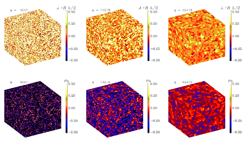
Figure 1: Visualizations of $\bm{A}\cdot\bm{B}\,\lambda/2$ (upper row) and $\mu_{5}$ (lower row) on the periphery of the computational domain for Run O at $\eta\approx 4600$ (left) 15,000 (middle), and 46,000 (right).

For $k_{0}\gg|\mu_{50}|$, on the other hand, we expect the following evolution of the system.

1. The system is frozen at $\eta<\eta_{\lambda}$.

2. The magnetic field evolves according to the inverse cascade at $\eta\simeq\eta_{\lambda}$ in a similar way as the usual inverse cascade for a nonchiral helical magnetic field,

   $$k_{\rm I}\propto\eta^{-2/3},\quad{\cal E}_{\rm M}\propto\eta^{-2/3},\quad\mbox{and}$$ (29)

   $$\langle\mu_{5}\rangle=-\langle\mu_{\rm M}^{+}\rangle+\langle\mu_{\rm M}^{-}\rangle=\mathrm{const},$$ (30)

   since the CME is not effective at $k\simeq k_{\rm I}$ so that the magnetic helicity and chirality are individually conserved. Since $k_{\rm I}$ decays, eventually it becomes smaller than $|\mu_{5}|$, and the system enters the regime similar to the previous case.

3. If the CPI does not sufficiently amplify the negative helicity modes, the CME becomes effective at $\eta\simeq\eta_{\mathrm{ACC}}$ $(>\eta_{\lambda})$, which is now evaluated as

   $$\eta_{\mathrm{ACC}}\equiv\frac{\sigma^{3}}{|\mu_{50}|^{3}k_{0}^{3}}\eta_{\lambda}^{-2}\simeq\frac{2\sigma^{3}}{{\bar{\rho}}\lambda\mu_{50}^{2}}.$$ (31)

   Here, we have used Eq. (25) and $k_{\rm I}(\eta)=k_{0}(\eta/\eta_{\lambda})^{-2/3}$, as well as Eq. (14). When $\eta>\eta_{\mathrm{ACC}}$ we have the inverse cascade with the conservation of the adapted Hosking integral,

   $$k_{\rm I}\propto\eta^{-4/9},\quad{\cal E}_{\rm M}\propto\eta^{-10/9},\quad\mbox{and}$$ (32)

   $$\langle\mu_{5}\rangle=-\langle\mu_{\rm M}^{+}\rangle+\langle\mu_{\rm M}^{-}\rangle\propto\eta^{-2/3}.$$ (33)

   Note that in this case, the CPI would not grow much due to the earlier onset of the chirality decay.

The assumption of inefficient CPI is guaranteed if the mild hierarchy $|\mu_{5}|\gtrsim k_{\text{I}}$ at $\eta_{\mathrm{CPI}}$ or $\eta_{\mathrm{ACC}}$ still holds. However, we have $|\mu_{5}|/k_{\text{I}}|_{\eta_{\mathrm{CPI}}}=(2\sigma^{2}/{\bar{\rho}}\lambda)^{1/3}$, which is ${\cal O}(10^{2})$ for the plasma of the Standard Model (SM) of particle physics with $\alpha\simeq 10^{-2}$ and $g_{*}\simeq 10^{2}$. In this case, there is a relatively large hierarchy between the chiral chemical potential and the peak scale of the magnetic field. We then might expect an earlier onset of the chirality decay triggered by the CPI. Namely, we have another possibility of the scaling law, which is a modification of step 3 discussed above, so we refer to it as step $3^{\prime}$, i.e.,

1. After some epoch of the onset of CPI,

   $$\eta\simeq\eta_{5\mathrm{dec}}=c_{A}\,\eta_{\mathrm{CPI}},\quad\text{with}\quad c_{A}=\mathcal{O}(10),$$ (34)

   the system enters the regime of the ACC. If the conservation of the adapted Hosking integral, with the rapid communication between the chirality and helicity through the CME, governs the evolution of the system, we would still have the scaling laws Eqs. (32) and (33), but the evolution nevertheless would have relatively large uncertainty, because of the exponential instability from the CPI. For later purposes, we keep the ambiguity in the scaling evolution and introduce a scaling index $q_{5}$ such that

   $$\langle\mu_{5}\rangle=-\langle\mu_{\rm M}^{+}\rangle+\langle\mu_{\rm M}^{-}\rangle\propto\eta^{-q_{5}},$$ (35)

   which will be used in Sec. IV.

In Table LABEL:TAnalyticTimeScale, we summarize the characteristic time scales relevant for the evolution of the system; see Appendix A for a summary of additional time scales and wave numbers defined in this paper.

Some of the features described above will be confirmed by direct numerical simulations in Sect. III. They can have important consequences for baryon production, as will be discussed at the end of the paper.

III Results

In this section, we show the results of the direct numerical simulation. We first study the case with $k_{0}\ll|\mu_{50}|$ until Sec. III.7. In Sec. III.8 we study the case with $k_{0}\gg|\mu_{50}|$. Some of our observations will turn out to be consistent with the theoretical prediction discussed in Sec. II.5. We will also see some other features that have not been addressed there.

III.1 Visualization of magnetic and fermion chiralities

We begin by discussing the simulation of Ref. Brandenburg et al. (2023) with $k_{0}\ll|\mu_{50}|$, which we refer to as Run O. In Fig. 1, we present visual impressions of magnetic and fermion chiralities in Run O at different times. We see that the turbulent structures gradually grow in size and the extreme values away from zero decrease as time goes on. Furthermore, $\mu_{5}$ and $\bm{A}\cdot\bm{B}\,\lambda/2$ have predominantly opposite signs, as expected. Locally, however, there is no correspondence between the two fields. This is because the vanishing total chirality is only a statistical property.

III.2 Evolution of characteristic scales

As discussed in Ref. Brandenburg et al. (2023), it is important to allow for sufficient scale separation between the smallest available wave number $k_{1}\equiv 2\pi/L$ and the initial wave number of the peak, $k_{0}$. It is also important that there is enough separation between $k_{0}$ and the initial wave number of the CPI, $|\mu_{50}|/2$, to confirm distinct features of the evolution of the system. Both, $k_{0}$ and $|\mu_{50}|/2$, in turn, must be much smaller than the largest available wave number $k_{\rm Ny}=k_{1}N/2$. Sufficient scale separation between $k_{1}$ and $k_{0}$ is particularly important for obtaining the theoretically expected increase of $\xi_{\rm M}\propto\eta^{4/9}$ along with the decay of ${\cal E}_{\rm M}\propto\eta^{-10/9}$, based on the conservation of the Hosking integral adapted to the total chirality. Indeed, in Run O, an optimized balance between the two scale separation requirements has been achieved.

With the start of the simulation, the helical random magnetic field, which is present initially, drives turbulent motions through the Lorentz force. This causes $E_{\rm K}(k)$ to grow quickly at all wave numbers, but it is always less than $E_{\rm M}(k)$; see Fig. 2, where we compare kinetic and magnetic energy spectra at different times. After some time, $E_{\rm K}(k)$ approaches $E_{\rm M}(k)$ at large values of $k$, i.e., the motions are in approximate equipartition with the magnetic field at high wave numbers. This observation supports the estimate of $u_{\rm rms}^{\mathrm{max}}$ for ${\tilde{v}}_{\lambda}$; see Eq. (14). At the same time, the initial $k^{-5/3}$ spectrum for $E_{\rm M}(k)$ develops into a slightly steeper one due to finite magnetic diffusion. In Fig. 2, we also mark the two scale separation ratios.

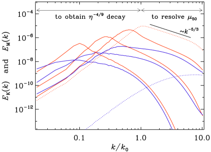
Figure 2: Magnetic energy (red lines) and kinetic energy (blue lines) spectra for Run O at times $\eta=460$, 4600, and 46,000. The dotted lines denote the earliest outputted time $\eta=0.3$. The straight black line indicates the initial $k^{-5/3}$ spectrum for the magnetic field. In the upper part, the two-sided arrows indicate the requirements for scale separation at small and large $k$ to obtain the $k_{\rm p}\propto\eta^{-4/9}$ decay and to resolve $|\mu_{50}|$, respectively.

As already discussed in Ref. Brandenburg et al. (2023), even though there is vanishing net chirality, $\langle\mu_{\rm M}\rangle+\langle\mu_{5}\rangle=0$, there is still some degree of inverse cascading, just like in nonhelical magnetically dominated turbulence (Brandenburg et al., 2015; Brandenburg and Kahniashvili, 2017). We see this clearly in Fig. 3, where the position of the magnetic peak, $k_{\rm I}(\eta)$, gradually moves to smaller values. At the same time, the height of the peak decreases, following an approximate power law $\propto k^{\beta}$, with $\beta=3/2$; see Fig. 3. This can be explained by the conservation of the Hosking integral Hosking and Schekochihin (2021); Zhou et al. (2022); see also Eq. (23). The exponent $\beta=3/2$ is characteristic of the fact that the net chirality vanishes, even though near the peak itself the field is locally fully helical, as we see from the proximity of $k|H_{\rm M}(k)|/2$ and ${\cal E}_{\rm M}(k)$; see Eq. (16).

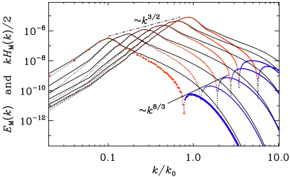
Figure 3: Magnetic energy (solid lines) and normalized helicity spectra $kH_{\rm M}(k)/2$ (dotted lines with red and blue symbols for positive and negative helicity spectra, respectively) for Run O at times $\eta=150$, $460$, 1500, 4600, 15,000, and 46,000. The peaks $k_{\mathrm{I}}$ (peaks of the red curves) and $k_{\mathrm{II}}$ (peaks of the blue curves) evolve underneath the envelopes $\propto k^{3/2}$ and $\propto k^{8/3}$, respectively.

The newly injected magnetic helicity from the CPI leads to a growth of the magnetic field at large wave numbers. It manifests itself mostly through the build-up of negative magnetic helicity at high wave numbers. At some point, we also see a gradual propagation of the secondary peak $k_{\rm II}$ toward smaller $k$, which has not been addressed in Sec. II.5. It lies underneath an envelope with an approximate $k^{8/3}$ slope; see Fig. 3. At present, the exponent 8/3 is just empirical and there is no theory for it. It should be noted, however, that in other cases with a shorter inertial range, we have found larger exponents. Thus, the exponent could also be smaller when the inertial range is larger, i.e., when there is more scale separation and $\langle\mu_{5}\rangle\xi_{\rm M}$ is larger.

Another characteristic wave number is $k_{\pm}$, where the sign of the spectral magnetic helicity changes. It is used in the definitions of $\langle\mu_{\rm M}^{+}\rangle$ and $\langle\mu_{\rm M}^{-}\rangle$ in Eqs. (18) and (19).

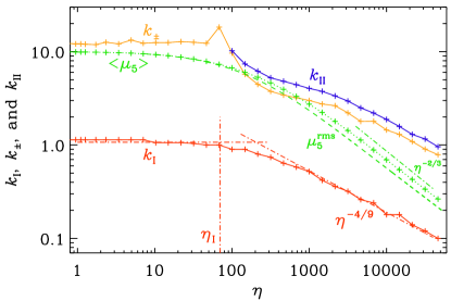
Figure 4: Comparison of $k_{\rm I}$ (red), $k_{\pm}$ (orange), and $k_{\rm II}$ (blue) for Run O. The green dashed line shows $\langle\mu_{5}\rangle$ and the green dotted line shows the rms value $\mu_{5}^{\rm rms}$. The sloping red (green) dashed-dotted line indicates $\eta^{-4/9}$ ($\eta^{-2/3}$) scaling.

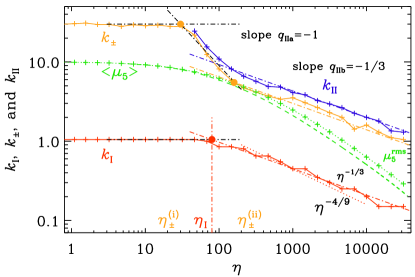
Figure 5: Similarly to Fig. 4, but for Run I. The red dashed-dotted line indicates here the $\eta^{-1/3}$ scaling, which describes the $k_{\rm I}$ scaling better than the $\eta^{-4/9}$ scaling indicated by the red dotted line. The orange and red dots indicate the crossings of the extrapolated tangents on which the times $\eta_{\pm}^{\mathrm{(i)}}$, $\eta_{\mathrm{I}}$, and $\eta_{\pm}^{\mathrm{(ii)}}$ are based.

Table 2: Summary of the runs discussed in this paper. Except for Run P, where $\lambda=500$, we have in all other cases $\lambda=2\times 10^{4}$. Runs A and B below the last horizontal line have nonvanishing net chirality and are discussed at the end of the paper. The asterisk on the value of $k_{1}=0.01$ Run J” indicates that the resolution is $N^{3}=2048^{3}$, so the Nyquist wave number is here the same as for Run J’ with $k_{1}=0.02$.

Run $k_{0}$ $-\mu_{50}$ $\sigma^{-1}$ SLD $\eta_{\rm CPI}$ $\eta_{\rm diff}$ $\eta_{\mu_{\mathrm{M}}^{+}}$ $q_{\rm I}$ $\eta_{\rm flip}$ $\eta_{\pm}^{\mathrm{(i)}}$ $\eta_{\mathrm{I}}$ $\eta_{\pm}^{\mathrm{(ii)}}$ $\eta_{\mu_{\mathrm{M}}^{-}}$ $|\langle\mu_{\rm M}^{-}\rangle|^{\max}$ $k_{\pm}/k_{\rm I}$ $k_{\rm II}/k_{\rm I}$ $v_{\lambda}$ $u_{\rm rms}^{\max}$ $k_{1}$ VI 1 160 $5\times 10^{-4}$ no 0.08 $2\times 10^{3}$ 3 1/3 — 0.3 45 14 7 43 1.4 2.0 1.13 0.095 0.2 V 1 80 $5\times 10^{-4}$ no 0.3 $2\times 10^{3}$ 4 1/3 — 0.5 55 40 4 13 1.5 1.8 0.57 0.050 0.2 IV 1 50 $5\times 10^{-4}$ no 0.8 $2\times 10^{3}$ 6 1/3 — 1.6 50 55 50 5.1 1.5 2.0 0.35 0.050 0.1 III 1 30 $5\times 10^{-4}$ no 2.2 $2\times 10^{3}$ 14 1/3 — 1.7 80 108 150 1.5 1.8 2.3 0.21 0.018 0.2 II+ 1 20 $5\times 10^{-4}$ no 5 $2\times 10^{3}$ 18 1/3 — 6 75 160 200 0.46 1.8 3.1 0.141 0.031 0.1 II 1 20 $2\times 10^{-4}$ no 12.5 $5\times 10^{3}$ 60 1/3 — 9 75 120 200 0.009 4.4 6.7 0.141 0.032 0.1 II$-$ 1 20 $1\times 10^{-4}$ no 25 $1\times 10^{4}$ 160 1/3 — 14 75 140 200 0.003 6.7 10 0.141 0.031 0.1 I 1 10 $2\times 10^{-4}$ no 50 $5\times 10^{3}$ 125 1/3 — 30 80 160 250 0.009 6.7 9.6 0.071 0.030 0.05 O 1 10 $2\times 10^{-4}$ no 50 $5\times 10^{3}$ 125 4/9 — 20 70 120 300 0.008 8.1 9.6 0.071 0.0123 0.02 O’ 1 10 $2\times 10^{-4}$ yes 50 $5\times 10^{3}$ 125 4/9 — 20 110 120 400 0.015 6.4 8.4 0.071 0.0103 0.02 L 1 10 $2\times 10^{-4}$ yes 50 $5\times 10^{3}$ 125 4/9 — 180 400 500 1000 0.027 6.7 8.7 0.071 0.0079 0.01 M 1 7 $2\times 10^{-4}$ yes 102 $5\times 10^{3}$ 165 1/3 — 260 220 800 800 0.006 5.8 7.2 0.049 0.0065 0.01 N 1 5 $2\times 10^{-4}$ yes 200 $5\times 10^{3}$ 235 1/3 — 350 200 800 1000 0.0015 6.3 7.8 0.035 0.0055 0.01 N’ 1 5 $2\times 10^{-4}$ yes 200 $5\times 10^{3}$ 200 4/9 — — 800 3000 15000 0.00004 5.5 2.4 0.035 0.0035 0.005 F 1 5 $2\times 10^{-4}$ yes 200 $5\times 10^{3}$ — 4/9 100 — 250 9000 — — 30 30 0.035 0.0055 0.01 J 1 5 $5\times 10^{-4}$ no 80 $2\times 10^{3}$ 71 4/9 — 230 300 500 700 0.0003 6.1 7.6 0.035 0.0068 0.01 J” 1 5 $5\times 10^{-4}$ no 80 $2\times 10^{3}$ 71 4/9 — 90 300 500 460 0.0006 6.1 7.6 0.035 0.0071 0.01* J’ 1 5 $5\times 10^{-4}$ no 80 $2\times 10^{3}$ 76 1/3 — 95 120 500 460 0.0005 5.8 7.7 0.035 0.0070 0.02 P 1 0.1 $2\times 10^{-4}$ no $5\times 10^{5}$ $5\times 10^{3}$ $10^{4}$ 3/5 — – 160 — — $3\times 10^{-9}$ — — 0.001 0.0070 0.02 G 0.5 10 $2\times 10^{-4}$ no 50 $2\times 10^{4}$ 200 1/3 — 30 360 360 300 0.044 4.6 6.6 0.071 0.0188 0.05 H 0.2 10 $2\times 10^{-4}$ no 50 $1.2\times 10^{5}$ 375 1/3 — 75 2000 2000 3000 0.42 2.0 2.7 0.071 0.0074 0.02 A 1 10 $2\times 10^{-4}$ no 50 $5\times 10^{3}$ — 4/9 — 8 110 210 — — 7.3 9.5 0.071 0.0109 0.02 B 1 10 $2\times 10^{-4}$ no 50 $5\times 10^{3}$ — 4/9 — 20 90 120 250 — 7.8 8.9 0.071 0.0137 0.02

In Fig. 4, we plot the evolution of the characteristic wave numbers $k_{\rm I}$, $k_{\pm}$, and $k_{\rm II}$. We clearly see the $k_{\rm I}\propto\eta^{-4/9}$ decay predicted by the conservation of the Hosking integral adapted to the total chirality Brandenburg et al. (2023). It emerges after a time $\eta_{\rm I}$, which is expected to be close to $\eta_{\lambda}$ (and also $\eta_{\mathrm{turb}}$); see Eq. (15). In Run O we find $\eta_{\rm I}\approx 100$.

The evolution of $k_{\pm}$ and $k_{\rm II}$ can be seen more clearly when the Nyquist wave number is larger. We therefore discuss in Fig. 5 another run, also with $N=1024^{3}$ mesh points, but now with $k_{1}=0.05$ (instead of 0.02), so $k_{\rm Ny}=25.6$, which is a little over five times larger than $|\mu_{\rm 50}|/2=5$. In Table LABEL:Ttimescales, this run is referred to as Run I, which differs from the previously discussed Run O mainly in the value of $k_{1}$. It also has a shallower scaling of the correlation length, $\xi_{\rm M}\propto k_{\mathrm{I}}^{-1}\propto\eta^{1/3}$, which seems to be an artifact caused by insufficient scale separation, i.e., the value of $k_{1}$ is not sufficiently small. Empirically, we find that, if $k_{0}/k_{1}\gg 20$, there is an inverse cascade with $\xi_{\rm M}\propto k_{\mathrm{I}}^{-1}\propto\eta^{4/9}$. The parameters $\eta_{\mathrm{I}}$, $\eta_{\pm}^{\mathrm{(i)}}$, and $\eta_{\pm}^{\mathrm{(ii)}}$, listed in Table LABEL:Ttimescales, are discussed below. We also give here the values of $v_{\mu}$ and $v_{\lambda}/v_{\mu}$. Run O’ is similar to Run O, except that here, SLD has been added. The two runs are virtually indistinguishable.

The evolution of the peaks of the spectrum can be summarized as follows. (i) After the start of the run, the CPI induces a growth of the negative helicity modes at the secondary peak $k_{\mathrm{II}}$, which stays constant until $\eta=\eta_{\pm}^{\mathrm{(i)}}$, and then starts to decrease with time in a power law fashion, $k_{\mathrm{II}}\propto\eta^{-q_{\rm IIa}}$, with $q_{\rm IIa}\approx 1$ in all cases. (ii) The original large-scale spectrum is unchanged until some time $\eta=\eta_{\rm I}$ and then starts to decrease via an inverse cascade with $k_{\mathrm{I}}(\eta)\propto\eta^{-q_{\rm I}}$, where $q_{\rm I}$ is expected to be equal to the exponent $q=4/9$ found in Ref. Brandenburg et al. (2023). (iii) At time $\eta=\eta_{\pm}^{\mathrm{(ii)}}$, the decay of the secondary peak becomes slower with a smaller index, $k_{\mathrm{II}}\propto\eta^{-q_{\rm IIb}}$, with $q_{\rm IIb}<q_{\rm IIa}\approx 1$. Those parameters are summarized in Table LABEL:Ttimescales.

The plot of characteristic wave numbers $k_{\rm I}$, $k_{\pm}$, and $k_{\rm II}$ in Fig. 5 shows three distinct times, $\eta_{\pm}^{\rm(i)}\mathrel{\mathchoice{\vbox{\offinterlineskip\halign{\hfil$\displaystyle#$\hfil\cr<\cr\sim\cr}}}{\vbox{\offinterlineskip\halign{\hfil$\textstyle#$\hfil\cr<\cr\sim\cr}}}{\vbox{\offinterlineskip\halign{\hfil$\scriptstyle#$\hfil\cr<\cr\sim\cr}}}{\vbox{\offinterlineskip\halign{\hfil$\scriptscriptstyle#$\hfil\cr<\cr\sim\cr}}}}\eta_{\rm I}\mathrel{\mathchoice{\vbox{\offinterlineskip\halign{\hfil$\displaystyle#$\hfil\cr<\cr\sim\cr}}}{\vbox{\offinterlineskip\halign{\hfil$\textstyle#$\hfil\cr<\cr\sim\cr}}}{\vbox{\offinterlineskip\halign{\hfil$\scriptstyle#$\hfil\cr<\cr\sim\cr}}}{\vbox{\offinterlineskip\halign{\hfil$\scriptscriptstyle#$\hfil\cr<\cr\sim\cr}}}}\eta_{\pm}^{\rm(ii)}$, where $k_{\pm}$ begins to decrease first rapidly, at $\eta=\eta_{\pm}^{\rm(i)}$, and later, at $\eta=\eta_{\pm}^{\rm(ii)}$, more slowly, approximately like $\eta^{-4/9}$, i.e., $q_{\rm IIb}\approx q=4/9$. The decay of $k_{\rm II}$ closely follows that of $k_{\pm}$. The decay of $k_{\rm I}$, on the other hand, does not show the rapid decay phase that we see in $k_{\pm}$ and $k_{\rm II}$, but turns directly into the approximate $\eta^{-4/9}$ decay at $\eta=\eta_{\pm}^{\rm(i)}$.

III.3 Onset of inverse cascading

It is of interest to vary the separation between $|\mu_{50}|/2$ and $k_{0}$ to see the dependence of the relevant characteristic times on these wave numbers. We have performed simulations for different values and consider runs where we change $k_{0}$ and keep $\mu_{50}$ fixed, and others where we change $\mu_{50}$ and keep $k_{0}$ fixed. It both cases, of course, since we want to satisfy $\langle\mu_{5}\rangle+\langle\mu_{\rm M}\rangle={\rm const}{}$, we need to adjust the amplitude of the initial magnetic field correspondingly. The results are summarized in Table LABEL:Ttimescales and plotted in Figs. 6 and 7.

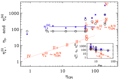
Figure 6: Dependence of $\eta_{\pm}^{\rm(i)}$, $\eta_{\rm I}$, and $\eta_{\pm}^{\rm(ii)}$ on $\eta_{\rm CPI}$. $\eta_{\pm}^{\rm(i)}$ shows an approximate $\eta_{\rm CPI}^{2/3}$ dependence along two branches that are separated by a factor of about 6. $\eta_{\rm I}$ and $\eta_{\pm}^{\rm(ii)}$ are essentially independent of $\eta_{\rm CPI}$. The inset shows that $\eta_{\pm}^{\rm(i)}$ scales inverse quadratically with $|\mu_{50}|$.

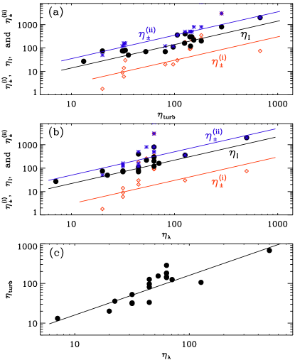
Figure 7: Dependence of $\eta_{\rm I}\approx\eta_{\pm}^{\mathrm{(ii)}}$ and $\eta_{\pm}^{\mathrm{(i)}}$ on (a) $\eta_{\rm turb}$ and (b) $\eta_{\lambda}$, as well as (c) the dependence of $\eta_{\rm turb}$ on $\eta_{\lambda}$.

One may presume that $\eta_{\pm}^{\mathrm{(i)}}$ is roughly estimated by $\eta_{\mathrm{CPI}}$ since the grow of negative helicity modes becomes effective at that time. We see, however, that, while $\eta_{\pm}^{\rm(i)}$ decreases quadratically with increasing $|\mu_{50}|$, the dependence on $\eta_{\rm CPI}=\sigma\mu_{50}^{-2}$ is shallower than linear and follows approximately an $\eta_{\rm CPI}^{2/3}$ scaling; see Fig. 6. Thus, $k_{\rm II}$ starts to decline more rapidly when $|\mu_{50}|$ is large, although it is unclear why this exponent is here $\approx 2/3$. On the other hand, we see that the five data points with $k_{1}=0.01$ (Runs L, M, N, J, and J” with smaller $|\mu_{50}|$) lie on another $\eta_{\rm CPI}^{2/3}$ line that is shifted upward by a factor of about 6 relative to the runs with larger $k_{1}$. The reason for this is that for large values of $\eta_{\rm CPI}$, it became necessary to decrease the value of $k_{1}$. This decreased the Nyquist wave number since $N$ remained unchanged, which can cause artifacts in the values of $k_{\pm}$. Small values of $k_{1}$ also facilitates the $\eta^{4/9}$ scaling of $\xi_{\rm M}$ and related length scales; see the comparison between Runs N and N’ in Table LABEL:Ttimescales. This shows that $\eta_{\pm}^{\rm(i)}$ is currently very sensitive to these restrictions which will be alleviated in future with larger computational power. Nevertheless, there is clearly a trend for an uprise in the dependence of $\eta_{\pm}^{\rm(i)}$ on $\eta_{\rm CPI}$ for large values.

Next, we examine the dependence of $\eta_{\mathrm{I}}$ and $\eta_{\pm}^{\mathrm{(ii)}}$ on $k_{0}$ and $\mu_{50}$. Figure 6 shows that the time $\eta_{\rm I}$ of the onset of the decline of $k_{\rm I}$ does not strongly depend on the value of $\mu_{50}$. Likewise, the time $\eta_{\pm}^{\mathrm{(ii)}}$ when the decay of $k_{\rm II}$ slows down, does not strongly depend on $\mu_{50}$. Again, however, there is an upward shift of data points for the four runs, for which $k_{1}=0.01$. As discussed in Sec. II.5, we expect that $\eta_{\mathrm{I}}$ is close to $\eta_{\mathrm{turb}}$ and $\eta_{\lambda}$. The upper two panels of Fig. 7 show the dependence of $\eta_{\pm}^{\rm(i)}$, $\eta_{\rm I}$, and $\eta_{\pm}^{\rm(ii)}$ on $\eta_{\mathrm{turb}}$ and $\eta_{\lambda}$, respectively. From these plots, we estimate that

$$\eta_{\rm I}\approx 1.4\,\eta_{\rm turb}\approx 2.2\,\eta_{\lambda}.$$ (36)

In the lowest panel of Fig. 7, we also show the relation between $\eta_{\rm turb}$ and $\eta_{\lambda}$, i.e.,

$$\eta_{\mathrm{turb}}\approx 1.6\,\eta_{\lambda},$$ (37)

which shows the validity of the estimate of $u_{\rm rms}^{\mathrm{max}}$ in terms of ${\tilde{v}}_{\lambda}$. Equation (36) is useful for estimating the properties of magnetic field strength and coherence length at later times. Therefore, we conclude that the numerical results support, at least for a moderate scale separation, $1<|\mu_{50}|/k_{0}\lesssim{\cal O}(10)$, the theoretical estimate for the evolution of the characteristic scales given in Sec. II.5 with a more accurate determination of the time of the onset of the scaling evolution, Eq. (36).

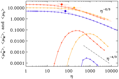
Figure 8: Comparison of $\langle\mu_{\rm M}^{\pm}\rangle$ for Run II (red lines), Run J (blue lines), and Run G (orange lines). The times $\eta_{\rm ACC}$ are marked by the correspondingly colored filled symbol at the crossing points of the extrapolated $\eta^{-2/3}$ decay law with the initially constant values, indicated by dotted line. The $\eta^{-4/3}$ decay law $\langle\mu_{\rm M}^{-}\rangle$ is shown as the dashed-dotted line.

III.4 Evolution of $\langle\mu_{5}\rangle$ and $\langle\mu_{\rm M}^{\pm}\rangle$

We now discuss how the chirality of the system evolves. Using Eqs. (18) and (19), we divide the magnetic helicity into $\langle\mu_{\rm M}^{+}\rangle$ and $\langle\mu_{\rm M}^{-}\rangle$. The typical evolution of $\langle\mu_{5}\rangle$ and $\langle\mu_{\rm M}^{\pm}\rangle$ is as follows. (i) $\langle\mu_{5}\rangle$ and $\langle\mu_{\rm M}^{+}\rangle$ stay constant until the time $\eta=\eta_{\mu_{\mathrm{M}}^{+}}$, when the ACC commences exhibiting a power law decay. (ii) $\langle\mu_{\rm M}^{-}\rangle$ grows until the time $\eta=\eta_{\mu_{\mathrm{M}}^{-}}$ and then decays. Thus, $\eta_{\mu_{\mathrm{M}}^{-}}$ is determined as the time when $\langle\mu_{\rm M}^{-}\rangle$ is maximum.

As discussed in Sec. II.5, the decay of $\langle\mu_{5}\rangle$ and $\langle\mu_{\rm M}^{+}\rangle$ due to the ACC is expected to be like $\eta^{-2/3}$. In Fig. 8, we have overplotted the asymptotic $\eta^{-2/3}$ decay laws of magnetic helicity with results of some of the representative numerical runs (Runs II, J, and G), which clearly shows that the numerical results support the theoretical prediction.

The decay of $\langle\mu_{\rm M}^{-}\rangle$ is faster than that of $\langle\mu_{5}\rangle$ and $\langle\mu_{\rm M}^{+}\rangle$ and follows an approximate $\eta^{-4/3}$ law, resulting in a decay of the ratio $\langle\mu_{\rm M}^{-}\rangle/\langle\mu_{\rm M}^{+}\rangle\propto\eta^{-2/3}$. Therefore, unless $\langle\mu_{\rm M}^{-}\rangle$ becomes comparable to $\langle\mu_{\rm M}^{+}\rangle$ when the grow stops, a complete cancellation between $\langle\mu_{\rm M}^{-}\rangle$ and $\langle\mu_{\rm M}^{+}\rangle$ never occurs.

The production of $\langle\mu_{\rm M}^{-}\rangle$ is expected to be a result of the CPI. We now address the question of how much $\langle\mu_{\rm M}^{-}\rangle$ is being produced and what its maximum value depends on. Figure 8 shows that $\langle\mu_{\rm M}^{-}\rangle$ is generally rather small, and at least for $\mu_{50}/k_{0}\lesssim 20$ there is always a strong imbalance between $|\langle\mu_{\rm M}^{+}\rangle|$ and $|\langle\mu_{\rm M}^{-}\rangle|$, which never enters a phase with a near-complete cancellation.

To see whether this is related to the value of the conductivity, we compare simulations with different values of $\sigma$. It turns out that runs with smaller magnetic diffusivity ($\sigma^{-1}=10^{-4}$) result in an even larger imbalance, while those with a larger diffusivity ($\sigma^{-1}=5\times 10^{-4}$) have a smaller imbalance; compare Runs II$+$, II, and II$-$ in Table LABEL:Ttimescales.

Before closing this section, let us comment on another trend in the numerical runs we conducted regarding the absence of a near-complete cancellation between $\langle\mu_{\rm M}^{-}\rangle$ and $\langle\mu_{\rm M}^{+}\rangle$. For Runs III–VI, the ratio $|\langle\mu_{\rm M}^{-}\rangle|^{\max}/|\mu_{50}|$ becomes rather large. This could be due to the very large scale separation of $k_{0}$ and $|\mu_{50}|$. This suggests a possibility that the CPI completes the cancellation between the magnetic helicity and chirality immediately. However, the positive and negative helicity modes are distributed at separate length scales with the negative ones sitting at higher length scales and the latter receives a stronger magnetic diffusion. Therefore we expect the cancellation not to be complete and that the two helicity modes decay with a power-law decay, not an exponential one, though the scaling index can be different from $-2/3$. In order to investigate the evolution of the system in such extreme cases, $|\mu_{50}|/k_{0}\gg{\cal O}(10)$, we need to have a sufficiently large box size to realize the corresponding scale separation. The detailed study is left for future study.

III.5 Onset of ACC

In Fig. 9, we show the dependence of $\eta_{\mu_{\mathrm{M}}^{+}}$ and $\eta_{\mu_{\mathrm{M}}^{-}}$ on $\eta_{\mathrm{ACC}}=\sigma/|\mu_{50}k_{0}|$ (for the case $k_{0}\ll|\mu_{50}|$; see Eq. (26)). It turns out that $\eta_{\mu_{\mathrm{M}}^{+}}$ increases with $\eta_{\mathrm{ACC}}=\sigma/|\mu_{50}k_{0}|$ such that

$$\eta_{\mu_{\mathrm{M}}^{+}}\approx 0.2\,\eta_{\rm ACC}=0.2\,\sigma/|\mu_{50}k_{0}|$$ (38)

provides a good description to the data, which supports the discussion in Sec. II.5, at least for a mild hierarchy $|\mu_{50}|\gtrsim k_{0}$. Furthermore, $\eta_{\mu_{\mathrm{M}}^{-}}$ shows an approximately linear dependence on $\eta_{\rm ACC}$. This is reasonable because the CPI becomes ineffective when the ACC onsets such that $\langle\mu_{\mathrm{M}}^{-}\rangle$ is no longer amplified by the CPI after that.

Figure 9: Dependence of $\eta_{\mu_{\mathrm{M}}^{+}}$ and $\eta_{\mu_{\mathrm{M}}^{-}}$ on (a) $\sigma/|\mu_{50}k_{0}|$ as well as the geometric means of $\eta_{\rm CPI}$ and (b) either $\eta_{\rm turb}$ or (c) $\eta_{\lambda}$.

III.6 The scale ratios $k_{\pm}/k_{\rm I}$ and $k_{\rm II}/k_{\rm I}$

We also mention another observation in the case with $k_{0}\ll|\mu_{50}|$. At late times, the scale ratios $k_{\pm}/k_{\rm I}$ and $k_{\rm II}/k_{\rm I}$ reach values that are approximately constant in time. It is about $10$ in the case of Run O, i.e., equal to the initial scale separation, $|\mu_{50}|/k_{0}=10$. One might have expected the scale ratios to increase with $|\mu_{50}|/k_{0}$. However, in all other cases, this ratio is smaller. Some of this might also be caused by one of the two scale separation constraints not being well enough obeyed, although the counter-intuitive trend remains surprising.

Figure 10: Dependence of $k_{\pm}/k_{\rm I}$ and $k_{\rm II}/k_{\rm I}$ on $\eta_{\rm CPI}$, showing an $\eta_{\rm CPI}^{-0.4}$ behavior. on $\eta_{\rm diff}$, showing a $\propto\eta_{\rm diff}^{1/2}$ behavior.

In Fig. 10, we show the ratios $k_{\pm}/k_{\rm I}$ and $k_{\rm II}/k_{\rm I}$ versus $|\mu_{50}|/k_{0}=(\eta_{\rm diff}/\eta_{\rm CPI})^{1/2}$. The two insets give separately the dependencies on $1/\eta_{\rm CPI}$, showing an $\eta_{\rm CPI}^{-0.4}$ behavior, and on $\eta_{\rm diff}$, with a $\propto\eta_{\rm diff}^{1/2}$ behavior. We see that $k_{\pm}/k_{\rm I}$ and $k_{\rm II}/k_{\rm I}$ decrease both with $1/\eta_{\rm CPI}$ and with $\eta_{\rm diff}$, giving a combined dependence on just the ratio $|\mu_{50}|/k_{0}$. Thus, we see that, somewhat unexpectedly, large $|\mu_{50}|$ and small $k_{0}$ tend to be detrimental to producing large scale ratios.

Figure 11: Evolution of $\langle\mu_{\rm M}\rangle$ (red), $\langle\mu_{5}\rangle$ (blue), and their sum (black) for Run F with $\eta_{\rm flip}=100$ and $\Gamma_{\rm f0}=10^{-2}$ either for the rest of the run or only until $\eta_{\rm off}=10^{3}$. The dotted lines correspond to Run N without spin flipping.

III.7 Effect of chirality-flipping

The simulations discussed so far had $\Gamma=0$ and they resulted in a final state where $\langle\mu_{5}\rangle$ and $\langle\mu_{\rm M}\rangle$ vanish at late times. As discussed in the introduction, spin flipping could prematurely lead to a vanishing $\langle\mu_{5}\rangle$, which would imply that the decay of $\langle\mu_{\rm M}\rangle$ would slow down and level off at a value away from zero. To study this quantitatively, we show in Fig. 11 the evolution of $\langle\mu_{5}\rangle$, $\langle\mu_{\rm M}\rangle$, and $\langle\mu_{5}\rangle+\langle\mu_{\rm M}\rangle$ for Run F with $\eta_{\rm flip}=100$ and $\Gamma_{\rm f0}=10^{-2}$ either for the rest of the run or only until $\eta_{\rm off}=10^{3}$ (Run F in Table LABEL:Ttimescales). We expect that if chirality flipping becomes effective much later than the ACC, we do not see the effect of chirality flipping, while if it becomes effective much earlier, we do not see the ACC. This is demonstrated in Appendix B, where we show spin-flipping versions of Runs VI and P, where $\eta_{\rm ACC}\ll\eta_{\rm flip}$ and $\eta_{\rm ACC}\gg\eta_{\rm flip}$, respectively. Thus we choose the parameter such that the chirality flipping becomes effective around (or somewhat before) the time of onset of the ACC to capture the behavior of the system at an intermediate stage.

First, we study a case where spin flipping acts permanently (after $\eta=\eta_{\rm flip}$), which is shown in Fig. 11 as solid lines. We see that $|\langle\mu_{5}\rangle|$ begins to decrease rapidly to zero after $\eta_{\rm flip}=100$. This slows down the decay of $\langle\mu_{\rm M}\rangle$, which then declines at a much smaller rate; compare with the evolution for Run N, which is similar to Run F, but without spin flipping. Qualitatively similar behaviors are also seen for smaller values of $\Gamma_{\rm f0}$. In all cases, we see that $\langle\mu_{5}\rangle+\langle\mu_{\rm M}\rangle$ evolves away from zero. This is because the total chirality is then no longer conserved. The decay of $\langle\mu_{\rm M}\rangle$ is understood by magnetic diffusion. Thus we expect the decrease to slow down for a larger scale separation between the magnetic diffusion scale and $k_{\rm I}$.

Next, it is also of interest to study a case where spin flipping acts only for a certain time interval and is then turned off again at $\eta=\eta_{\rm off}$. This case is shown in Fig. 11 as dashed lines. We see that, when $\Gamma=0$ after $\eta_{\rm off}=10^{3}$, the sum $\langle\mu_{5}\rangle+\langle\mu_{\rm M}\rangle$ is strictly constant and away from zero. This is in contrast to the case with permanently nonvanishing $\Gamma_{\rm f0}$, where the sum continues to decrease slowly. The constancy of the total chirality leads to the behavior that $\langle\mu_{\rm M}\rangle$ stops to decline rapidly at a larger value. Furthermore, during that time, some of the magnetic helicity decays due to the magnetic diffusion and is temporarily converted back into fermion chirality through the total chirality conservation; see the small increase of $\langle\mu_{5}\rangle$ with a positive maximum at $\eta\approx 4000$ in Fig. 11. Later, however, this excess fermion chirality gets converted back into magnetic fields, which explains the slight uprise of $\langle\mu_{\rm M}\rangle$ near the end of the simulation. Indeed, this process is similar to the one seen in Refs. Hirono et al. (2015); Schober et al. (2020). This is natural because after the decay of $\langle\mu_{5}\rangle$ the setup becomes very similar to the ones in these studies.

Figure 12: $k_{\pm}^{\mathrm{(i)}}$ and $k_{\rm I}$ for Run F with spin flipping, $\eta_{\rm flip}=100$ and $\Gamma_{\rm f0}=10^{-2}$ for the rest of the run. As in Fig. 4, the green dashed line shows $\langle\mu_{5}\rangle$ and the green dotted line shows $\mu_{5}^{\rm rms}$.

In Fig. 12, we show $\eta_{\pm}^{\mathrm{(i)}}$ and $\eta_{\rm I}$ in the presence of spin flipping. The results suggests that the $\eta^{-4/9}$ decay changes into the faster $\eta^{-2/3}$ decay. Spin flipping brings $\langle\mu_{5}\rangle$ close to zero. This process stops or slows down the decline of magnetic helicity, which therefore remains positive. At late times, $\langle\mu_{5}\rangle$, which was originally negative, now becomes positive and settles at a value of around $\langle\mu_{5}\rangle\approx k_{1}$. This is because at later times the positive chirality induced due to the helicity decay by the magnetic diffusion through the chiral anomaly is balanced by the erasure of the chirality through the CME Hirono et al. (2015); Schober et al. (2020), similar to the baryon asymmetry through the magnetic helicity decay much before the electroweak phase transition Giovannini and Shaposhnikov (1998a, b); Fujita and Kamada (2016).

The sign of the final value of $\langle\mu_{5}\rangle$ is determined by the magnetic helicity after the decay of $\langle\mu_{5}\rangle$ due to the onset of spin flipping. In the cases presented above, the sign of the magnetic helicity at the time of the onset of spin flipping was positive and thus the chiral chemical potential at later times was also positive. If the initial magnetic field is weaker and the total chirality being negative (see App. C), the sign of the final value of $\langle\mu_{5}\rangle$ can stay negative.

Our runs show that spin flipping can lead to a significant increase of the fraction of the magnetic helicity that can be preserved in spite of the fact that the system has vanishing total chirality. This also reduces the total energy density dissipation of the system. In the absence of spin flipping, both magnetic helicity and chiral chemical potential would approach zero, so there would be no magnetic helicity available for successful baryogenesis. In the real Universe, however, spin flipping due to the electron Yukawa interaction, which really violates the (total) chirality conservation, inevitably acts at $T\lesssim 10^{2}\,$TeV Campbell et al. (1992); Bödeker and Schröder (2019), and hence magnetic helicity survives more or less at the electroweak phase transition.

In Fig. 12, we see an interval between the onset of spin flipping, $\eta=\eta_{\mathrm{flip}}=10^{2}$, and the onset of the $\eta^{-2/3}$ scaling evolution of $k_{\rm I}$, $\eta\sim 6\times 10^{3}$, which marks the real onset of the evolution with (pure) magnetic helicity conservation. For a rough estimate of the magnetic field evolution, however, we shall practically use $\eta_{\mathrm{flip}}$ as the switching time between the adapted Hosking integral conservation and the (pure) magnetic helicity conservation.

III.8 Cases with initially small $|\mu_{50}|/k_{0}$

In all the cases considered so far, we assumed $|\mu_{50}|/k_{0}>1$. We now consider the opposite case and discuss runs with $\mu_{50}=-0.1$, keeping still $k_{0}=1$, so $|\mu_{50}|/k_{0}=0.1$ (Runs P, Q, and R), and also a run with $\mu_{50}=-0.5$ and $k_{0}=1$ (Run S). To prevent the magnetic field from being too weak, while still preserving vanishing total chirality, we decrease the value of $\lambda$ and choose $\lambda=500$, 50, and 5 for Runs  P (and S), Q, and R, respectively. All the runs end at $\eta\sim 10^{4}$. The parameters of these runs are summarized in Table LABEL:Tbeta. The magnetic diffusivity is taken as $\sigma^{-1}=2\times 10^{-4}$. In all our cases, the system does not even reach $\eta_{\mathrm{CPI}}$. This is because of the small value of $|\mu_{50}|$, which enters the CPI time inverse quadratically; see Eq. (10).

Table 3: Empirical values of $\beta$ for cases with $|\mu_{50}|<k_{0}$. For a given value of $\lambda$, the values of $v_{\rm A0}$ followed from the requirement that the total chirality vanishes. The resulting maximum rms velocity $u_{\rm rms}^{\max}$ is listed for completeness.

Run $-\mu_{50}$ $\lambda$ $v_{\mu}$ $\tilde{v}_{\lambda}$ $v_{\rm A0}$ $u_{\rm rms}^{\max}$ SLD $\beta$ $\eta_{\rm I}$ P 0.1 500 $2\times 10^{-5}$ 0.014 0.026 0.008 no 0.33 160 Q 0.1 50 $2\times 10^{-5}$ 0.045 0.081 0.028 no 0.15 50 R 0.1 5 $2\times 10^{-5}$ 0.141 0.257 0.076 yes 0.05 27 S 0.5 500 $10^{-4}$ 0.032 0.057 0.019 no 0.33 70

Table 4: Possible combinations of $q=2/(\beta+3)$, $p=2(1-q)$, and $r=p-q$ in the range $0\leq\beta\leq 1/3$.

$\qquad\beta$ $\qquad q$ $\qquad p$ $\qquad r$ $3/2=1.50$ $4/9\approx 0.44$ $10/9\approx 1.11$ $2/3\approx 0.67$ $1/3\approx 0.33$ $3/5=0.60$ $4/5=0.80$ $1/5=0.20$ $0.15$ $0.63$ $0.73$ $0.10$ $0.05$ $0.66$ $0.69$ $0.03$ $0$ $2/3=0.67$ $2/3=0.67$ $0$

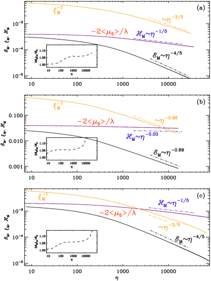
Figure 13: Time dependence of ${\cal E}_{\rm M}$ (black), $\xi_{\rm M}^{-1}$ (orange), ${\cal H}_{\rm M}$ (red), and $-2\langle\mu_{5}\rangle/\lambda$ (blue), for Runs P (a), R (b), and S (c).

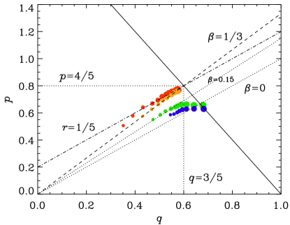
Figure 14: $pq$ diagram for Runs P (red symbols), S (orange symbols), Q (green symbols), and R (blue symbols) at times $t=700$, 1000, 1500, 2200, 3200, 4600, 6800, $10^{4}$, $1.5\times 10^{4}$, $1.5\times 10^{4}$, $2.2\times 10^{4}$, and $3.2\times 10^{4}$, corresponding to symbols of increasing size. The solid line denotes the scale-invariance line $p=2(1-q)$, the dashed line the empirical $\beta=1/3$ line, and the dashed-dotted line is the resulting $r=1/5$ line for the magnetic helicity decay. For stronger magnetic field strength (Runs Q and R), the solutions evolve along $\beta\approx 0.15$ and $\beta\approx 0.05$, respectively. Toward the end of the runs, the finite size effects of the domain begin to affect the solution. The dotted line denotes the $\beta=0$ line for magnetic helicity conservation and is shown for comparison.

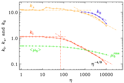
Figure 15: Comparison of $k_{\rm I}$ (red), $k_{\pm}$ (orange), and $k_{\rm II}$ (blue) for Run S with $\mu_{50}=-0.5$. The dashed-dotted line indicates $\eta^{-4/9}$. The green dashed line shows $\langle\mu_{5}\rangle$ and the green dotted line shows the rms value $\mu_{5}^{\rm rms}$.

Smaller values of $\lambda$ correspond to larger magnetic fields. We see that this also leads to a gradual decrease of the scaling index of the envelope of the magnetic energy spectrum, $\beta$; see Fig. 3. For a given value of $\beta$, we expect that the scaling indices $q$, $p$, and $r$, for the evolution of the magnetic coherence length ($\xi_{\rm M}\propto\eta^{q}$), energy density (${\cal E}_{\rm M}\propto\eta^{-p}$), and helicity (${\cal H}_{\rm M}\propto\eta^{-r}$), respectively, are given as $q=2/(\beta+3)$, $p=2(1-q)$, and $r=p-q$. In Fig. 13(a), we see that for Run P the exponents in agree reasonably well with those expected for $\beta=1/3$. In Fig. 13(b), we also show the results for Run R, where $\lambda$ is a hundred times smaller and the magnetic field ten times stronger. Now the value of $\beta$ is very small (about 0.05), corresponding to $q=0.66$, $p=0.69$, and $r=0.03$. Finally, Fig. 13(c) gives the results for Run S, where $\lambda=500$ is the same as for Fig. 13(a), but now $\mu_{50}=-0.5$ instead of $-0.1$. In this case, similarly to Run P, $\beta\approx 1/3$, $p\approx 4/5$, $q\approx 3/5$, and $r\approx 1/5$.

In Table LABEL:Tpqr, we list several combinations of the expected scaling indices $q$, $p$, and $r$ for $0\leq\beta\leq 3/2$. Interestingly, in the range $0\leq\beta\leq 1/3$, the values of $q$ and $p$ do not vary much in this range, especially compared to the case for the evolution with the (adapted) Hosking integral conservation, $\beta=3/2$, so if they do not agree with those from the simulations, the discrepancy cannot easily be resolved by changing the value of $\beta$ within reasonable limits. Note that $\beta=0$ is expected if the evolution is governed by (pure) magnetic helicity conservation.

In the corresponding $pq$ diagram Fig. 14, we see that all the runs approach the scale-invariance line $p=2(1-q)$. For Run P, it evolves along the line $r=1/5$. At the intersection, we have $q=3/5$ and $p=4/5$. However, for Runs Q and R with stronger magnetic field strengths, expressed in terms of the initial Alfvén speed $v_{\rm A0}=B_{0}/\sqrt{\rho_{0}}$ (which is well approximated by $\tilde{v}_{\lambda}$), the solution approaches the $\beta=0$ line, which suggests better conservation of magnetic helicity. Note that near the end of those runs, the data points may not be reliable because of the finite size of the domain. In addition, because of the stronger magnetic field, the Alfvén time is shorter and therefore $k_{\rm I}$ reaches $k_{1}$ more quickly. In any case, it is likely that for small $|\mu_{50}|/k_{0}$, we see an new stage of the evolution of the system where the magnetic helicity and chirality are temporarily conserved individually, as discussed in Sec. II.5. This is supported by the fact that the theoretically predicted time of the onset of ACC (or even CPI) should come much later, well after the end of the run; see Eqs. (10) and (31). In other words, from the present simulation results, we cannot distinguish between the two possible theoretical predictions for the later evolution in the case $k_{0}>|\mu_{50}|$; see steps 3 or $3^{\prime}$ given in Sec. II.5.

For all the simulations where initially $|\mu_{50}|<k_{0}$, we find that $\mu_{5}$ decays more slowly than $k_{\rm I}$; see Fig. 15 for Run S, as an example, where we see the crossing of $\mu_{5}$ and $k_{\rm I}$. The same is also seen for $|\mu_{50}|=0.1$, but then the crossing of $|\mu_{5}|$ and $k_{\rm I}$ occurs much later and is therefore not yet prominent. Again, these observations suggest that the magnetic helicity-conserving phase is an intermediate one before the solution resumes the decay governed by the adapted Hosking integral, as discussed in Sec. II.5.

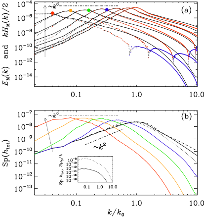
Figure 16: (a) Magnetic energy and (b) total helicity variance spectra at $t=70$ (dashed), $200$ (solid), $700$ (dotted), $2\times 10^{3}$ (blue), $7\times 10^{3}$ (green), $2\times 10^{4}$ (orange), and $7\times 10^{4}$ (red) for Run S. In (a), note that the $E_{\rm M}(k,t)$ evolve underneath a $k^{1/3}$ envelope, and the upward arrow indicates the sense of time. In (b), the slopes $k^{2}$, $k^{4}$, and $k^{-4}$ have been indicated and the inset compares $\mbox{\rm Sp}(2\mu_{5}/\lambda)$ (solid) with $\mbox{\rm Sp}(h_{\rm tot})$ (dotted) at the last time.

Figure 17: $I_{\rm H}(t)$, normalized by its initial value, for Run P. The inset shows ${\cal I}_{\rm H}(R,t)$ versus $R$ at different times: solid lines correspond to $\eta=320$, 1000, 3200, 10,000, and 32,000 are in black, blue, green, orange, and red, respectively. The dotted lines mark intermediate times. The colors of the symbols in the graph of $I_{\rm H}(t)$ correspond to those of the lines in the inset, and also to those in Fig. 16. The adapted Hosking integral is evaluated as $I_{\rm H}(t)={\cal I}_{\rm H}(R_{*},t)$. The vertical dashed-dotted line marks the value $k_{0}R_{*}=100$, which is where the curves show a plateau at early times.

The time evolution of the magnetic energy and helicity spectra for Run P are given in Fig. 16(a). We can see that a negative magnetic helicity part of the spectrum still emerges, again only at large wave numbers, although now much later. This means that $|\langle\mu_{\rm M}^{-}\rangle|$ is induced by the CPI, but it stays extremely small. However, the time is still less than $\eta_{\mathrm{CPI}}$ and hence it is likely that we only see the early stages of the CPI before much stronger amplification is possible. Furthermore, $|\langle\mu_{\rm M}^{+}\rangle|$ does not decay much during the time of the run; see also Fig. 13(b). This can easily be understood by the fact that $\eta_{\rm CPI}$ is very large in this run. Many other features of the magnetic field evolution remain superficially similar to the limit of large $|\mu_{50}|/k_{0}$. One still sees inverse cascading of positive magnetic helicity.

III.9 Non-conservation of $I_{\rm H}(\eta)$ for small $|\mu_{50}|/k_{0}$

In Fig. 16(b), we show the total helicity variance spectrum $\mbox{\rm Sp}(h_{\rm tot})$. We clearly see that for small $k$, the value of $\mbox{\rm Sp}(h_{\rm tot})$ increases with time. This suggests that the adapted Hosking integral, as defined in Ref. Brandenburg et al. (2023), is not conserved at late times.

In Fig. 17, we show for Run S the Hosking integral, $I_{\rm H}$, as a function of time. It is obtained from the function ${\cal I}_{\rm H}(R,\eta)=L^{-3}\int w(\bm{k},R)\,\mbox{\rm Sp}(h_{\rm tot})\,{\rm d}{}^{3}\bm{k}/(2\pi)^{3}$, which is shown in the inset as a function of $R$ at different times. Here, $w(k,R)=(4\pi R^{3}/3)[6j_{1}(kR)/kR]^{2}$ is a weight function (Zhou et al., 2022) with $j_{n}$ being spherical Bessel functions. The relevant value of $R$ is usually where $R$ is just a little less than half the system size Hosking and Schekochihin (2021); Zhou et al. (2022), which is here for $k_{0}R=50\pi\approx 157$. At that location, ${\cal I}_{\rm H}(R,\eta)$ usually also shows an approximate plateau for different times. This is not the case for this run. We have therefore chosen instead the value $k_{0}R=30$, which is where ${\cal I}_{\rm H}(R,\eta)$ shows considerable spread in time. This position is marked in the inset by the vertical dashed line. Focussing now on the resulting time dependence of $I_{\rm H}(\eta)$, we see a sharp rise at late times ($\eta\geq 10^{4}$), which also agrees with the time when we saw the values of $\mbox{\rm Sp}(h_{\rm tot})$ for small $k$ to change; see Fig. 16(b).

Regarding the conserved quantity for runs in the limit of small $|\mu_{50}|/k_{0}$, we can say that, in spite of vanishing total chirality, the Hosking integral is here not conserved, because the magnetic energy now peaks at scales where the CME is not effective during the time of the run and the magnetic helicity is conserved. As a result, the net chirality is no longer random, but systematically of positive sign. The subinertial range of the magnetic helicity variance begins to be dominated by a $k^{4}$ spectrum, which suggests that the Hosking integral in the expansion $\mbox{\rm Sp}(h_{\rm tot})=I_{\rm H}k^{2}/2\pi^{2}+O(k^{4})$ is now subdominant.

To summarize, these runs are consistent with the theoretical prediction in Sec. II.5, up to the intermediate stage (step 2), although a moderate violation of helicity conservation has been seen for Run P. Note that Run P has a larger value of $\lambda$, which makes the theoretically predicted $\eta_{\mathrm{ACC}}$ smaller [see Eq. (31)], so that an earlier transition to the evolution with adapted Hosking integral conservation is expected. For an analytic estimate of the evolution of the system in the next section, we shall use the theoretical prediction discussed in Sec. II.5. Namely, the system is frozen until $\eta=\eta_{\lambda}$ and then evolves with the usual inverse cascade for the helical magnetic field as an intermediate stage. We chose step 3^′ for the onset of the ACC, which is more realistic, though at present we do not have any support from numerical results. That is, at $\eta=\eta_{5\mathrm{dec}}$ the system starts to evolve with a decay law determined by the conservation of the adapted Hosking integral.

IV Application to the early Universe

IV.1 From QED to the Standard Model

Now we investigate the impact of our findings in the previous sections on the cosmology of the early Universe, especially, baryogenesis. Up to here, we focused on a QED-like theory. Thus, we first would like to clarify its relation to the dynamics in the early Universe. The SM involves the right-handed leptons $e_{Rf}$, the left-handed lepton doublets $\ell_{Lf}$, the right-handed up- and down-type quarks, $u_{Rf}$ and $d_{Rf}$, and the left-handed quark doublets $q_{Lf}$ with the flavor index running through $f=1,2,3$, alongside the scalar Higgs doublet $\Phi$, which are in total $16$ species. On top of this, we have gauge interactions of $\mathrm{U}(1)_{Y}\times\mathrm{SU}(2)_{L}\times\mathrm{SU}(3)_{C}$. It is not obvious why we can reduce this complicated system to chiral MHD based on a QED-like theory like the one introduced in Sec. II.

What we are interested in here is the slow dynamics at long wave lengths compared to interactions among particles. The key idea for the reduction is to assume the equilibration of fast interactions and to keep only the slow variables. The hypermagnetic field of $\mathrm{U}(1)_{Y}$ with a correlation length much larger than the mean free path of the particles stands out as a slow variable because the magnetic flux cannot be cut thanks to the absence of monopoles. This feature does not hold for non-Abelian gauge fields because they are charged under their own gauge group. We also need the chiral chemical potential, since it is related to the magnetic field via the anomaly equation. Apart from these two fundamental building blocks, we can coarse-grain the microscopic properties of all particle in the form of transport coefficients such as the diffusion constant and the electric conductivity, besides macroscopic quantities such as the pressure, energy density, and velocity field. In this way, one may see that the system can be reduced to chiral MHD as far as the slow and long-wave dynamics is concerned.

Still, one might wonder why we can just focus on one particular chiral chemical potential, as in Eq. (3), since we have $15$ chiral fermion species in the SM. To illustrate this, let us focus on the temperature right above $10^{5}\,\mathrm{GeV}$, where the electron Yukawa interaction is not efficient compared to the cosmic expansion, but other interactions are fast enough. In this case, the chiral chemical potential for the right-handed electron, $\tilde{\mu}_{e}$, should be counted as a slow variable, as it is directly related to the hypermagnetic field via the anomaly equation. On the other hand, other chiral chemical potentials are subject to fast SM interactions, which provides $11$ nontrivial constraints among them. Recalling that the SM has four conserved charges, hypercharge $Y$ and the flavored baryon-minus-lepton numbers $B/3-L_{f}$ with $f=1,2,3$, one may immediately see that the remaining $15$ chemical potentials can be expressed as a function of $\tilde{\mu}_{e}$ by solving $11+4$ constraints. The chiral chemical potential $\tilde{\mu}_{5}$ originates from the generalized Ohm’s law,

$$\bm{J}_{Y}=\sigma_{Y}\bm{E}_{Y}+\frac{2\alpha_{Y}}{\pi}\tilde{\mu}_{5}\,\bm{B}_{Y},$$ (39)

where $\alpha_{Y}$ is now the $\mathrm{U}(1)_{Y}$ fine-structure constant and $\sigma_{Y}$ the hyperelectric conductivity of the plasma. In the following, we will work with the $\alpha_{Y}$ value around the electroweak scale, $\alpha_{Y}\simeq 0.01$, and neglect its renormalization group running when considering the dynamics of the hypermagnetic field at high energies. Also, note that, in this section, we set $\hbar=c=k_{\rm B}=1$, and all quantities are physical rather than comoving, unless explicitly stated otherwise. For the SM $\mathrm{U}(1)_{Y}$, at $T\sim 10^{5\cdots 6}\mathrm{GeV}$, one may express this $\tilde{\mu}_{5}$ as a summation of chiral chemical potentials for the SM fermions as Joyce and Shaposhnikov (1997); Domcke et al. (2023)

$$\tilde{\mu}_{5}=\sum_{i=1}^{15}\epsilon_{i}\,g_{i}\,y_{i}^{2}\,\frac{\tilde{\mu}_{i}}{2}=\frac{711}{481}\,\frac{\tilde{\mu}_{e}}{2}\,,$$ (40)

where $i$ runs over all SM fermions, $\epsilon_{i}=\pm$ for right- and left-handed fermions, respectively, $g_{i}$ counts internal degrees of freedom, and $y_{i}$ is the hypercharge of fermion species $i$. In the second equality, we inserted the solution of the $15$ constraint equations mentioned above. We now see that, up to the $\mathcal{O}(1)$ coefficient of $711/481$, one chiral chemical potential suffices to describe the system. In higher temperature regimes, we will have additionally more slow variables that enter the expression of $\tilde{\mu}_{5}$, but it is still written as a linear combination of their chemical potentials with $\mathcal{O}(1)$ coefficients. It still holds that the evolution of the system is described by chiral MHD as discussed in Sec. II with $\tilde{\mu}_{5}$ being evaluated accordingly.

IV.2 Baryogenesis

After these general remarks, let us now turn to the implications of our analysis for the generation of the baryon asymmetry of the Universe. We are primarily interested in the scenario of baryogenesis from decaying hypermagnetic helicity Giovannini and Shaposhnikov (1998a, b); Fujita and Kamada (2016); Kamada and Long (2016b, a), which assumes the presence of a strongly helical hypermagnetic field during the radiation-dominated era in the early Universe. This scenario is based on the observation that the helicity stored in the hypermagnetic field decays at the time of the electroweak phase transition, not because of some exotic helicity-violating interactions, but simply because hypermagnetic helicity is converted to magnetic helicity. This decay of hypermagnetic helicity then sources a baryon asymmetry via the chiral anomaly of the baryon-number current.

One possibility to generate the helical hypermagnetic field required for baryogenesis consists of axion inflation featuring a Chern–Simons coupling to $\mathrm{U}(1)_{Y}$. Such a model leads to the nonperturbative production of hypermagnetic gauge fields in combination with charge asymmetries for the 15 chiral SM fermion species Domcke et al. (2019b, 2023),

$$n_{i}-\bar{n}_{i}=\frac{1}{6}\,g_{i}\,\tilde{\mu}_{i}\,T^{2}=-\epsilon_{i}\,g_{i}\,y_{i}^{2}\,\frac{\alpha_{Y}}{2\pi}h_{Y}+\cdots\,,$$ (41)

where the ellipsis represents all other SM contributions, which, however, can safely be neglected during inflation. Furthermore, $h_{Y}$ in Eq. (41) is the physical helicity density, which we define in terms of the comoving vector potential $\bm{A}_{Y,\rm com}$, comoving hypermagnetic field $\bm{B}_{Y,\rm com}$, and scale factor $a$,

$$h_{Y}=\frac{1}{a^{3}}\,\langle\bm{A}_{Y,\rm com}\cdot\bm{B}_{Y,\rm com}\rangle\,,$$ (42)

where the angle brackets now stand for a double average including the spatial average and the quantum mechanical expectation value during inflation. From Eq. (41), we can read off the fermion chemical potentials at the end of inflation in terms of the helicity density at the end of inflation. Inserting this result into Eq. (40), we obtain the chiral chemical potential at the end of inflation,

$$\frac{\tilde{\mu}_{5}}{T}=-\frac{c_{5}}{2}\,6\,\chi\,,\qquad c_{5}=\frac{95}{18}\,,$$ (43)

where the dimensionless yield parameter $\chi$ quantifies the amount of $CP$ violation during axion inflation Domcke et al. (2023),

$$\chi=\frac{\alpha_{Y}}{2\pi}\frac{h_{Y}}{T^{3}}\,.$$ (44)

Here, we assume instantaneous reheating. The same coefficient $c_{5}$ was found in Ref. Domcke et al. (2023); in total, the expression for $\tilde{\mu}_{5}$ in Eq. (43) is, however, smaller than the one in Ref. Domcke et al. (2023) by a factor of $\nicefrac{{1}}{{2}}$ because, in the present paper, we include a factor of $\nicefrac{{1}}{{2}}$ in Eq. (40).

The fermion asymmetries generated during axion inflation are consistent with the chiral anomalies of the respective fermion currents. In fact, it is straightforward to generalize the conversion law in Eq. (8) to the early Universe. To see this, let us rewrite Eq. (43) as follows,

$$\mu_{5}+\frac{3\,c_{5}}{2}\left(\frac{2\alpha_{Y}}{\pi}\right)^{2}\frac{1}{2a^{3}T^{2}}\,\langle\bm{A}_{Y,\rm com}\cdot\bm{B}_{Y,\rm com}\rangle=0\,,$$ (45)

where we used $\mu_{5}=\left(2\alpha_{Y}/\pi\right)\tilde{\mu}_{5}$. Then, introducing

$$\lambda_{Y}=3\left(\frac{2\alpha_{Y}}{\pi aT}\right)^{2}\,,$$ (46)

we obtain the relation

$$\mu_{5}+\frac{c_{5}}{2}\,\mu_{\rm M}^{Y}=0\,,$$ (47)

where

$$\mu_{\rm M}^{Y}=\frac{1}{2a}\lambda_{Y}\langle\bm{A}_{Y,\rm com}\cdot\bm{B}_{Y,\rm com}\rangle\,.$$ (48)

As the temperature in the early Universe decreases, more and more SM interactions reach chemical equilibrium. This includes the SM Yukawa interactions, which violate parity and hence render the coefficient $c_{5}$ in Eq. (43) a time-dependent quantity Domcke et al. (2023). During axion inflation, $c_{5}$ assumes its maximal value, $c_{5}=95/18\simeq 5.3$, before it then decreases down to $c_{5}=711/481\simeq 1.5$ at temperatures of a few 100 TeV [see Eq. (40)]. This change in $c_{5}$ is reflected in a changing value of the chiral chemical potential $\mu_{5}$, which is always given by $\mu_{5}=-c_{5}/2\,\mu_{\rm M}^{Y}$ according to Eq. (47), with $\mu_{\rm M}^{Y}$ remaining constant until the onset of CPI, ACC, or electroweak phase transition. At $T\lesssim 10^{5}\,\textrm{GeV}$, $c_{5}$ and hence $\mu_{5}$ vanish because all SM interactions have reached chemical equilibrium.

The $CP$ asymmetry parameter $\chi$ in Eq. (44) controls the outcome of baryogenesis from helicity decay. That is, if no CPI or ACC takes place before the onset of spin flipping, the decay of hypermagnetic helicity around the electroweak phase transition results in a present-day baryon asymmetry (quantified in terms of the baryon-to-photon ratio) that is fully controlled by $\chi$ Domcke et al. (2023),

$$\eta_{B}^{0}\equiv\frac{n_{B}^{0}}{n_{\gamma}^{0}}\simeq 0.15\,c_{B}^{\rm dec}\chi\,,$$ (49)

where $n_{\gamma}=2\,\zeta(3)T^{3}/\pi^{2}$ and the superscript $0$ indicates that a quantity is evaluated at the present time. Here, the coefficient $c_{B}^{\rm dec}$ has a theoretical uncertainty of possibly two orders of magnitude Kamada and Long (2016b). In the following, we will work with the representative value $c_{B}^{\rm dec}=0.05$ Kamada et al. (2021); Domcke et al. (2023), which implies that $\chi$ values of the order of $\chi\sim 10^{-7}$ are necessary to reproduce the observed baryon asymmetry, $\eta_{B}^{\rm obs}\simeq 6.1\times 10^{-10}$ Aghanim et al. (2020); Workman et al. (2022). Meanwhile, the parameter $\chi$ also allows us to evaluate the ratio of $k_{0}$ and $\mu_{5}$ at the end of axion inflation. Specifically, if we estimate the comoving peak wave number $k_{0}$ in terms of the comoving wave number that enters the Hubble horizon at the end of reheating, $k_{\rm rh}=a_{\rm rh}H_{\rm rh}$ Domcke et al. (2023), we find

$$\frac{\left|\mu_{5}\right|}{k_{\rm rh}/a_{\rm rh}} =\frac{6\,\alpha_{Y}c_{5}\,\chi}{\pi}\frac{T_{\rm rh}}{H_{\rm rh}}=\frac{6\,\alpha_{Y}c_{5}\,\chi}{\pi}\frac{M_{*}}{T_{\rm rh}}$$

$$\sim 10^{-4}\>\bigg{(}\frac{\chi}{10^{-7}}\bigg{)}\left(\frac{10^{14}\mathrm{GeV}}{T_{\rm rh}}\right)\,,$$ (50)

where $M_{*}=\left(90/\pi^{2}/g_{*}\right)^{1/2}M_{\rm Pl}\simeq 7.1\times 10^{17}\,\textrm{GeV}$ is the reduced Planck mass, $M_{\rm Pl}\simeq 2.4\times 10^{18}\,\textrm{GeV}$, rescaled by the effective number of relativistic degrees of freedom in the Standard Model plasma, $g_{*}=427/4$. Axion inflation typically results in small values of the $\chi$ parameter (e.g., $\chi\sim 10^{-7}$; see above) and large values of the reheating temperature (e.g., $T_{\rm rh}\sim 10^{14}\,\textrm{GeV}$; see Ref. Domcke et al. (2023)), which puts us in the parametric regime where $\left|\mu_{5}\right|\ll k_{\rm rh}/a_{\rm rh}$ at the end of axion inflation. Moreover, smaller values of $T_{\rm rh}$ typically result in smaller values of $\chi$, following the scaling relation $\chi\propto(T_{\rm rh}/M_{*})^{3}$ Domcke et al. (2023), which means that the opposite hierarchy, $\left|\mu_{5}\right|\gg k_{\rm rh}/a_{\rm rh}$, cannot simply be obtained by considering a smaller reheating temperature.

For $\left|\mu_{5}\right|\ll k_{\rm rh}/a_{\rm rh}$, the chiral chemical potential eventually becomes larger than the peak wave number of the hypermagnetic energy spectrum. This is because the peak momentum decreases via the inverse cascade, while the chiral chemical potential is approximately conserved. As mentioned above Eq. (34), we expect a large hierarchy between $\mu_{5}$ and $k_{\text{I}}$ at $\eta_{\text{CPI}}$ for the SM plasma,

$$\left.\frac{|\mu_{5}|}{k_{\text{I}}/a}\right|_{\text{CPI}} \simeq\left(\frac{2\sigma_{Y}^{2}}{\bar{\rho}\lambda_{Y}}\right)^{1/3}$$ (51)

$$\sim 2\times 10^{2}\left(\frac{106.75}{g_{\ast}}\right)^{1/3}\left(\frac{0.01}{\alpha_{Y}}\right)^{2/3}\,,$$ (52)

where we evaluate the hyperelectric conductivity $\sigma_{Y}$ as $\sigma_{Y}=c_{\sigma_{Y}}T$, with $c_{\sigma_{Y}}\sim 10^{2}$ Baym and Heiselberg (1997); Arnold et al. (2000), the average radiation energy density $\bar{\rho}$ as $\bar{\rho}=c_{\bar{\rho}}\,T^{4}$, with $c_{\bar{\rho}}=\pi^{2}g_{*}/30$, and the parameter $\lambda_{Y}$ as $\lambda_{Y}=c_{\lambda_{Y}}/(aT)^{2}$ with $c_{\lambda_{Y}}=12\,\alpha_{Y}^{2}/\pi^{2}$. The net chiral chemical potential may start to decay after some duration of CPI as given in Eq. (34)

$$\eta_{5\mathrm{dec}}=c_{A}\,\eta_{\mathrm{CPI}}=c_{A}\left[\frac{1}{a}\frac{\sigma_{Y}}{\mu_{5}^{2}}\right]_{\text{rh}}\,,$$ (53)

where the factor of $a^{-1}$ follows from the mass dimension of the factor $\sigma_{Y}/\mu_{5}^{2}$.

The time $\eta_{5\mathrm{dec}}$ marks the onset of the net chirality decay via the CPI and needs to be compared to the time $\eta_{\rm sf}=1/k_{\rm sf}$ when spin flipping for left- and right-handed electrons becomes efficient, where $k_{\rm sf}=a_{\rm sf}H_{\rm sf}$ is the comoving horizon scale at $\eta=\eta_{\rm sf}$. Using Eq. (53), together with $T_{\rm sf}=10^{5}\,\textrm{GeV}$ for the electron Yukawa interaction in the SM Campbell et al. (1992); Bödeker and Schröder (2019), we obtain

$$\frac{\eta_{5\mathrm{dec}}}{\eta_{\rm sf}}\sim\bigg{(}\frac{g_{\ast}}{106.75}\bigg{)}^{1/2}\left(\frac{0.01}{\alpha}\right)^{2}\bigg{(}\frac{c_{A}}{10}\bigg{)}\left(\frac{10^{-4}}{\chi}\right)^{2}\,.$$ (54)

If chirality decay occurs before the onset of spin flipping, i.e., $\chi\gtrsim 10^{-4}$, we expect the hypermagnetic helicity to decay simultaneously. Therefore, the correct amount of baryon asymmetry would be obtained for such a large $\chi\gg 10^{-7}$ that would overproduce baryon (49) at a first glance, since the reduction of the hypermagnetic helicity because of the CPI might counteract this overproduction of baryon number. To see this explicitly, one may use the ratio in Eq. (54) to introduce a dilution factor, $\Delta=(\eta_{5\mathrm{dec}}/\eta_{\rm sf})^{q_{5}}$ with $q_{5}$ being the scaling index introduced in Eq. (35), that multiplies the naive baryon asymmetry in Eq. (49) whenever the CPI should occur before the onset of spin flipping,

$$\eta_{B}^{0}\simeq\textrm{min}\left\{1,\Delta\right\}\times 0.15\,c_{B}^{\rm dec}\chi\,.$$ (55)

By requiring $\eta_{B}^{0}\simeq 6.1\times 10^{-10}$, we can estimate the size of the $CP$ violation $\chi$ required to obtain the observed baryon-to-photon ratio. For $q_{5}=\nicefrac{{2}}{{3}}$, we need $\chi\sim 10^{6}$. Such large $\chi$ values are extremely difficult, if not impossible, to realize in realistic models of axion inflation. For $q_{5}=\nicefrac{{4}}{{3}}$, we need instead $\chi\sim 10^{-2}$, which is still large but not an unrealistic value for axion inflation. In this way, the result for the final baryon asymmetry strongly depends on the scaling index $q_{5}$, whose precise value is, however, beyond the scope of our current simulations.

To sum up, even if we initially start from $\left|\mu_{5}\right|\ll k_{\rm rh}/a_{\rm rh}$, the system eventually ends up with the large hierarchy of $\left|\mu_{5}\right|\gg k_{\text{I}}/a$. Moreover, if $\chi$ is extremely large, we can have initially $\left|\mu_{5}\right|\gg k_{\text{I}}/a$. These cases might display similar dynamics as our Runs III–VI, which we commented on at the end of Sec. III.4. The decay law for the magnetic helicity may then be different from the $\eta^{-2/3}$ behavior that we typically find for ACC, which strongly affects the outcome of baryogenesis. As already stated in Section III.4, we leave a more detailed study of this more exceptional case for future work.

V Conclusions

We have performed numerical simulations of chiral MHD with zero initial total chirality for a range of parameters to determine the dependence of characteristic time and scale ratios, which are well explained by the analytical estimate in Sec. II.5. Namely, they are consistent with the scaling evolution, $\xi_{\mathrm{M}}\propto\eta^{4/9},\,{\cal E}_{\mathrm{M}}\propto\eta^{-10/9}$, and $\langle\mu_{5}\rangle\propto\eta^{-2/3}$, derived from the conservation of the adapted Hosking integral Brandenburg et al. (2023), and also the time scale of the onset of this scaling evolution, $\eta_{\mathrm{ACC}}$; see Eqs. (26) and (31). Our numerical simulations also assess the possibility of artifacts resulting from insufficient scale separation. A particularly important constraint is a sufficiently large size of the computational domain (small $k_{1}$), which is needed to obtain the expected $\eta^{4/9}$ scaling of the correlation length. When this constraint is not obeyed, the scaling is closer to $\eta^{1/3}$. The second constraint of a sufficiently large Nyquist wave number is important to obtain the correct values of the scale ratio of the positive and negative magnetic helicity peaks, i.e., $k_{\rm II}/k_{\rm I}$. Somewhat surprisingly, this ratio scales inversely with the initial scale separation between the scale of the magnetic field and the CPI scale. Increased values of $\langle\mu_{\rm M}^{-}\rangle$, which characterize the strength of the CPI, are obtained when $\sigma$ is small or $|\mu_{50}|$ is large and therefore the coupling to the CPI is more efficient.

In the absence of spin flipping, even the slightest initial imbalance will amplify as the magnetic energy decays; see Appendix C. On long time scales, this eventually leads to a fully helical state, although simulations of this are at present unable to demonstrate this conclusively owing to the finite size of the computational domain. Spin flipping is another mechanism that can produce an imbalance between magnetic helicity and fermion chirality. In any case, however, the finally available magnetic energy and helicity densities are always limited by the finiteness of the initial total chirality imbalance. For $\eta<\eta_{\mathrm{ACC}}$, when the chiral magnetic effect is not effective at the peak scale, magnetic helicity conservation governs the decay of magnetic energy and the Hosking integral does not play a role.

We also discussed the implications of our findings for the generation of the baryon asymmetry of the Universe, in particular, the scenario of baryogenesis from helicity decay. The final baryon asymmetry in this scenario is controlled by a dimensionless yield parameter $\chi$ that quantifies the helicity density produced in the very early Universe, for instance, during a stage of axion inflation. In previous work, it was shown how the observed baryon asymmetry can be generated from helicity decay at the time of the electroweak phase transition for a specific $\chi$ value, $\chi_{0}\sim 10^{-7}$; see Eq. (49) and Ref. Domcke et al. (2023). The situation at larger $\chi$ values, however, remained unclear. At $\chi\gg 1$, one may have anticipated either (A) the overproduction of baryon number or (B) catastrophic helicity erasure by the chiral plasma instability and consequently no baryon asymmetry at all.

Thanks to the analysis in this paper, we now extend the previous analysis to the case where the decay of the hypermagnetic helicity occurs before the spin flipping for electrons becomes efficient, i.e., $\chi\gtrsim 10^{-4}$. For typical parameters for axion inflation, although we initially have $|\mu_{5}|\ll k_{\text{rh}}/a_{\text{rh}}$, the opposite large hierarchy is eventually realized $|\mu_{5}|\gg k_{\text{I}}/a_{\text{I}}$. Therefore the required value of $\chi$ to reproduce the observed baryon asymmetry depends on the value of the scaling index $q_{5}$ in the large hierarchy regime. Further studies for the large hierarchy are indispensable for understanding the outcome of baryogenesis.

Data availability—The source code used for the simulations of this study, the Pencil Code, is freely available from Ref. Pencil Code Collaboration et al. (2021). The simulation setups and the corresponding data are freely available from Ref. Brandenburg et al. .

Appendix A Additional time and length scales

In Sect. II.5 and also later in this paper, we defined a number of time scales and wave numbers. In Table LABEL:TAnalyticTimeScale, we summarized the characteristic time scales relevant for the evolution of the system. In Table LABEL:TAnalyticTimeScale2, we present a summary of additional time scales and in Table LABEL:TWaveNumbers various wave numbers defined in this paper.

Table 5: Summary of additional time scales used in this paper and not yet defined in Table LABEL:TAnalyticTimeScale.

Time scale Definition Explanation $\eta_{\rm flip}$ Sect. II.3, Eq. (21) time when spin flipping is turned on $\eta_{\rm off}$ Sect. II.3, Eq. (21) time when spin flipping is later turned off again $\eta_{0}$ Sect. II.4 initial time $\eta_{\rm 5dec}$ Sect. II.5, Eqs. (34) and (53) time when decay is determined by conservation of adapted Hosking integral $\eta_{\mathrm{I}}$ Sect. III.2 time when large-scale spectrum starts to decrease via inverse cascade $\eta_{\pm}^{\mathrm{(i)}}$ Sect. III.2 time when negative helicity modes at secondary peak starts to decrease $\eta_{\pm}^{\mathrm{(ii)}}$ Sect. III.2 time when decay of the secondary peak becomes slower with a smaller index $\eta_{\mu_{\mathrm{M}}^{+}}$ Sect. III.4 time when the ACC commences exhibiting a power law decay $\eta_{\mu_{\mathrm{M}}^{-}}$ Sect. III.4 time when the ACC decays again $\eta_{B}^{0}$ Sect. IV.2, Eqs. (49) and (55) theoretical time when present-day baryon asymmetry is established $\eta_{B}^{\rm obs}$ Sect. IV.2 observed time when present-day baryon asymmetry is established $\eta_{\mathrm{sf}}$ Sect. IV.2 spin flipping time

Table 6: Summary of wave numbers defined in this paper.

Wave number Definition Explanation $k_{\rm p}$ Sect. I equivalent to $\xi_{\rm M}^{-1}$, i.e., the time-dependent peak wave number of $E_{\rm M}(k)$ $k_{1}$ Sect. II.2 lowest wave number in the domain $=2\pi/L$ $k_{\rm Ny}$ Sect. II.2 Nyquist wave number $=N\pi/L$ $k_{0}$ Sect. II.3, Eq. (22) wave number of the initial peak of $E_{\rm M}(k)$ $k_{\rm I}$ Sect. II.3 peak wave number of the positive peak of $H_{\rm M}(k)$ $k_{\rm II}$ Sect. II.3 peak wave number of the negative peak of $H_{\rm M}(k)$ $k_{\pm}$ Sect. II.3 wave number where $H_{\rm M}(k)$ changes sign $\mu_{50}$ Sect. II.3 initial value of $\mu_{5}$, critical CPI wave number $k_{\rm rh}$ Sect. IV.2 wave number of the Hubble horizon at end of reheating $k_{\rm sf}$ Sect. IV.2 inverse spin flipping time, i.e., $1/\eta_{\rm sf}$

Appendix B Other cases with spin flipping

In Sect. III.7, we presented Run F with spin flipping, whose other parameters were similar to those of Runs N and N’, where $\eta_{\rm ACC}\approx(\eta_{\rm CPI}\eta_{\rm diff})^{1/2}=10^{3}$. and $|\mu_{50}|/k_{0}=5$. We now discuss a spin flipping version of Run VI (Run P), where $\eta_{\rm ACC}=13$ ($5\times 10^{4}$) is much less (much greater) than the spin-flipping time, and where $|\mu_{50}|/k_{0}=160$ ($|\mu_{50}|/k_{0}=0.1$) is much larger (smaller) than for Run F. The results are shown in Figs. 18(a) and (b).

As expected, when chirality flipping becomes effective much before the onset of ACC, we hardly see its effect; see Fig. 18(a). Conversely, when mild ACC has already started by the time the chirality flipping becomes effective, we do not see qualitative differences to the original Run P; see Fig. 18(b). Hence, the overall understanding of the effect of chirality flipping does not change, and the basic features of chirality flipping are best captured in Fig. 11.

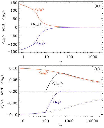
Figure 18: Similar to Fig. 11, but with parameters similar to Run VI (a) and Run P (b), where $\eta_{\rm ACC}\approx 13$ is much less than $\eta_{\rm flip}$ and $\eta_{\rm ACC}\approx 5\times 10^{4}$ is much greater than $\eta_{\rm flip}$. As for Run F in Fig. 11, we have $\eta_{\rm flip}=100$ also here for both runs, but do not consider finite values of $\eta_{\rm off}$.

Appendix C Behavior in imbalanced chirality decay

In Sect. V, we emphasized that even the slightest initial imbalance between magnetic helicity and fermion chirality will amplify as the magnetic energy decays. It is therefore important to remember that the dynamics discussed in this paper is specific to the case of balanced chirality, which is arguably also the most generic case. We know that the decay of magnetic energy and the increase of the correlation length follow a different behavior in the completely imbalanced case compared to the unbalanced one. We now discuss the behavior for the mildly imbalanced case. Here, we show that there is a tendency for the system to approach the behavior of a completely imbalanced one.

We discuss two runs, Run A where the initial $\langle\mu_{\rm M}\rangle$ is enhanced by 20% compared with $|\langle\mu_{5}\rangle|$, and Run B where it is decreased by 20%. Apart from that, the runs are the same as Run O, i.e., the run discussed in Ref. Brandenburg et al. (2023).

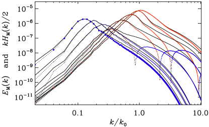
Figure 19: Magnetic energy (solid lines) and normalized helicity spectra $kH_{\rm M}(k)/2$ (dotted lines with red and blue symbols for positive and negative helicity spectra, respectively) for Run A at times $\eta=32$, 100, $320$, 1000, 3200, 15,000, 22,000, and 32,000.

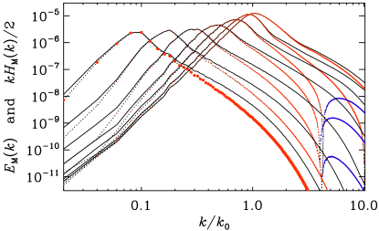
Figure 20: Same as Fig. 3, but for Run B at times $\eta=32$, 100, $320$, 1000, 3200, 10,000, and 32,000.

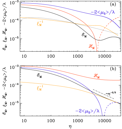
Figure 21: Time dependence of ${\cal E}_{\rm M}$ (black), $\xi_{\rm M}^{-1}$ (orange), ${\cal H}_{\rm M}$ (red), and $-2\langle\mu_{5}\rangle/\lambda$ (blue), for (a) Run A with smaller and (b) Run B with larger magnetic helicity than in the balanced case. Dashed lines indicate negative values; at late times $-2\langle\mu_{5}\rangle/\lambda$ changes sign in (a), and ${\cal H}_{\rm M}$ changes sign in (b). In (a) the dotted line denotes the $\eta^{-1/2}\log(\eta/\eta_{\log})$ scaling of Ref. Schober et al. (2020) with $\eta_{\log}=3$.

In Run A, where the magnetic helicity is weaker than in Run O, the CPI becomes dominant and overcompensates the magnetic helicity. The net chirality is then negative. Eventually, the sign of the magnetic helicity changes and all the remaining fermion chirality is converted to magnetic fields with negative helicity; see Fig. 19, where we show the magnetic energy ${\cal E}_{\rm M}(k,t)$ and the normalized magnetic helicity spectra $kH_{\rm M}(k)/2$ for Run A at times $\eta=32$, $320$, 1000, 3200, 10,000, and 32,000. We see that $k|H_{\rm M}(k)|/2$ approaches ${\cal E}_{\rm M}(k)$ near the maximum. In view of the spectral realizability condition, Eq. (16), this means that the magnetic field is fully helical. Away from the maxima, the inequality is no longer saturated, but this is a typical effect in all turbulent flows where the current helicity spectrum shows a Kolmogorov-type spectrum, making the magnetic helicity spectrum therefore steeper than what could still be allowed by the spectral realizability condition Brandenburg and Subramanian (2005).

On the other hand, when the fermion chirality is weak (Run B), the usual inverse magnetic cascade quickly gets established; see Fig. 20. In either case, the fermion chirality gets ultimately converted into magnetic helicity. It just takes a little longer than when the magnetic helicity is initially weak. At the end, however, the usual inverse cascade for a fully helical magnetic field commences. The sign of magnetic helicity can be positive or negative, depending on the sign of the initial total chirality.

To illustrate how the decay laws change when magnetic helicity and fermion chirality no longer balance, we plot in Fig. 21 the time dependencies of ${\cal E}_{\rm M}$, $\xi_{\rm M}$, ${\cal H}_{\rm M}$, and $-2\langle\mu_{5}\rangle/\lambda$, for (a) Run A with 20% smaller and (b) Run B with 20% larger magnetic helicity than in the balanced case. In both cases, we see a tendency of the decays of ${\cal E}_{\rm M}$ and $\xi_{\rm M}^{-1}$ to slow down while those of ${\cal H}_{\rm M}$ and $-2\langle\mu_{5}\rangle/\lambda$ follow separate evolutions. Especially in the case of Run B, where the magnetic helicity dominates of the fermion chirality, we see a tendency toward a ${\cal E}_{\rm M}\propto\xi^{-1}\propto t^{-2/3}$ as well as $\mathcal{H}_{\mathrm{M}}={\rm const}{}$ evolution, as expected from magnetic helicity conservation.

References

- Son and Surowka (2009) D. T. Son and P. Surowka, Phys. Rev. Lett. 103, 191601 (2009), arXiv:0906.5044 [hep-th] .
- Neiman and Oz (2011) Y. Neiman and Y. Oz, J. High. Energy Phys. 03, 023 (2011), arXiv:1011.5107 [hep-th] .
- Boyarsky et al. (2012) A. Boyarsky, J. Fröhlich, and O. Ruchayskiy, Phys. Rev. Lett. 108, 031301 (2012), arXiv:1109.3350 [astro-ph.CO] .
- Boyarsky et al. (2015) A. Boyarsky, J. Fröhlich, and O. Ruchayskiy, Phys. Rev. D 92, 043004 (2015), arXiv:1504.04854 [hep-ph] .
- Pavlović et al. (2017) P. Pavlović, N. Leite, and G. Sigl, Phys. Rev. D 96, 023504 (2017), arXiv:1612.07382 [astro-ph.CO] .
- Rogachevskii et al. (2017) I. Rogachevskii, O. Ruchayskiy, A. Boyarsky, J. Fröhlich, N. Kleeorin, A. Brandenburg, and J. Schober, Astrophys. J. 846, 153 (2017), arXiv:1705.00378 [physics.plasm-ph] .
- Brandenburg et al. (2017) A. Brandenburg, J. Schober, I. Rogachevskii, T. Kahniashvili, A. Boyarsky, J. Fröhlich, O. Ruchayskiy, and N. Kleeorin, Astrophys. J. 845, L21 (2017).
- Schober et al. (2018) J. Schober, I. Rogachevskii, A. Brandenburg, A. Boyarsky, J. Fröhlich, O. Ruchayskiy, and N. Kleeorin, Astrophys. J. 858, 124 (2018).
- Del Zanna and Bucciantini (2018) L. Del Zanna and N. Bucciantini, Mon. Not. R. Astron. Soc. 479, 657 (2018), arXiv:1806.07114 [astro-ph.HE] .
- Adler (1969) S. L. Adler, Phys. Rev. 177, 2426 (1969).
- Bell and Jackiw (1969) J. S. Bell and R. Jackiw, Nuovo Cim. A 60, 47 (1969).
- Joyce and Shaposhnikov (1997) M. Joyce and M. Shaposhnikov, Phys. Rev. Lett. 79, 1193 (1997).
- Akamatsu and Yamamoto (2013) Y. Akamatsu and N. Yamamoto, Phys. Rev. Lett. 111, 052002 (2013), arXiv:1302.2125 [nucl-th] .
- Hirono et al. (2015) Y. Hirono, D. E. Kharzeev, and Y. Yin, Phys. Rev. D 92, 125031 (2015), arXiv:1509.07790 [hep-th] .
- Schober et al. (2020) J. Schober, T. Fujita, and R. Durrer, Phys. Rev. D 101, 103028 (2020), arXiv:2002.09501 [physics.plasm-ph] .
- Manuel and Torres-Rincon (2015) C. Manuel and J. M. Torres-Rincon, Phys. Rev. D 92, 074018 (2015), arXiv:1501.07608 [hep-ph] .
- Domcke et al. (2019a) V. Domcke, Y. Ema, K. Mukaida, and R. Sato, J. High Energy Phys. 2019, 111 (2019a), arXiv:1812.08021 [hep-ph] .
- Domcke et al. (2020) V. Domcke, Y. Ema, and K. Mukaida, J. High. Energy Phys. 2020, 55 (2020), arXiv:1910.01205 [hep-ph] .
- Giovannini and Shaposhnikov (1998a) M. Giovannini and M. E. Shaposhnikov, Phys. Rev. D 57, 2186 (1998a), arXiv:hep-ph/9710234 .
- Giovannini and Shaposhnikov (1998b) M. Giovannini and M. E. Shaposhnikov, Phys. Rev. Lett. 80, 22 (1998b), arXiv:hep-ph/9708303 .
- Dvornikov and Semikoz (2012) M. Dvornikov and V. B. Semikoz, J. Cosmol. Astropart. Phys. 02, 040 (2012), [Erratum: J. Cosmol. Astropart. Phys.,08, E01 (2012)], arXiv:1111.6876 [hep-ph] .
- Tashiro et al. (2012) H. Tashiro, T. Vachaspati, and A. Vilenkin, Phys. Rev. D 86, 105033 (2012), arXiv:1206.5549 [astro-ph.CO] .
- Long et al. (2014) A. J. Long, E. Sabancilar, and T. Vachaspati, J. Cosmol. Astropart. Phys. 02, 036 (2014), arXiv:1309.2315 [astro-ph.CO] .
- Fujita and Kamada (2016) T. Fujita and K. Kamada, Phys. Rev. D 93, 083520 (2016), arXiv:1602.02109 [hep-ph] .
- Kamada and Long (2016a) K. Kamada and A. J. Long, Phys. Rev. D 94, 063501 (2016a), arXiv:1606.08891 [astro-ph.CO] .
- Kamada and Long (2016b) K. Kamada and A. J. Long, Phys. Rev. D 94, 123509 (2016b), arXiv:1610.03074 [hep-ph] .
- Pavlović et al. (2017) P. Pavlović, N. Leite, and G. Sigl, Phys. Rev. D 96, 023504 (2017), arXiv:1612.07382 [astro-ph.CO] .
- Schober et al. (2022a) J. Schober, I. Rogachevskii, and A. Brandenburg, Phys. Rev. Lett. 128, 065002 (2022a), arXiv:2107.12945 [physics.plasm-ph] .
- Schober et al. (2022b) J. Schober, I. Rogachevskii, and A. Brandenburg, Phys. Rev. D 105, 043507 (2022b), arXiv:2107.13028 [physics.plasm-ph] .
- García-Bellido et al. (1999) J. García-Bellido, D. Grigoriev, A. Kusenko, and M. Shaposhnikov, Phys. Rev. D 60, 123504 (1999), arXiv:hep-ph/9902449 [hep-ph] .
- Kamada (2018) K. Kamada, Phys. Rev. D 97, 103506 (2018), arXiv:1802.03055 [hep-ph] .
- Domcke et al. (2021) V. Domcke, K. Kamada, K. Mukaida, K. Schmitz, and M. Yamada, Phys. Rev. Lett. 126, 201802 (2021), arXiv:2011.09347 [hep-ph] .
- Yoshimura (1978) M. Yoshimura, Phys. Rev. Lett. 41, 281 (1978), [Erratum: ibid. 42, 746 (1979)].
- Dimopoulos and Susskind (1978) S. Dimopoulos and L. Susskind, Phys. Rev. D 18, 4500 (1978).
- Toussaint et al. (1979) D. Toussaint, S. Treiman, F. Wilczek, and A. Zee, Phys. Rev. D 19, 1036 (1979).
- Weinberg (1979) S. Weinberg, Phys. Rev. Lett. 42, 850 (1979).
- Barr et al. (1979) S. M. Barr, G. Segre, and H. Weldon, Phys. Rev. D 20, 2494 (1979).
- Ohnishi and Yamamoto (2014) A. Ohnishi and N. Yamamoto, (2014), arXiv:1402.4760 [astro-ph.HE] .
- Grabowska et al. (2015) D. Grabowska, D. B. Kaplan, and S. Reddy, Phys. Rev. D 91, 085035 (2015), arXiv:1409.3602 [hep-ph] .
- Masada et al. (2018) Y. Masada, K. Kotake, T. Takiwaki, and N. Yamamoto, Phys. Rev. D 98, 083018 (2018), arXiv:1805.10419 [astro-ph.HE] .
- Dvornikov et al. (2020) M. Dvornikov, V. B. Semikoz, and D. D. Sokoloff, Phys. Rev. D 101, 083009 (2020), arXiv:2001.08139 [astro-ph.HE] .
- Matsumoto et al. (2022) J. Matsumoto, N. Yamamoto, and D.-L. Yang, Phys. Rev. D 105, 123029 (2022), arXiv:2202.09205 [astro-ph.HE] .
- Kamada et al. (2023) K. Kamada, N. Yamamoto, and D.-L. Yang, Prog. Part. Nucl. Phys. 129, 104016 (2023), arXiv:2207.09184 [astro-ph.CO] .
- Domcke and Mukaida (2018) V. Domcke and K. Mukaida, J. Cosmol. Astropart. Phys. 2018, 020 (2018).
- Campbell et al. (1992) B. A. Campbell, S. Davidson, J. R. Ellis, and K. A. Olive, Phys. Lett. B 297, 118 (1992), arXiv:hep-ph/9302221 .
- Bödeker and Schröder (2019) D. Bödeker and D. Schröder, J. Cosmol. Astropart. Phys. 05, 010 (2019), arXiv:1902.07220 [hep-ph] .
- Jiménez et al. (2017) D. Jiménez, K. Kamada, K. Schmitz, and X.-J. Xu, J. Cosmol. Astropart. Phys. 12, 011 (2017), arXiv:1707.07943 [hep-ph] .
- Domcke et al. (2019b) V. Domcke, B. von Harling, E. Morgante, and K. Mukaida, J. Cosmol. Astropart. Phys. 2019, 032 (2019b), arXiv:1905.13318 [hep-ph] .
- Domcke et al. (2023) V. Domcke, K. Kamada, K. Mukaida, K. Schmitz, and M. Yamada, J. High. Energy Phys. 01, 053 (2023), arXiv:2210.06412 [hep-ph] .
- Kamada et al. (2021) K. Kamada, F. Uchida, and J. Yokoyama, J. Cosmol. Astropart. Phys. 04, 034 (2021), arXiv:2012.14435 [astro-ph.CO] .
- Hatori (1984) T. Hatori, J. Phys. Soc. Jpn. 53, 2539 (1984).
- Biskamp and Müller (1999) D. Biskamp and W.-C. Müller, Phys. Rev. Lett. 83, 2195 (1999), arXiv:physics/9903028 [physics.flu-dyn] .
- Kahniashvili et al. (2013) T. Kahniashvili, A. G. Tevzadze, A. Brandenburg, and A. Neronov, Phys. Rev. D 87, 083007 (2013), arXiv:1212.0596 [astro-ph.CO] .
- Brandenburg and Kahniashvili (2017) A. Brandenburg and T. Kahniashvili, Phys. Rev. Lett. 118, 055102 (2017), arXiv:1607.01360 [physics.flu-dyn] .
- Brandenburg et al. (2023) A. Brandenburg, K. Kamada, and J. Schober, Phys. Rev. Research 5, L022028 (2023), arXiv:2302.00512 [physics.plasm-ph] .
- Hosking and Schekochihin (2021) D. N. Hosking and A. A. Schekochihin, Phys. Rev. X 11, 041005 (2021), arXiv:2012.01393 [physics.flu-dyn] .
- Hosking and Schekochihin (2022) D. N. Hosking and A. A. Schekochihin, (2022), arXiv:2203.03573 [astro-ph.CO] .
- Zhou et al. (2022) H. Zhou, R. Sharma, and A. Brandenburg, J. Plasma Phys. 88, 905880602 (2022), arXiv:2206.07513 [physics.plasm-ph] .
- Brandenburg and Larsson (2023) A. Brandenburg and G. Larsson, Atmosphere 14, 932 (2023), arXiv:2305.08769 [physics.plasm-ph] .
- Brandenburg (2023) A. Brandenburg, J. Plasma Phys. 89, 175890101 (2023), arXiv:2211.14197 [physics.plasm-ph] .
- Goldreich and Reisenegger (1992) P. Goldreich and A. Reisenegger, Astrophys. J. 395, 250 (1992).
- Vilenkin (1980) A. Vilenkin, Phys. Rev. D 22, 3080 (1980).
- Alekseev et al. (1998) A. Yu. Alekseev, V. V. Cheianov, and J. Fröhlich, Phys. Rev. Lett. 81, 3503 (1998), arXiv:cond-mat/9803346 [cond-mat] .
- Fukushima et al. (2008) K. Fukushima, D. E. Kharzeev, and H. J. Warringa, Phys. Rev. D78, 074033 (2008), arXiv:0808.3382 [hep-ph] .
- Brandenburg et al. (1996) A. Brandenburg, K. Enqvist, and P. Olesen, Phys. Rev. D 54, 1291 (1996), arXiv:astro-ph/9602031 [astro-ph] .
- Brandenburg et al. (2021) A. Brandenburg, Y. He, T. Kahniashvili, M. Rheinhardt, and J. Schober, Astrophys. J. 911, 110 (2021), arXiv:2101.08178 [astro-ph.CO] .
- Pencil Code Collaboration et al. (2021) Pencil Code Collaboration, A. Brandenburg, A. Johansen, P. Bourdin, W. Dobler, W. Lyra, M. Rheinhardt, S. Bingert, N. Haugen, A. Mee, F. Gent, N. Babkovskaia, C.-C. Yang, T. Heinemann, B. Dintrans, D. Mitra, S. Candelaresi, J. Warnecke, P. Käpylä, A. Schreiber, P. Chatterjee, M. Käpylä, X.-Y. Li, J. Krüger, J. Aarnes, G. Sarson, J. Oishi, J. Schober, R. Plasson, C. Sandin, E. Karchniwy, L. Rodrigues, A. Hubbard, G. Guerrero, A. Snodin, I. Losada, J. Pekkilä, and C. Qian, J. Open Source Softw. 6, 2807 (2021).
- Rempel (2014) M. Rempel, Astrophys. J. 789, 132 (2014), arXiv:1405.6814 [astro-ph.SR] .
- (69) See Fig. 7 of the Pencil Code Newsletter 2022/2; https://github.com/pencil-code/website.
- Moffatt (1978) H. K. Moffatt, Magnetic field generation in electrically conducting fluids (1978).
- Durrer and Caprini (2003) R. Durrer and C. Caprini, J. Cosmol. Astropart. Phys. 2003, 010 (2003), arXiv:astro-ph/0305059 [astro-ph] .
- Baym and Heiselberg (1997) G. Baym and H. Heiselberg, Phys. Rev. D 56, 5254 (1997), arXiv:astro-ph/9704214 .
- Arnold et al. (2000) P. B. Arnold, G. D. Moore, and L. G. Yaffe, J. High. Energy Phys. 11, 001 (2000), arXiv:hep-ph/0010177 .
- Brandenburg et al. (2015) A. Brandenburg, T. Kahniashvili, and A. G. Tevzadze, PhRvL 114, 075001 (2015), arXiv:1404.2238 .
- Aghanim et al. (2020) N. Aghanim et al. (Planck), Astron. Astrophys. 641, A6 (2020), [Erratum: Astron.Astrophys. 652, C4 (2021)], arXiv:1807.06209 [astro-ph.CO] .
- Workman et al. (2022) R. L. Workman et al. (Particle Data Group), Prog. Theor. Exp. Phys. 2022, 083C01 (2022).
- (77) A. Brandenburg, K. Kamada, K. Mukaida, K. Schmitz, and J. Schober, Datasets for Chiral Magnetohydrodynamics with Zero Total Chirality, doi:10.5281/zenodo.8267336 (v2023.08.20); see also http://norlx65.nordita.org/~brandenb/proj/0Chir/ for easier access 10.5281/zenodo.8267336.
- Brandenburg and Subramanian (2005) A. Brandenburg and K. Subramanian, Astron. Astrophys. 439, 835 (2005), astro-ph/0504222 .