New Developments in Relativistic Viscous Hydrodynamics

Abstract

Starting with a brief introduction into the basics of relativistic fluid dynamics, I discuss our current knowledge of a relativistic theory of fluid dynamics in the presence of (mostly shear) viscosity. Derivations based on the generalized second law of thermodynamics, kinetic theory, and a complete second-order gradient expansion are reviewed. The resulting fluid dynamic equations are shown to be consistent for all these derivations, when properly accounting for the respective region of applicability, and can be applied to both weakly and strongly coupled systems. In its modern formulation, relativistic viscous hydrodynamics can directly be solved numerically. This has been useful for the problem of ultrarelativistic heavy-ion collisions, and I will review the setup and results of a hydrodynamic description of experimental data for this case.

I Introduction

I.1 Non-relativistic fluid dynamics

Fluid dynamics is one of the oldest and most successful theories in modern physics. In its non-relativistic form, it is intuitively understandable due to our everyday experience with hydrodynamics, or the dynamics of water. The degrees of freedom for an ideal, neutral, uncharged, one-component fluid are the fluid velocity ${\vec{v}}(t,{\vec{x}})$, the pressure $p(t,{\vec{x}})$, and the fluid mass density $\rho(t,{\vec{x}})$, which are linked by the fluid dynamic equations Euler ,LL §2,

$$\partial_{t}{\vec{v}}+\left({\vec{v}}\cdot{\vec{\partial}}\right){\vec{v}} = -\frac{1}{\rho}{\vec{\partial}}p\,,$$ (1)

$$\partial_{t}\rho+\rho\,{\vec{\partial}}\cdot{\vec{v}}+{\vec{v}}\cdot{\vec{\partial}}\rho = 0\ .$$ (2)

These equations are referred to as “Euler equation” (1) and “Continuity equation” (2), respectively, and typically have to be supplemented by an equation of state $p=p(\rho)$ to close the system. For non-ideal fluids, where dissipation can occur, the Euler equation generalizes to the “Navier-Stokes equation” Navier ; Stokes ,LL §15,

$$\frac{\partial v^{i}}{\partial t}+v^{k}\frac{\partial v^{i}}{\partial x^{k}} = -\frac{1}{\rho}\frac{\partial p}{\partial x^{i}}-\frac{1}{\rho}\frac{\partial\Pi^{ki}}{\partial x^{k}}\,,$$ (3)

$$\Pi^{ki} = -\eta\left(\frac{\partial v^{i}}{\partial x^{k}}+\frac{\partial v^{k}}{\partial x^{i}}-\frac{2}{3}\delta^{ki}\frac{\partial v^{l}}{\partial x^{l}}\right)-\zeta\,\delta^{ik}\frac{\partial v^{l}}{\partial x^{l}}\ ,$$ (4)

where Latin indices denote the three space directions, e.g. $i=1,2,3$. The viscous stress tensor $\Pi^{ki}$ contains the coefficients for shear viscosity, $\eta$, and bulk viscosity, $\zeta$, which are independent of velocity. The non-relativistic Navier-Stokes equation is well tested and found to be reliable in many applications, so any successful theory of relativistic viscous hydrodynamics should reduce to it in the appropriate limit.

I.2 Relativistic ideal fluid dynamics

For a relativistic system, the mass density $\rho(t,{\vec{x}})$ is not a good degree of freedom because it does not account for kinetic energy that may become sizable for motions close to the speed of light. Instead, it is useful to replace it by the total energy density $\epsilon(t,{\vec{x}})$, which reduces to $\rho$ in the non-relativistic limit. Similarly, $\vec{v}(t,{\vec{x}})$ is not a good degree of freedom because it does not transform appropriately under Lorentz transforms. Therefore, it should be replaced by the Lorentz 4-vector for the velocity,

$$u^{\mu}\equiv\frac{dx^{\mu}}{d{\cal T}},$$ (5)

where Greek indices denote Minkowski 4-space, e.g. $\mu=0,1,2,3$ with metric $g_{\mu\nu}={\rm diag}(+,-,-,-)$ (the same symbol for the metric will also be used for curved spacetimes). The proper time increment $d{\cal T}$ is given by the line element,

$$(d{\cal T})^{2} = g_{\mu\nu}dx^{\mu}dx^{\nu}=(dt)^{2}-(d{\vec{x}})^{2}\,,$$

$$= (dt)^{2}\left[1-\left(\frac{d\vec{x}}{dt}\right)^{2}\right]=(dt)^{2}\left[1-(\vec{v})^{2}\right]\ ,$$

where here and in the following, natural units $\hbar=c=k_{B}=1$ will be used. This implies that

$$u^{\mu}=\frac{dt}{d{\cal T}}\frac{dx^{\mu}}{dt}=\frac{1}{\sqrt{1-{\vec{v}}^{\,2}}}\left(\begin{array}[]{c}1\\ {\vec{v}}\end{array}\right)=\gamma(\vec{v})\left(\begin{array}[]{c}1\\ {\vec{v}}\end{array}\right)\ ,$$ (6)

which reduces to $u^{\mu}=(1,{\vec{v}})$ in the non-relativistic limit. In particular, one has $u^{\mu}=(1,{\vec{0}})$ if the fluid is locally at rest (“local rest frame”). Note that the 4-vector $u^{\mu}$ only contains three independent components since it obeys the relation

$$u^{2}\equiv u^{\mu}g_{\mu\nu}u^{\nu}=\gamma^{2}(\vec{v})\left(1-{\vec{v}}^{\,2}\right)=1,$$ (7)

so one does not need additional equations when trading ${\vec{v}}$ for the fluid 4-velocity $u^{\mu}$.

To obtain the relativistic fluid dynamic equations, it is sufficient to derive the energy-momentum tensor $T^{\mu\nu}$ for a relativistic fluid, as will be shown below. The energy-momentum tensor of an ideal relativistic fluid (denoted as $T^{\mu\nu}_{(0)}$) has to be built out of the hydrodynamic degrees of freedom, namely two Lorentz scalars ($\epsilon,p$) and one vector $u^{\mu}$, as well as the metric tensor $g_{\mu\nu}$. Since $T^{\mu\nu}$ should be symmetric and transform as a tensor under Lorentz transformations, the most general form allowed by symmetry is therefore

$$T^{\mu\nu}_{(0)}=\epsilon\left(c_{0}g^{\mu\nu}+c_{1}u^{\mu}u^{\nu}\right)+p\left(c_{2}g^{\mu\nu}+c_{3}u^{\mu}u^{\nu}\right)\ .$$ (8)

In the local restframe, one requires the $T_{(0)}^{00}$ component to represent the energy density $\epsilon$ of the fluid. Similarly, in the local rest frame, the momentum density should be vanishing $T_{(0)}^{0i}=0$, and the space-like components should be proportional to the pressure, $T_{(0)}^{ij}=p\,\delta^{ij}$ LL §133. Imposing these conditions onto the general form (8) leads to the equations

$$(c_{0}+c_{1})\epsilon+(c_{2}+c_{3})p=\epsilon,\qquad-c_{0}\epsilon-c_{2}p=p,$$ (9)

which imply $c_{0}=0,c_{1}=1,c_{2}=-1,c_{3}=1$, or $T^{\mu\nu}_{(0)}=\epsilon\,u^{\mu}u^{\nu}-p\,\left(g^{\mu\nu}-u^{\mu}u^{\nu}\right)$. For later convenience, it is useful to introduce the tensor

$$\Delta^{\mu\nu}=g^{\mu\nu}-u^{\mu}u^{\nu}.$$ (10)

It has the properties $\Delta^{\mu\nu}u_{\mu}=\Delta^{\mu\nu}u_{\nu}=0$ and $\Delta^{\mu\nu}\Delta_{\nu}^{\alpha}=\Delta^{\mu\alpha}$ and serves as a projection operator on the space orthogonal to the fluid velocity $u^{\mu}$. In this notation, the energy-momentum tensor of an ideal relativistic fluid becomes

$$T^{\mu\nu}_{(0)}=\epsilon\ u^{\mu}u^{\nu}-p\ \Delta^{\mu\nu}.$$ (11)

If there are no external sources, the energy-momentum tensor is conserved,

$$\partial_{\mu}T^{\mu\nu}_{(0)}=0\ .$$ (12)

It is useful project these equations in the direction parallel ($u_{\nu}\partial_{\mu}T^{\mu\nu}_{(0)}$) and perpendicular ($\Delta^{\alpha}_{\nu}\partial_{\mu}T^{\mu\nu}_{(0)}$) to the fluid velocity. For the first projection, one finds

$$u_{\nu}\partial_{\mu}T^{\mu\nu}_{(0)} = u^{\mu}\partial_{\mu}\epsilon+\epsilon\,(\partial_{\mu}u^{\mu})+\epsilon\,u_{\nu}u^{\mu}\partial_{\mu}u^{\nu}-p\,u_{\nu}\partial_{\mu}\Delta^{\mu\nu}\,,$$ (13)

$$=(\epsilon+p)\partial_{\mu}u^{\mu}+u^{\mu}\partial_{\mu}\epsilon=0\ ,$$

where the identity $u_{\nu}\partial_{\mu}u^{\nu}=\frac{1}{2}\partial_{\mu}(u_{\nu}u^{\nu})=\frac{1}{2}\partial_{\mu}1=0$ was used. For the other projection one finds

$$\Delta^{\alpha}_{\nu}\partial_{\mu}T^{\mu\nu}_{(0)} = \epsilon\,u^{\mu}\Delta^{\alpha}_{\nu}\partial_{\mu}u^{\nu}-\Delta^{\mu\alpha}(\partial_{\mu}p)+p\,u^{\mu}\Delta^{\alpha}_{\nu}\partial_{\mu}u^{\nu}\,,$$ (14)

$$= (\epsilon+p)\,u^{\mu}\partial_{\mu}u^{\alpha}-\Delta^{\mu\alpha}\partial_{\mu}p=0\ .$$

Introducing the shorthand notations

$$D\equiv u^{\mu}\partial_{\mu},\qquad\nabla^{\alpha}=\Delta^{\mu\alpha}\partial_{\mu}$$ (15)

for the projection of derivatives parallel and perpendicular to $u^{\mu}$, equations (13),(14) can be written as

$$D\epsilon+(\epsilon+p)\partial_{\mu}u^{\mu} = 0$$ (16)

$$(\epsilon+p)Du^{\alpha}-\nabla^{\alpha}p = 0\ .$$ (17)

These are the fundamental equations for a relativistic ideal fluid. Their meaning becomes transparent in the non-relativistic limit: for small velocities $|{\vec{v}}|\ll 1$ one finds

$$D=u^{\mu}\partial_{\mu}\simeq\partial_{t}+\vec{v}\cdot\vec{\partial}+{\cal O}(|\vec{v}|^{2}),\qquad\nabla^{i}=\Delta^{i\mu}\partial_{\mu}\simeq\partial^{i}+{\cal O}(|\vec{v}|),$$ (18)

so $D$ and $\nabla^{i}$ essentially reduce to time and space derivatives, respectively. Imposing further a non-relativistic equation of state where $p\ll\epsilon$, and that energy density is dominated by mass density $\epsilon\simeq\rho$, Eq. (16) becomes the continuity equation (2), and Eq. (17) the non-relativistic Euler equation (1).

One thus recognizes the fluid dynamic equations (both relativistic and non-relativistic) to be identical to the conservation equations for the fluid’s energy-momentum tensor.

II Relativistic Viscous Hydrodynamics

II.1 The relativistic Navier-Stokes equation

In the ideal fluid picture, all dissipative (viscous) effects are by definition neglected. If one is interested in a fluid description that includes for instance the effects of viscosity, one has to go beyond the ideal fluid limit, and in particular the fluid’s energy momentum tensor will no longer have the form Eq. (11). Instead, one writes

$$T^{\mu\nu}=T^{\mu\nu}_{(0)}+\Pi^{\mu\nu},$$ (19)

where $T^{\mu\nu}_{(0)}$ is the familiar ideal fluid part given by Eq. (11) and $\Pi^{\mu\nu}$ is the viscous stress tensor that includes the contributions to $T^{\mu\nu}$ stemming from dissipation. Considering for simplicity a system without conserved charges (or at zero chemical potential), all momentum density is due to the flow of energy density

$$u_{\mu}T^{\mu\nu}=\epsilon\,u^{\nu}\longrightarrow\quad u_{\mu}\Pi^{\mu\nu}=0.$$ (20)

While here this is the only possibility, for a more general system with conserved charges one can view this as a choice of frame for the definition of the fluid 4-velocity, sometimes referred to as Landau-Lifshitz frame. This can be easily understood by recognizing that in a system with a conserved charge there will be an associated charge current $n^{\mu}$ that can be used alternatively to define the fluid velocity, e.g. the Eckart frame $u_{\mu}n^{\mu}=n$. These choices reflect the freedom of defining the local rest frame either as the frame where the energy density (Landau-Lifshitz) or the charge density (Eckart) is at rest. Since the physics must be the same in either of these frames, one can show that charge diffusion in one frame is related to heat flow in the other frame, as done e.g. in the appendix of Son:2006em . For other recent discussions of relativistic viscous hydrodynamics in the presence of conserved charges, see e.g. Rischke:1998fq ; Muronga:2003ta .

Similar to the case of ideal fluid dynamics studied in section I.2, the fundamental equations of viscous fluid dynamics are found by taking the appropriate projections of the conservation equations of the energy momentum tensor,

$$u_{\nu}\partial_{\mu}T^{\mu\nu} = D\epsilon+(\epsilon+p)\partial_{\mu}u^{\mu}+u_{\nu}\partial_{\mu}\Pi^{\mu\nu}=0\,,$$

$$\Delta_{\nu}^{\alpha}\partial_{\mu}T^{\mu\nu} = (\epsilon+p)Du^{\alpha}-\nabla^{\alpha}p+\Delta^{\alpha}_{\nu}\partial_{\mu}\Pi^{\mu\nu}=0\ .$$ (21)

The first equation can be further simplified by rewriting $u_{\nu}\partial_{\mu}\Pi^{\mu\nu}=\partial_{\mu}\left(u_{\nu}\Pi^{\mu\nu}\right)-\Pi^{\mu\nu}\partial_{(\mu}u_{\nu)}$, and using the identity

$$\partial_{\mu}=u_{\mu}D+\nabla_{\mu}$$ (22)

as well as the choice of frame, $u_{\mu}\Pi^{\mu\nu}=0$. Here and in the following the $(\ldots)$ denote symmetrization, e.g.

$$A_{(\mu}B_{\nu)}=\frac{1}{2}\left(A_{\mu}B_{\nu}+A_{\nu}B_{\mu}\right)\ .$$

Hence, the fundamental equations for relativistic viscous fluid dynamics are

$\displaystyle D\epsilon+(\epsilon+p)\partial_{\mu}u^{\mu}-\Pi^{\mu\nu}\nabla_{(\mu}u_{\nu)}$ $\displaystyle=$ $\displaystyle 0\,,$ $\displaystyle(\epsilon+p)Du^{\alpha}-\nabla^{\alpha}p+\Delta^{\alpha}_{\nu}\partial_{\mu}\Pi^{\mu\nu}$ $\displaystyle=$ $\displaystyle 0\ .$ (23)

At this point, however, the viscous stress tensor has not been specified. Indeed, much of the remainder of this work will deal with deriving expressions for $\Pi^{\mu\nu}$, which together with (23) will give different theories of viscous hydrodynamics.

An elegant way of obtaining $\Pi^{\mu\nu}$ builds upon the second law of thermodynamics, which states that entropy must always increase locally. The entropy density $s$ is connected to energy density, pressure and temperature $T$ by the basic equilibrium thermodynamic relations for a system without conserved charges (or zero chemical potential),

$$\epsilon+p=Ts,\qquad Tds=d\epsilon\ .$$ (24)

The second law of thermodynamics can be recast in the covariant form

$$\partial_{\mu}s^{\mu}\geq 0$$ (25)

using the entropy 4-current $s^{\mu}$ which in equilibrium is given by

$$s^{\mu}=su^{\mu}\ .$$ (26)

The thermodynamic relations (24) allow to rewrite the second law (25) as

$$\partial_{\mu}s^{\mu}=Ds+s\partial_{\mu}u^{\mu}=\frac{1}{T}D\epsilon+\frac{\epsilon+p}{T}\partial_{\mu}u^{\mu}=\frac{1}{T}\Pi^{\mu\nu}\nabla_{(\mu}u_{\nu)}\geq 0\ ,$$ (27)

where (23) was used to rewrite $D\epsilon$. It is customary to split $\Pi^{\mu\nu}$ into a part $\pi^{\mu\nu}$ that is traceless, $\pi^{\mu}_{\mu}=0$, and a remainder with non-vanishing trace,

$$\Pi^{\mu\nu}=\pi^{\mu\nu}+\Delta^{\mu\nu}\Pi\ .$$ (28)

Similarly one introduces a new notation for the traceless part of $\nabla_{(\mu}u_{\nu)}$,

$$\nabla_{<\mu}u_{\nu>}\equiv 2\nabla_{(\mu}u_{\nu)}-\frac{2}{3}\Delta_{\mu\nu}\nabla_{\alpha}u^{\alpha}\,,$$ (29)

so that the the second law becomes

$$\partial_{\mu}s^{\mu}=\frac{1}{2T}\pi^{\mu\nu}\nabla_{<\mu}u_{\nu>}+\frac{1}{T}\Pi\nabla_{\alpha}u^{\alpha}\geq 0\ .$$ (30)

One recognizes that this inequality is guaranteed to be fulfilled if

$$\pi^{\mu\nu}=\eta\nabla^{<\mu}u^{\nu>}\,,\quad\Pi=\zeta\nabla_{\alpha}u^{\alpha}\,,\quad\eta\geq 0\,,\quad\zeta\geq 0\,,$$ (31)

because then $\partial_{\mu}s^{\mu}$ is a positive sum of squares.

In the non-relativistic limit, the viscous stress tensor becomes that of the Navier-Stokes equations (4), which leads one to equate $\eta,\zeta$ with the shear and bulk viscosity coefficient, respectively. Also, for this reason we refer to the system of equations (23),(28),(31) as the relativistic Navier-Stokes equation. While beautifully simple, it turns out that the relativistic Navier-Stokes equation – unlike its non-relativistic counterpart – exhibits pathologies for all but the simplest flow profiles, as will be shown below.

II.2 Acausality problem of the relativistic Navier-Stokes equation

Let us consider small perturbations of the energy density and fluid velocity in a system that is initially in equilibrium and at rest,

$$\epsilon=\epsilon_{0}+\delta\epsilon(t,x),\qquad u^{\mu}=(1,{\vec{0}})+\delta u^{\mu}(t,x),$$ (32)

where for simplicity the perturbation was assumed to be dependent on one space coordinate only. The relativistic Navier-Stokes equation then specifies the space-time evolution of the perturbations. For the particular direction $\alpha=y$, Eq. (23) gives

$$(\epsilon+p)Du^{y}-\nabla^{y}p+\Delta^{y}_{\nu}\partial_{\mu}\Pi^{\mu\nu} = (\epsilon_{0}+p_{0})\partial_{t}\delta u^{y}+\partial_{x}\Pi^{xy}+{\cal O}(\delta^{2})\,,$$

$$\Pi^{xy}=\eta\left(\nabla^{x}u^{y}+\nabla^{y}u^{x}\right)+\left(\zeta-\frac{2}{3}\eta\right)\Delta^{xy}\nabla_{\alpha}u^{\alpha} = -\eta_{0}\ \partial_{x}\delta u^{y}+{\cal O}(\delta^{2})\ .$$

This implies a diffusion-type evolution equation for the perturbation $\delta u^{y}(t,x)$:

$$\partial_{t}\delta u^{y}-\frac{\eta_{0}}{\epsilon_{0}+p_{0}}\partial_{x}^{2}\delta u^{y}={\cal O}(\delta^{2})\ .$$ (33)

To investigate the individual modes of this diffusion process, one can insert a mixed Laplace-Fourier wave ansatz

$$\delta u^{y}(t,x)=e^{-\omega t+ikx}f_{\omega,k}$$

into Eq. (33). This gives the “dispersion-relation” of the diffusion equation,

$$\omega=\frac{\eta_{0}}{\epsilon_{0}+p_{0}}k^{2}\ ,$$ (34)

which one can use to estimate the speed of diffusion of a mode with wavenumber $k$,

$$v_{T}(k)=\frac{d\omega}{dk}=2\frac{\eta_{0}}{\epsilon_{0}+p_{0}}k\ .$$ (35)

One finds that $v_{T}$ is linearly dependent on the wavenumber, which implies that as $k$ becomes larger and larger, the diffusion speed will grow without bound. In particular, at some sufficiently large value of $k$, $v_{T}(k)$ will exceed the speed of light, which violates causality. Therefore the relativistic Navier-Stokes equation does not constitute a causal theory.

The obvious conclusion to draw from this argument is that the relativistic Navier-Stokes equation exhibits unphysical behavior for the short wavelength ($k\gg 1$) modes and hence can only be valid in the description of the long wavelength modes. This is not a principal problem, as one can regard hydrodynamics simply as an effective theory of matter in the long wavelength, $k\rightarrow 0$ limit. However, having a finite range of validity in $k$ typically is a practical problem when dealing with more complicated flow profiles that do not lend themselves to analytic solutions and have to be solved numerically. In this case, it turns out that the high $k$ modes are associated with instabilities Hiscock:1985zz that make it necessary to regulate the theory by other means. A simple argument to understand the practical problem can be given as follows: modes that travel faster than the speed of light in one Lorentz frame correspond to modes traveling backwards in time in a different frame. Hydrodynamics is an initial value problem which requires a well defined set of initial conditions. However, if there are modes present in the equations that travel backwards in time, the initial conditions cannot be given freely Kostadt:2000ty , and as a consequence one cannot solve the relativistic Navier-Stokes equation numerically.

One possible way to regulate the theory is provided by considering the “Maxwell-Cattaneo law” Maxwell ; Cattaneo

$$\tau_{\pi}\partial_{t}\Pi^{xy}+\Pi^{xy}=-\eta_{0}\partial_{x}\delta u^{y}\,$$ (36)

instead of the Navier-Stokes equation. Here $\tau_{\pi}$ is a new transport coefficient sometimes referred to as relaxation time. The effect of this modification becomes apparent when recalculating the dispersion relation for the perturbation $\delta u^{y}$ using Eq. (36). One finds

$$\omega=\frac{\eta_{0}}{\epsilon_{0}+p_{0}}\frac{k^{2}}{1-\omega\tau_{\pi}}\ ,$$ (37)

which coincides with the dispersion relation of the diffusion equation Eq. (34) in the hydrodynamic ($\omega,k\rightarrow 0$) limit. More interestingly, however, is that for large frequency $\omega\gg 1$ Eq. (37) does not describe diffusive behavior, but instead propagating waves with a propagation speed that is finite in the limit of $k\gg 1$,

$$v_{T}^{\rm max}\equiv\lim_{k\rightarrow\infty}\frac{d|\omega|}{d\ k}=\sqrt{\frac{\eta_{0}}{(\epsilon_{0}+p_{0})\tau_{\pi}}}\ ,$$ (38)

unless $\tau_{\pi}\rightarrow 0$. Interestingly, for all known fluids the limiting value $\sqrt{\frac{\eta_{0}}{(\epsilon_{0}+p_{0})\tau_{\pi}}}$ has been found to be smaller than one, so that the Maxwell-Cattaneo law seems to be an extension of the Navier-Stokes equation that preserve causality.

For heat flow, the corresponding Maxwell-Cattaneo law implies a dispersion relation equivalent to Eq. (37), and there the propagating waves can be associated with the phenomenon of second sound Jou88 §4, joseph89 , observed experimentally in solid helium Ackerman66 . It is not known to me whether propagating high frequency shear waves, as suggested by Eq. (37), have been found in experiments.

While the Maxwell-Cattaneo law seems to be a successful phenomenological extension of the Navier-Stokes equation, it is unsatisfactory that Eq. (36) does not follow from a first-principles framework, but is rather introduced “by hand”. It will turn out, however, that the Maxwell-Cattaneo law – while not derivable – does seem to correctly capture some important aspects of relativistic viscous hydrodynamic theory, for instance that terms of higher order in $k$ (higher order gradients) are needed to restore causality.

II.3 Müller-Israel-Stewart theory, entropy-wise

In section II.1, the Navier-Stokes equation was derived from the second law of thermodynamics $\partial_{\mu}s^{\mu}\geq 0$ by using the form of the entropy current in equilibrium, $s^{\mu}=su^{\mu}$. However, it is not guaranteed that the entropy current equals its equilibrium expression for a dissipative fluid that can be out of equilibrium. Specifically, it was suggested Mueller1 ; IS0a that out of equilibrium the entropy current can have contributions from the viscous stress tensor, which is sometimes referred to as “extended irreversible thermodynamics” Jou88 ; Jou99 . Assuming that the entropy current has to be algebraic in the hydrodynamic degrees of freedom and that deviations from equilibrium are not too large so that high order corrections can be neglected, the entropy current has to be of the form Mueller1 ; IS0a ; Muronga:2003ta

$$s^{\mu}=su^{\mu}-\frac{\beta_{0}}{2T}u^{\mu}\Pi^{2}-\frac{\beta_{2}}{2T}u^{\mu}\pi_{\alpha\beta}\pi^{\alpha\beta}+{\cal O}(\Pi^{3})\ ,$$ (39)

where $\beta_{0},\beta_{2}$ are coefficients that quantify the effect of these second-order modifications of the entropy current. Using again Eq. (23) to rewrite $\partial_{\mu}s^{\mu}$ as in section II.1 one finds

$$\partial_{\mu}s^{\mu} = \frac{\pi^{\alpha\beta}}{2T}\left(\nabla_{<\alpha}u_{\beta>}-\pi_{\alpha\beta}TD\left(\frac{\beta_{2}}{T}\right)-2\beta_{2}D\pi_{\alpha\beta}-\beta_{2}\pi_{\alpha\beta}\partial_{\mu}u^{\mu}\right)$$ (40)

$$+\frac{\Pi}{T}\left(\nabla_{\alpha}u^{\alpha}-\frac{1}{2}\Pi\ TD\left(\frac{\beta_{0}}{T}\right)-\beta_{0}D\Pi-\frac{1}{2}\beta_{0}\Pi\partial_{\mu}u^{\mu}\right)\geq 0\ .$$

The inequality is guaranteed to be fulfilled if

$$\pi_{\alpha\beta} = \eta\left(\nabla_{<\alpha}u_{\beta>}-\pi_{\alpha\beta}TD\left(\frac{\beta_{2}}{T}\right)-2\beta_{2}D\pi_{\alpha\beta}-\beta_{2}\pi_{\alpha\beta}\partial_{\mu}u^{\mu}\right)\ ,$$

$$\Pi = \zeta\left(\nabla_{\alpha}u^{\alpha}-\frac{1}{2}\Pi\ TD\left(\frac{\beta_{0}}{T}\right)-\beta_{0}D\Pi-\frac{1}{2}\beta_{0}\Pi\partial_{\mu}u^{\mu}\right)\ ,$$ (41)

with $\eta,\zeta$ the usual bulk and shear viscosity coefficients. Note that Eq. (41) coincides with the Navier-Stokes equation in the limit of $\beta_{0},\beta_{2}\rightarrow 0$. For non-vanishing $\beta_{0},\beta_{2}$, Eq. (41) contains time derivatives of $\pi_{\alpha\beta},\Pi$, which are similar (but not identical) to the Maxwell-Cattaneo law Eq. (36) if one identifies $\beta_{2}=\frac{\tau_{\pi}}{2\eta}$ (and similarly, $\beta_{0}=\frac{\tau_{\Pi}}{\zeta}$). The set of equations (23),(41) (and some variations thereof) are commonly referred to as “Müller-Israel-Stewart” theory and will be discussed more in section III.

Similar to section II.2, one can study the causality properties of the Müller-Israel-Stewart theory by considering small perturbations around equilibrium, Eq. (32). Keeping only perturbations to first order, Eq. (23) and Eq. (41) become

$$\partial_{t}\delta\epsilon+(\epsilon_{0}+p_{0})\partial_{x}\delta u^{x}=0,\quad(\epsilon_{0}+p_{0})\partial_{t}\delta u^{x}+\partial_{x}p+\partial_{\mu}\delta\Pi^{\mu x}=0,$$

$$(\epsilon_{0}+p_{0})\partial_{t}\delta u^{y}+\partial_{\mu}\delta\Pi^{\mu y}=0,\quad\delta\Pi^{\mu\nu}=\delta\pi^{\mu\nu}+g^{\mu\nu}\delta\Pi$$

$$\delta\pi^{xx}+\tau_{\pi}\partial_{t}\delta\pi^{xx}=-\frac{4}{3}\eta_{0}\partial_{x}\delta u^{x},\quad\delta\pi^{xy}+\tau_{\pi}\partial_{t}\delta\pi^{xy}=-\eta_{0}\partial_{x}\delta u^{y},$$

$$\delta\Pi+\tau_{\Pi}\partial_{t}\delta\Pi=\zeta_{0}\partial_{x}\delta u^{x}\,.$$ (42)

The equation of state $\epsilon=\epsilon(p)$ relates the pressure and energy density gradients, $\partial_{x}p=\frac{dp}{d\epsilon}\partial_{x}\epsilon$, and the condition $u_{\mu}\Pi^{\mu\nu}=0$ implies $\delta\Pi^{t\nu}={\cal O}(\delta^{2})$. Using a Fourier ansatz

$$\delta\epsilon=e^{i\omega t-ikx}\delta\epsilon_{\omega,k},\quad\delta u^{i}=e^{i\omega t-ikx}\delta u^{i}_{\omega,k},\quad\delta\pi^{\mu\nu}=e^{i\omega t-ikx}\delta\pi^{\mu\nu}_{\omega,k},\quad\delta\Pi=e^{i\omega t-ikx}\delta\Pi^{\mu\nu}_{\omega,k},$$

in Eq. (42) gives the system of equations

$$i\omega\ \delta\epsilon_{\omega,k}-ik(\epsilon_{0}+p_{0})\ \delta u^{x}_{\omega,k} = 0,$$ (43)

$$i\omega(\epsilon_{0}+p_{0})\ \delta u^{x}_{\omega,k}-ik\frac{dp}{d\epsilon}\ \delta\epsilon_{\omega,k}-ik\left(\frac{4}{3}\frac{ik\eta_{0}}{1+i\omega\tau_{\pi}}+\frac{ik\zeta_{0}}{1+i\omega\tau_{\Pi}}\right)\delta u^{x}_{\omega,k} = 0,$$ (44)

$$i\omega(\epsilon_{0}+p_{0})\ \delta u^{y}_{\omega,k}-ik\left(\frac{ik\eta_{0}}{1+i\omega\tau_{\pi}}\right)\delta u^{y}_{\omega,k} = 0\,.$$ (45)

Eq. (45) corresponds to result from the Maxwell-Cattaneo law for the transverse velocity perturbation $\delta u^{y}$, discussed in section II.2. The other two equations correspond to density perturbations and longitudinal fluid velocity displacements, commonly known as sound. The sound dispersion relation is given by

$$i\omega-i\frac{k^{2}}{\omega}\frac{dp}{d\epsilon}+k^{2}\left(\frac{4}{3}\frac{\eta_{0}}{\epsilon_{0}+p_{0}}\frac{1}{1+i\omega\tau_{\pi}}+\frac{\zeta_{0}}{\epsilon_{0}+p_{0}}\frac{1}{1+i\omega\tau_{\Pi}}\right)=0\,,$$ (46)

and in the hydrodynamic limit ($\omega,k\ll 1$) becomes

$$\omega = \pm kc_{s}+ik^{2}\left(\frac{2}{3}\frac{\eta_{0}}{\epsilon_{0}+p_{0}}+\frac{1}{2}\frac{\zeta_{0}}{\epsilon_{0}+p_{0}}\right)$$ (47)

$$\mp\frac{k^{3}}{2c_{s}}\left[\left(\frac{2}{3}\frac{\eta_{0}}{\epsilon_{0}+p_{0}}+\frac{1}{2}\frac{\zeta_{0}}{\epsilon_{0}+p_{0}}\right)^{2}-2c_{s}^{2}\left(\frac{2}{3}\frac{\eta_{0}}{\epsilon_{0}+p_{0}}\tau_{\pi}+\frac{1}{2}\frac{\zeta_{0}}{\epsilon_{0}+p_{0}}\tau_{\Pi}\right)\right]+{\cal O}(k^{4})\,.$$

The quantity

$$c_{s}\equiv\sqrt{\frac{d\ p}{d\ \epsilon}}$$ (48)

can be recognized to be the speed of sound when calculating the group velocity $\lim_{k\rightarrow 0}\frac{d\omega}{dk}$. For large wavenumbers and frequencies, Eq. (46) gives a limiting sound mode group velocity of

$$v_{L}^{\rm max}\equiv\lim_{k\rightarrow\infty}\frac{d\omega}{dk}=\sqrt{c_{s}^{2}+\frac{4}{3}\frac{\eta_{0}}{\tau_{\pi}(\epsilon_{0}+p_{0})}+\frac{\zeta_{0}}{\tau_{\Pi}(\epsilon_{0}+p_{0})}}\,,$$ (49)

which together with the result for the transverse mode Eq. (38) suggests that the Müller-Israel-Stewart theory – derived via an extended second law of thermodynamics – constitutes a relativistic theory of viscous hydrodynamics that obeys causality if the relaxation times $\tau_{\pi},\tau_{\Pi}$ are not too small. Note that the requirement $v_{L}^{\rm max}\leq 1$ from Eq. (49) is more restrictive than Eq. (38) concerning the allowed values of $c_{s}^{2},\eta,\zeta,\tau_{\pi},\tau_{\Pi}$.

However, many questions remain unanswerable within this formalism, e.g. how to obtain the value of $\tau_{\pi},\tau_{\Pi}$, or whether the assumption that the entropy current should be algebraic in the hydrodynamic degrees of freedom is valid (Refs. Loganayagam:2008is ; Bhattacharyya:2008xc ; Romatschke:2009kr seem to indicate the contrary). Therefore, it is necessary to have a different derivation of viscous hydrodynamics.

III Fluid Dynamics from Kinetic Theory

III.1 A very short introduction to kinetic theory

Kinetic theory treats the evolution of the one-particle distribution function $f(\vec{p},t,\vec{x})$, which can be associated with the number of on-shell particles per unit phase space,

$$f(\vec{p},t,\vec{x})\propto\frac{dN}{d^{3}p\,d^{3}x}\,.$$ (50)

If collisions between particles can be neglected, the evolution of $f$ follows from Liouville’s theorem,

$$\frac{df}{d{\cal T}}=0=\frac{dt}{d{\cal T}}\frac{\partial f}{\partial t}+\frac{d\vec{x}}{d{\cal T}}\cdot\frac{\partial f}{\partial\vec{x}}$$ (51)

Multiplying (51) by the mass $m$ of a particle and recognizing $m\frac{dt}{d{\cal T}}=m\gamma(\vec{v})=p^{0}$, $m\frac{d{\vec{x}}}{d{\cal T}}=m{\vec{v}}\gamma(\vec{v})=\vec{p}$ as the particle’s energy and momentum, respectively, Eq. (51) becomes

$$p^{\mu}\partial_{\mu}f=0\,,$$ (52)

where $p^{\mu}$ has to fulfill the on-shell condition $p^{\mu}p_{\mu}=m^{2}$.

Eventually, collisions between particles cannot be neglected, and hence Eq. (51) is no longer valid. Taking the effect of collisions into account changes the evolution equation LL10 §3 to

$$p^{\mu}\partial_{\mu}f=-{\cal C}[f],$$ (53)

where ${\cal C}[f]$ is the collision term that is a functional of $f$ and the precise form of which depends on the particle interactions. Eq. (53) is known as the “Boltzmann-equation” Boltzmann . For a system in global equilibrium $f$ is stationary, $f(\vec{p},t,\vec{x})=f_{(0)}(\vec{p})$ so that the Boltzmann equation gives

$$p^{\mu}\partial_{\mu}f_{(0)}=0=-{\cal C}[f_{(0)}],$$

which implies that the collision term vanishes in equilibrium. Note that this means that Eq. (52) holds for two very different regimes, namely firstly when one can ignore collisions (and the system is typically far from equilibrium) and secondly when the collisions are strong enough to keep the system in equilibrium. The first case is typically applicable if the timescale of the description is short enough so that the effect of particle collisions can be neglected. Ultimately, however, particle collisions will become important and drive the system towards equilibrium. It is this second case, or more generally the long time (small frequency, long wavelength) limit that corresponds to hydrodynamics (see also the discussion in section II.2).

Given the interpretation of $f$ in Eq. (50), the particle number density should be proportional to $\int d^{3}pf$, or the sum of $f$ over all momenta with weight unity. Summing instead with a weight of particle energy $\int d^{3}p\ p^{0}f$, one expects a result proportional to the product of number density and energy, or energy density, which is a part of the energy-momentum tensor. More rigorously, one can define the relation between the particle distribution function and the energy-momentum tensor RKT as

$$\int\frac{d^{4}p}{(2\pi)^{3}}p^{\mu}p^{\nu}\delta(p^{\mu}p_{\mu}-m^{2})2\theta(p^{0})f(p,x)\equiv T^{\mu\nu}\,,$$ (54)

where the l.h.s. again can be understood as a sum over momenta, with the $\delta$-function imposing the condition of only counting on-shell particles and the step-function to restrict the sum to positive energy states.

III.2 Ideal fluid dynamics from kinetic theory

In the following, I will limit myself to considering the ultrarelativistic limit where all particle masses can be neglected, $m\rightarrow 0$. From Eq. (54), this leads to $T^{\mu}_{\mu}=0$, or vanishing conformal anomaly. Interpreting (54) as the fluid’s energy-momentum tensor, this amounts to setting the bulk viscosity coefficient to zero, $\zeta=0$ (cf. Eq. (19,31) and the discussion in section IV.5).

Introducing for convenience the shorthand notation

$$\int d\chi\equiv\frac{d^{4}p}{(2\pi)^{3}}\delta(p^{\mu}p_{\mu})2\theta(p^{0}),$$ (55)

and taking the first moment of the Boltzmann equation, one finds

$$\int d\chi p^{\nu}p^{\mu}\partial_{\mu}f(p^{\mu},x^{\mu})=-\int d\chi p^{\nu}{\cal C}[f]=\partial_{\mu}\int d\chi p^{\nu}p^{\mu}f(p,x)=\partial_{\mu}T^{\mu\nu}\ .$$ (56)

For particle interactions that conserve energy and momentum, the integral over the collision term vanishes, $\int d\chi p^{\nu}{\cal C}[f]=0$. If $T^{\mu\nu}$ can be interpreted as a fluid’s energy-momentum tensor, then this implies that the first moment of the Boltzmann equation corresponds to the fundamental equations of fluid dynamics (23), since these follow from $\partial_{\mu}T^{\mu\nu}=0$.

The interpretation of the kinetic theory energy-momentum tensor in the fluid picture is most transparent in equilibrium, where $f(\vec{p},t,\vec{x})=f_{(0)}(\vec{p})$. Similar to the discussion in the introduction, $f_{(0)}(\vec{p})$ is not an optimal description for a relativistic system, since it is not manifestly invariant under Lorentz transformations. It is better to trade $f_{(0)}$ with a more convenient function,

$$f_{(0)}(\vec{p})\rightarrow f_{\rm eq}\left(\frac{p^{\mu}u_{\mu}}{T}\right),$$

where $u^{\mu}$ is a four vector that reduces to $u^{\mu}\rightarrow(1,\vec{0})$ in the restframe of the heat bath with temperature $T$. Eq. (54) can then be written as

$$T^{\mu\nu}_{(0)}=\int d\chi p^{\mu}p^{\nu}f_{\rm eq}\left(\frac{p^{\mu}u_{\mu}}{T}\right)=a_{20}u^{\mu}u^{\nu}+a_{21}\Delta^{\mu\nu},$$ (57)

where in hindsight it is more convenient to choose $u^{\mu}u^{\nu},\Delta^{\mu\nu}$ as a tensor basis then $u^{\mu}u^{\nu},g^{\mu\nu}$. The coefficients $a_{20},a_{21}$ are functions of the temperature only and are determined by contracting (57) with $u^{\mu}u^{\nu}$ and $\Delta^{\mu\nu}$, respectively,

$$a_{20}=\int d\chi(p^{\mu}u_{\mu})^{2}f_{\rm eq}\left(\frac{p^{\mu}u_{\mu}}{T}\right),\quad a_{21}=\frac{1}{3}\int d\chi\left(p^{\mu}p_{\mu}-(p^{\mu}u_{\mu})^{2}\right)f_{\rm eq}\left(\frac{p^{\mu}u_{\mu}}{T}\right)\,.$$ (58)

Identifying $u^{\mu}$ with the fluid four velocity, Eq. (57) corresponds to the ideal fluid energy-momentum tensor Eq. (11) with $\epsilon=a_{20},p=-a_{21}$, and the equation of state $\epsilon=3\ p$ (or speed of sound squared $c_{s}^{2}=\frac{1}{3}$) following from on-shell condition in the massless limit, $p^{\mu}p_{\mu}=0$.

To calculate $a_{20},a_{21}$, one has to specify the equilibrium distribution function $f_{\rm eq}$. A concrete example where the evaluation is straightforward is for a single species of particles that obey Boltzmann statistics, so that $f_{\rm eq}\left(\frac{p^{\mu}u_{\mu}}{T}\right)=\exp{\left[-\left(\frac{p^{\mu}u_{\mu}}{T}\right)\right]}$. In this case, $a_{20}$ is easily calculated by choosing the convenient frame $u^{\mu}=(1,\vec{0})$, so that

$$a_{20}=\int\frac{d^{4}p}{(2\pi)^{3}}(p^{0})^{2}\delta\left((p^{0})^{2}-\vec{p}^{\,2}\right)2\theta(p^{0})e^{-p^{0}/T}=\frac{1}{2\pi^{2}}\int_{0}^{\infty}dp\ p^{3}e^{-p/T}=\frac{3T^{4}}{\pi^{2}},$$

and $a_{21}=-\frac{1}{3}a_{20}=-\frac{T^{4}}{\pi^{2}}$. For a single species of particles obeying Bose-Einstein statistics, $f_{\rm eq}(x)=\left[e^{x}-1\right]^{-1}$, the result would be $a_{20}=\frac{3T^{4}\pi^{2}}{90}$. The relation between $a_{20}$ and $\epsilon$ can be used to re-express the temperature in terms of the energy density.

III.3 Out of equilibrium

From Eq. (57) it is evident that when the argument of the distribution function $f$ depends only on scalars and one Lorentz vector $u^{\mu}$, the form of the energy-momentum tensor for kinetic theory is the same as for ideal fluid dynamics. If the system is locally in equilibrium, $f_{\rm eq}$ is completely characterized by a vector-valued function that specifies the local rest frame of the heat bath, $u^{\mu}(x)$, and the local temperature (or energy density). Therefore, a system that is in perfect local equilibrium is described by ideal fluid dynamics. Departures from equilibrium result in departures from the ideal fluid dynamics picture, and hence can only be captured with dissipative (viscous) fluid dynamics. One can derive the correspondence between kinetic theory out of equilibrium and viscous hydrodynamics by considering small departures from equilibrium where

$$f(p^{\mu},x^{\mu})=f_{\rm eq}\left(\frac{p^{\mu}u_{\mu}}{T}\right)\left[1+\delta f(p^{\mu},x^{\mu})\right]\,,$$ (59)

and $\delta f(p^{\mu},x^{\mu})\ll 1$. Using Eq. (59) in the definition of the energy momentum tensor Eq. (54) and demanding that it should correspond to Eq. (19) from viscous hydrodynamics, one finds

$$T^{\mu\nu} = T^{\mu\nu}_{(0)}+\int d\chi p^{\mu}p^{\nu}f_{\rm eq}\delta f=T^{\mu\nu}_{(0)}+\pi^{\mu\nu}\,,$$

$$\pi^{\mu\nu} = \int d\chi p^{\mu}p^{\nu}f_{\rm eq}\delta f\,,$$ (60)

where again the contribution $\Pi$ proportional to bulk viscosity was dropped because of the ultrarelativistic limit in Eq. (55). The out-of-equilibrium correction to the distribution function $\delta f$ may depend on scalars, the heat bath vector $u^{\mu}$, the metric $g_{\mu\nu}$, and gradients thereof. To make progress, it is convenient to make the dependence of $\delta f$ on the momentum $p^{\mu}$ explicit, e.g. by using a truncated expansion in a Taylor-like series IS0b

$$\delta f(p^{\mu},x^{\mu})=c+p^{\alpha}c_{\alpha}+p^{\alpha}p^{\beta}c_{\alpha\beta}+{\cal O}(p^{3})\,,$$ (61)

or using a different basis RKT . Using this expression in Eq. (60) and integrating over momenta, one can proceed to obtain the coefficients $c,c_{\alpha},c_{\alpha\beta}$ in a (somewhat tedious) calculation IS0b . A more direct way (that gives the same result) is to assume – similar to section II.3 – that $\delta f$ must be an algebraic function of the hydrodynamic degrees of freedom, $\epsilon,p,u^{\mu},g^{\mu\nu},\pi^{\mu\nu}$. Then the requirement that $\delta f$ vanishes in equilibrium implies that $c=0,c_{\alpha}=0$, and $c_{\alpha\beta}=c_{2}\pi_{\alpha\beta}$ with $c_{2}$ a function of the thermodynamic variables $\epsilon,p$. The relation Eq. (60) then leads to

$$\pi^{\mu\nu}=\pi_{\alpha\beta}c_{2}I^{\mu\nu\alpha\beta}\,,$$ (62)

where $I^{\mu\nu\alpha\beta}$ corresponds to the $n=4$ case of the integral definition

$$I^{\mu_{1}\mu_{2}\ldots\mu_{n}}=\int d\chi p^{\mu_{1}}p^{\mu_{2}}\ldots p^{\mu_{n}}f_{\rm eq}\,.$$ (63)

Note that for the special case of two indices $I^{\mu\nu}=T^{\mu\nu}_{\rm(0)}$, and a decomposition into Lorentz tensors similar to Eq. (57) can be done for each of the integrals (63). In particular, one finds

$$I^{\mu\nu\alpha\beta}=a_{40}u^{\mu}u^{\nu}u^{\alpha}u^{\beta}+a_{41}\left(u^{\mu}u^{\nu}\Delta^{\alpha\beta}+{\rm perm.}\right)+a_{42}\left(\Delta^{\mu\nu}\Delta^{\alpha\beta}+\Delta^{\mu\alpha}\Delta^{\nu\beta}+\Delta^{\mu\beta}\Delta^{\nu\alpha}\right)\,,$$ (64)

where “${\rm perm.}$” denotes all non-trivial index permutations. Contracting the indices in Eq. (62) using the properties of the shear part of the viscous stress tensor, $u_{\mu}\pi^{\mu\nu}=0,\pi^{\mu}_{\mu}=0$, one finds $c_{2}=\frac{1}{2a_{42}}$ and, with Eq. (59), the distribution function for small departures from equilibrium takes the form

$$f(p^{\mu},x^{\mu})=f_{\rm eq}\left(\frac{p^{\mu}u_{\mu}}{T}\right)\left[1+\frac{1}{2a_{42}}p^{\alpha}p^{\beta}\pi_{\alpha\beta}\right]\,.$$ (65)

The coefficients $a_{40},a_{41},a_{42}$ can be calculated the same way as $a_{20},a_{21}$ in section III.2 once $f_{\rm eq}$ has been specified. For the special case of a Boltzmann gas where $f_{\rm eq}(x)=e^{-x}$, a straightforward calculation gives the relation

$$a_{42}=(\epsilon+p)T^{2}\,,$$

which holds also when allowing for nonzero particle masses.

The equation (65) establishes the relation of the particle distribution function out of (but close to) equilibrium and viscous hydrodynamics. Still missing is for a relation of the Boltzmann equation (53) and viscous hydrodynamics is an expression for the collision term. Depending on the nature of the particle interactions, ${\cal C}[f]$ will have a particular, and sometimes complicated, form that can be simplified by assuming small departures from equilibrium, cf. Eq. (59).

If one identifies the magnitude of $\delta f$ with the size of gradients of hydrodynamic degrees of freedom, a shortcut to obtain ${\cal C}[f]$ to lowest order in a gradient expansion is to insert (59) into the Boltzmann equation:

$${\cal C}[f]=-p^{\mu}\partial_{\mu}\left[f_{\rm eq}\left(1+\delta f\right)\right]=-p^{\mu}\partial_{\mu}f_{\rm eq}+{\cal O}(\delta^{2})\,.$$ (66)

This approach is similar to the Chapman-Enskog approach to fluid dynamics CE .

For the special case of particles obeying Boltzmann statistics, $f_{\rm eq}=e^{-x}$, the calculation of ${\cal C}[f]$ from Eq. (66) to first order in gradients is simple and will be given here as an illustrative example. Using the fundamental equations of viscous fluid dynamics (23), one can rewrite

$$p^{\mu}\partial_{\mu}f_{\rm eq}\left(\frac{p^{\mu}u_{\mu}}{T}\right) = -p^{\mu}p^{\nu}f_{\rm eq}\left(\nabla_{\mu}+u_{\mu}D\right)\frac{u_{\nu}}{T}$$ (67)

$$= -\frac{p^{\mu}p^{\nu}}{T}f_{\rm eq}\left(\nabla_{\mu}u_{\nu}+u_{[\mu}\nabla_{\nu]}\ln T+\frac{1}{3}u_{\mu}u_{\nu}\nabla_{\alpha}u^{\alpha}\right)+{\cal O}(\delta^{2}),$$

where here and in the following $[\dots]$ denote antisymmetrization, e.g.

$$A_{[\mu}B_{\nu]}=\frac{1}{2}\left(A_{\mu}B_{\nu}-A_{\nu}B_{\mu}\right)\ .$$

Since the structure $p^{\mu}p^{\nu}$ in Eq. (67) is symmetric in the indices and vanishes when contracted with $g_{\mu\nu}$ because of the on-shell condition, Eq. (67) reduces to

$$p^{\mu}\partial_{\mu}f_{\rm eq}=-\frac{p^{\mu}p^{\nu}}{2T}\nabla_{<\mu}u_{\nu>}f_{\rm eq}+{\cal O}(\delta^{2})\,,$$ (68)

where $\nabla_{<\mu}u_{\nu>}$ was defined in Eq. (29). To first order in gradients, the Navier-Stokes equation (31) is valid and as a consequence one finds

$${\cal C}[f]=\frac{p^{\mu}p^{\nu}}{2T\eta}\pi_{\mu\nu}f_{\rm eq}+{\cal O}(\delta^{2})\ ,$$ (69)

which establishes the relation between the collision term and viscous hydrodynamics to first order in gradients.

III.4 Müller-Israel-Stewart theory, kinetic theory-wise

In a theory with conserved charges where $\int d\chi{\cal C}=0$, the integral over momenta (or zeroth moment) of the Boltzmann equation gives

$$\int d\chi p^{\mu}\partial_{\mu}f=\partial_{\mu}\int d\chi p^{\mu}f=\partial_{\mu}n^{\mu}=0,$$ (70)

or conservation of charge current $n^{\mu}$. The first moment of the Boltzmann equation (shown in Eq. (56)) gives the conservation of the energy-momentum tensor, since $\int d\chi p^{\alpha}{\cal C}=0$. However, the integral $\int d\chi p^{\alpha}p^{\beta}{\cal C}$ does not trivially vanish, unless the system is in equilibrium. Therefore, the second moment of the Boltzmann equation

$$\int d\chi p^{\alpha}p^{\beta}p^{\mu}\partial_{\mu}f=-\int d\chi p^{\alpha}p^{\beta}{\cal C}[f]\,,$$ (71)

will carry some information about the non-equilibrium (or viscous) dynamics of the system Grad . Considering again small departures from equilibrium, Eq. (65) implies

$$\int d\chi p^{\alpha}p^{\beta}p^{\mu}\partial_{\mu}f=\partial_{\mu}\left(I^{\alpha\beta\mu}+\frac{\pi_{\gamma\delta}}{2a_{42}}I^{\alpha\beta\mu\gamma\delta}\right)\,,$$ (72)

where the integrals $I^{\mu_{1}\mu_{2}\ldots\mu_{n}}$ were defined in Eq. (63). Similar to Eq. (64) one can do a tensor decomposition of $I^{\alpha\beta\mu}$, $I^{\alpha\beta\mu\gamma\delta}$, with coefficients $a_{30},a_{31}$ and $a_{50},a_{51},a_{52}$, respectively. To extract the relevant terms from Eq. (72), it is useful to use a tensor projector on the part that is symmetric and traceless,

$$P^{\mu\nu}_{\alpha\beta}=\Delta^{\mu}_{\alpha}\Delta^{\nu}_{\beta}+\Delta^{\mu}_{\beta}\Delta^{\nu}_{\alpha}-\frac{2}{3}\Delta^{\mu\nu}\Delta_{\alpha\beta}\,,$$ (73)

with properties $u^{\alpha}P^{\mu\nu}_{\alpha\beta}=u^{\beta}P^{\mu\nu}_{\alpha\beta}=0$, $\Delta^{\alpha\beta}P^{\mu\nu}_{\alpha\beta}=0$ and $\pi^{\alpha\beta}P^{\mu\nu}_{\alpha\beta}=2\pi^{\mu\nu}$. Using this projector on Eq. (72), one finds after some algebra

$$P^{\mu\nu}_{\alpha\beta}\partial_{\phi}I^{\alpha\beta\phi} = P^{\mu\nu}_{\alpha\beta}a_{31}\left[D\Delta^{\alpha\beta}+2\nabla^{(\alpha}u^{\beta)}\right]=2a_{31}\nabla^{<\mu}u^{\nu>}\,,$$

$$P^{\mu\nu}_{\alpha\beta}\partial_{\phi}\left[\frac{\pi_{\gamma\delta}}{2a_{42}}I^{\alpha\beta\phi\gamma\delta}\right] = P^{\mu\nu}_{\alpha\beta}\partial_{\phi}\left[\frac{a_{52}}{a_{42}}3\pi^{(\alpha\beta}u^{\phi)}\right]$$

$$= 2\pi^{\mu\nu}D\left(\frac{a_{52}}{a_{42}}\right)+2\frac{a_{52}}{a_{42}}\left(\Delta^{\mu}_{\alpha}\Delta^{\nu}_{\beta}D\pi^{\alpha\beta}+P^{\mu\nu}_{\alpha\beta}\pi^{\phi\beta}\nabla_{\phi}u^{\alpha}+\pi^{\mu\nu}\partial_{\alpha}u^{\alpha}\right)\,.$$

To calculate the r.h.s. of Eq. (71) one would have to specify the precise form of the collision integral. If one is only interested in the form of the equation, not the coefficients of the individual terms, it is convenient to again assume Boltzmann statistics, $f_{\rm eq}(x)=e^{-x}$, because then the form of the collision term is given by Eq. (69) and one finds

$$P^{\mu\nu}_{\alpha\beta}\int d\chi p^{\alpha}p^{\beta}{\cal C}[f]=P^{\mu\nu}_{\alpha\beta}\frac{\pi_{\gamma\delta}}{2T\eta}I^{\alpha\beta\gamma\delta}=P^{\mu\nu}_{\alpha\beta}\frac{a_{42}\pi^{\alpha\beta}}{T\eta}=\frac{2a_{42}\pi^{\mu\nu}}{T\eta}\,.$$ (75)

The coefficients $a_{31},a_{42},a_{52}$ are readily evaluated for a massless Boltzmann gas,

$$a_{31}=-\frac{4T^{5}}{\pi^{2}},\quad a_{42}=\frac{4T^{6}}{\pi^{2}},\quad a_{52}=\frac{24T^{7}}{\pi^{2}}\,,$$

and after collecting the terms from Eq. (III.4) and Eq. (75) one finds for the second moment of the Boltzmann equation (71) the result

$$\pi^{\mu\nu}+\frac{a_{52}T\eta}{a_{42}^{2}}\left[\Delta^{\mu}_{\alpha}\Delta^{\nu}_{\beta}D\pi^{\alpha\beta}+P^{\mu\nu}_{\alpha\beta}\pi^{\phi\beta}\nabla_{\phi}u^{\alpha}+\pi^{\mu\nu}\partial_{\alpha}u^{\alpha}+\pi^{\mu\nu}D\ln{T}\right]=\eta\nabla^{<\mu}u^{\nu>}\,.$$ (76)

It is useful to rewrite the expression $P^{\mu\nu}_{\alpha\beta}\pi^{\phi\beta}\nabla_{\phi}u^{\alpha}$ in this equation by introducing the fluid vorticity

$$\Omega_{\alpha\beta}=\nabla_{[\alpha}u_{\beta]}\,,$$ (77)

which is antisymmetric, $\Omega_{\alpha\beta}=-\Omega_{\beta\alpha}$. After some algebra one finds the relation

$$P^{\mu\nu}_{\alpha\beta}\pi^{\phi\beta}\nabla_{\phi}u^{\alpha} = P^{\mu\nu}_{\alpha\beta}\Delta^{\alpha\gamma}\pi^{\phi\beta}\left[\Omega_{\phi\gamma}+\frac{1}{2}\nabla_{<\phi}u_{\gamma>}+\frac{1}{3}\Delta_{\phi\gamma}\nabla_{\delta}u^{\delta}\right]$$ (78)

$$= -2\pi^{\phi(\mu}\Omega^{\nu)}_{\ \phi}+\frac{\pi^{\phi<\mu}\pi^{\nu>}_{\phi}}{2\eta}+\frac{2}{3}\pi^{\mu\nu}\nabla_{\delta}u^{\delta}\,+{\cal O}(\delta^{3}),$$

where (31) was used to rewrite $\nabla_{<\phi}u_{\gamma>}$ to first order in gradients. For the massless Boltzmann gas, one furthermore has $D\ln{T}=D\ln\epsilon^{1/4}=-\frac{1}{3}\nabla_{\alpha}u^{\alpha}+{\cal O}(\delta^{2})$, so that Eq. (76) becomes

$$\pi^{\mu\nu}+\tau_{\pi}\left[\Delta^{\mu}_{\alpha}\Delta^{\nu}_{\beta}D\pi^{\alpha\beta}+\frac{4}{3}\pi^{\mu\nu}\nabla_{\alpha}u^{\alpha}-2\pi^{\phi(\mu}\Omega^{\nu)}_{\ \phi}+\frac{\pi^{\phi<\mu}\pi^{\nu>}_{\phi}}{2\eta}\right]=\eta\nabla^{<\mu}u^{\nu>}+{\cal O}(\delta^{2})\,,$$ (79)

where the expression $\frac{a_{52}T\eta}{a_{42}^{2}}$ was labeled $\tau_{\pi}$ to make the connection to the Maxwell-Cattaneo law Eq. (36) explicit. Eq. (79) constitutes a different variant of the Müller-Israel-Stewart theory, and the connection between this equation and Eq. (41), which was derived earlier in section II.3 via the second law of thermodynamics, will be discussed below.

Since $\tau_{\pi}$ multiplies all the terms in Eq. (79) which are at least of second order in gradients, it is a generalization of the concept of hydrodynamic transport coefficients (such as shear viscosity $\eta$), and is accordingly referred to as a second order transport coefficient. For a Boltzmann gas, the known values of $a_{42},a_{52}$ imply the relation

$$\frac{\eta}{\tau_{\pi}}=\frac{2T^{4}}{3\pi^{2}}=\frac{2}{3}p\,,$$ (80)

which together with $c_{s}^{2}=\frac{1}{3}$ give the definite values $v_{T}^{\rm max}=\sqrt{\frac{1}{6}}$ and $v_{L}^{\rm max}=\sqrt{\frac{5}{9}}$ for the propagation speeds Eq. (38,49). This indicates that the theory by Müller, Israel and Stewart does indeed preserve causality since signal propagation is subluminal.

For a massive Boltzmann gas, one can recalculate the coefficients $a_{52},a_{42}$ to show that the more general relation

$$\frac{\eta}{\tau_{\pi}}=\frac{\epsilon+p}{3+\frac{T}{s}\frac{ds}{dT}}$$

holds. Also, for Bose-Einstein statistics, the proportionality factor $\frac{2}{3}$ in Eq. (80) is only changed by a few percent Baier:2006um . Thus it seems that the property of causality of the viscous fluid dynamic equations (23),(79) is fairly robust whenever kinetic theory is applicable.

III.5 Discussion of Müller-Israel-Stewart theory

Eq. (79) contains the Navier-Stokes equation (31) in the limit of small departures from equilibrium where second order gradients (all the terms multiplied by $\tau_{\pi}$ in Eq. (79)) can be neglected. However, the form of the terms to second order in gradients is such that Eq. (79) reproduces the phenomenologically attractive feature of the Maxwell-Cattaneo law, namely finite signal propagation speed. In addition, the kinetic theory derivation of Eq. (79) also gives a definite relation between shear viscosity and relaxation time, the first and second order transport coefficients, respectively, which implies not only finite, but subluminal signal propagation.

However, the evolution equation for the shear stress $\pi^{\mu\nu}$ differs between the derivation from kinetic theory Eq. (79) and the second law of thermodynamics, Eq. (41), respectively. To make this more apparent, it is useful to rewrite Eq. (41) for the case of a Boltzmann gas with $\beta_{2}=\frac{\tau_{\pi}}{2\eta}=\frac{3}{4p}$,

$$\pi^{\mu\nu}+\tau_{\pi}\left[D\pi^{\mu\nu}+\frac{4}{3}\pi^{\mu\nu}\nabla_{\alpha}u^{\alpha}\right]=\eta\nabla^{<\mu}u^{\nu>}+{\cal O}(\delta^{2})\,,$$ (81)

where Eq. (23) was used to rewrite $D\ln{T}=-\frac{1}{3}\nabla_{\alpha}u^{\alpha}+{\cal O}(\delta^{2})$. One first notes that the terms involving the time derivative $D\pi^{\alpha\beta}$ differ between Eq. (81) and Eq. (79),

$$\Delta^{\mu}_{\alpha}\Delta^{\nu}_{\beta}D\pi^{\alpha\beta}-D\pi^{\mu\nu}=-u^{\mu}u_{\alpha}D\pi^{\alpha\nu}-u^{\nu}u_{\beta}D\pi^{\mu\beta}+u^{\mu}u^{\nu}u_{\alpha}u_{\beta}D\pi^{\alpha\beta}\,.$$

This difference is easily explained by noting that for the derivation of Eq. (81), only the projection of $\pi_{\mu\nu}$ on Eq. (81) was required to have well defined sign (40). But the difference between Eq. (81) and Eq. (79) vanishes when contracted with $\pi_{\mu\nu}$, so these terms do not actually contribute to entropy production and therefore are not naturally captured by the derivation in section II.3. Nevertheless, one can convince oneself that these terms are necessary and important by contracting Eq. (79) and (81) with $u_{\mu}$: unlike Eq. (79), the contraction does not vanish for (81), but instead gives $u_{\mu}D\pi^{\mu\nu}=0$ which amounts to an extra (unphysical) constraint on the evolution of the shear stress tensor Baier:2006sr . Therefore, the variant Eq. (79) of Müller-Israel-Stewart theory derived from kinetic theory is superior to Eq. (81) in this respect.

However, when inserting the kinetic theory result Eq. (79) into the conservation equation for the entropy current (40), one finds for the shear viscosity contribution the requirement

$$\frac{\pi_{\mu\nu}}{2T}\left[\frac{\pi^{\mu\nu}}{\eta}+\frac{\tau_{\pi}}{2\eta^{2}}\pi^{\phi<\mu}\pi^{\nu>}_{\phi}\right]\geq 0\,,$$ (82)

where the identity $\pi_{\mu\nu}\pi^{\phi(\mu}\Omega^{\nu)}_{\ \phi}=0$ has been used. On the one hand, there is no obvious reason why Eq. (82) should be fulfilled for all values of $\pi^{\mu\nu}$, but on the other hand the second law of thermodynamics $\partial_{\mu}s^{\mu}\geq 0$ should not be violated.

One solution to the problem is that Eq. (82) may still be fulfilled if departures from equilibrium are small enough, so that the first term in Eq. (82) —being second order in gradients and manifestly positive Baier:2007ix — is larger than the other term, which is third order in gradients, $\pi^{\mu\nu}\pi_{\mu\nu}\sim{\cal O}(\delta^{2})\gg{\cal O}(\delta^{3})$. In other words, the region of applicability of viscous hydrodynamics would coincide with the region of applicability of the gradient expansion used to derive it.

However, most likely one also has to give up the assumption made in Eq. (39) about the particular form of the generalized entropy current. Indeed, a different form for $s^{\mu}$ allowing for gradients Loganayagam:2008is ; Bhattacharyya:2008xc ; Romatschke:2009kr does seem to imply $\partial_{\mu}s^{\mu}\geq 0$ for evolution equations of $\pi^{\mu\nu}$ that are more general than Eq. (81).

While this implies that the correct theory is more complicated, Eq. (79) is a good candidate for a theory of relativistic viscous hydrodynamics that fulfills the necessary minimal requirements, namely reduction to Navier-Stokes equation in the limit of long wavelengths, and causal signal propagation. The shortcoming of Eq. (79) is that the equation has unknown corrections to second order in gradients ${\cal O}(\delta^{2})$, stemming from the unknown form of the collision term. Since the second-order gradients on the l.h.s. of Eq. (79) are needed to guarantee finite signal propagation, it does not seem to be consistent to ignore terms of second order on the r.h.s. Rather, one would want to have a more general theory that includes all terms to second order in gradients.

IV A new theory of relativistic viscous hydrodynamics

IV.1 Hydrodynamics as a gradient expansion

All the hydrodynamic results discussed so far can be classified in terms of a gradient expansion of the fluid’s energy momentum tensor $T^{\mu\nu}=T^{\mu\nu}_{(0)}+\pi^{\mu\nu}$, namely

• Ideal Hydrodynamics: contains no gradients (zeroth order),

  $$\pi^{\mu\nu}=0$$

• Navier-Stokes Equation: contains first order gradients,

  $$\pi^{\mu\nu}=\eta\nabla^{<\mu}u^{\nu>}$$

• Müller-Israel-Stewart theory: contains second order gradients,

  $$\pi^{\mu\nu}=\eta\nabla^{<\mu}u^{\nu>}+\tau_{\pi}\left[\Delta^{\mu}_{\alpha}\Delta^{\nu}_{\beta}D\pi^{\alpha\beta}\ldots\right]+{\cal O}(\delta^{2})\,.$$

As discussed in the introduction, the ideal hydrodynamic energy-momentum tensor is the most general structure allowed by symmetry, and therefore the zeroth order gradient expansion is complete. On the other hand, section III.5 indicates that the Müller-Israel-Stewart theory potentially misses terms of second order in gradients, and hence the gradient expansion may not be complete to this order. To obtain the most general structure of viscous hydrodynamics to second order, one has to completely classify all possible terms in $\pi^{\mu\nu}$ to first and second order gradients of the hydrodynamic degrees of freedom Baier:2007ix .

To first order, since the equation of state links the pressure to the energy density, the only independent gradients are $\partial_{\mu}u^{\alpha},\partial_{\mu}\epsilon$. Decomposing $\partial_{\mu}=\nabla_{\mu}+u_{\mu}D$, the fundamental equations (23) can be used to express all time-like derivatives $Du^{\alpha},D\epsilon$ in terms of space-like gradients $\nabla_{\mu}$, so only the latter are independent. This implies that the shear-stress tensor should have the structure

$$\pi^{\mu\nu}=c_{4}\nabla^{(\mu}u^{\nu)}+c_{5}\Delta^{\mu\nu}\nabla_{\alpha}u^{\alpha}+c_{6}\,u^{(\mu}\nabla^{\nu)}\epsilon\,,$$ (83)

where $c_{4},c_{5},c_{6}$ are functions of $\epsilon$ only. The Landau-Lifshitz frame condition $u_{\mu}\pi^{\mu\nu}=0$ implies that $c_{6}=0$, or the absence heat flow (see section II.1). Furthermore, since effects from bulk viscosity have been ignored, the stress tensor is traceless, which gives $c_{5}=-\frac{1}{3}c_{4}$. Choosing the proportionality constant $c_{4}=2\eta$, one finds $\pi^{\mu\nu}=\eta\nabla^{<\mu}u^{\nu>}$, which shows that the Navier-Stokes equation corresponds to a complete gradient expansion to first order.

To second order in gradients, the analysis proceeds similar to the one above, but there are more terms to consider. It turns out that for the case of only shear viscosity, there is an additional restriction for $\pi^{\mu\nu}$ besides $u_{\mu}\pi^{\mu\nu}=0$ and $\pi^{\mu}_{\mu}=0$, namely conformal symmetry, that can be used to reduce the number of possible structures.

IV.2 Conformal viscous hydrodynamics

A theory is said to be conformally symmetric if its action is invariant under Weyl transformations of the metric,

$$g_{\mu\nu}\rightarrow\bar{g}_{\mu\nu}=e^{-2w(x)}g_{\mu\nu}\,,$$ (84)

where $w(x)$ can be an arbitrary function of the spacetime coordinates, and hence $g_{\mu\nu}$ is the metric of curved rather than flat spacetime. While on the classical level many theories obey this invariance, quantum correction typically spoil the symmetry, giving rise to a non-vanishing trace of the energy momentum tensor. One distinguishes between theories where in flat space quantum corrections generate $T^{\mu}_{\mu}\neq 0$—such as SU(N) gauge theories (“non-conformal”)—and those where conformal symmetry is unbroken, such as ${\cal N}=4$ Super Yang-Mills (“conformal”). Note that even for “conformal” theories quantum corrections may couple to gravity, such that the trace of the energy-momentum tensor is non-vanishing in curved space (“Weyl anomaly”) Duff:1993wm ,

$$g_{\mu\nu}T^{\mu\nu}=T^{\mu}_{\mu}=W[g_{\mu\nu}]\,.$$ (85)

The Weyl anomly $W[g_{\mu\nu}]$ in four dimensions is a function of the product of either two Riemann tensors $R_{\mu\nu\lambda\rho}$, two Ricci tensors $R_{\mu\nu}$ or two Ricci scalars $R$, and hence is of fourth order in derivatives of $g_{\mu\nu}$, since $R_{\mu\nu\lambda\rho}$, $R_{\mu\nu}$ and $R$ are all second order in derivatives Aharony:1999ti . Being interested in a gradient expansion to second order, one may therefore effectively ignore the presence of the Weyl anomaly. To second order in gradients, conformally invariant theories thus have a traceless energy-momentum tensor, which in addition transforms as

$$T^{\mu\nu}\rightarrow\bar{T}^{\mu\nu}=e^{6w(x)}T^{\mu\nu}$$ (86)

under a Weyl rescaling in four dimensions Baier:2007ix (see also the discussion in section IV.5). It is this additional symmetry of conformal theories that helps to restrict the possible second order gradient terms in a theory of hydrodynamics in the presence of shear viscosity. For curved space, there are 8 possible contributions of second order in gradients to $\pi^{\mu\nu}$ that obey $\pi^{\mu}_{\mu}=0,\ u_{\mu}\pi^{\mu\nu}=0$,

$$D^{<\mu}\ln\epsilon\,D^{\nu>}\ln\epsilon,\quad D^{<\mu}D^{\nu>}\ln\epsilon,\quad\nabla^{<\mu}u^{\nu>}\left(\nabla_{\alpha}u^{\alpha}\right),\quad P^{\mu\nu}_{\alpha\beta}\ \nabla^{<\alpha}u^{\gamma>}g_{\gamma\delta}\nabla^{<\delta}u^{\beta>}$$

$$P^{\mu\nu}_{\alpha\beta}\ \nabla^{<\alpha}u^{\gamma>}g_{\gamma\delta}\Omega^{\beta\delta},\quad P^{\mu\nu}_{\alpha\beta}\ \Omega^{\alpha\gamma}g_{\gamma\delta}\Omega^{\beta\delta},\quad u_{\gamma}R^{\gamma<\mu\nu>\delta}u_{\delta},\quad R^{<\mu\nu>}\,,$$ (87)

but only five combinations of those transform homogeneously under Weyl rescalings, $\pi^{\mu\nu}\rightarrow e^{6w(x)}\pi^{\mu\nu}$ (here and in the following $D_{\alpha}$ denotes the (geometric) covariant derivative in curved space). The calculation is straightforward but somewhat lengthy, so I only demonstrate the ingredients by studying again the first order result, $\pi^{\mu\nu}=\eta\nabla^{<\mu}u^{\nu>}$. Under conformal transformations, dimensionless scalars are invariant, $u^{\mu}g_{\mu\nu}u^{\nu}=1=\bar{u}^{\mu}\bar{g}_{\mu\nu}\bar{u}^{\nu}\,$ which implies

$$u^{\mu}\rightarrow\bar{u}^{\mu}=e^{w(x)}u^{\mu}$$

under Weyl rescalings. Furthermore, the transformation of the ideal fluid’s energy momentum tensor, $T^{\mu\nu}_{(0)}=\epsilon\ u^{\mu}u^{\nu}-p\,\Delta^{\mu\nu}\rightarrow\bar{T}^{\mu\nu}_{(0)}=e^{6w(x)}T^{\mu\nu}_{(0)}$ then requires

$$\epsilon\rightarrow\bar{\epsilon}=e^{4w(x)}\epsilon\,.$$ (88)

For conformal fluids, the shear viscosity coefficient is related to the energy density by $\eta\propto\epsilon^{3/4}$, so that one has $\eta\rightarrow\bar{\eta}=e^{3w(x)}\eta$. Since $\pi^{\mu\nu}=\eta\nabla^{<\mu}u^{\nu>}$, one then has to verify that the first order derivative transforms homogeneously as $\nabla^{<\mu}u^{\nu>}\stackrel{{\scriptstyle?}}{{\rightarrow}}e^{3w(x)}\nabla^{<\mu}u^{\nu>}$. From the expansion

$$\nabla^{<\mu}u^{\nu>}=\nabla^{\mu}u^{\nu}+\nabla^{\nu}u^{\mu}-\frac{2}{3}\Delta^{\mu\nu}\nabla_{\alpha}u^{\alpha}=\Delta^{\mu\alpha}D_{\alpha}u^{\nu}+\Delta^{\nu\alpha}D_{\alpha}u^{\mu}-\frac{2}{3}\Delta^{\mu\nu}D_{\alpha}u^{\alpha}$$ (89)

it becomes clear that one has to study the transformation property of the covariant derivative of the fluid velocity,

$$D_{\alpha}u^{\nu}=\partial_{\alpha}u^{\nu}+\Gamma^{\nu}_{\alpha\beta}u^{\beta}\,,$$

where $\Gamma^{\nu}_{\alpha\beta}$ are the Christoffel symbols given by

$$\Gamma^{\nu}_{\alpha\beta}=\frac{1}{2}g^{\nu\rho}\left(\partial_{\alpha}g_{\rho\beta}+\partial_{\beta}g_{\rho\alpha}-\partial_{\rho}g_{\alpha\beta}\right)\,.$$

The transformation of the Christoffel is readily calculated from the transformation of the metric (84),

$$\Gamma^{\nu}_{\alpha\beta}\rightarrow\bar{\Gamma}^{\nu}_{\alpha\beta}=\Gamma^{\nu}_{\alpha\beta}-\left(g^{\nu}_{\beta}\partial_{\alpha}w+g^{\nu}_{\alpha}\partial_{\beta}w-g_{\alpha\beta}\partial^{\nu}w\right)\,,$$

so that together with the transformation property of the fluid velocity one finds

$$D_{\alpha}u^{\nu}\rightarrow e^{w}\left(D_{\alpha}u^{\nu}-g^{\nu}_{\alpha}u^{\beta}\partial_{\beta}w+u_{\alpha}\partial^{\nu}w\right)\,.$$

Using this result in Eq. (89) one finds that all the terms involving derivatives of the scale factor $w(x)$ cancel,

$$\nabla^{<\mu}u^{\nu>}\rightarrow e^{3w(x)}\nabla^{<\mu}u^{\nu>}\,,$$ (90)

so that indeed the first order expression for $\pi^{\mu\nu}$ transforms homogeneously under Weyl transformations.

To second order, one repeats the above analysis for all of the eight terms in Eq. (87), combining them in such a way that all the derivatives of $w(x)$ cancel. One finds the result

$\displaystyle\pi^{\mu\nu}$ $\displaystyle=$ $\displaystyle\eta\nabla^{\langle\mu}u^{\nu\rangle}-\tau_{\pi}\left[\Delta^{\mu}_{\alpha}\Delta^{\nu}_{\beta}D\pi^{\alpha\beta}+\frac{4}{3}\pi^{\mu\nu}(\nabla_{\alpha}u^{\alpha})\right]$ (91) $\displaystyle\quad+\frac{\kappa}{2}\left[R^{<\mu\nu>}+2u_{\alpha}R^{\alpha<\mu\nu>\beta}u_{\beta}\right]$ $\displaystyle-\frac{\lambda_{1}}{2\eta^{2}}{\pi^{<\mu}}_{\lambda}\pi^{\nu>\lambda}-\frac{\lambda_{2}}{2\eta}{\pi^{<\mu}}_{\lambda}\Omega^{\nu>\lambda}-\frac{\lambda_{3}}{2}{\Omega^{<\mu}}_{\lambda}\Omega^{\nu>\lambda}\,,$

where $\tau_{\pi},\kappa,\lambda_{1},\lambda_{2},\lambda_{3}$ are five independent second order transport coefficients, and Eq. (31) has been used to rewrite some expressions, disregarding correction terms of third order in gradients. Eq. (91) is the most general expression for $\pi^{\mu\nu}$ to second order in a gradient expansion in curved space for a conformal theory.

IV.3 Hydrodynamics of strongly coupled systems

Particularly interesting examples of conformal quantum-field theories are those that have known supergravity duals in the limit of infinitely strong coupling Maldacena:1997re . Since fluid dynamics is a gradient expansion around the equilibrium of the system, Eq. (23),(91) should be general enough to also capture the dynamics of these strongly coupled quantum systems in the hydrodynamic limit. These systems will in general not allow for a quasiparticle interpretation, since the notion of a (quasi-)particle hinges on the presence of a well-defined peak in the spectral density, which may not exist at strong coupling. Therefore, infinitely strongly coupled system are very different than systems described by kinetic theory (which relies on the presence of quasiparticles), making their hydrodynamic limit interesting to study.

If a known supergravity dual to a strongly coupled field theory is known, one can calculate Green’s functions in these theories (for a review, see for instance Son:2007vk ). A particular example is the Green’s function for the sound mode in strongly coupled ${\cal N}=4$ SYM theory, with gravity dual on a $AdS_{5}\times S_{5}$ background, which gives rise to sound dispersion relation Baier:2007ix

$$\omega=\pm\frac{k}{\sqrt{3}}+\frac{ik^{2}}{6\pi T}\pm\frac{3-2\ln 2}{6\sqrt{3}(2\pi T)^{2}}k^{3}+{\cal O}(k^{4})\,.$$ (92)

By comparing to the hydrodynamic sound dispersion relation Eq. (47), one finds the values for the speed of sound, shear viscosity and relaxation time for strongly coupled ${\cal N}=4$ SYM,

$$c_{s}=\sqrt{\frac{1}{3}},\quad\frac{\eta}{s}=\frac{\eta T}{(\epsilon+p)}=\frac{1}{4\pi},\quad\tau_{\pi}=\frac{2-\ln 2}{2\pi T}\,.$$ (93)

Calculating other quantities both in ${\cal N}=4$ SYM and hydrodynamics Baier:2007ix and rederiving the fluid dynamic equations from the supergravity dual of ${\cal N}=4$ SYM Bhattacharyya:2008jc , one additionally finds

$$\kappa=\frac{\eta}{\pi T},\quad\lambda_{1}=\frac{\eta}{2\pi T},\quad\lambda_{2}=-\ln{2}\frac{\eta}{\pi T},\quad\lambda_{3}=0\,.$$ (94)

As a side remark, note that the dispersion relation for transverse perturbations (the shear mode) discussed in section II.2, is ill-suited to determine the second order transport coefficients such as $\tau_{\Pi}$, because information about $\tau_{\Pi}$ enters only at fourth order in gradients (37), and therefore receives corrections from terms not captured by second-order conformal hydrodynamics Baier:2007ix ; Natsuume:2007ty .

As expected, the hydrodynamic limit of strongly coupled ${\cal N}=4$ SYM reproduces the structure of Eq. (23),(91), which had to be true if these equations are truly universal. Furthermore, plugging the values (93) into the sound mode group velocity for large wavenumbers (49), one finds $v_{L}^{\rm max}\sim 0.92$; this suggests that the hydrodynamic theory Eq. (23),(91) obeys causality for strongly coupled ${\cal N}=4$ SYM. Interestingly, this seems to be also the case for other known gravity duals, for instance $AdS_{D+1}$, for $D>2$, corresponding to strongly coupled conformal field theories in $D$ spacetime dimensions. There has been an extensive amount of work on calculating the second-order transport coefficients in these theories Baier:2007ix ; Bhattacharyya:2008jc ; Natsuume:2007ty ; Natsuume:2008iy ; VanRaamsdonk:2008fp ; Haack:2008cp , which are now known analytically for all $D>2$ Bhattacharyya:2008mz

$$\tau_{\pi}=\frac{D+{\cal H}[2/D-1]}{4\pi T},\quad\lambda_{1}=\frac{\eta D}{8\pi T},\quad\lambda_{2}=\frac{\eta{\cal H}[2/D-1]}{2\pi T},\quad\lambda_{3}=0,\quad\kappa=\frac{\eta D}{2\pi T(D-2)}\,,$$ (95)

with ${\cal H}[x]$ the harmonic number function Natsuume:2008gy ; Bhattacharyya:2008mz

$${\cal H}[x]=\int_{0}^{1}dz\frac{1-z^{x}}{1-z}=\gamma_{E}+\left.\frac{d\ln{\Gamma(z)}}{dz}\right|_{z=x+1}\,.$$

Note that the special case $D=4$ corresponds to the results (93) for strongly coupled ${\cal N}=4$ SYM, and that the ratio $\frac{\eta}{s}=\frac{1}{4\pi}$ is universal for all of these, in line with the observation of Ref. Kovtun:2004de . Also, there seems to be some universality for the second order transport coefficients: for instance, it has been found that $4\lambda_{1}+\lambda_{2}=2\eta\tau_{\pi}$ for a class of strongly coupled field theories Erdmenger:2008rm ; Haack:2008xx .

Figure 1: The limiting velocities for longitudinal (96) and transverse (38) perturbations as a function of spacetime dimension in conformal second order hydrodynamics.

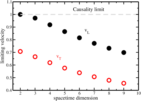
Generalizing Eq. (49) to arbitrary spacetime dimension gives

$$v_{L}^{\rm max}=\lim_{k\rightarrow\infty}\frac{d\omega}{dk}=\sqrt{c_{s}^{2}+\frac{2(D-2)}{(D-1)}\frac{\eta}{\tau_{\pi}(\epsilon+p)}+\frac{\zeta}{\tau_{\Pi}(\epsilon+p)}}\,.$$ (96)

For conformal theories, $\zeta=0$ and $c_{s}^{2}=\frac{1}{D-1}$, and using the values (95), one finds that that $v_{L}^{\rm max}$ is decreasing monotonously with $D>2$ from its maximum at $D=2$, where $v_{L}^{\rm max}$ would reach unity. The values for $v_{L}^{\rm max}$ and $v_{T}^{\rm max}$ (Eqns. (96,38), respectively) for spacetime dimensions $D<10$ are shown in Figure 1).

For $D=4$, corresponding to strongly coupled ${\cal N}=4$ SYM, also the corrections at finite (but large) coupling strength $\lambda$ to the transport coefficients have been calculated Buchel:2008sh ; Buchel:2008bz ; Buchel:2008kd ,

$$\frac{\eta}{s}=\frac{1}{4\pi}\left(1+\frac{120}{8}\zeta(3)\lambda^{-3/2}+\ldots\right),\quad\tau_{\pi}T=\frac{2-\ln 2}{2\pi}+\frac{375}{32\pi}\zeta(3)\lambda^{-3/2}+\ldots,$$

$$\kappa=\frac{\eta}{\pi T}\left(1-\frac{145}{8}\zeta(3)\lambda^{-3/2}+\ldots\right),\quad\lambda_{1}=\frac{\eta}{2\pi T}\left(1+\frac{215}{8}\zeta(3)\lambda^{-3/2}+\ldots\right)\,,$$ (97)

which lead to $v_{L}^{\rm max}\simeq 0.92-0.9796\lambda^{-3/2}$.

IV.4 Hydrodynamics of weakly coupled systems and discussion

Weakly coupled theories in general have a well defined quasiparticle structure and hence it is expected that the hydrodynamic properties of these theories are captured by kinetic theory. In particular, it is known that kinetic theory correctly reproduces the results from finite temperature quantum field theories, in the hard-thermal-loop (resummed one-loop) approximation Blaizot:2001nr . As a consequence, one would expect that the dynamics of weakly coupled quantum field theories in the hydrodynamic limit are well captured by the Müller-Israel-Stewart theory derived via kinetic theory in section III. Comparing Eq. (91) to Eq. (79) — and recalling the approximation used to derive (79) — one finds

$$\tau_{\pi}=\frac{6}{T}\frac{\eta}{s},\quad\lambda_{1}=\eta\tau_{\pi}+T^{2}{\cal O}(1),\quad\lambda_{2}=-2\eta\tau_{\pi},\quad\lambda_{3}=0,\quad\kappa=0\,,$$ (98)

where ${\cal O}(1)$ reflects the unknown contribution to $\lambda_{1}$ from the collision term and $\kappa=0$ stems from rederiving Eq. (79) in curved space Baier:2007ix . First order transport coefficients have been calculated in the weak-coupling limit for high temperature gauge theories Arnold:2003zc , in particular ${\cal N}=4$ SYM Huot:2006ys

$$\frac{\eta}{s}=\frac{6.174}{\lambda^{2}\ln{\left(2.36\lambda^{-1/2}\right)}}\,.$$ (99)

More recently, all second-order transport coefficients were evaluated consistently in QCD and scalar field theories at weak coupling York:2008rr ; Romatschke:2009ng ,

$$\tau_{\pi}=\frac{5.0\ldots 5.9}{T}\frac{\eta}{s},\quad\lambda_{1}=\frac{4.1\ldots 5.2}{T}\frac{\eta^{2}}{s},\quad\lambda_{2}=-2\eta\tau_{\pi},\quad\lambda_{3}=0,\quad\kappa=\frac{5\ s}{8\pi^{2}T}\,,$$ (100)

where the range of values indicate the dependence on the coupling constant $g$ (see Ref. York:2008rr for details). Note that the results from Eq. (79) agree reasonably well with the full calculation Eq. (100). In particular, the value of the relaxation time $\tau_{\pi}$ is such that the limiting velocity $v_{L}^{\rm max}$ is smaller than for strongly coupled systems.

Comparing the results (100) to those obtained for strongly coupled theories (95), one finds that $\lambda_{3}$ always vanishes. This could indicate that there is an additional, unidentified symmetry in conformal hydrodynamics that forces this coefficient to be zero. Moreover, a direct calculation shows that the value of $\kappa$ is beyond the accuracy of kinetic theory York:2008rr ; Moore ; Romatschke:2009ng . This indicates that the kinetic theory result is not general enough to capture the dynamics of conformal fluids in the hydrodynamic limit for arbitrary coupling, at least when spacetime is curved (since $\kappa$ couples only to the Riemann and Ricci tensor, it does not contribute to Eq. (23) when spacetime is flat; however, $\kappa$ does enter in correlators for the energy-momentum tensor in flat space Baier:2007ix ). A possible reason for this could be the fact that kinetic theory itself is only a gradient expansion to first order of the underlying quantum field theory Blaizot:2001nr , thereby possibly missing second-order contributions.

Furthermore, one finds that $\lambda_{1,2}$ have the same sign for both kinetic theory and the strongly coupled systems studied, which could indicate that the sign of these coefficients does not depend on the coupling. Finally, the fact that $v_{L}^{\rm max}$ never exceeds unity for infinitely strongly coupled theories, for theories at large (but finite) coupling, and at weak coupling, suggests, but does not prove, that causality in a second-order conformal hydrodynamics description is obeyed. At this time, there is only a proof for theories that have dual description in terms of Gauss-Bonnet gravity, where it has been shown that causality in second order hydrodynamics follows from the causality of the field theory itself Buchel:2009tt . As a consequence, one may hope that the system of equations (23),(91) constitutes a valid starting point to attempt a description of real (but nearly conformal) laboratory fluids at relativistic speeds. This application of the viscous hydrodynamic theory to high energy nuclear physics will be discussed in section V.

IV.5 Non-conformal hydrodynamics

Since most quantum field theories that successfully describe nature are not conformal theories, one may ask how deviations from conformality change the hydrodynamic equations. In particular, one may ask how important non-conformal terms not included in Eq. (91) are once conformal symmetry is slightly violated. To this end, consider the specific example of a SU(N) gauge theory at high temperature which has a trace anomaly Braun:2003rp ,

$$T^{\mu}_{\mu}=g_{\mu\nu}T^{\mu\nu}=\langle\frac{\beta(g_{\rm YM})}{2g_{\rm YM}}g^{\mu\alpha}g^{\nu\beta}F^{a}_{\mu\nu}F^{a}_{\alpha\beta}\rangle_{T}+W[g_{\mu\nu}]\,,\quad F^{a}_{\mu\nu}=\partial_{\mu}A_{\nu}^{a}-\partial_{\nu}A_{\mu}^{a}-g_{\rm YM}\,f_{abc}A^{b}_{\mu}A^{c}_{\nu}\,,$$ (101)

where $f_{abc}$ are the SU(N) structure constants, $A_{\mu}^{a}$ are the gauge fields and $\langle\rangle_{T}$ denotes the thermal quantum field theory average. Similar to section IV.2, the Weyl anomaly $W[g_{\mu\nu}]$ is not important for what follows and will be ignored. The change of the gauge theory coupling $g_{\rm YM}$ when changing the renormalization scale $\Lambda$ is given by the beta-function,

$$\Lambda\frac{\partial g_{\rm YM}}{\partial\Lambda}=\beta(g_{\rm YM})\,$$ (102)

which for weakly coupled SU(N) gauge theories is given by Gross:1973id

$$\beta(g_{\rm YM})=-\frac{11\,N}{3}\frac{g_{\rm YM}^{3}}{16\pi^{2}}+{\cal O}(g_{\rm YM}^{5})\,.$$ (103)

In fact, Eq. (101) can be derived from the gauge theory action when performing a Weyl transformation (84) of the partition function and noting that the renormalization scale changes according to $\Lambda\rightarrow e^{w(x)}\Lambda$,

$$\frac{\delta\ln Z}{\delta g_{\mu\nu}}\propto\sqrt{-g}T^{\mu\nu}\,,$$ (104)

where $g$ is the determinant of the metric $g_{\mu\nu}$ (not to be confused with $g_{\rm YM}$). Taking another functional derivative of the trace anomaly Baier:2007ix leads to

$$\frac{\delta}{\delta g_{\alpha\beta}(y)}\left(\sqrt{-g}g_{\mu\nu}(x)T^{\mu\nu}\right) = \sqrt{-g}T^{\alpha\beta}\delta(x-y)+g_{\mu\nu}(x)\frac{\delta}{\delta g_{\alpha\beta}(y)}\left(\sqrt{-g}T^{\mu\nu}\right)$$ (105)

$$= \sqrt{-g}T^{\alpha\beta}\delta(x-y)+g_{\mu\nu}(x)\frac{\delta}{\delta g_{\mu\nu}(y)}\left(\sqrt{-g}T^{\alpha\beta}\right)$$

$$= \sqrt{-g}\left(3T^{\alpha\beta}\delta(x-y)+g_{\mu\nu}\frac{\delta T^{\alpha\beta}(x)}{\delta g^{\mu\nu}(y)}\right)\,,$$

where the symmetry of the second derivative of the partition function with respect to the metric (cf. Eq. (104)) was used. On the other hand, using Eq.(101) one finds

$$\frac{\delta}{\delta g_{\alpha\beta}(y)}\left(\sqrt{-g}g_{\mu\nu}(x)T^{\mu\nu}\right) = \sqrt{-g}\langle\frac{\beta(g_{\rm YM})}{g_{\rm YM}}\left(\frac{g^{\alpha\beta}}{4}F^{\mu\nu}_{a}F_{\mu\nu}^{a}-F_{a}^{\alpha\lambda}F^{\beta}_{\ \lambda,a}\right)\rangle_{T}\delta(x-y)+{\cal O}(g_{\rm YM}^{6})\,,$$ (106)

$$= {\cal O}(g_{\rm YM}^{2})\,,$$

so that for Weyl transformations (84) this implies

$$-2g_{\mu\nu}\frac{\delta T^{\alpha\beta}(x)}{\delta g^{\mu\nu}(y)}=\frac{\delta T^{\alpha\beta}}{\delta w(y)}=6T^{\alpha\beta}\delta(x-y)+{\cal O}(g_{\rm YM}^{2})\,,\quad T^{\alpha}_{\alpha}=\epsilon-3p={\cal O}(g_{\rm YM}^{2})\,.$$ (107)

Note that an exact calculation gives $T^{\alpha}_{\alpha}={\cal O}(g_{\rm YM}^{4})$ for weakly coupled SU(N) gauge theories Moore:2008ws . Recalling that all terms in Eq. (91) transform as $\delta T^{\alpha\beta}/\delta w(y)\rightarrow 6T^{\alpha\beta}\delta(x-y)$, it becomes clear that terms not included in Eq. (91) must be ${\cal O}(g_{\rm YM}^{2})$, or in other words are small in the weak-coupling limit where SU(N) gauge theory is almost conformal. For instance, when neglecting quark masses, bulk viscosity in QCD turns out to be smaller than shear viscosity by a factor of $g_{\rm YM}^{8}$ Arnold:2006fz .

For weakly coupled systems, the form of the non-conformal hydrodynamic equations has been investigated in Betz:2008me from kinetic theory, but the second-order transport coefficients are not known to date.

For strongly coupled systems, Ref. Kanitscheider:2009as offers a beautiful example of non-conformal theories obtained by dimensional reduction of conformal theories. Starting with a conformal theory in $2\sigma>D$, and reducing to $D$ spacetime dimensions, gives an explicit realization of a relativistic hydrodynamic theory where the conformal invariance is (strongly) broken. In particular, for this theory the bulk viscosity coefficient $\zeta$ is related to shear shear viscosity as

$$\frac{\zeta}{s}=2\frac{\eta}{s}\left(\frac{1}{D-1}-c_{s}^{2}\right),$$ (108)

and the speed of sound depends on the dimension of the original theory, $c_{s}=\sqrt{\frac{1}{2\sigma-1}}$. The relaxation time in the bulk sector $\tau_{\Pi}$ equals that for the shear sector,

$$\tau_{\Pi}=\tau_{\pi},$$ (109)

so that one obtains for the limiting velocity Eq. (96)

$$v_{L}^{\rm max}=\sqrt{c_{s}^{2}\left(1-\frac{2\eta}{\tau_{\pi}(\epsilon+p)}\right)+\frac{2\eta}{\tau_{\pi}(\epsilon+p)}}\,.$$ (110)

Using the results found in section IV.3, $\frac{2\eta}{\tau_{\pi}(\epsilon+p)}$ is maximal in the limit of $D\rightarrow 2$, where $\frac{2\eta}{\tau_{\pi}(\epsilon+p)}\rightarrow 1$. In this limit, $v_{L}^{\rm max}\rightarrow 1$, regardless of the value of $c_{s}^{2}$. For $D>2$, $\frac{2\eta}{\tau_{\pi}(\epsilon+p)}<1$ and hence $v_{L}^{\rm max}$ is maximal for the largest possible value of $c_{s}^{2}$, which is $c_{s}^{2}=\frac{1}{D-1}$. As a consequence, one finds that for this class of strongly coupled theories where conformal symmetry is broken ($\zeta>0$) the limiting velocity — despite the appearance of Eq. (96) — is actually smaller than for a conformal theory in the same number of spacetime dimensions, and in particular always smaller than the speed of light. Again, while this does not proof that causality is always obeyed in second-order hydrodynamics, it adds to the list of known theories where “by coincidence” this turns out to be the case.

See Ref. Romatschke:2009kr for a complete classification of all second-order structures in the energy-momentum tensor for non-conformal fluids.

V Applying hydrodynamics to high energy nuclear collisions

V.1 Heavy-Ion Collision Primer

Figure 2: Left: Particle density (number of particles per unit rapidity, normalized by system size) as a function of collision energy (figure from Ref. Back:2004je ). Right: The energy density of QCD, calculated using lattice gauge theory, shows a strong rise close to the QCD deconfinement temperature (figure from Cheng:2007jq ).

Relativistic collisions of heavy ions (nuclei with an atomic weight heavier than carbon) offer one of the few possibilities to study nuclear matter under extreme conditions in a laboratory. The defining parameters for heavy-ion collisions are the center-of-mass collision energy per nucleon pair $\sqrt{s}$ and the geometry of the colliding nuclei (gold nuclei are typically larger than copper, and uranium nuclei are not spherically symmetric). The collisions are said to be relativistic once the center-of-mass energy is larger than the rest mass of the nuclei, or equivalently if $\sqrt{s}/2$ is larger than the nucleon mass. For the Lorentz $\gamma$ factor of the collision, this implies

$$\gamma=\frac{m\gamma c^{2}}{mc^{2}}=\frac{E^{\rm total}}{m}\simeq\frac{\sqrt{s}}{2{\rm GeV}}\,,$$ (111)

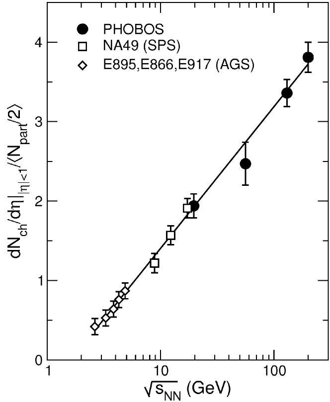
so typically $\gamma>1$. Experiments at Brookhaven National Laboratory (AGS, RHIC) and CERN (SPS) have provided a wealth of data for Au+Au collisions (AGS, RHIC) and Pb+Pb collisions (SPS) ranging in energy from $\sqrt{s}\sim 2.5-4.3$ GeV at the AGS over $\sqrt{s}\sim 8-17.3$ GeV at the SPS to $\sqrt{s}\sim 130-200$ GeV at RHIC. It was found that the number density of particles produced in these collisions increases substantially for larger $\sqrt{s}$, indicating a similar rise in the energy density Back:2004je , that may allow the study of nuclear matter above the deconfinement transition (see Figure 2).

For Au+Au collisions at RHIC, the highest energy heavy-ion collisions achieved so far, two beams of gold nuclei were accelerated in opposite directions in the RHIC ring and brought to collide once they reached their design energies. For an energy of $\sqrt{s}=200$ GeV, Eq. (111) indicates that before the collision the individual gold nuclei are highly Lorentz-contracted in the laboratory frame. Thus, rather than picturing the collisions of two spheres, one can should think of two “pancake”-like objects approaching and ultimately colliding with each other. As a consequence, the duration of the collision itself (which is on the order of the nuclear radius divided by the Lorentz gamma factor) is much shorter than the nuclear radius divided by the speed of light. Therefore, early after the collision the evolution in the directions transverse to the initial beam direction (the “transverse plane”) can be assumed to be static, and the dynamics is dominated by the longitudinal expansion of the system.

Figure 3: Schematic view of a relativistic heavy-ion collision. See text for details.

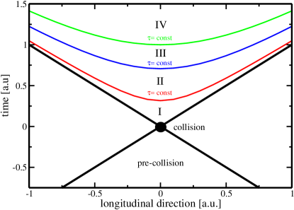
Being interested in the bulk dynamics of the matter created in a relativistic heavy-ion collision, one can divide the evolution into four stages in proper time $\tau=\sqrt{t^{2}-z^{2}}$, shown schematically in figure 3. Stage I immediately following the collision is the pre-equilibrium stage characterized by strong gradients and possibly strong gauge fields Iancu:2003xm , where a hydrodynamic description is not applicable. The duration of this stage is unknown since the process of equilibration in QCD at realistic values of the coupling is not understood, but it is generally assumed to last about $1$ fm/c. Stage II is the near-equilibrium regime characterized by small gradients where hydrodynamics should be applicable if the local temperature is well above the deconfinement transition. This stage lasts about $5-10$ fm/c, until the system becomes too dilute for equilibrium to be maintained and enters stage III, the hadron gas regime. The hadron gas is characterized by a comparatively large viscosity coefficient Prakash:1993bt , making it ill suited to be described by hydrodynamics, but well approximated by kinetic theory Bass:2000ib . This stage ends when the hadron scattering cross sections become too low and particles stop interacting. In stage IV, hadrons then fly on straight lines (free streaming) until they reach the detector.

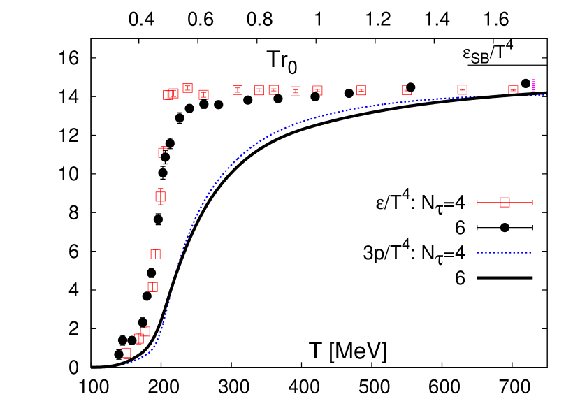
Assuming the system created by a relativistic collision of two heavy ions becomes nearly equilibrated at some instant $\tau=\tau_{0}$ in proper time, the subsequent bulk dynamics in stage II should be governed by the hydrodynamic equations (23),(91), amended by relevant non-conformal terms. To simplify the discussion, in the following these non-conformal terms will be neglected, and thus strictly speaking I will not be dealing with real heavy-ion collisions but QCD matter in the conformal approximation. However, since the conformal anomaly Eq. (107) is small except for a region close to the QCD phase transition Boyd:1996bx , there is some hope that this approximation does capture most of the important dynamics of real heavy-ion collisions.

To describe the fluid dynamics stage following a heavy-ion collision, one needs to specify the value of the hydrodynamic degrees of freedom $\epsilon,p,u^{\mu},\pi^{\mu\nu}$ at $\tau=\tau_{0}$, the equation of state $p=p(\epsilon)$, the transport coefficients $\eta,\tau_{\pi},\lambda_{1,2,3}$ governing the evolution (91) as well as a decoupling procedure to the hadron gas stage at the end of the hydrodynamic evolution. None of these are known from first principles, so one typically has to resort to models which will be described in the following sections.

V.2 Bjorken flow

The physics of relativistic heavy-ion collisions has been strongly influenced by Bjorken’s notion of “boost-invariance” Bjorken:1982qr , or the statement that at a (longitudinal) distance $z$ away from the point of (and time $t$ after) the collision, the matter should be moving with a velocity $v^{z}=z/t$. Neglecting transverse dynamics ($v^{x}=v^{y}=0$) and introducing Milne coordinates proper time $\tau=\sqrt{t^{2}-z^{2}}$ and spacetime rapidity $\xi={\rm arctanh}(z/t)$, boost-invariance for hydrodynamics simply translates into

$$u^{z}=\frac{z}{\tau}\,,\quad u^{\xi}=-u^{t}\frac{\sinh{\xi}}{\tau}+u^{z}\frac{\cosh{\xi}}{\tau}=0$$ (112)

and as a consequence $\epsilon,p,u^{\mu},\pi^{\mu\nu}$ are all independent of $\xi$, and therefore unchanged when performing a Lorentz-boost.

Even though in this highly simplified model the hydrodynamic degrees of freedom now only depend on proper time $\tau$, the system dynamics is not entirely trivial. The reason for this is that in Milne coordinates, the metric is given by $g_{\mu\nu}={\rm diag}(1,-1,-1,-\tau^{2})$ and hence is no longer coordinate-invariant. Indeed, one finds that the Christoffel symbols (IV.2) are non-zero,

$$\Gamma^{\xi}_{\xi\tau}=\frac{1}{\tau}\,,\qquad\Gamma^{\tau}_{\xi\xi}=\tau$$ (113)

so as a consequence the covariant fluid gradients are non-vanishing

$$\nabla_{\mu}u^{\mu}=\partial_{\mu}u^{\mu}+\Gamma^{\mu}_{\mu\nu}u^{\nu}=\Gamma^{\xi}_{\xi\tau}u^{\tau}=\frac{1}{\tau}\neq 0\,,$$ (114)

even though the fluid velocities are constant $u^{\mu}=(1,\vec{0})$ ! In essence, the Milne coordinate system describes a space-time that is expanding one-dimensionally, so that a system at rest within these coordinates “feels” gradients from the “stretching” of spacetime, akin to the effect of Hubble expansion in cosmology. Unlike in cosmology, however, the spacetime described by Milne coordinate is flat, as can be verified by showing that the Ricci scalar $R=0$. This is important, since one does not want to describe heavy-ion collisions in curved spacetime, but rather use the Milne coordinates as a convenient way to implement the rapid longitudinal expansion following heavy-ion collisions. Indeed, the covariant fluid gradient in Milne coordinates is precisely the same as the one from Bjorken’s boost-invariance hypothesis,

$$\nabla_{\mu}u^{\mu}=\frac{1}{\tau}=\partial_{t}\frac{t}{\tau}+\partial_{z}\frac{z}{\tau}.$$ (115)

This longitudinal flow (or “Bjorken flow”), together with the assumption $u^{x}=u^{y}=0$, can be seen as a toy model for the hydrodynamic stage following the collision of two infinitely large, homogeneous nuclei. The initial conditions for hydrodynamics at $\tau=\tau_{0}$ are then completely specified by two numbers: the initial energy density $\epsilon(\tau_{0})$ and one component of the viscous stress tensor, e.g. $\pi^{\xi}_{\xi}(\tau_{0})$ (the other components of $\pi^{\mu}_{\mu}$ are completely determined by symmetries as well as $u_{\mu}\pi^{\mu\nu}=\pi^{\mu}_{\mu}=0$). For example, in ideal hydrodynamics one finds (cf. Eq. (23))

$$D\epsilon+(\epsilon+p)\nabla_{\mu}u^{\mu}=\partial_{\tau}\epsilon+\frac{\epsilon+p}{\tau}=0\,$$ (116)

for the evolution of the energy density (the evolution equations for $Du^{\alpha}$ are trivially satisfied). For an equation of state with a constant speed of sound $c_{s}$ this can be solved analytically to give

$$\epsilon(\tau)=\epsilon(\tau_{0})\left(\frac{\tau_{0}}{\tau}\right)^{1+c_{s}^{2}}.$$ (117)

Therefore, the energy density is decreasing from its starting value because of the longitudinal system expansion, with an exponent that depends on the value of the speed of sound. For an ideal gas of relativistic particles $c_{s}^{2}=1/3$, giving rise to the behavior $\epsilon\propto\tau^{-4/3}$ that is sometimes used in heavy-ion phenomenology.

Figure 4: Rapidity dependence of produced particles (pions), for different collision energies (figure from Ref. Back:2004je ). Even at highest energies, a plateau at $Y=0$ (boost-invariance) does not seem to emerge.

Viscous corrections to Eq. (117) have been calculated in first order viscous hydrodynamics Danielewicz:1984ww ; Kouno:1989ps (the acausality problem discussed in section II.2 does not appear for Bjorken flow due to the trivial fluid velocities), as well as second order viscous hydrodynamics Muronga:2001zk ; Baier:2006um ; Luzum:2008cw , where the equations become

$$\partial_{\tau}\epsilon = -\frac{\epsilon+p}{\tau}+\frac{\pi^{\xi}_{\xi}}{\tau}$$

$$\partial_{\tau}\pi^{\xi}_{\xi} = -\frac{\pi^{\xi}_{\xi}}{\tau_{\pi}}+\frac{4\eta}{3\tau_{\pi}\tau}-\frac{4}{3\tau}\pi^{\xi}_{\xi}-\frac{\lambda_{1}}{2\tau_{\pi}\eta^{2}}\left(\pi^{\xi}_{\xi}\right)^{2}.$$ (118)

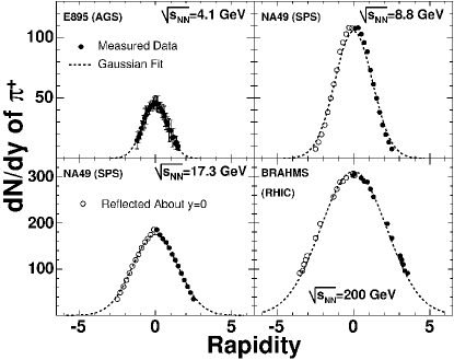
Moreover, higher order corrections are accessible for known supergravity duals to gauge theories Heller:2008mb ; Kinoshita:2008dq . Due to its simplicity, one can expect that Bjorken flow will continue to be used as a toy model of a heavy-ion collisions also in the future, and indeed also I will assume rapidity-independence for the remainder of the discussion on the hydrodynamic descriptions for simplification. However, it is imperative to recall that experimental data by no means supports Bjorken’s hypothesis of rapidity independence, as is shown in Fig. 4. Rather, the data suggests that the rapidity shape of produced particles is approximately Gaussian, independent of the collision energy. This clearly limits the applicability of the boost-invariance assumption to the central rapidity region (close to the peak of the Gaussian in Fig. 4).

V.3 Initial conditions for a hydrodynamic description of heavy-ion collisions

While pure Bjorken flow assumes matter to be homogeneous and static in the transverse (${\bf x_{\perp}}=(x,y)$) directions, a more realistic model of a heavy-ion collision will have to include the dynamics in the transverse plane. This means one has to specify the initial values for the hydrodynamic degrees of freedom as a function of ${\bf x_{\perp}}$. While it is customarily assumed that the fluid velocities initially vanish, $u^{x}(\tau_{0},{\bf x_{\perp}})=u^{y}(\tau_{0},{\bf x_{\perp}})=0$, there are two main models for the initial energy density profile $\epsilon(\tau_{0},{\bf x_{\perp}})$: the Glauber and Color-Glass-Condensate (CGC) model, respectively.

The main building block for both models is the charge density of nuclei which can be parameterized by the Woods-Saxon potential,

$$\rho_{A}(\vec{x})=\frac{\rho_{0}}{1+\exp[(|{\vec{x}}|-R_{0})/a_{0}]},$$ (119)

where $R_{0},a_{0}$ are the nuclear radius and skin thickness parameter, which for a gold nucleus take values of $R_{0}\sim 6.4$ fm and $a_{0}\sim 0.54$ fm. $\rho_{0}$ is an overall constant that is determined by requiring $\int d^{3}x\rho_{A}({\vec{x}})=A$, where $A$ is the atomic weight of the nucleus ($A\sim 197$ for gold). In a relativistic nuclear collision, the nuclei appear highly Lorentz contracted in the laboratory frame, so it is useful to define the “thickness function”

$$T_{A}({\bf x_{\perp}})=\int_{-\infty}^{\infty}dz\rho_{A}({\vec{x}}),$$ (120)

which corresponds to “squeezing” the nucleus charge density into a thin sheet.

Figure 5: Left: Number of participants $N_{\rm part}$ in the Glauber model as a function of impact parameter $b$. Right: Spatial eccentricity and area of the overlap region for the Glauber and CGC model, as a function of $N_{\rm part}$.

In its simplest version, the Glauber model for the initial energy density profile following the collision of two nuclei at an energy $\sqrt{s}$ with impact parameter $b$ is then given by

$$\epsilon({\bf x_{\perp}},b)={\rm const}\times T_{A}(x+\frac{b}{2},y)\times T_{A}(x-\frac{b}{2},y)\times\sigma_{NN}(\sqrt{s})\,,$$ (121)

where $\sigma_{NN}(\sqrt{s})$ is the nucleon-nucleon cross section and the constant is freely adjustable (see Kolb:2001qz for more complicated versions of the Glauber model). Eq. (121) has the geometric interpretation that the energy deposited at position ${\bf x_{\perp}}$ is proportional to the number of binary collisions, given by the number of charges at ${\bf x_{\perp}}$ in one nucleus times the number of charges at this position in the other nucleus, times the probability that these charges hit each other at energy $\sqrt{s}$. Another concept often used in heavy-ion collision literature is the number of participants $N_{\rm part}(b)=\int d^{2}x_{\perp}n_{\rm Part}({\bf x_{\perp}},b)$, where

$$n_{\rm Part}({\bf x_{\perp}},b) = n_{\rm Part}^{A}({\bf x_{\perp}},b)+n_{\rm Part}^{A}({\bf x_{\perp}},-b)\,$$

$$n_{\rm Part}^{A}({\bf x_{\perp}},b) = T_{A}\left(x+\frac{b}{2},y\right)\left[1-\left(1-\frac{\sigma_{NN}T_{A}\left(x-\frac{b}{2},y\right)}{A}\right)^{A}\right]\,.$$ (122)

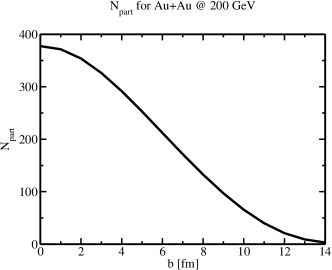
Experiments are able to determine the number of participants, but cannot access the impact parameter of a heavy-ion collision directly, so the Glauber model $N_{\rm part}$ rather than $b$ is customarily used to characterize the centrality of a collision (see Figure 5).

Figure 6: Schematic view of a heavy-ion collision at impact parameter $b$ in the transverse plane (Figure from Heinz:2009xj ).

The CGC model is based on the fact that a nucleus consists of quarks and gluons which will interact according to the laws of QCD. Accordingly, one expects corrections to the geometric Glauber model due to the non-linear nature of the QCD interactions. Heuristically, one can understand this as follows Kharzeev:2000ph : At relativistic energies, the nucleus in the laboratory frame is contracted into a sheet, so all the discussion focuses on the dynamics in the transverse plane. There, the area $\pi r_{gl}^{2}$ of a gluon is related to its momentum $Q$ via the uncertainty principle, $|r_{gl}|\times|Q|\sim\hbar=1$, and the cross-section of gluon-gluon scattering in QCD is therefore

$$\sigma\sim\alpha_{s}(Q^{2})\pi r_{gl}^{2}\sim\alpha_{s}(Q^{2})\frac{\pi}{Q^{2}}\,,$$ (123)

where $\alpha_{s}$ is the strong coupling constant. The total number of gluons can be taken to be roughly proportional to the number of partons in a nucleus, and hence also to its atomic weight $A$. Therefore, the density of gluons in the transverse plane is approximately $A/(\pi R_{0}^{2})$, where $R_{0}$ is again the nuclear radius. Gluons will start to interact with each other if the scattering probability becomes of order unity,

$$1\sim\frac{A}{\pi R_{0}^{2}}\sigma=\alpha_{s}(Q^{2})\frac{A}{R_{0}^{2}Q^{2}}\,.$$ (124)

Therefore, one finds that there is a typical momentum scale $Q_{s}^{2}=\alpha_{s}\frac{A}{R_{0}^{2}}$ which separates perturbative phenomena ($Q^{2}\gg Q_{s}^{2}$) from non-perturbative physics at $Q^{2}\ll Q_{s}^{2}$ (sometimes referred to as “saturation”). The Color-Glass-Condensate was invented McLerran:1993ni ; McLerran:1993ka to include the saturation physics at low momenta $Q^{2}$ in high energy nuclear collisions. Due to the high occupation number at low momenta, this physics turns out to be well approximated by classical chromodynamics. Despite encouraging progress Lappi:2006xc , the problem of calculating the energy density distribution in the transverse plane at $\tau=\tau_{0}$ using the Color-Glass-Condensate has not been solved, the main obstacle being the presence of non-abelian plasma instabilities Romatschke:2005pm ; Fukushima:2006ax . As a consequence, there only exist phenomenological models for the transverse energy distribution in the CGC (which are quite successful in describing experimental data, cf. Kharzeev:2002ei ), in particular the model by Ref. Dumitru:2007qr , which will be referred to as CGC model in the following.

In the CGC model, the transverse energy profile at $\tau=\tau_{0}$ is given by

$$\epsilon({\bf x_{\perp}},b)={\rm const}\times\left[\frac{dN_{g}}{d^{2}{\bf x}_{T}dY}({\bf x}_{T},b)\right]^{4/3}\,$$ (125)

where $N_{g}$ is the number of gluons produced in the collision,

$$\frac{dN_{g}}{d^{2}{\bf x}_{T}dY} \sim \int\frac{d^{2}{\bf p}_{T}}{p^{2}_{T}}\int^{p_{T}}d^{2}{\bf k}_{T}\;\alpha_{s}(k_{T})\;\phi_{+}\left(\frac{({\bf p}_{T}+{\bf k}_{T})^{2}}{4};{\bf x}_{T}\right)\;\phi_{-}\left(\frac{({\bf p}_{T}-{\bf k}_{T})^{2}}{4};{\bf x}_{T}\right)$$

$$\phi_{\pm}(k^{2}_{T};{\bf x}_{T}) = \frac{1}{\alpha_{s}(Q^{2}_{s})}\frac{Q^{2}_{s}}{\textrm{max}(Q^{2}_{s},k^{2}_{T})}\,\left(\frac{n_{\rm part}^{A}({\bf x_{\perp}},\pm b)}{T_{A}(x\pm b/2,y)}\right)(1-x)^{4}\,$$

$$Q_{s}^{2}(x,{\bf x_{\perp}}) = \frac{2\,T_{A}^{2}(x\pm b/2,y)\,{\rm GeV}^{2}}{n_{\rm part}^{A}({\bf x_{\perp}},\pm b)}\left(\frac{{\rm fm}^{2}}{1.53}\right)\left(\frac{0.01}{x}\right)^{0.288}\,,\qquad x=\frac{p_{T}}{\sqrt{s}}.$$ (126)

In order to see the difference between the Glauber and CGC model, one defines the spatial eccentricity

$$e_{x}(b)=\frac{\langle y^{2}-x^{2}\rangle_{\epsilon}}{\langle y^{2}+x^{2}\rangle_{\epsilon}},$$ (127)

and overlap area

$$S_{\rm overlap}(b)=\pi\sqrt{\langle x^{2}\rangle_{\epsilon}\langle y^{2}\rangle_{\epsilon}}\,$$ (128)

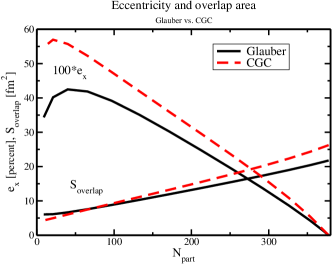
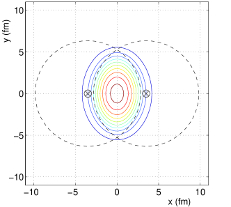
where $\langle\rangle_{\epsilon}$ denote integration over the transverse plane with weight $\epsilon({\bf x_{\perp}},b)$. These quantities characterize the shape of the energy density profile in the transverse plane (cf. Fig. 6) and are shown in Fig. 5. One finds that the CGC model typically has a larger eccentricity than the Glauber model, which will turn out to have consequences for the subsequent hydrodynamic evolution. To see this, note that if $e_{x}>0$, the energy density drops more quickly in the x-direction than in the y-direction because the overlap region is shaped elliptically. Using an equation of state $p=p(\epsilon)$ this implies that the mean pressure gradients are unequal, $\partial_{x}p>\partial_{y}p$, and according to the hydrodynamic equations (23) one expects a larger fluid velocity to build up in the x-direction than in the y-direction. Since the CGC model has a larger $e_{x}$ than the Glauber model, this anisotropy in the fluid velocities should be larger for the CGC model, as will be verified below.

V.4 Numerical solution of hydrodynamic equations

The hydrodynamic equations are a set of coupled partial differential equations with known initial conditions. Typically, it is not known how to find analytic solutions to these set of equations, so it is necessary to come up with numerical algorithms capable of solving the hydrodynamic equations. As a toy problem, it is useful to study cases where the equations simplify, e.g. the assumption of Bjorken flow discussed in section V.2 where the hydrodynamic equations become a set of ordinary differential equations (118). A standard algorithm to solve Eqns. (118) numerically is to discretize time, $\tau=\tau_{0}+n\times\Delta\tau$, where $\tau_{0}$ is the starting value, $n$ is an integer, and $\Delta\tau$ is the step-size that has to be chosen small enough for the algorithm to be accurate, but large enough for the overall computing time to be reasonable. With this discretization, derivatives become finite differences, e.g.

$$\partial_{\tau}\epsilon(\tau)=\frac{\epsilon_{n+1}-\epsilon_{n}}{\Delta\tau}\,,$$ (129)

and (118) becomes

$$\epsilon_{n+1} = \epsilon_{n}+\Delta\tau\left(-\frac{\epsilon_{n}+p_{n}}{\tau_{0}+n\Delta\tau}+\frac{\pi^{\xi}_{\xi,n}}{\tau_{0}+n\Delta\tau}\right)\,,$$ (130)

$$\pi^{\xi}_{\xi,n+1} = \pi^{\xi}_{\xi,n}+\Delta\tau\left(-\frac{\pi^{\xi}_{\xi,n}}{\tau_{\pi}}+\frac{4\eta}{3\tau_{\pi}(\tau_{0}+n\Delta\tau)}-\frac{4}{3(\tau_{0}+n\Delta\tau)}\pi^{\xi}_{\xi,n}-\frac{\lambda_{1}}{2\tau_{\pi}\eta^{2}}\left(\pi^{\xi}_{\xi,n}\right)^{2}\right)\,,$$

where for simplicity $\eta,\tau_{\pi},\lambda_{1}$ were assumed to be independent of time. Knowing $\epsilon,p,\pi^{\xi}_{\xi}$ at step $n$, the r.h.s. of the above equations are explicitly known (the reason for this was the choice of “forward-differencing” (129)) and hence one can calculate $\epsilon,p,\pi^{\xi}_{\xi}$ at step $(n+1)$. Repetition of this process gives a numerical solution for given stepsize $\Delta\tau$. Since the physical solution should be independent from the step size, it is highly recommended to create several numerical solutions for different $\Delta\tau$ and observe their convergence to a “continuum solution” for $\Delta\tau\rightarrow 0$.

Unfortunately, the above strategy of simple discretization does not always lead to a well-behaved continuum solution. To see this, consider as another toy problem the numerical solution $f(t,x)$ to the partial differential equation

$$\partial_{t}f(t,x)=-a_{0}\partial_{x}f(t,x),$$ (131)

where $a_{0}$ is assumed to be constant. Again discretizing time and space as $t=t_{0}+n\Delta t,x=m\Delta x$, the derivatives can be approximated by the finite differences

$$\partial_{t}f(t,x)=\frac{f_{n+1,m}-f_{n,m}}{\Delta t}\,,\qquad\partial_{x}f(t,x)=\frac{f_{n,m+1}-f_{n,m-1}}{2\Delta x}\,,$$ (132)

which gives rise to the “forward-time, centered-space” or “FTCS” algorithm NR §19. This algorithm is simple, allows explicit integration of the differential equations as in Eq. (V.4), and usually does not work because it is numerically unstable. The instability can be easily identified by making a Fourier-mode ansatz for $f(t,x)=e^{i\omega n\Delta t-ikm\Delta x}$ and calculating the dispersion relation $\omega=\omega(k)$ from the FTCS-discretized Eq. (131)

$$\frac{f_{n+1,m}-f_{n,m}}{\Delta t}=f_{n,m}\frac{e^{i\omega\Delta t}-1}{\Delta t}=-a_{0}\frac{f_{n,m+1}-f_{n,m-1}}{2\Delta x}=f_{n,m}\frac{ia_{0}}{\Delta x}\sin k\Delta x\,.$$ (133)

One finds

$${\rm Im}\ \omega(k)=-\frac{1}{2\Delta t}\ln\left[1+\left(a_{0}\frac{\Delta t}{\Delta x}\right)^{2}\sin^{2}k\Delta x\right]<0\,$$ (134)

which signals exponential growth in $f(t,x)$ for all modes $k$. As a consequence, any numerical solution to Eq. (131) using the FTCS algorithm will become unstable after a finite simulation time set by the inverse of Eq. (134).

However, this instability can be cured by choosing a slightly different way of calculating the time derivative, namely replacing $f_{n,m}$ in Eq. (132) by its space average $\frac{1}{2}(f_{n,m+1}+f_{n,m-1})$,

$$\partial_{t}f(t,x)=\frac{f_{n+1,m}-f_{n,m}}{\Delta t}-\frac{f_{n,m+1}-2f_{n,m}+f_{n,m-1}}{2\Delta t}\,.$$ (135)

This algorithm, known as the “LAX” scheme NR §19, has a dispersion relation with

$${\rm Im}\ \omega(k)=-\frac{1}{2\Delta t}\ln\left[\cos^{2}k\Delta x+\left(a_{0}\frac{\Delta t}{\Delta x}\right)^{2}\sin^{2}k\Delta x\right]\,$$ (136)

and hence is numerically stable for $a_{0}\frac{\Delta t}{\Delta x}<1$, e.g. for sufficiently small time steps $\Delta t$. The stability of the LAX scheme comes from the presence of the last term in Eq. (135), which in “continuum-form” is a second derivative that leads to

$$\partial_{t}f(t,x)=-a_{0}\partial_{x}f(t,x)+\frac{(\Delta x)^{2}}{2\Delta t}\partial_{x}^{2}f(t,x)$$ (137)

instead of Eq. (131). For sufficiently small $\Delta x$, this equation reduces to the original equation, so the LAX algorithm indeed converges to the physically interesting solution. But the presence of this extra term, which is crucial for the numerical stability, also has a physical interpretation: comparing Eq. (137) to the diffusion equation (33) one is led to interpret the coefficient $\frac{(\Delta x)^{2}}{2\Delta t}$ as “numerical viscosity”. The LAX scheme works where the FTCS scheme fails because the viscous term dampens the instabilities, in much the same way that the turbulent instability in fluids is damped by the viscous terms LL §26. Indeed, for ideal fluid dynamics numerical viscosity is essential for stabilizing the numerical algorithms. On the other hand, viscous fluid dynamics comes with real viscosity inbuilt, so it is tempting to conjecture that as long as $\eta$ or $\zeta$ are finite and $\Delta t$ is sufficiently small, numerical viscosity is not needed to stabilize the numerical algorithm for solving the hydrodynamic equations, and the simple FTCS scheme can be used. Indeed, at least for the problem of heavy-ion collision, this strategy leads to a stable algorithm Baier:2006gy ; Romatschke:2007jx ; Romatschke:2007mq ; codedown .

Figure 7: Left to right: snapshots at $\tau=1,3$ and $7$ fm/c of the temperature profile $T(x,y)$ for a hydrodynamic simulation of a $\sqrt{s}=200$ GeV Au+Au collision at $b=10$ fm. The initial spatial eccentricity is gradually converted into momentum eccentricity and almost disappears at late times.

Aiming to solve the hydrodynamic equations in the transverse plane (assuming boost-invariance in the longitudinal direction), one first has to choose a set of independent hydrodynamic degrees of freedom, e.g., $\epsilon,u^{x},u^{y},\pi^{xx},\pi^{xy},\pi^{yy}$ for which initial conditions are provided along the lines of section V.3. Only time derivatives to first order of these six quantities enter the coupled partial differential equations (23),(91), so that formally one can write the hydrodynamic equations in matrix form

$${\bf A}\cdot\left(\begin{array}[]{c}\partial_{\tau}\epsilon\\ \partial_{\tau}u^{x}\\ \ldots\\ \partial_{\tau}\Pi^{yy}\end{array}\right)={\bf b}\,,$$ (138)

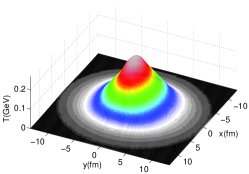
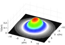
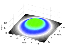
where ${\bf A},{\bf b}$ are a matrix and vector with coefficients that do not involve time derivatives. Using the FTCS scheme to discretize derivatives, and matrix inversion to solve (138), the value of the independent hydrodynamic degrees of freedom at the next time step are explicitly given in terms of known quantities (once the equation of state and hydrodynamic transport coefficients are specified). Reconstructing all hydrodynamic fields from the independent components and repetition of the above procedure then leads to a numerical solution for the hydrodynamic evolution of a heavy-ion collision for given $\Delta\tau,\Delta x$ as long as $\eta>0$ (in practice, values as low as $\eta/s\sim 10^{-4}$ are stable with reasonable $\Delta\tau$). The convergence of these numerical solutions to the continuum limit is explicitly observed when choosing a series of sufficiently small step sizes $\Delta\tau,\Delta x$. Snapshots of the temperature profile in a typical simulation are shown in Fig. 7.

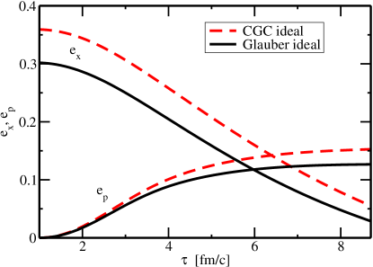
Fig. 7 also displays the gradual reduction of the eccentricity (the shape of the temperature profile in the transverse plane becomes more and more circular as time progresses). The eccentricity corresponds to a spatial anisotropy in the pressure gradients which is converted by hydrodynamics into a momentum anisotropy (fluid velocities $u^{x}\neq u^{y}$). In analogy to the definition of the spatial eccentricity (127), it is therefore useful to introduce the concept of momentum anisotropy

$$e_{p}(b)=\frac{\int d^{2}{\bf x_{\perp}}T^{xx}-T^{yy}}{\int d^{2}{\bf x_{\perp}}T^{xx}+T^{yy}}\,.$$ (139)

The time evolution of the eccentricity and momentum anisotropy in the Glauber and CGC model are shown in Fig. 8. As discussed in section V.3, the higher initial eccentricity in the CGC model gets converted in a larger momentum anisotropy.

Figure 8: Time evolution of the spatial and momentum anisotropies, Eq. (127) and Eq. (139), respectively, in the Glauber and CGC model for a $\sqrt{s}=200$ GeV Au+Au collision at $b=7$ fm (Figure from Luzum:2008cw ).

V.5 Freeze-out

Experiments in relativistic nuclear collisions measure momentum distributions of particles (pions, kaons, protons, etc.), whereas hydrodynamics deals with energy density, pressure and fluid velocities. Clearly, in order to make contact with experiment, the hydrodynamic degrees of freedom need to be converted into measurable quantities, which is often called the “freeze-out”. The connection between hydrodynamics and particle degrees of freedom is provided by kinetic theory, which was discussed in section III. In particular, one requires the hydrodynamic and kinetic theory energy momentum tensor at freeze-out to be the same,

$$T^{\mu\nu}_{\rm kinetic\ theory}=\int d\chi p^{\mu}p^{\nu}f(\vec{p},t,\vec{x})=T^{\mu\nu}_{\rm hydro}\,,$$ (140)

where for small departures from equilibrium the explicit form of $f$ in terms of hydrodynamic degrees of freedom is provided by Eq. (59). Once $f(\vec{p},t,\vec{x})$ is known, one can construct the particle current from kinetic theory

$$n^{\mu}=\int d\chi p^{\mu}f(\vec{p},t,\vec{x})\,,$$ (141)

which will be used to construct particle spectra that can be compared to experimental measurements.

Freeze-out from hydrodynamic to particle degrees of freedom is expected to occur when the interactions are no longer strong enough to keep the system close to thermal equilibrium. Below the QCD phase transition, this happens, e.g., when the system cools and viscosity increases Prakash:1993bt until the viscous corrections in (59) become too large and a fluid dynamic description is no longer valid. In practice, this is hard to implement, so simplified approaches such as isochronous and isothermal freeze-out are often used (see, however, Hung:1997du; Dusling:2007gi ). All of these have in common that they define a three dimensional hypersurface $\Sigma$ with a normal vector $d\Sigma^{\mu}$ such that the total number of particles after freeze-out is given by the particle current (141) leaving the hypersurface $\Sigma^{\mu}$,

$$N=\int n^{\mu}d\Sigma_{\mu}=\int d\chi f(\vec{p},t,\vec{x})p^{\mu}d\Sigma_{\mu}\,.$$ (142)

For energy densities sufficiently below the QCD phase transition, the energy momentum tensor is well approximated by a non-interacting hadron resonance gas Karsch:2003vd . This translates to

$$d\chi=\sum_{i}(2s_{i}+1)(2g_{i}+1)\frac{d^{4}p}{(2\pi)^{3}}\delta(p^{\mu}p_{\mu}-m_{i}^{2})2\theta(p^{0}),$$ (143)

where the sum is over all known hadron resonances Amsler:2008zzb and $s_{i},g_{i}$ are the spin and isospin of a resonance with mass $m_{i}$. As a consequence,

$$N=\sum_{i}\int d^{3}p\frac{1}{\sqrt{m_{i}^{2}+\vec{p}^{\,2}}}\left(p^{0}\frac{dN}{d^{3}p}\right)_{i}\,,$$ (144)

where

$$\left(p^{0}\frac{dN}{d^{3}p}\right)_{i}=\frac{d_{i}}{(2\pi)^{3}}\int d\Sigma_{\mu}p^{\mu}f(\vec{p},t,\vec{x})\,,\quad d_{i}=(2s_{i}+1)(2g_{i}+1)\,,$$ (145)

is the single-particle spectrum for the resonance $i$. Eq. (145) is the generalization of the “Cooper-Frye freeze-out prescription” CooperFrye to viscous fluids with $f$ given by Eq. (65).

Arguably the simplest model is isochronous freeze-out, where the system is assumed to convert to particles at a given constant time (or proper time). While fairly unrealistic, it allows a rather intuitive introduction of the general freeze-out formalism: constant time defines $\Sigma^{\mu}(t,x,y,z)$ in the hydrodynamic evolution which is parametrized by $t={\rm const}$. The normal vector $d\Sigma^{\mu}$ on this hypersurface is given by Ruuskanen:1986py ; Rischke:1996em

$$d\Sigma_{\mu}=\epsilon_{\mu\alpha\beta\gamma}\frac{\partial\Sigma^{\alpha}}{\partial x}\frac{\partial\Sigma^{\beta}}{\partial y}\frac{\partial\Sigma^{\gamma}}{\partial z}dxdydz\,,$$ (146)

where $\epsilon_{\mu\alpha\beta\gamma}$ is the totally antisymmetric tensor in four dimensions with $\epsilon_{0123}=+1$. A simple calculation gives $d\Sigma^{\mu}=(1,\vec{0})d^{3}x$ and therefore the momentum particle spectra are easily obtained by integration of the distribution function,

$$p^{\mu}d\Sigma^{\mu}=p^{0}d^{3}x\,,\qquad\left(\frac{dN}{d^{3}p}\right)_{i}=\frac{d_{i}}{(2\pi)^{3}}\int d^{3}xf(\vec{p},t={\rm const},\vec{x})\,.$$ (147)

Slightly more realistic is isochronous freeze-out in proper time, $\tau={\rm const}$, where the freeze-out surface $\Sigma^{\mu}=(\tau\cosh{\xi},x,y,\tau\sinh{\xi})$ is parametrized by $x,y,\xi$, because this incorporates Bjorken flow. Introducing rapidity $Y={\rm arctanh}{(p^{z}/p^{0})}$ and $m_{\perp}=\sqrt{m^{2}+p_{\perp}^{2}}$ for convenience, a short calculation for the normal vector $d\Sigma^{\mu}$ gives Luzum:2008cw

$$d\Sigma_{\mu}p^{\mu}=\tau m_{\perp}\cosh{(Y-\xi)}dxdyd\xi\,.$$ (148)

Considering for illustration a Boltzmann gas in equilibrium with $f_{\rm eq}=\exp{[-p^{\mu}u_{\mu}/T]}$, for vanishing spatial fluid velocities one has

$$p^{0}\left(\frac{dN}{d^{3}p}\right)_{i} = \frac{d_{i}}{(2\pi)^{3}}\tau m_{\perp}\int dxdyd\xi\cosh{(Y-\xi)}\exp{[-m_{\perp}\cosh{(Y-\xi)}/T]}$$ (149)

$$= \frac{2d_{i}}{(2\pi)^{2}}\tau m_{\perp}\int drrK_{1}\left(\frac{m_{\perp}}{T}\right)\,,$$

while for non-vanishing fluid velocities with azimuthal symmetry ($u^{x}(r)=u^{y}(r)=u^{r}(r)/\sqrt{2}$) a short calculation gives Baier:2006gy

$$p^{0}\left(\frac{dN}{d^{3}p}\right)_{i}=\frac{2d_{i}}{(2\pi)^{2}}\tau m_{\perp}\int drrK_{1}\left(\frac{m_{\perp}u^{\tau}}{T}\right)I_{0}\left(\frac{|{\bf p_{\perp}}|u^{r}}{T}\right)\,,$$ (150)

where $K(z),I(z)$ are modified Bessel functions and the transverse radius $r=\sqrt{x^{2}+y^{2}}$ has been introduced for convenience. Comparing the integrands in Eq. (149),(150) when transverse momenta $p_{\perp}=|{\bf p_{\perp}}|$ are much larger than the temperature $T$ or mass $m$, one finds

$$\frac{K_{1}(m_{\perp}/T)}{K_{1}(m_{\perp}u^{\tau}/T)I_{0}(p_{\perp}u^{r}/T)}\sim\frac{\exp{[(m_{\perp}(1-u^{\tau})+p_{\perp}u^{r})/T]}}{u^{\tau}u^{r}p_{\perp}/T}\gg 1$$ (151)

if $u^{r}\sim{\cal O}(1)$. This means that the presence of $u^{r}>0$, or “radial flow”, leads to particle spectra which are “flatter” at large $p_{T}$. This is confirmed by numerical simulations Huovinen:2006jp .

For a Boltzmann gas out of equilibrium and Bjorken flow only ($u^{\tau}=1,u^{i}=0$) the viscous correction to the distribution function (65) is

$$\frac{\pi^{\mu\nu}p_{\mu}p_{\nu}}{2(\epsilon+p)T^{2}}=\frac{(\pi^{xx}+\pi^{yy})p_{\perp}^{2}+2\pi^{\xi\xi}m_{\perp}^{2}/\tau^{2}\sinh^{2}{(Y-\xi)}}{4(\epsilon+p)T^{2}}=\frac{\pi^{\xi}_{\xi}\left(p_{\perp}^{2}-2m_{\perp}^{2}\sinh^{2}{(Y-\xi)}\right)}{4(\epsilon+p)T^{2}}\,,$$ (152)

so that the single particle spectrum becomes Baier:2006um

$$p^{0}\left(\frac{dN}{d^{3}p}\right)_{i}=\frac{2d_{i}}{(2\pi)^{2}}\tau m_{\perp}\int drr\left[K_{1}\left(\frac{m_{\perp}}{T}\right)+\pi^{\xi}_{\xi}\,\frac{p_{\perp}^{2}K_{1}\left(\frac{m_{\perp}}{T}\right)-2m_{\perp}TK_{2}\left(\frac{m_{\perp}}{T}\right)}{4(\epsilon+p)T^{2}}\right]\,.$$ (153)

Since for Bjorken flow typically $\pi^{\xi}_{\xi}>0$, this implies that viscous corrections tend to have the same effect of making particle spectra flatter at large $p_{T}$, which hints at the difficulty of extracting viscosity and radial flow from experimental data Romatschke:2007jx . More information is needed to disentangle these effects, so one decomposes the particle spectra into a Fourier series with respect to the azimuthal angle in momentum $\phi_{p}=\arctan\left(p^{y}/p^{x}\right)$ Kolb:2003zi ,

$$\left(p^{0}\frac{dN}{d^{3}p}\right)_{i}=v_{0}(|{\bf p_{\perp}}|,b)\left[1+2v_{2}(|{\bf p_{\perp}}|,b)\cos{2\phi_{p}}+2v_{4}(|{\bf p_{\perp}}|,b)\cos{4\phi_{p}}+\ldots\right]\,,$$ (154)

where the coefficients $v_{2},v_{4}$ are referred to as “elliptic” and “hexadecupole” flow Ollitrault:1992bk , respectively. $v_{2},v_{4}$ and even higher harmonics were measured experimentally for $\sqrt{s}=200$ GeV Au+Au collisions Adams:2003zg and may be useful to distinguish between flow and viscous effects.

Figure 9: Entropy per particle as a function of temperature for a gas of a realistic set of massive resonances with Bose-Einstein/Fermi-Dirac statistics (dotted line). Also shown are results when approximating by Boltzmann statistics (dashed line) and total initial entropy over final multiplicity from a numerical hydrodynamics simulation with isothermal freeze-out using Boltzmann statistics Luzum:2008cw (squares). The numerical results prior to the decay of unstable resonances is in fair agreement with the analytic prediction. The decay of unstable resonances produces additional particles, leading to a smaller ratio of initial entropy to final multiplicity (circles).

A more realistic criterion than isochronous freeze-out is to assume decoupling at a predefined temperature (isothermal freeze-out). In this case the hypersurface $\Sigma$ can be parametrized by $\xi$, $\phi={\rm arctan}{\frac{y}{x}}$ and a time-like coordinate $0\leq c\leq 1$ with $c=0$ corresponding to the center $x=y=0$ of the transverse plane. Assuming boost-invariance in the longitudinal direction, this leads to $\Sigma^{\mu}=\Sigma^{\mu}(\tau(c)\cosh\xi,x(c,\phi),y(c,\phi),\tau(c)\sinh\xi)$, and the normal vector is evaluated analogous to Eq. (146) (cf.Luzum:2008cw ). The resulting single particle spectra are then given by Eq. (145), where it may be convenient to change variables $c=\frac{\tau_{fo}-\tau}{\tau_{fo}-\tau_{0}}$ in the integral

$$\int_{0}^{1}dc=-\int_{\tau_{0}}^{\tau_{fo}}\frac{d\tau}{\tau_{fo}-\tau_{0}}\,,$$ (155)

where $\tau_{0},\tau_{fo}$ correspond to the start and end of the hydrodynamic evolution. For isothermal freeze-out at a temperature $T_{fo}$, kinetic theory specifies the entropy density $s=\frac{\epsilon+p}{T_{\rm fo}}$ and the number density $n=n^{\mu}u_{\mu}$ of particles. In particular, for a massive Boltzmann gas in equilibrium Eq. (57),(141) lead to

$$s=\sum_{i}\frac{(2s_{i}+1)(2g_{i}+1)}{2\pi^{2}}m_{i}^{3}K_{3}\left(\frac{m_{i}}{T_{\rm fo}}\right),\quad n=\sum_{i}\frac{(2s_{i}+1)(2g_{i}+1)}{2\pi^{2}}m_{i}^{2}T_{\rm fo}K_{2}\left(\frac{m_{i}}{T_{\rm fo}}\right)\,$$ (156)

which can be used to quantify $s/n$, the amount of entropy each resonance degree of freedom is carrying. For extremely high temperatures $s/n\rightarrow 4$, which is the known limit for a gas of massless relativistic particles Gyulassy:1983ub , but for temperatures below the QCD phase transition and a realistic set of hadron resonances Amsler:2008zzb , $s/n$ depends on $T_{\rm fo}$ (see Fig. 9). For ideal hydrodynamics the total entropy $S$ in the fluid is conserved (27), and hence the total number of particles $N$ created by an isothermal freeze-out should be given by $N=\frac{n}{s}S$, which provides a non-trivial check on numerical codes.

After freeze-out, the hadron gas dynamics may be described by a hadron cascade code such as Bass:2000ib . A more simplistic approach is to assume that particles stop interacting after freeze-out, but unstable particles are allowed to decay, which changes the spectra of stable particles Sollfrank:1990qz ; Sollfrank:1991xm . The decay of unstable resonances can be simulated using public codes such as OSCAR and leads to particle production, as can be seen in Fig. 9.

V.6 Viscous effects and open problems

Ideal hydrodynamic simulations have been used quite successfully in the past to describe the properties of the particle spectra produced in relativistic heavy-ion collisions Back:2004je ; Adcox:2004mh ; Arsene:2004fa ; Adams:2005dq (for reviews, see e.g. Huovinen:2006jp ; Kolb:2003dz ). Viscous effects have only been studied more recently: the presence of viscosity leads to viscous entropy production given by Eq. (27), which increases the total multiplicity for fixed initial entropy. The amount of viscous entropy production depends on the hydrodynamic initialization time $\tau_{0}$ Dumitru:2007qr , and for $\tau_{0}\sim 1$ fm/c is on the order of $10$ percent for $\eta/s=0.08$ Romatschke:2007jx ; Song:2008si .

Figure 10: Reduction of elliptic flow coefficient due to shear viscosity: different groups agree that at $p_{\perp}=1.5$ GeV, there is a $\sim 20$ percent reduction of $v_{2}$ for $\eta/s=0.08$ (Figures from Romatschke:2007mq ; Dusling:2007gi ; Molnar:2008xj ; Song:2008si , clockwise from upper left.)

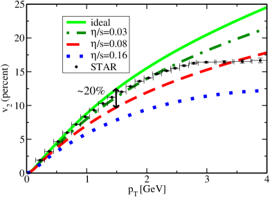
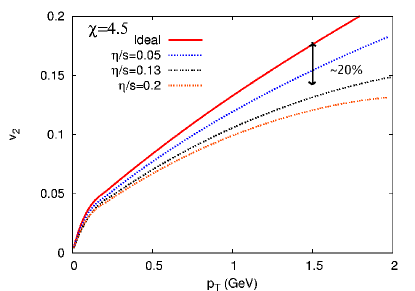
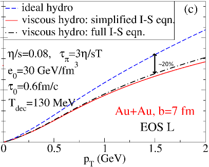
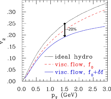
Viscosity also leads to stronger radial flow, which increases the mean transverse momentum of particles Teaney:2003kp ; Baier:2006gy ; Romatschke:2007jx . Maybe more importantly, the presence of shear viscosity strongly decreases the elliptic flow coefficient $v_{2}$. After some initial disagreement, several different groups now agree on the quantitative suppression of elliptic flow by shear viscosity, as is demonstrated in Fig. 10. Unfortunately, this does not directly constrain the $\eta/s$ of hot QCD matter because the overall size of elliptic flow (which is proportional to the final momentum anisotropy $e_{p}$) is dictated by the initial spatial eccentricity, which is unknown (cf. Fig. 8, see also Ref. Luzum:2008cw ).

Figure 11: Centrality dependence of particle spectra (multiplicity, mean momentum and elliptic flow) as well as momentum dependence of charge hadron elliptic flow, for a viscous hydrodynamic simulation of a $\sqrt{s}=200$ GeV Au+Au collision using the CGC model compared to experimental data Adler:2003cb ; Alver:2007qw ; Abelev:2008ed (Figures from Luzum:2008cw ).

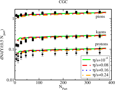
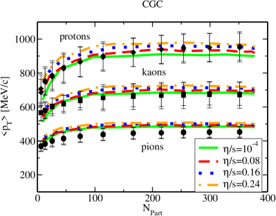
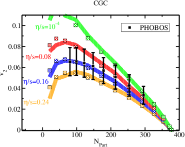
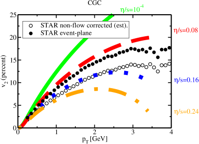
Many open problems remain, such as

• Exploring the effects of bulk viscosity. One study Karsch:2007jc suggests that bulk viscosity may become large close to the QCD phase transition (however, see Moore:2008ws ; Romatschke:2009ng ; CaronHuot:2009ns ), which would have important consequences for the hydrodynamic evolution. First phenomenological steps in this direction have been taken in Song:2008hj , but it would be worthwile to have a classification of all the non-conformal terms (including an estimate of their importance/size) in the hydrodynamic equations.

• Implementing finite baryon chemical potential in the viscous hydrodynamic simulations. On the one hand needed to describe the asymmetry in the baryon/anti-baryon multiplicities, the viscous hydrodynamic evolution in the vicinity of a possible QCD critical point could on the other hand help to guide experimental searches for this critical point (cf.Asakawa:2008ti ).

• Combining viscous hydrodynamics with a hadron cascade code to more realistically describe the freeze-out process. Ideally such a hybrid code would make the choice of a freeze-out temperature superfluous, eliminating one model parameter (cf.Teaney:2000cw ; Hirano:2005xf ; Petersen:2008dd ).

These (and other) problems are straightforward to solve in the sense that they do not require fundamentally new ideas, but “only” hard work. However, there are also at least two problems outside the framework of hydrodynamics, which would have to be solved in order to claim a complete understanding of high energy nuclear collisions:

• What is the value of the initial spatial eccentricity $e_{x}$ in high energy nuclear collision? Can it be calculated or measured without having to rely on models (Glauber/CGC)? Since the spatial eccentricity controls the amount of elliptic flow generated in a relativistic nuclear collision, knowing $e_{x}$ seems necessary to quantify the viscosity of hot nuclear matter.

• How and when does the system equilibrate? An answer to this question would give a well defined value to the hydrodynamic starting time $\tau_{0}$ as well as the eccentricity at this time. Currently both $\tau_{0}$ and $e_{x}(\tau_{0})$ are “guessed”, with no solid arguments for any particular value.

Nevertheless, the striking ability of viscous hydrodynamics to describe the momentum spectra of the majority of particles, including the elliptic flow coefficient, in the highest energy Au+Au collisions at RHIC (see Fig. 11) make relativistic nuclear collisions an ideal application for the old, new, and future developments in hydrodynamic theory.

VI Conclusions

Relativistic viscous hydrodynamics is an effective theory for the long-wavelength behavior of matter. The relativistic Navier-Stokes equation would do justice to this long-wavelength behavior, but does not lend itself easily to direct numerical simulations because of its ultraviolet behavior. Generalizations of the Navier-Stokes equation including second-order gradients have been proposed to cure this difficulty, and indeed provide a phenomenological regularization of the Navier-Stokes equation that can be simulated numerically unless the regularization parameter is too small.

Interestingly, performing a complete gradient expansion to second order reproduces this attractive feature of regularizing the Navier-Stokes equation, besides having the benefit of constituting an improved approximation of the underlying quantum field theory. For all theories where the regularization parameter obtained from this gradient expansion is known, its value is such that the ultraviolet behavior of the second-order hydrodynamic equations is benign. It is not known whether this is a coincidence.

The second order hydrodynamic equations have been applied to the problem of high energy nuclear collisions, offering a good description of the experimentally measured particle spectra at low momenta. Further work is needed to extract material parameters of hot nuclear matter, such as the shear viscosity coefficient, from experimental data.

Many other applications of second order hydrodynamics are possible, e.g. in astrophysics (viscous damping of neutron star r-modes Lindblom:2001hd ) or cosmology (effects of bulk viscosity Zimdahl:1996ka ).

Whether in the formulation I have described in these pages, or not, one thing is certain: relativistic viscous hydrodynamics is here to stay.

Appendix A Proof of Causality of Maxwell-Cattaneo type equations

Let us first establish that the diffusion-type equation

$$\partial_{t}\delta u^{y}-\frac{\eta_{0}}{\epsilon_{0}+p_{0}}\partial_{x}^{2}\delta u^{y}=f(t,x)\,,$$ (157)

which was discussed in section II.2 for the homogeneous case $f(t,x)=0$, violates causality. To this end, let us calculate the retarded Green’s function $G({\bf x},{\bf x^{\prime}})$, ${\bf x}=(t,x)$, of the differential operator (157),

$$\left[\partial_{t}-\nu\partial_{x}^{2}\right]G({\bf x},{\bf x^{\prime}})=\delta^{2}({\bf x}-{\bf x^{\prime}}),\quad\nu=\frac{\eta_{0}}{\epsilon_{0}+p_{0}}$$ (158)

Doing a Fourier-transform of $G$ one finds

$$G({\bf x},{\bf x^{\prime}})=\int\frac{d^{2}{\bf k}}{(2\pi)^{2}}\frac{e^{-i\omega(t-t^{\prime})+ik(x-x^{\prime})}}{-i\omega+\nu k^{2}}$$ (159)

which can be solved by the usual contour integration methods and Gaussian integration,

$$G({\bf x},{\bf x^{\prime}})=\frac{\theta(t-t^{\prime})}{\sqrt{4\pi\nu(t-t^{\prime})}}\exp{\left[-\frac{(x-x^{\prime})^{2}}{4\nu(t-t^{\prime})}\right]}\ .$$

The solution to Eq. (157) is then

$$\delta u^{y}(t,x)=\int d^{2}{\bf x^{\prime}}G({\bf x},{\bf x^{\prime}})f({\bf x^{\prime}})=\frac{\theta(t)}{\sqrt{4\pi\nu t}}\exp{\left[-\frac{x^{2}}{4\nu t}\right]}\,,$$ (160)

where the system was started with an initial “kick”, $f(t,x)=\delta(t)\delta(x)$. One can see that for any finite time $t>0$, the perturbation is non-vanishing for all values of $x$, not only for those $x<t$. This obviously violates causality.

Considering instead of the diffusion-type equation (157) the Maxwell-Cattaneo law

$$\partial_{t}\delta u^{y}+\frac{1}{\epsilon_{0}+p_{0}}\partial_{x}\pi^{xy}=0,\quad\tau_{\pi}\partial_{t}\pi^{xy}+\pi^{xy}=-\eta_{0}\partial_{x}\delta u^{y}\,,$$ (161)

the Green’s function has to fulfill

$$\left[\partial_{t}^{2}+\frac{\partial_{t}}{\tau_{\pi}}-\frac{\nu}{\tau_{\pi}}\partial_{x}^{2}\right]G({\bf x},{\bf x^{\prime}})=\frac{1}{\tau_{\pi}}\delta^{2}({\bf x}-{\bf x^{\prime}})$$ (162)

and hence is given by

$$G({\bf x},{\bf x^{\prime}})=\int\frac{d^{2}{\bf k}}{(2\pi)^{2}}\frac{e^{-i\omega(t-t^{\prime})+ik(x-x^{\prime})}}{-\omega^{2}\tau_{\pi}-i\omega+\nu k^{2}}\,.$$ (163)

The frequency integration proceeds as before, and one finds

$$G({\bf x},{\bf x^{\prime}})=\theta(t-t^{\prime})\int_{-\infty+i\epsilon}^{\infty+i\epsilon}\frac{dk}{2\pi}\frac{i}{\tau_{\pi}}e^{ik(x-x^{\prime})}\left[\frac{e^{-i\omega^{+}(t-t^{\prime})}-e^{-i\omega^{-}(t-t^{\prime})}}{\omega^{+}-\omega^{-}}\right]\,,$$ (164)

where $2\tau_{\pi}\omega^{\pm}=-i\pm\sqrt{4\tau_{\pi}\nu k^{2}-1}$. The integral over $k$ is chosen in the upper half-plane and the branch cut of the square-root is chosen to run from $k=-(4\tau_{\pi}\nu)^{-1/2}$ to $k=(4\tau_{\pi}\nu)^{-1/2}$ along the real axis MF1 §7.4. To evaluate the integral

$$I_{+}\equiv e^{-\frac{t-t^{\prime}}{2\tau_{\pi}}}\int_{-\infty+i\epsilon}^{\infty+i\epsilon}\frac{dk}{2\pi}\frac{i\exp{\left[ik(x-y)-i\frac{(t-t^{\prime})}{2\tau_{\pi}}\sqrt{4\tau_{\pi}\nu k^{2}-1}\right]}}{\sqrt{4\tau_{\pi}\nu k^{2}-1}}\,,$$

note that if $x>x^{\prime}+\frac{(t-t^{\prime})}{2\tau_{\pi}}\sqrt{4\tau_{\pi}\nu}$, then the contour can be closed by a semicircle in the upper half plane, giving a vanishing contribution since there are no singularities in that halfplane. For $x<x^{\prime}+\frac{(t-t^{\prime})}{2\tau_{\pi}}\sqrt{4\tau_{\pi}\nu}$ on the other hand, the contribution will not vanish. It can be calculated by using a table of Laplace transforms MF1 §7.4, MF2 §11, giving

$$I_{+}=\theta\left((t-t^{\prime})\sqrt{\frac{\nu}{\tau_{\pi}}}-(x-x^{\prime})\right)\frac{e^{-\frac{t-t^{\prime}}{2\tau_{\pi}}}}{\sqrt{4\nu\tau_{\pi}}}I_{0}\left(\sqrt{\frac{(t-t^{\prime})^{2}}{4\tau_{\pi}^{2}}-\frac{(x-x^{\prime})^{2}}{4\nu\tau_{\pi}}}\right)\,,$$ (165)

where $I_{0}(x)$ is a modified Bessel function. Similarly, one can calculate the other component of Eq. (164), so that one finds

$$G({\bf x},{\bf x^{\prime}})=\theta(t-t^{\prime})\,\theta\left(\frac{(t-t^{\prime})^{2}\nu}{\tau_{\pi}}-(x-x^{\prime})^{2}\right)\frac{e^{-\frac{t-t^{\prime}}{2\tau_{\pi}}}}{\sqrt{4\nu\tau_{\pi}}}I_{0}\left(\sqrt{\frac{(t-t^{\prime})^{2}}{4\tau_{\pi}^{2}}-\frac{(x-x^{\prime})^{2}}{4\nu\tau_{\pi}}}\right)\,.$$ (166)

Figure 12: Green’s function for the diffusion equation and Maxwell-Cattaneo law for $\tau_{\pi}=\nu$. See text for details

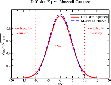
From the step-function in Eq. (166), one can easily convince oneself that the solution $\delta u^{y}(t,x)$ to Eq. (161) is confined to $|x|<t\,v_{T}^{\rm max}$, where $v_{T}^{\rm max}=\sqrt{\frac{\eta_{0}}{\tau_{\pi}(\epsilon_{0}+p_{0})}}$ coincides with the limit found in Eq. (38). The difference between the Maxwell-Cattaneo solution and the diffusion equation is highlighted in Fig. 12, where $\sqrt{4\pi\nu t}G({\bf x},{\bf 0})$ is plotted for $t=10\nu$ as a function of $x$. One can see that $G({\bf x},0)$ has non-vanishing support in the region excluded by causality for the diffusion equation, while this does not happen for the Maxwell-Cattaneo law.

Appendix B Notations and Conventions

This appendix is a collection of notations and conventions used in the main part of the article.

• The metric sign convention is $(+,-,-,-)$

• Projectors:

  $$\Delta^{\mu\nu}=g^{\mu\nu}-u^{\mu}u^{\nu}\,,\quad P^{\mu\nu}_{\alpha\beta}=\Delta^{\mu}_{\alpha}\Delta^{\nu}_{\beta}+\Delta^{\mu}_{\beta}\Delta^{\nu}_{\alpha}-\frac{2}{3}\Delta^{\mu\nu}\Delta_{\alpha\beta}\,,$$ (167)

  with properties $u_{\mu}\Delta^{\mu\nu}=u_{\mu}P^{\mu\nu}_{\alpha\beta}=0$, $g_{\mu\nu}P^{\mu\nu}_{\alpha\beta}=0$.

• Derivatives:

  $$D=u^{\mu}D_{\mu}\,,\quad\nabla_{\mu}=\Delta^{\alpha}_{\mu}D_{\mu}\,,\quad D_{\mu}=u_{\mu}D+\nabla_{\mu}\,,$$ (168)

  where $D_{\mu}$ is the geometric covariant derivative that reduces to $D_{\mu}\rightarrow\partial_{\mu}$ for flat space. In the non-relativistic, flat-space limit,

  $$D=\partial_{t}+\vec{v}\cdot\vec{\partial}+{\cal O}\left(|\vec{v}|^{2}\right)\,,\quad\vec{\nabla}=-\vec{\partial}+{\cal O}\left(|\vec{v}|\right)\,,$$ (169)

  which supports the interpretation of time-, and space-like derivatives for $D$ and $\nabla$, respectively.

• Brackets:

  $$A^{(\alpha}B^{\beta)}=\frac{1}{2}\left(A^{\alpha}B^{\beta}+A^{\beta}B^{\alpha}\right)\,,\quad A^{[\alpha}B^{\beta]}=\frac{1}{2}\left(A^{\alpha}B^{\beta}-A^{\beta}B^{\alpha}\right)\,,$$

  $$A^{<\alpha}B^{\beta>}=P^{\alpha\beta}_{\mu\nu}A^{\mu}B^{\nu}\,,$$ (170)

  which are used to define e.g. the vorticity, $\Omega_{\alpha\beta}=\nabla_{[\alpha}u_{\beta]}$. Note that the above definition of $A^{<\alpha}B^{\beta>}$ differs from others (e.g. Baier:2007ix ) by a factor of $2$.

References

- (1) L. Euler, “Principes généraux du mouvement des fluides”, Mém. Acad. Sci. Berlin 11 (1755) [printed in 1757]. Also in Opera omnia, ser. 2, 12, (1907) 54-91, E226.
- (2) L.D. Landau and E.M. Lifshitz, Course of Theoretical Physics Volume 6, “Fluid Mechanics”, Elsevier, 2nd edition (1987).
- (3) C.L.M.H. Navier, ”Mémoire sur les lois du mouvement des fluides”, Mém. Acad. Sci. Inst. France, 6, (1822), 389-440.
- (4) G.G. Stokes, “On the theories of the internal friction of fluids in motion, and of the equilibrium and motion of elastic solids”, Trans. Camb. Philos. Soc. 8:287-319 (1845).
- (5) D. T. Son and A. O. Starinets, JHEP 0603 (2006) 052 [arXiv:hep-th/0601157].
- (6) D. H. Rischke, arXiv:nucl-th/9809044.
- (7) A. Muronga, Phys. Rev. C 69 (2004) 034903 [arXiv:nucl-th/0309055].
- (8) W. A. Hiscock and L. Lindblom, Phys. Rev. D 31 (1985) 725.
- (9) P. Kostadt and M. Liu, Phys. Rev. D 62 (2000) 023003.
- (10) J.C. Maxwell, Phil. Trans. R. Soc. 157 (1867) 49.
- (11) C. Cattaneo, Atti Sem. Mat. Fis. Univ. Modena 3 (1948) 3.
- (12) D. Jou, J. Casas-Vazquez and G. Lebon, Rep. Prog. Phys. 51 (1988) 1105.
- (13) D.D. Joseph and L. Preziosi, Rev. Mod. Phys. 61 (1989) 41.
- (14) C.C. Ackerman, B. Bertman, H.A. Fairbank and R.A. Guyer, Phys. Rev. Lett. 16 (1966) 789.
- (15) I. Müller, Z. Phys. 198 (1967) 329.
- (16) W. Israel, Ann.Phys. 100 (1976) 310.
- (17) D. Jou, J. Casas-Vazquez and G. Lebon, Rep. Prog. Phys. 62 (1999) 1035.
- (18) R. Loganayagam, JHEP 0805 (2008) 087 [arXiv:0801.3701 [hep-th]].
- (19) S. Bhattacharyya et al., JHEP 0806 (2008) 055 [arXiv:0803.2526 [hep-th]].
- (20) P. Romatschke, arXiv:0906.4787 [hep-th].
- (21) L.D. Landau and E.M. Lifshitz, Course of Theoretical Physics Volume 10, “Physical Kinetics”, Pergamon Press (1981).
- (22) L. Boltzmann, Sitzb. d. Akad. d. Wiss. Wien, 66 275 (1872).
- (23) S.R. de Groot, W.A. van Leeuwen and C.G. van Weert, “Relativistic kinetic theory : principles and applications”, Elsevier North-Holland (1980).
- (24) W. Israel and J.M. Stewart, Phys. Lett. 58A (1976) 213; W. Israel and J.M. Stewart, Ann.Phys. 118, (1979) 341.
- (25) S. Chapman and T.G. Cowling, “The mathematical theory of non-uniform gases”, Cambridge University Press (1970).
- (26) H. Grad, Comm. Pure Appl. Math. 2 (1949), 331.
- (27) R. Baier, P. Romatschke and U. A. Wiedemann, Phys. Rev. C 73 (2006) 064903 [arXiv:hep-ph/0602249].
- (28) R. Baier, P. Romatschke and U. A. Wiedemann, Nucl. Phys. A 782 (2007) 313 [arXiv:nucl-th/0604006].
- (29) R. Baier, P. Romatschke, D. T. Son, A. O. Starinets and M. A. Stephanov, JHEP 0804 (2008) 100 [arXiv:0712.2451 [hep-th]].
- (30) M. J. Duff, Class. Quant. Grav. 11 (1994) 1387 [arXiv:hep-th/9308075].
- (31) O. Aharony, S. S. Gubser, J. M. Maldacena, H. Ooguri and Y. Oz, Phys. Rept. 323 (2000) 183 [arXiv:hep-th/9905111].
- (32) J. M. Maldacena, Adv. Theor. Math. Phys. 2 (1998) 231 [Int. J. Theor. Phys. 38 (1999) 1113] [arXiv:hep-th/9711200].
- (33) D. T. Son and A. O. Starinets, Ann. Rev. Nucl. Part. Sci. 57 (2007) 95 [arXiv:0704.0240 [hep-th]].
- (34) S. Bhattacharyya, V. E. Hubeny, S. Minwalla and M. Rangamani, JHEP 0802 (2008) 045 [arXiv:0712.2456 [hep-th]].
- (35) M. Natsuume and T. Okamura, Phys. Rev. D 77 (2008) 066014 [arXiv:0712.2916 [hep-th]].
- (36) M. Natsuume and T. Okamura, Prog. Theor. Phys. 120 (2008) 1217 [arXiv:0801.1797 [hep-th]].
- (37) M. Van Raamsdonk, JHEP 0805 (2008) 106 [arXiv:0802.3224 [hep-th]].
- (38) M. Haack and A. Yarom, JHEP 0810 (2008) 063 [arXiv:0806.4602 [hep-th]].
- (39) S. Bhattacharyya, R. Loganayagam, I. Mandal, S. Minwalla and A. Sharma, JHEP 0812 (2008) 116 [arXiv:0809.4272 [hep-th]].
- (40) M. Natsuume, Phys. Rev. D 78 (2008) 066010 [arXiv:0807.1392 [hep-th]].
- (41) P. Kovtun, D. T. Son and A. O. Starinets, Phys. Rev. Lett. 94 (2005) 111601 [arXiv:hep-th/0405231].
- (42) J. Erdmenger, M. Haack, M. Kaminski and A. Yarom, JHEP 0901 (2009) 055 [arXiv:0809.2488 [hep-th]].
- (43) M. Haack and A. Yarom, Nucl. Phys. B 813 (2009) 140 [arXiv:0811.1794 [hep-th]].
- (44) A. Buchel, Nucl. Phys. B 803 (2008) 166 [arXiv:0805.2683 [hep-th]].
- (45) A. Buchel and M. Paulos, Nucl. Phys. B 805 (2008) 59 [arXiv:0806.0788 [hep-th]].
- (46) A. Buchel and M. Paulos, Nucl. Phys. B 810 (2009) 40 [arXiv:0808.1601 [hep-th]].
- (47) J. P. Blaizot and E. Iancu, Phys. Rept. 359 (2002) 355 [arXiv:hep-ph/0101103].
- (48) P. Arnold, G. D. Moore and L. G. Yaffe, JHEP 0305 (2003) 051 [arXiv:hep-ph/0302165].
- (49) S. C. Huot, S. Jeon and G. D. Moore, Phys. Rev. Lett. 98 (2007) 172303 [arXiv:hep-ph/0608062].
- (50) M. A. York and G. D. Moore, arXiv:0811.0729 [hep-ph].
- (51) P. Romatschke and D. T. Son, arXiv:0903.3946 [hep-ph].
- (52) G.D. Moore, private communication.
- (53) A. Buchel and R. C. Myers, arXiv:0906.2922 [hep-th].
- (54) V. M. Braun, G. P. Korchemsky and D. Mueller, Prog. Part. Nucl. Phys. 51 (2003) 311 [arXiv:hep-ph/0306057].
- (55) D. J. Gross and F. Wilczek, Phys. Rev. Lett. 30 (1973) 1343.
- (56) G. D. Moore and O. Saremi, JHEP 0809 (2008) 015 [arXiv:0805.4201 [hep-ph]].
- (57) P. Arnold, C. Dogan and G. D. Moore, Phys. Rev. D 74 (2006) 085021 [arXiv:hep-ph/0608012].
- (58) B. Betz, D. Henkel and D. H. Rischke, arXiv:0812.1440 [nucl-th].
- (59) I. Kanitscheider and K. Skenderis, JHEP 0904 (2009) 062 [arXiv:0901.1487 [hep-th]].
- (60) B. B. Back et al., Nucl. Phys. A 757 (2005) 28 [arXiv:nucl-ex/0410022].
- (61) M. Cheng et al., Phys. Rev. D 77 (2008) 014511 [arXiv:0710.0354 [hep-lat]].
- (62) E. Iancu and R. Venugopalan, arXiv:hep-ph/0303204.
- (63) M. Prakash, M. Prakash, R. Venugopalan and G. Welke, Phys. Rept. 227 (1993) 321.
- (64) S. A. Bass and A. Dumitru, Phys. Rev. C 61 (2000) 064909 [arXiv:nucl-th/0001033].
- (65) G. Boyd, J. Engels, F. Karsch, E. Laermann, C. Legeland, M. Lutgemeier and B. Petersson, Nucl. Phys. B 469 (1996) 419 [arXiv:hep-lat/9602007].
- (66) J. D. Bjorken, Phys. Rev. D 27 (1983) 140.
- (67) P. Danielewicz and M. Gyulassy, Phys. Rev. D 31 (1985) 53.
- (68) H. Kouno, M. Maruyama, F. Takagi and K. Saito, Phys. Rev. D 41 (1990) 2903.
- (69) A. Muronga, Phys. Rev. Lett. 88 (2002) 062302 [Erratum-ibid. 89 (2002) 159901] [arXiv:nucl-th/0104064].
- (70) M. P. Heller, P. Surowka, R. Loganayagam, M. Spalinski and S. E. Vazquez, arXiv:0805.3774 [hep-th].
- (71) S. Kinoshita, S. Mukohyama, S. Nakamura and K. y. Oda, Prog. Theor. Phys. 121 (2009) 121 [arXiv:0807.3797 [hep-th]].
- (72) M. Luzum and P. Romatschke, Phys. Rev. C 78 (2008) 034915 [Erratum-ibid. C 79 (2009) 039903] [arXiv:0804.4015 [nucl-th]].
- (73) U. W. Heinz, arXiv:0901.4355 [nucl-th].
- (74) P. F. Kolb, U. W. Heinz, P. Huovinen, K. J. Eskola and K. Tuominen, Nucl. Phys. A 696 (2001) 197 [arXiv:hep-ph/0103234].
- (75) D. Kharzeev and M. Nardi, Phys. Lett. B 507 (2001) 121 [arXiv:nucl-th/0012025].
- (76) L. D. McLerran and R. Venugopalan, Phys. Rev. D 49 (1994) 2233 [arXiv:hep-ph/9309289].
- (77) L. D. McLerran and R. Venugopalan, Phys. Rev. D 49 (1994) 3352 [arXiv:hep-ph/9311205].
- (78) T. Lappi and R. Venugopalan, Phys. Rev. C 74 (2006) 054905 [arXiv:nucl-th/0609021].
- (79) P. Romatschke and R. Venugopalan, Phys. Rev. Lett. 96 (2006) 062302 [arXiv:hep-ph/0510121].
- (80) K. Fukushima, F. Gelis and L. McLerran, Nucl. Phys. A 786 (2007) 107 [arXiv:hep-ph/0610416].
- (81) D. Kharzeev, E. Levin and M. Nardi, Nucl. Phys. A 730 (2004) 448 [Erratum-ibid. A 743 (2004) 329] [arXiv:hep-ph/0212316].
- (82) A. Dumitru, E. Molnar and Y. Nara, Phys. Rev. C 76 (2007) 024910 [arXiv:0706.2203 [nucl-th]].
- (83) Numerical Recipes in C, 2nd edition, Cambridge University Press, 1992.
- (84) R. Baier and P. Romatschke, Eur. Phys. J. C 51 (2007) 677 [arXiv:nucl-th/0610108].
- (85) P. Romatschke, Eur. Phys. J. C 52 (2007) 203 [arXiv:nucl-th/0701032].
- (86) P. Romatschke and U. Romatschke, Phys. Rev. Lett. 99 (2007) 172301 [arXiv:0706.1522 [nucl-th]].
-
(87)
C++ versions of the relativistic viscous hydrodynamic
codes with and without radial symmetry may be
obtained from http://hep.itp.tuwien.ac.at/
paulrom/
%\cite{Hung:1997du}
\bibitem{Hung:1997du}
C.
M. Hung and E. V. Shuryak, Phys. Rev. C 57 (1998) 1891 [arXiv:hep-ph/9709264]. - (88) K. Dusling and D. Teaney, Phys. Rev. C 77 (2008) 034905 [arXiv:0710.5932 [nucl-th]].
- (89) P. V. Ruuskanen, Acta Phys. Polon. B 18 (1987) 551.
- (90) D. H. Rischke and M. Gyulassy, Nucl. Phys. A 608 (1996) 479 [arXiv:nucl-th/9606039].
- (91) F. Karsch, K. Redlich and A. Tawfik, Eur. Phys. J. C 29 (2003) 549 [arXiv:hep-ph/0303108].
- (92) C. Amsler et al. [Particle Data Group], Phys. Lett. B 667 (2008) 1.
- (93) F. Cooper and G. Frye, Phys. Rev. D 10 (1974) 186.
- (94) P. Huovinen and P. V. Ruuskanen, Ann. Rev. Nucl. Part. Sci. 56 (2006) 163 [arXiv:nucl-th/0605008].
- (95) P. F. Kolb, Phys. Rev. C 68 (2003) 031902 [arXiv:nucl-th/0306081].
- (96) J. Y. Ollitrault, Phys. Rev. D 46 (1992) 229.
- (97) J. Adams et al. [STAR Collaboration], Phys. Rev. Lett. 92 (2004) 062301 [arXiv:nucl-ex/0310029].
- (98) M. Gyulassy and T. Matsui, Phys. Rev. D 29 (1984) 419.
- (99) J. Sollfrank, P. Koch and U. W. Heinz, Phys. Lett. B 252 (1990) 256.
- (100) J. Sollfrank, P. Koch and U. W. Heinz, Z. Phys. C 52 (1991) 593.
- (101) AZHYDRO version 0.2, available from http://karman.physics.purdue.edu/OSCAR/
- (102) K. Adcox et al. [PHENIX Collaboration], Nucl. Phys. A 757 (2005) 184 [arXiv:nucl-ex/0410003].
- (103) I. Arsene et al. [BRAHMS Collaboration], Nucl. Phys. A 757 (2005) 1 [arXiv:nucl-ex/0410020].
- (104) J. Adams et al. [STAR Collaboration], Nucl. Phys. A 757 (2005) 102 [arXiv:nucl-ex/0501009].
- (105) P. F. Kolb and U. W. Heinz, arXiv:nucl-th/0305084.
- (106) D. Molnar and P. Huovinen, J. Phys. G 35 (2008) 104125 [arXiv:0806.1367 [nucl-th]].
- (107) H. Song and U. W. Heinz, Phys. Rev. C 78 (2008) 024902 [arXiv:0805.1756 [nucl-th]].
- (108) D. Teaney, Phys. Rev. C 68 (2003) 034913 [arXiv:nucl-th/0301099].
- (109) F. Karsch, D. Kharzeev and K. Tuchin, Phys. Lett. B 663 (2008) 217 [arXiv:0711.0914 [hep-ph]].
- (110) S. Caron-Huot, arXiv:0903.3958 [hep-ph].
- (111) H. Song and U. W. Heinz, arXiv:0812.4274 [nucl-th].
- (112) M. Asakawa, S. A. Bass, B. Muller and C. Nonaka, Phys. Rev. Lett. 101 (2008) 122302 [arXiv:0803.2449 [nucl-th]].
- (113) D. Teaney, J. Lauret and E. V. Shuryak, Phys. Rev. Lett. 86 (2001) 4783 [arXiv:nucl-th/0011058].
- (114) T. Hirano, U. W. Heinz, D. Kharzeev, R. Lacey and Y. Nara, Phys. Lett. B 636 (2006) 299 [arXiv:nucl-th/0511046].
- (115) H. Petersen, J. Steinheimer, G. Burau, M. Bleicher and H. Stocker, Phys. Rev. C 78 (2008) 044901 [arXiv:0806.1695 [nucl-th]].
- (116) L. Lindblom and B. J. Owen, Phys. Rev. D 65 (2002) 063006 [arXiv:astro-ph/0110558].
- (117) W. Zimdahl, Phys. Rev. D 53 (1996) 5483 [arXiv:astro-ph/9601189].
- (118) S. S. Adler et al. [PHENIX Collaboration], Phys. Rev. C 69 (2004) 034909 [arXiv:nucl-ex/0307022].
- (119) B. Alver et al. [PHOBOS Collaboration], Int. J. Mod. Phys. E 16 (2008) 3331 [arXiv:nucl-ex/0702036].
- (120) B.I. Abelev et al. [STAR Collaboration], arXiv:0801.3466 [nucl-ex].
- (121) P.M. Morse and H. Feshbach, “Methods of theoretical physics”, part I, McGraw-Hill (1953).
- (122) P.M. Morse and H. Feshbach, “Methods of theoretical physics”, part II, McGraw-Hill (1953).