Progress on Cosmological Magnetic Fields

Abstract

A variety of observations impose upper limits at the nano Gauss level on magnetic fields that are coherent on inter-galactic scales while blazar observations indicate a lower bound $\sim 10^{-16}$ Gauss. Such magnetic fields can play an important astrophysical role, for example at cosmic recombination and during structure formation, and also provide crucial information for particle physics in the early universe. Magnetic fields with significant energy density could have been produced at the electroweak phase transition. The evolution and survival of magnetic fields produced on sub-horizon scales in the early universe, however, depends on the magnetic helicity which is related to violation of symmetries in fundamental particle interactions. The generation of magnetic helicity requires new CP violating interactions that can be tested by accelerator experiments via decay channels of the Higgs particle.

I Introduction

Several excellent reviews on cosmological magnetic fields exist Grasso and Rubinstein (2001); Widrow (2002); Vallée (2004); Durrer and Neronov (2013); Subramanian (2016). This article is a perspective on where the subject is in 2020, on several claims and counter-claims, and on open problems of interest for the future. The focus is on physical aspects of the generation of cosmological magnetic fields, their evolution, and observation.

Let us start by discussing the generation of magnetic fields. The presence of a cosmological plasma suggests that the discussion should be based in the language of magneto-hydrodynamics (MHD), with the MHD equation (e.g. Ch. 10 in Jackson (1975)),

$$\partial_{t}{\bf B}=\nabla\times({\bf v}\times{\bf B})+\frac{1}{\sigma}\nabla^{2}{\bf B}$$ (1)

where ${\bf B}$ is the magnetic field, ${\bf v}$ the plasma velocity, and $\sigma$ the electrical conductivity of the plasma. The key point is that the plasma does not provide a source term for the magnetic field: if ${\bf B}(t=0,{\bf x})=0$ then ${\bf B}(t,{\bf x})=0$ for all times and magnetic fields cannot be generated within the MHD description.

Fortunately source terms can be present when we go beyond MHD. The charges in standard astrophysical plasmas consists of electrons and protons, which have equal and opposite electric charge but the masses are vastly different, $m_{p}\approx 2000m_{e}$. The Thomson interaction cross-sections are also vastly different: $\sigma_{e\gamma}/\sigma_{p\gamma}\approx(m_{p}/m_{e})^{2}\sim 10^{6}$. This opens up the possibility for generating electric currents when astrophysical plasmas interact with photons. For example, consider rotational flow of the cosmological medium prior to recombination. The electrons scatter more efficiently with the ambient radiation and feel a greater drag than do the protons, producing a net electric current that sources a magnetic field. Harrison Harrison (1970); Pogosian et al. (2002) has used this scheme to propose (weak) magnetic field generation if there is turbulence during cosmological recombination.

The Harrison mechanism illustrates how the violation of fundamental symmetries might play a role in the generation of magnetic fields. Crucial use is made of the violation of electric charge conjugation symmetry (C) since electrons and protons have different masses and interaction strengths with photons. The role of fundamental symmetry violations becomes even more interesting in the context of early universe cosmology and the electroweak phase transition serves as an illustration. At the electroweak epoch the cosmological medium has essentially equal numbers of particles and antiparticles and there is only very weak CP violation that distinguishes their interactions. Instead, as discussed in Sec. III, the production of magnetic fields follows from the dynamics of the Higgs field during the phase transition and it appears that the violation of fundamental symmetries is not necessary. However, there is more to the story, as the evolution and survival of cosmological magnetic fields depends critically on the helicity (circular polarization) of the magnetic field. A helical magnetic field is characterized by the quantity ${\bf B}\cdot\nabla\times{\bf B}$ and overall magnetic helicity implies that the average value of ${\bf B}\cdot\nabla\times{\bf B}$ is non-vanishing, in turn implying a violation of parity (P) and charge+parity (CP) symmetries. Therefore the present amplitude of cosmological magnetic fields that were generated at the electroweak epoch depends on the strength of P and CP symmetry violations in the fundamental interactions, just as the amount of cosmic matter-antimatter asymmetry depends on violations of these symmetries. Then the observation of cosmological magnetic fields and their helicity can inform us about fundamental symmetry violations that should also appear in accelerator experiments, thus making another important outer-space/inner-space connection.

In the cosmological context, Maxwell electrodynamics is only applicable after the electroweak phase transition (EWPT), $\sim 10^{-10}\,{\rm s}$ after the big bang. Prior to the EWPT, there were 3 SU(2) (“weak”) gauge fields and 1 U(1) (“hypercharge”) gauge field and electromagnetism was undefined. Once the electroweak $SU(2)\times U(1$) symmetry is broken, only one of the gauge fields remains massless and is what we call the electromagnetic gauge field. Although the electroweak model may be unfamiliar to non-particle physicists, since the discovery of the Higgs particle the model is about as robust as Maxwell’s electrodynamics. There are sure to be some extensions but the basic equations are firm. So predictions from the electroweak equations can be made with similar confidence as from Maxwell equations, and if the electroweak equations generate magnetic fields at the EWPT, they are as real as say the cosmic microwave background.

I will discuss the generation of magnetic fields at the EWPT in some detail in Sec. III.1. It is important to note that electromagnetism as derived from the electroweak model has magnetic sources (magnetic monopoles) and ${\rm div}({\bf B})\neq 0$ in general. Once the Higgs has acquired a non-zero vacuum expectation value (VEV) everywhere and the EWPT is complete, we recover Maxwell’s equations and MHD. During the EWPT the full electroweak dynamics needs to be taken into account. This opens up new research problems – How can one include plasma effects in the electroweak model? Is there a suitable “non-Abelian MHD” approximation applicable to the electroweak plasma? How do results depend on “unknowns” such as neutrino masses, dark matter, additional sources of CP violation?

The ultimate test of all theoretical ideas is whether they are confirmed by experiment or observations. For cosmological magnetic fields there has been a lot of progress on the observational front. Some decades ago, Faraday rotation of quasars placed the most stringent constraints on cosmological magnetic fields. Now there are additional constraints from the cosmic microwave background and from blazar gamma ray data. Importantly, blazar observations place lower bounds on magnetic fields provided our understanding of electron/positron propagation in the cosmological medium is correct. Blazar observations can in principle be used to detect magnetic helicity and the spectra of magnetic fields. This topic is discussed in Sec. II.

The presence of magnetic fields may impact our understanding of other cosmological epochs. Already there is discussion of whether magnetic fields can affect faster Hydrogen recombination and potentially resolve the tension in the low redshift Hubble constant measurements with those using the CMB Jedamzik and Pogosian (2020). The interactions of hypothesized neutrino magnetic moments with primordial magnetic fields may affect big bang nucleosynthesis Enqvist et al. (1993, 1995) and have consequences for neutrino detection experiments Baym and Peng (2021). There may be other effects waiting to be discovered – do magnetic fields affect the QCD phase transition? do they leave an imprint on the 21 cm observations? do they affect structure formation? And, very importantly, can they help explain the observed magnetic fields in galaxies and clusters of galaxies?

There already are attempts to answer a large number of these questions. As in all good science, there are claims and counter-claims, making this a fertile ground for research, innovative ideas, and further experiments and observations. The purpose of this progress report is to give a perspective on the salient results and discussions.

After setting up some basic conventions and notation in Sec. I.1, I start in Sec. II by discussing some (not all) observational efforts, focusing on blazar observations as these appear to be most promising at present. In Sec. III, I discuss the generation of magnetic fields in the early universe, focusing on the production during the EWPT. Then I come to a summary of the evolution of cosmological magnetic fields in Sec. IV. Finally, in Sec. V, I discuss a few other ideas for generating and amplifying magnetic fields. Here I also discuss the possibility that magnetic fields may indicate new fundamental interactions and that these could be tested in accelerator experiments.

We use natural units ($\hbar=1=c$) throughout, Lorentz-Heaviside conventions for electromagnetism, and a flat Friedman-Robertson-Walker cosmology. For numerical estimates, conversions between different units are neatly summarized in con .

I.1 Framework: stochastic, statistically isotropic magnetic fields

We can imagine a uniform magnetic field that pervades the universe. However, this cannot be the outcome of a local, dynamical process since locality implies that magnetic field directions in vastly separated regions are governed by independent physics. We will only consider such local processes in this report. Then we are interested in stochastic magnetic fields that on average are isotropic. The correlation function for any divergence-free stochastic vector field that is statistically isotropic can be written as Monin and Yaglom (1975),

$$\langle B_{i}({\bf x}+{\bf r})B_{j}({\bf x})\rangle=M_{N}(r)P_{ij}+M_{L}(r){\hat{r}}_{i}{\hat{r}}_{j}+\epsilon_{ijk}r_{k}M_{H}(r)$$ (2)

where $P_{ij}=\delta_{ij}-{\hat{r}}_{i}{\hat{r}}_{j}$ is the projection tensor orthogonal to ${\hat{r}}$; $M_{N}$, $M_{L}$ and $M_{H}$ are respectively the “normal”, “longitudinal” and “helical” parts of the correlation function. Since $\nabla\cdot{\bf B}=0$, we have a relation between the normal and longitudinal spectra

$$M_{N}(r)=\frac{1}{2r}\frac{d}{dr}\left(r^{2}M_{L}(r)\right)$$ (3)

With the Fourier transform conventions,

$${\bf b}({\bf k})=\int d^{3}x\,{\bf B}({\bf x})e^{+i{\bf k}\cdot{\bf x}},\ {\bf B}({\bf x})=\int\frac{d^{3}k}{(2\pi)^{3}}{\bf b}({\bf k})e^{-i{\bf k}\cdot{\bf x}}$$ (4)

the k-space correlator takes the form,

$$\langle b_{i}({\bf k})b_{j}^{*}({\bf k}^{\prime})\rangle=\left[\frac{E_{M}(k)}{4\pi k^{2}}p_{ij}+i\epsilon_{ijl}k^{l}\frac{H_{M}(k)}{8\pi k^{2}}\right]$$ (5)

$$\hskip-85.35826pt\times(2\pi)^{6}\delta^{(3)}({\bf k}-{\bf k}^{\prime})$$

where $p_{ij}=\delta_{ij}-{\hat{k}}_{i}{\hat{k}}_{j}$. $E_{M}(k)$ is called the “power spectrum” and $H_{M}(k)$ the “helicity spectrum” (or sometimes the “helicity power spectrum”). Commonly encountered spectra in the cosmology literature are the “Batchelor spectrum” with $E_{M}(k)\propto k^{4}$ and the “scale invariant” spectrum with $E_{M}(k)\propto k^{-1}$.

The correlators refer to an ensemble average over many stochastic realizations of the magnetic field. To connect theory and observations, since we only have one realization of the magnetic field in the universe, the ensemble average is to be thought of as a spatial average (the “ergodic hypothesis”),

$$\langle B_{i}({\bf x}+{\bf r})B_{j}({\bf x})\rangle\to\frac{1}{V}\int_{V}d^{3}x\,B_{i}({\bf x}+{\bf r})B_{j}({\bf x})$$ (6)

where $V$ is some large volume. This assumes that the spatial separations ($r$) of interest are smaller than the extent of the integration volume.

The $x$-space and $k$-space correlation functions can be related,

$$M_{N}(r)+\frac{1}{2}M_{L}(r)=\int_{0}^{\infty}dk\,E_{M}(k)\frac{\sin(kr)}{kr}$$ (7)

with $M_{N}$ and $M_{L}$ related as in (3), and

$$M_{H}(r)=-\frac{1}{2r}\int_{0}^{\infty}dk\,kH_{M}(k)\frac{d}{d(kr)}\left(\frac{\sin(kr)}{kr}\right)$$ (8)

A clarification regarding “magnetic helicity” is necessary. Magnetic helicity is defined as

$${\rm magnetic\ helicity}\equiv\int d^{3}x\,{\bf A}\cdot{\bf B}$$ (9)

where the integral is over all space. (In a finite volume, the expression is gauge invariant provided the magnetic field is orthogonal to the areal vector everywhere on the boundary of the volume.) Magnetic helicity has an interpretation in terms of the linking number (or writhe and twist) of magnetic flux lines Moreau (1961); Moffatt (1969); Berger and Field (1984). Magnetic helicity is a very useful quantity because it is conserved in MHD evolution of plasmas with high electrical conductivity. Even if the electrical conductivity is finite, helicity conservation is observed in numerical solutions and has been used to explain experimental results Taylor (1974). However, magnetic helicity is a non-local quantity and hence is not experimentally measurable. Instead the “physical magnetic helicity” defined as ${\bf B}\cdot\nabla\times{\bf B}$ is local and measurable. From (2) we derive,

$$\langle{\bf B}\cdot\nabla\times{\bf B}\rangle=6M_{H}(0)=\int_{0}^{\infty}dk\,k^{2}H_{M}(k)$$ (10)

where the last relation can be derived using (8).

Observations only probe an averaged value of inter-galactic magnetic fields. Since the magnetic field is a three-vector, there are several ways to define the “average magnetic field strength” Enqvist and Olesen (1993); Hindmarsh and Everett (1998). For example, the line-averaged magnetic field strength on a curve of length $L$ may be defined as,

$${\bar{B}}_{\rm line}=\frac{1}{L}\int_{0}^{L}d{\bf l}\cdot{\bf B}$$ (11)

and one may further average over a set of such curves. In the literature, one also encounters an “effective” magnetic field based on the averaged energy density,

$$B_{\rm eff}^{2}=\frac{1}{V}\int_{V}d^{3}x\,{\bf B}^{2}$$ (12)

Following Durrer and Neronov Durrer and Neronov (2013), we may also define the “magnetic field strength on scale $\lambda$”,

$$B_{\lambda}\equiv\sqrt{2kE_{M}(k)}$$ (13)

where $\lambda\equiv 2\pi/k$. In contrast, the Planck collaboration Planck Collaboration et al. (2016) defines the magnetic field strength smoothed on a scale $\lambda$ as

$${\cal B}_{\lambda}^{2}=\int_{0}^{\infty}\frac{dk\,k^{2}}{2\pi^{2}}e^{-\lambda^{2}k^{2}}P_{B}(k)$$ (14)

where, to bridge conventions,

$$P_{B}(k)=2(2\pi)^{3}\frac{E_{M}(k)}{4\pi k^{2}}.$$ (15)

Another definition advocated in Hindmarsh and Everett (1998) is the volume averaged magnetic field,

$${\bf B}_{V}=\frac{1}{V}\int_{V}d^{3}x\,{\bf B}({\bf x}).$$ (16)

If the volume is chosen to be a sphere of radius $\lambda$ we can express the root-mean-square of ${\bf B}_{V}$ in terms of $E_{M}(k)$,

$$B_{V,\lambda}^{2}=2\int dk\,E_{M}(k)W^{2}_{V}(k)$$ (17)

where

$$W_{V}(k)=\frac{3}{(k\lambda)^{3}}(\sin(k\lambda)-k\lambda\cos(k\lambda))$$ (18)

The window function $W^{2}_{V}(k)$ in (17) limits the integration to regions with $k\lesssim 1/\lambda$, similar to the Gaussian window in (14). For power law $E_{M}$ that are not too extreme, these different definitions of “magnetic field strength on a scale $\lambda$” agree with each other up to ${\cal O}(1)$ numerical factors.

Different observations are sensitive to differently averaged magnetic fields. For example, Faraday rotation observations are sensitive to the line averaged magnetic field ${\bar{B}}_{\rm line}$ weighted by the electron number density (see Sec. II), whereas big bang nucleosynthesis constraints depend on the average energy density as given by $B_{\rm eff}$. To derive constraints in a unified form, it seems best to recast all of these different averages in terms of integrals over the power spectra convoluted with some window function. However, this has not yet been done.

The average magnetic energy density can be written in terms of the correlators,

$$\rho_{B}=\frac{1}{2}\langle{\bf B}^{2}\rangle=M_{N}(0)+\frac{M_{L}(0)}{2}=\int dk\,E_{M}(k)$$ (19)

Similarly we can define the average magnetic helicity density over a large volume $V$. We first relate the Fourier transformed gauge field, denoted ${\bf a}({\bf k})$, to ${\bf b}({\bf k})$,

$${\bf a}({\bf k})=-i\frac{{\bf k}}{k^{2}}\times{\bf b}({\bf k})+\Lambda({\bf k}){\bf k}$$ (20)

where $\Lambda({\bf k})$ is an arbitrary function that depends on the gauge choice. Then, the average magnetic helicity is related to the helicity power spectrum by,

$$\langle h\rangle\equiv\frac{1}{V}\int_{V}d^{3}x\,\langle{\bf A}\cdot{\bf B}\rangle=\int dk\,H_{M}(k)$$ (21)

where we have used ${\bf k}\cdot{\bf b}({\bf k})=0$ (equivalent to $\nabla\cdot{\bf B}=0$).

We have seen that stochastic, isotropic magnetic fields are described by two power spectra: $E_{M}(k)$ related to the energy density, and $H_{M}(k)$ related to the helicity. However, there can’t be any helicity without energy and so the two spectra are weakly related Moffatt (1978),

$$E_{M}(k)\geq\frac{k}{2}|H_{M}(k)|$$ (22)

which can be derived using the Cauchy-Schwarz inequality. This condition is called the “realizability condition” and magnetic fields that saturate this condition are called “maximally helical”. Later we will see that MHD evolution tends to drive magnetic fields towards maximal helicity.

I.2 Some numbers

It is helpful to keep certain order-of-magnitude numerical values in mind. To start, the magnetic field at the surface of Earth is $\sim 1\,{\rm G}$, as is the magnetic field in the solar corona. Galactic magnetic fields are on the order of $10^{-6}\,{\rm G}$ and are coherent on kpc scales. Most constraints on cosmological magnetic fields give an upper bound around $10^{-9}\,{\rm G}$ assuming coherence on Mpc scales or larger. Claimed lower bounds on inter-galactic magnetic field strengths are on the order of $10^{-16}\,{\rm G}$ on Mpc scales.

In our discussion it will also help to keep in mind that the energy density in magnetic fields of $10^{-6}\,{\rm G}$ is $\sim(10^{-4}\,{\rm eV})^{4}$ and is comparable to the energy density in photons at a temperature of $\sim 3\,{\rm K}$, which is also the temperature of the cosmic microwave background. Thus the galactic magnetic field has energy density comparable to the cosmological radiation density.

II Observations

A variety of observational tools are employed to detect cosmological magnetic fields including Faraday Rotation (FR) of linearly polarized sources Kronberg (1994); Blasi et al. (1999); Pshirkov et al. (2016), deflection of cosmic rays Lemoine et al. (1997); Bertone et al. (2002), imprints on the temperature and polarization of the CMB Kahniashvili et al. (2001); Kosowsky et al. (2005); Campanelli et al. (2004); Kahniashvili et al. (2009); Miyamoto et al. (2014); Kahniashvili et al. (2014); Planck Collaboration et al. (2016); Hortúa and Castañeda (2014, 2017); Paoletti et al. (2019); Vazza et al. (2020); Brandenburg et al. (2018a), effects on light element abundances (BBN) Matese and O’Connell (1970); Greenstein (1969); Cheng et al. (1994); Grasso and Rubinstein (1995); Kernan et al. (1996); Cheng et al. (1996); Kernan et al. (1997), and electromagnetic cascades from high energy blazars Neronov and Vovk (2010); Essey et al. (2011); Finke et al. (2015); Ackermann et al. (2018); Korochkin et al. (2020); Alves Batista and Saveliev (2020). In addition there are constraints on primordial magnetic fields obtained from the structure of dwarf galaxies Sanati et al. (2020). Potentially, Fast Radio Bursts (FRB) Hackstein et al. (2019) and Gamma Ray Bursts (GRB) may also be used to probe inter-galactic magnetic fields Neronov and Vovk (2010); Tavecchio et al. (2011); Wang et al. (2020); Dzhatdoev et al. (2020). In the near future, we can expect more observational results from the Square Kilometer Array (SKA) Heald et al. (2020) and the Cherenkov Telescope Array (CTA) Consortium (2020).

Before discussing constraints it is worthwhile pausing to consider exactly what quantities a particular observation might constrain. For example, FR observations constrain the “Rotation Measure” which (in Minkowski space) is given by

$$RM\equiv\frac{\Delta\phi}{\lambda^{2}}=\frac{e^{3}}{2\pi m_{e}^{2}}\int d{\bf l}\cdot{\bf B}\,n_{e}.$$ (23)

where $\Delta\phi$ is the rotation angle of the linear polarization, $\lambda$ the wavelength of the observed light, $n_{e}$ is the electron number density, and the integration is along the line of sight. If the magnetic field is stochastic, observations constrain the root-mean-squared value of $RM$, effectively constraining the ($n_{e}$ weighted) root-mean-squared line integral of the magnetic field. For illustrative purposes we will consider $n_{e}$ to be uniform and constant and then we find,

$$\langle B_{\rm line}^{2}\rangle=\int_{0}^{\infty}dk\,W(k)E_{M}(k)$$ (24)

where $B_{\rm line}$ denotes the line integral of ${\bf B}$ along the line of sight, $\langle\cdot\rangle$ is an ensemble average, and $W(k)$ is a “window function”,

$$W(k)=\frac{1}{2}\int_{0}^{1}du\,\left(1-u^{2}\right){\rm sinc}^{2}(\kappa u)$$ (25)

where $\kappa\equiv kL/2$, $L$ is the distance to the source, and ${\rm sinc}(x)\equiv\sin(x)/x$. Fig. 1 shows a plot of $W(k)$. Therefore the constrained quantity is the convolution of the power spectrum and a window function that is specific to the observation. Since FR observations constrain an integral of $E_{M}(k)$, additional assumptions are necessary to present a simple constraint on “the magnetic field strength at a certain length scale”.

In cosmology the power spectrum might be expected to be a power law that is either weighted on small length scales as in causal scenarios, or weighted on large length scales as in inflationary scenarios. For example, if $E_{M}(k)=E_{M*}(k/k_{*})^{n}$ for $k\leq k_{*}$ and $E_{M}(k)=0$ for $k>k_{*}$, then we can derive constraints on $E_{M*}$, $n$ and $k_{*}$. If $n\leq 0$, the integral in (24) will be dominated by small $k$ and can be done approximately to get the energy density: $\langle B_{\rm line}^{2}\rangle\sim\rho_{B}$; if $n$ is large, an approximate evaluation leads to a suppression of the integral by $k_{*}L$: $\langle B_{\rm line}^{2}\rangle\sim\rho_{B}/(k_{*}L)$. This is to be expected since the effect of small scale fields add up incoherently as in a random walk and the net FR is suppressed by a factor $1/\sqrt{N}$ where $N\sim k_{*}L$ is the number of steps in the random walk.

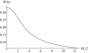
Figure 1: The window function $W(k)$ of (25).

Alternately, we note that $W(k)\geq 0$ and $E_{M}(k)\geq 0$. Then a constraint such as

$$\langle B_{\rm line}^{2}\rangle=\int_{0}^{\infty}\frac{dk}{k}\,W(k)kE_{M}(k)<B_{*}^{2}$$ (26)

means that the integral over every logarithmic interval also satisfies the constraint. Then we can write the constraint as,

$$B_{\lambda}^{2}=2kE_{M}(k)\lesssim\frac{2B_{*}^{2}}{W(k)}$$ (27)

Broadly speaking, current observations place upper bounds on the cosmological magnetic field strength $B_{\lambda}\lesssim 10^{-9}\,{\rm G}$ (up to ${\cal O}(1)$ factors) for $\lambda\sim 100\,{\rm Mpc}-1\,{\rm Gpc}$, while blazar cascade observations place lower bounds $B_{\lambda}\gtrsim 3\times 10^{-16}\,{\rm G}$ assuming $\lambda\gtrsim 10\,{\rm kpc}$ Neronov and Vovk (2010); Essey et al. (2011); Finke et al. (2015); Ackermann et al. (2018). We will refine this statement in Sec. IV.4.

Here we will only discuss blazar observations in detail as these appear to have a lot of promise for detecting and measuring the magnetic field strength and also the magnetic helicity. We will also briefly mention a recent promising proposal based on the effect of magnetic fields on cosmological recombination (see Sec. II.2.2).

II.1 Electromagnetic cascades from blazars

The idea underlying the use of blazars to detect intergalactic magnetic fields is illustrated in Fig. 2 Nikishov (1961); Gould and Schréder (1966); d’ Avezac et al. (2007).

Active galactic nuclei jets that are approximately pointed in our direction are called blazars. The jets have intrinsic opening angles $\sim 1^{\circ}$ Pushkarev et al. (2017) and they can emit very high energy gamma rays, including in the TeV energy range. There are 3 legs in the TeV photon’s journey from the blazar to Earth as we now describe.

In the first leg of its journey, the TeV photon can encounter a photon of the “extra-galactic background light” (EBL). The EBL is due to various sources of infrared photons in the universe, such as stars and active galactic nuclei (AGNs). The EBL spectrum is not known with certainty but it is modeled based on a variety of observations (see Durrer and Neronov (2013) for a summary). The EBL contains photons in the ultraviolet and optical, $0.1-10\,{\rm eV}$. This is important because the TeV photon from the blazar can then scatter off an EBL photon and the center of momentum energy will be above threshold to produce an electron-positron ($e^{+}e^{-}$) pair. The distance that a TeV photon can travel before pair producing off the EBL is Neronov and Semikoz (2009); Durrer and Neronov (2013),

$$D(E)\sim\frac{80~{}{\rm Mpc}}{(1+z_{s})^{2}}\left(\frac{10~{}{\rm TeV}}{E}\right).$$ (28)

up to EBL model-dependent numerical factors; $z_{s}$ is the redshift of the source.

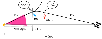
Figure 2: The three legs of the TeV photon’s journey from the blazar to the observer in the presence of an inter-galactic magnetic field. The first TeV leg is terminated by pair production off an EBL photon, the second leg is in the form of lepton pairs and is terminated by an inverse Compton (I.C.) scattering event. The final GeV photon leg then propagates to the detector, perhaps onboard a satellite. Note that the second leg length scale of $\sim{\rm kpc}$ shown in the drawing is the mean free path of the electron and not the cooling distance which is $\sim 300\,{\rm kpc}$. In any case, the second leg of the journey is tiny compared to the first leg $\sim 100~{}{\rm Mpc}$ and the third leg $\sim 1~{}{\rm Gpc}$. Only the second leg probes the inter-galactic magnetic field.

The second leg of the journey is the propagation of the $e^{+}e^{-}$that carry the original TeV energy. Kinematics tells us that the angle the electron and positron make with the forward direction is $\sim m_{e}/{\rm TeV}\sim 10^{-6}$ where $m_{e}=0.5\,{\rm MeV}$ is the mass of the electron.

Coming to the third leg of the journey, electrons and positrons can only propagate a short distance before encountering CMB photons – the most abundant photons in the universe with energy $\sim 10^{-4}\,{\rm eV}$ and number density $n_{\rm CMB}\sim 500/{\rm cm}^{3}$. The mean free path is $l\sim 1/(n_{\rm CMB}\sigma_{T})\sim{\rm kpc}$ where $\sigma_{T}=6.6\times 10^{-25}\,{\rm cm}^{2}$ is the Thomson cross-section.

Inverse-Compton scattering of the electron with a CMB photon BLUMENTHAL and GOULD (1970), up-scatters the CMB photon to energy,

$$E^{\prime}_{\gamma}=\frac{4}{3}E_{\rm CMB}\frac{E_{e}^{2}}{m_{e}^{2}}.$$ (29)

The resulting $\sim{\rm GeV}$ gamma ray has momentum within an angle $m_{e}/E_{e}\sim 10^{-6}$ of the forward direction. In this process, the TeV electron loses a tiny fraction of its energy. Hence up-scattering can continue to produce an “electromagnetic cascade” of GeV photons until the electron loses most of its energy, which occurs over a distance Neronov and Semikoz (2009)

$$D_{\rm IC}=\frac{3m_{e}^{2}}{4\sigma_{T}\rho_{\rm CMB}E_{e}}\approx 300\left(\frac{1\,{\rm TeV}}{E_{e}}\right)\,{\rm kpc}$$ (30)

with $\rho_{\rm CMB}=0.25\,{\rm eV}/{\rm cm}^{3}$ being the energy density in the CMB. Note that $300\,{\rm kpc}$ is much shorter than the $\sim 100\,{\rm Mpc}$ distance from the source as well as the $\sim\,{\rm Gpc}$ distance to the observer. It is only within this short distance that the propagation is via charged particles that are sensitive to the presence of a magnetic field. The resulting GeV gamma rays also have momenta within an angle $\sim 10^{-6}$ with the forward direction. Since the up-scattered CMB photons now have GeV energies and are propagating very close to the forward direction, they arrive to the observer as GeV gamma rays. Thus TeV blazars should be observed to have GeV halos, also called “pair halos”, and the blazar spectrum should show an excess of GeV photons due to the cascade.

How do inter-galactic magnetic fields affect the electromagnetic cascade? The trajectories of $e^{+}e^{-}$  in the second leg of the journey get bent due to the Lorentz force and, if the field is strong enough, the final GeV photons are no longer directed towards the observer and the GeV halo is not seen. Non-observation of the halo can lead to lower bounds on the strength of the inter-galactic magnetic field (see Sec. II.1.2); observations of a dispersed halo can lead to measurements of the magnetic field strength (see Sec. II.1.3). An important caveat to this observational technique is that there be no other mechanism besides magnetic fields by which the $e^{+}e^{-}$  and the GeV photons can be dispersed (see Sec. II.1.1).

To determine the spread of the halo due to a magnetic field we consider two limiting cases. First, if the magnetic field is uniform on the scale of the Larmor radius, $R_{L}=E_{e}/eB\sim 100\,{\rm Mpc}$ for $E_{e}\sim 1\,{\rm TeV}$ and $B\sim 10^{-17}\,{\rm G}$, then the bending angle is $\sim D_{\rm IC}/R_{L}\sim 10^{-3}=0.1^{\circ}$. The other case, of more relevance to causal generation of magnetic fields, is if the magnetic field is isotropic on the scale of the Larmor radius, then the lepton trajectory is a random walk and the bending angle is Neronov and Semikoz (2009),

$$\delta \approx \frac{\sqrt{D_{\rm IC}\lambda_{B}}}{R_{L}}$$ (31)

$$\sim 10^{-4}\left(\frac{\lambda_{B}}{1\,{\rm kpc}}\right)^{1/2}\left(\frac{B}{10^{-17}\,{\rm G}}\right)\left(\frac{1\,{\rm TeV}}{E_{e}}\right)$$

where $\lambda_{B}$ is the coherence scale of the magnetic field. For $B\gtrsim 10^{-13}\,{\rm G}$ on kpc scales we find $\delta\sim 1$ and the small angle approximation is not valid. We expect the halo to be very dispersed for such values of the field strength.

A novelty of using blazars to detect magnetic fields is that the technique is immune to confounding effects at the blazar or in the Milky Way. The $e^{+}e^{-}$  only probe the magnetic field $\sim 100~{}{\rm Mpc}$ away from the blazar. Hence this probe is insensitive to the processes occurring in the blazar. And since the signal arrives at Earth in the form of GeV gamma rays, the Milky Way magnetic field does not play any role. This is a tremendous advantage of using blazar halos as an observational tool.

II.1.1 Plasma instability?

The interpretation of missing blazar halos as being due to inter-galactic magnetic fields has been debated in Refs. Broderick et al. (2012a); Schlickeiser et al. (2012, 2013); Miniati and Elyiv (2013); Yan et al. (2018); Pfrommer et al. (2013); Chang et al. (2014); Supsar and Schlickeiser (2014); Chang et al. (2016); Broderick et al. (2016a); Shalaby et al. (2017); Tiede et al. (2017a, b); Broderick et al. (2018); Shalaby et al. (2018); Batista et al. (2019); Shalaby et al. (2020). The question is if the $e^{+}e^{-}$  beam can excite a plasma instability and lose energy faster than the rate at which IC scattering cools the beam. If so, the energy in the $e^{+}e^{-}$  beam would go into heating the cosmological medium, not into GeV photons.

The basic physics of the main instability is illustrated in Fig. 3. (Other instabilities, such as the Weibel instability, grow more slowly.) The relevant comparison is the timescale for the growth of the instability versus the cooling time due to IC scattering. In Ref. Broderick et al. (2012a), the timescale of instability growth is estimated to be $10^{3}-10^{5}~{}{\rm yrs}$, whereas the IC cooling distance estimated at $\sim 300\,{\rm kpc}$ in (30) equates to an IC cooling time of $10^{6}\,{\rm yrs}$. Then the instability growth rate is faster and will be the main cause of the lepton beam dispersal. However, the matter is still under debate. Objections have been raised based on simulation results, backreaction on the background, non-linear effects, and parameters such as the intrinsic spectrum of the blazar, density and temperature of the inter-galactic medium, and the luminosity of the beam (e.g. Batista et al. (2019)).

While the relevance of plasma instabilities is still under investigation, observations may be able to directly settle the issue – if a dilute GeV halo is detected around TeV blazars then clearly plasma instabilities are not playing a role since these dissipate the energy of the $e^{+}e^{-}$beam to heat and not to GeV photons (see Sec. II.1.3 below).

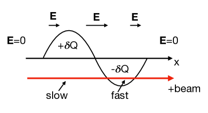
Figure 3: The drawing shows the basic physics underlying the plasma instability. A beam of charged particles (red arrow) is injected into a neutral plasma. The plasma may have perturbations in the charge density distribution so that there is an excess charge $+\delta Q$ at one location and $-\delta Q$ somewhere else, and these are taken to be a fixed background for illustrative purposes. (In general, charge perturbations would be expanded in modes.) The electric field ${\bf E}$ due to this perturbation is depicted above and the key feature is that it points to the right everywhere (the $\pm\delta Q$ charge distribution is like a charged capacitor) and the electric field is nearly zero away from the perturbed region. Positively charged particles in the beam enter from the left and are moving with their (“slow”) initial velocity as they enter the $+\delta Q$ region where they get accelerated to the right by the electric field, and then they move faster through the $-\delta Q$ region. Thus they spend more time in the $+\delta Q$ region than in the $-\delta Q$ region and effectively enhance the perturbation. Similarly, negative charges in the beam spend more time in the $-\delta Q$ region and also enhance the perturbation. Other charged particles in the beam will effectively experience a larger charge perturbation and in this way the perturbation can grow. This is the basic idea of the instability. In Ref. Broderick et al. (2012b) it is argued that the instability grows fastest when the beam is obliquely incident on the perturbation wavevector.

II.1.2 Evidence from blazar spectra

An analysis of blazar spectra was performed in Ref. Neronov and Vovk (2010) and obtained a lower bound $\sim 10^{-16}~{}{\rm G}$ on the inter-galactic field assuming homogeneity on 1 Mpc scales. Since then a number of other groups have performed similar analyses, though the lower bounds have varied from $\sim 10^{-19}~{}{\rm G}$ to $\sim 10^{-17}~{}{\rm G}$ depending on the details of the analysis Neronov and Vovk (2010); Essey et al. (2011); Finke et al. (2015); Ackermann et al. (2018). The analysis of Arlen et al. (2014) concludes that the data is consistent with zero magnetic field but may have adopted an unrealistic model for the intrinsic spectra of blazars and the EBL Durrer and Caprini (2003). Fig. 4 shows the main plot from Ref. Neronov and Vovk (2010) for the spectra from three blazars and the analysis.

The absence of GeV halos can be explained by magnetic fields that are stronger than $10^{-16}\,{\rm G}$ on $\sim{\rm Mpc}$ scales as in Neronov and Vovk (2010) but other combinations of strength and coherence scale are also possible. For example, magnetic fields weaker than $10^{-16}\,{\rm G}$ on $\sim{\rm Mpc}$ scales but stronger on smaller scales, e.g. $10^{-14}\,{\rm G}$ on $\sim{\rm kpc}$ scales, can equally well cause sufficient deflection of the lepton pairs and dilute the GeV halos. In other words, the lower bound is on an appropriately weighted integral of the power spectrum $E_{M}(k)$ and the quoted bound of “$10^{-16}\,{\rm G}$ on $\sim{\rm Mpc}$ scales” should not be taken too literally.

The important point of this analysis is that there exists a lower bound on the magnetic field strength, with the most recent analysis by the Fermi collaboration Ackermann et al. (2018), even if the numerical value of the lower bound is model-dependent. The only known alternative explanation for the spectral signature is the plasma instability discussed in Sec. II.1.1. Yet it may be possible to distinguish between the two scenarios by direct observations of the halo as we now discuss.

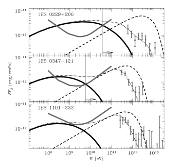
Figure 4: Data points from HESS observations for three blazars together with a model of the EBL are used to deduce the primary source spectrum (dashed curves), the cascade contribution (solid curve) and the net processed spectrum (dotted curves). Constraints imposed by Fermi observations (grey concave solid curves) are however lower than the predicted spectrum at GeV energies. The deficit of GeV gamma rays provides lower bounds on the strength of the inter-galactic magnetic field. [Plot from Ref. Neronov and Vovk (2010).]

II.1.3 Detection of the halo

The pair halo around a single blazar may be too diffuse to be seen with current observations. The strategy employed in Refs. Ando and Kusenko (2010); Chen et al. (2015a) is to stack images of several different blazars to get a larger photon count and then look for an excess of pair halo GeV photons. To decide if there is an excess one compares the stacked results for TeV sources (BL Lacs) with an identical stacked analysis for similar sources but for which pair halos are not to be expected (Flat Spectrum Radio Quasars or FSRQs). In Fig. 5 we show the results from Ref. Chen et al. (2015a).

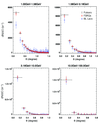
Figure 5: Data points show the count of GeV photons in various energy bins versus angular distance from 24 stacked sources for 3 different classes of sources: Pulsars (black bar), FSRQs (red bar with circle), and the TeV-luminous BL Lacs (blue bar with cross). The pulsar and FSRQ counts agree with each other but there is an excess count from the BL Lacs at large angular distances with $\sim 3.5\sigma$ significance in the lowest energy bin (top left plot) as would be expected if there was a pair halo around BL Lacs. [Plot from Ref. Chen et al. (2015a).]

The claimed detection of pair halos is not universally accepted. The earliest claimed evidence for pair halos in a stacked analysis Ando and Kusenko (2010) was argued to be due to an instrumental effect Neronov, A. et al. (2011). Other analyses by the Fermi collaboration Ackermann et al. (2018) and the VERITAS collaboration Archambault et al. (2017) did not corroborate evidence for pair halos. Further data will help to clarify the situation; improved analysis techniques, such as the idea to use radio observations to align blazar jet directions prior to stacking can enhance the sensitivity of the stacking method Tiede et al. (2017c); Chen et al. (2018).

II.1.4 Halo morphology

Several groups have studied the shape and structure of pair halos Elyiv et al. (2009); Alves Batista et al. (2016); Alves Batista and Saveliev (2018); Long and Vachaspati (2015); Duplessis and Vachaspati (2017); Broderick et al. (2016b); Fitoussi et al. (2017); Kachelriess and Martinez (2020). A full simulation is complicated, especially in a stochastic magnetic field, but some features of the effect of a magnetic field on the halo are simple to understand based on the structure of the surface where pair production can occur Duplessis and Vachaspati (2017).

Consider the simple setup where the blazar jet points directly at the observer and there is no magnetic field ($B=0$). Then, assuming an axially symmetric jet, the halo will also be axially symmetric and will appear as a disk to the observer. Next let us introduce a uniform magnetic field that is orthogonal to the line of sight. This breaks the axial symmetry because charges bend by different amounts depending on their direction of propagation and the sign of the charge Long and Vachaspati (2015). Then the halo stretches out in the two directions orthogonal to the line of sight and to the magnetic field direction. The higher energy charged particles are bent less by the magnetic fields and the gamma ray cascade they produce tend to cluster close to the line of sight, while the lower energy gamma rays lie further away from the line of sight. This gives the halo a “bow-tie” structure Broderick et al. (2016b), at least for magnetic fields that are highly coherent, as illustrated in Fig. 6. The two sides of the bow tie also have an interesting origin. When the TeV gamma rays pair produce, the electrons will bend one way due to the Lorentz force exerted by the magnetic field while the positrons will bend in the opposite way. One side of the bow-tie is due to photons that have been up-scattered by electrons, while the other side of the bow-tie is due to up-scattering by positrons. If the blazar jet is not directly pointed at the observer, one side of the bow-tie will be less prominent than the other as in Fig. 7. If the magnetic field is helical, the bow-tie shape also gets twisted, either in a clockwise or in a counter-clockwise direction depending on the sign of the helicity, also seen in Fig. 7). Features of the halo may be understood in terms of a “particle production surface” as in Fig. 8.

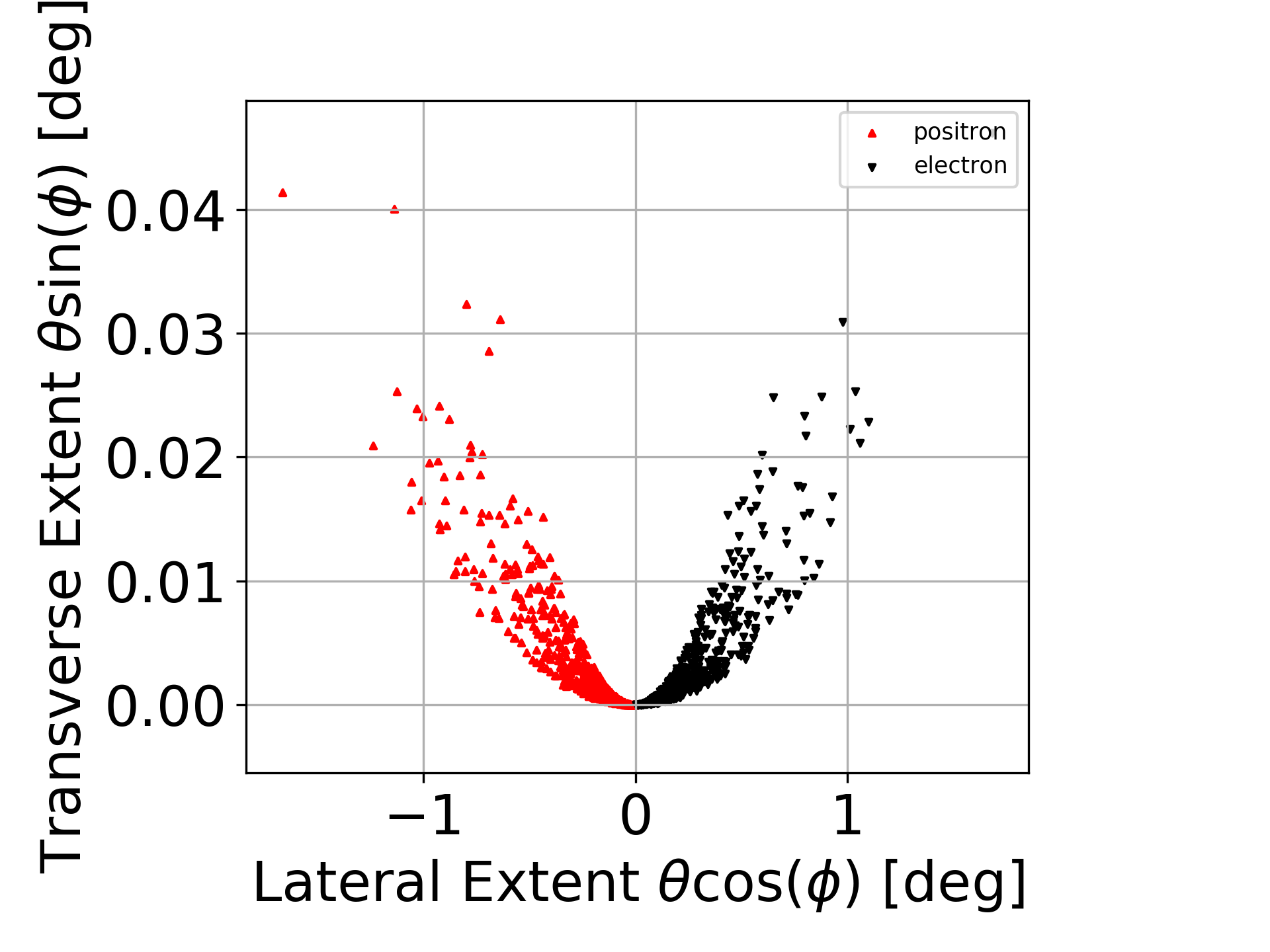
Figure 6: The halo for a magnetic field that is at a $45^{\circ}$ angle to the line of sight to a blazar whose jet is pointed to the observer. (Photon energy information is not shown.) If the magnetic field was chosen to be orthogonal to the line of sight, the two branches would have been straight, giving a bow-tie shape. The red dots correspond to photons that have been up-scattered by positrons and the black dots due to up-scattering by electrons. If the blazar jet axis is misaligned with the line of sight, the bow-tie will not be symmetrical.

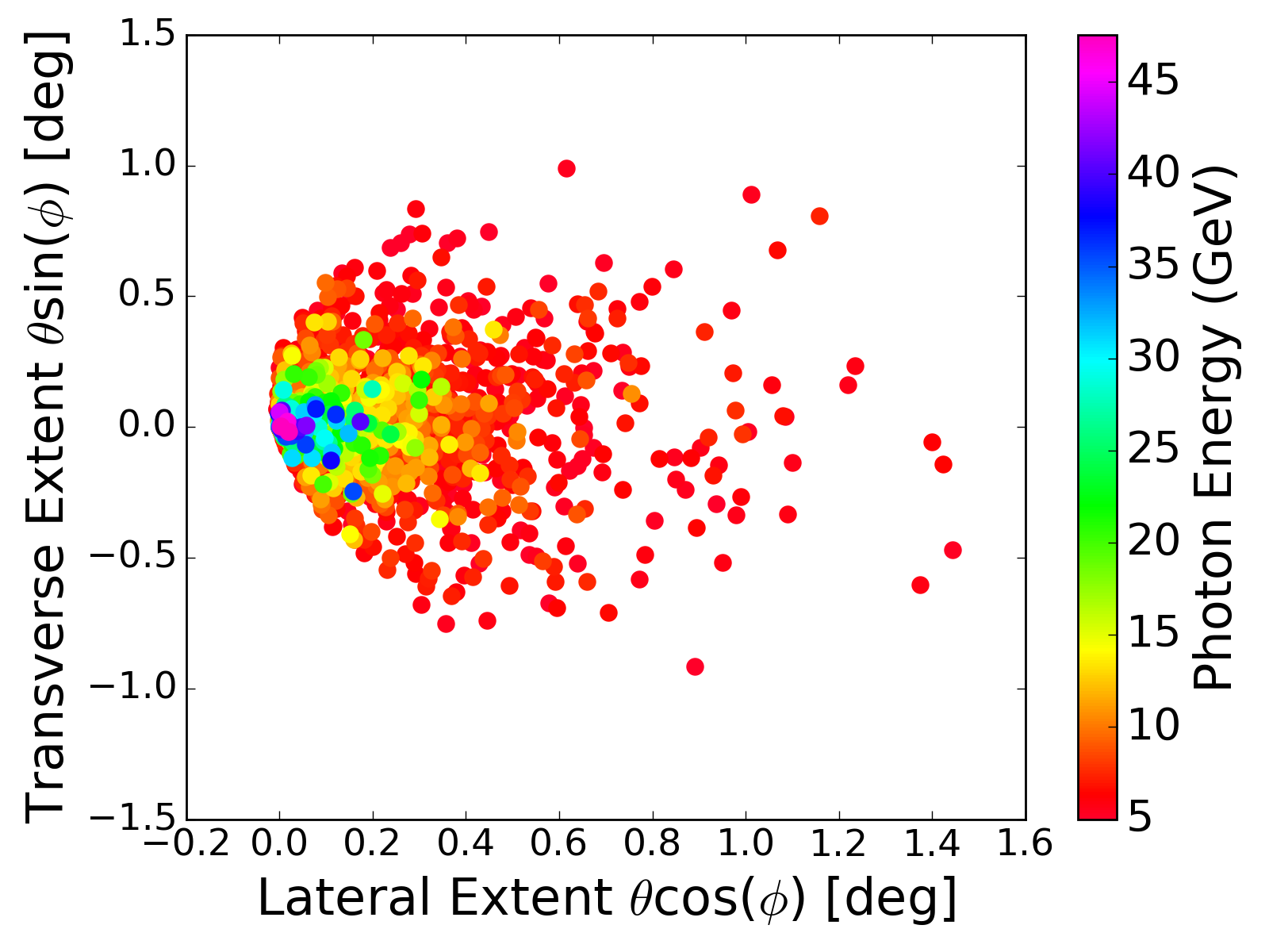
Figure 7: The halo for a helical field and a blazar jet that is misaligned with the line of sight. (Details may be found in Ref. Duplessis and Vachaspati (2017).) The misalignment in this case eliminates one of the lepton branches of the halo. The different color dots represent photons of various energies as shown on the bar on the right and the energetic photons lie closer to the line of sight. The helicity of the magnetic field provides a twist to the distribution of photons of different energies in the halo.

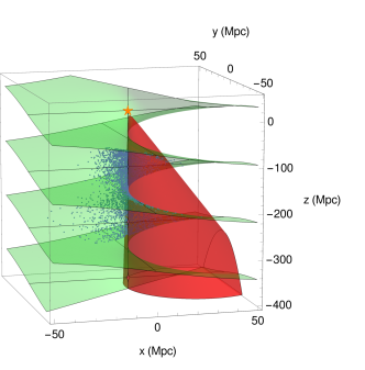
Figure 8: The TeV photons from the blazar (yellow star) travel a certain distance, pair produce, up-scatter CMB photons that reach the observer. This process maps out a spatial surface called the “particle production surface” (shown in green) that depends on the inter-galactic magnetic field, such that only pair creation events on the surface can potentially be observed. For helical magnetic fields, the surface has a spiral structure. The blue dots represent potential pair creation events that can be observed though an actual jet (shown as the red cone) may not activate all the possible observable pair creation events Duplessis and Vachaspati (2017).

II.1.5 Search for magnetic helicity

The twisting of the halo provides a handle for the detection of inter-galactic magnetic fields and their helicity. This might seem like a “second order effect” – we first need to detect magnetic fields which is hard and then its helicity which seems harder. However, since helicity is a parity odd feature, its signatures are protected from confusion with foregrounds and most other sources of noise as those are generally parity even. There is an additional high-stakes reason for seeking magnetic helicity as it would be direct evidence for the violation of fundamental symmetries (P, CP) in particle physics and cosmology. On top of this, a detection of magnetic helicity will also resolve the ambiguity between the magnetic field interpretation of missing pair halos and the interpretation in terms of plasma instabilities. Another motivation to search for magnetic helicity is that MHD evolution, to be discussed later, shows that helicity is an essential feature if causally generated magnetic fields are to survive on large length scales. If magnetic fields are discovered but they are not helical, it would indicate an acausal generation mechanism or an astrophysical mechanism in the very recent universe.

The detection of magnetic helicity using parity odd correlators of the CMB was discussed in Ref. Caprini et al. (2004). Techniques for detecting magnetic helicity using blazar data were first discussed in Tashiro and Vachaspati (2013, 2015) following ideas in Kahniashvili and Vachaspati (2006). If ${\hat{l}}$ denotes the line of sight to a blazar, the twisting of a particular halo can be measured by ${\hat{n}}_{1}\times{\hat{n}}_{2}\cdot{\hat{l}}$ where ${\hat{n}}_{a}$ refers to the arrival directions of gamma rays of energy $E_{a}$, and we order the energies so that $E_{1}<E_{2}$. Hence the twisting of a single blazar halo can be measured by computing

$$Q(R)=\langle{\hat{n}}_{1}\times{\hat{n}}_{2}\cdot{\hat{l}}\rangle_{R}$$ (32)

where the angular brackets refer to an average over all photons around the blazar out to an angular distance of $R$.

In fact, the line of sight direction nearly coincides with the direction of propagation of the highest energy gamma rays. So the line of sight direction can be approximated by ${\hat{n}}_{3}$ for a photon with very high energy $E_{3}$ and the twisting can be measured by calculating ${\hat{n}}_{1}\times{\hat{n}}_{2}\cdot{\hat{n}}_{3}$ where the energies are ordered: $E_{1}<E_{2}<E_{3}$. Since now there is no reference to an observed blazar, this quantity can be calculated over the entire sky with sums over all photons with energies $E_{1}$, $E_{2}$ and $E_{3}$. This will tell us if there is an overall handedness in the gamma ray sky. This leads to the statistic $Q$ for measuring magnetic helicity over the entire sky whether or not blazars are identified,

$$Q({\hat{n}}_{1},{\hat{n}}_{2},{\hat{n}}_{3};R)=\frac{1}{N}\sum_{\{n_{a}\}}{\hat{n}}_{1}\times{\hat{n}}_{2}\cdot{\hat{n}}_{3}$$ (33)

where $N$ is the total number of terms in the sum. Since $Q$ is parity odd, it is no surprise that it is proportional to the helical part of the magnetic field correlator, $M_{H}$, in (2). In the idealized case of no backgrounds, small deflection angles, and large angular regions (to capture all GeV photons) Tashiro and Vachaspati (2015),

$$Q(E_{1},E_{2},E_{3};R\to\pi/2)\propto r\,M_{H}(r)$$ (34)

where the distance $r$ is related to the energies $E_{1}$ and $E_{2}$. By considering different photon energies $E_{1}$ and $E_{2}$, the statistics $Q$ can probe the helical spectrum at different spatial separations and, in principle, we can recover the entire helical power spectrum. As we shall see in Sec. IV, causally generated magnetic fields are expected to be maximally helical, in which case the helical power spectrum is related to the power spectrum, $E_{M}(k)$. Thus we can recover the entire correlation function for the magnetic field from the $Q$ statistics.

To actually compute $Q$ from data requires some more refinements as there are confounding gamma rays that originate in the Milky Way and in other known sources. Using 11 years of Fermi Observatory data and only including the highest energy gamma rays ($E_{3}=50-60\,{\rm GeV}$) at galactic latitudes above $80^{\circ}$, and for various combinations of $E_{1}$ and $E_{2}$ leads to the $Q(R)$ plots shown in Fig. 9. The error bars in the plot are statistical. The question is if the non-zero values of $Q$ are significant. This requires a careful analysis such as in Refs. Asplund et al. (2020); Kachelriess and Martinez (2020) with the conclusion that the plots of $Q$ are consistent with vanishing helicity.

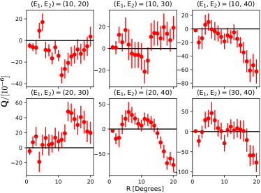
Figure 9: The $Q/10^{-6}$ statistic plotted vs. the angular size $R$ for various values of $(E_{1},E_{2})$ and for $E_{3}>50\,{\rm GeV}$. These plots are for 11 years of Fermi data, following the scheme in Tashiro et al. (2014); Chen et al. (2015b). [Plot by Teerthal Patel, unpublished.]

At this point in time the detection of magnetic helicity via the twisting of halos is still not conclusive but, given the compelling motivations for pursuing helicity, it is important to develop new strategies. Already a refinement of $Q$ has been proposed in Duplessis and Vachaspati (2017) that limits the sum in (33) to just one branch of the bow-tie (to avoid terms that involve cross products of GeV photon direction vectors from electron up-scatterings and those from positron up-scatterings). In relatively simple simulations the refined $Q$ is seen to have greater sensitivity to magnetic helicity Duplessis and Vachaspati (2017) . On the observational front, in future we expect more gamma ray data will be available around individual blazars on which to apply the $Q$ statistic. Or perhaps the evaluation of $Q$ on stacked data will be more conclusive. Here we would need to ensure that the halo bow ties are aligned prior to stacking as mentioned in Sec. II.1.3.

II.1.6 Pair echoes

If a transient source such as a GRB emits TeV photons, these photons too will undergo a cascade and produce GeV photons as described above. In the presence of inter-galactic magnetic fields, the GeV photons will be delayed because the path length after bending is longer than the line of sight path length (see Fig. 2) and lead to a “pair echo”. Stronger magnetic fields will cause greater time delays in the arrival of halo photons of a given energy. Therefore a measured time delay can lead to a measurement of the magnetic field strength, while non-observation of an echo can lead to a lower bound Plaga (1995); Taylor et al. (2011); Veres et al. (2017). Ref. Taylor et al. (2011) finds a bound $\gtrsim 10^{-17}\,{\rm G}$, while Veres et al. (2017); Wang et al. (2020) obtain $\gtrsim 10^{-19}\,{\rm G}$. The analysis of Wang et al. (2020) has been criticized in Dzhatdoev et al. (2020).

II.2 Observations at high redshift

II.2.1 Magnetic fields in high redshift galaxies

The Milky Way has magnetic field strength $\sim 10^{-6}\,{\rm G}$, rotational velocity $\sim 200\,{\rm km/s}$, and disk radius $\sim 30\,{\rm kpc}$ and baryon density $\rho_{\rm gal}\approx 10^{-24}\,{\rm gm/cm^{3}}$. If we assume flux freezing during gravitational collapse of a proto-galaxy, the magnetic field strength increases in this process by a factor $(\rho_{\rm gal}/\rho_{b})^{2/3}\sim 10^{5}$ where $\rho_{b}\sim 10^{-31}\,{\rm gm/cm^{3}}$ is the average cosmological baryon density. Therefore $\sim 10^{-11}\,{\rm G}$ cosmological magnetic fields can give rise to the galactic field strength $\sim\mu{\rm G}$ simply by gravitational compression.

Assuming that the observed galactic field of $\sim 1\,\mu{\rm G}$ is due to dynamo amplification of a seed field in addition to gravitational compression, and each full rotation of the galaxy amplifies the field strength by an e-fold (“a maximally efficient dynamo”), the seed field required to explain the Milky Way magnetic field is $\sim e^{-40}10^{-5}10^{-6}~{}{\rm G}$ or about $10^{-29}~{}{\rm G}$, since the Milky Way is estimated to have made $~{}40$ complete revolutions. Such a tiny seed field may possibly have arisen from a Biermann battery mechanism assuming certain dynamics during galaxy formation Subramanian et al. (1994); Kulsrud et al. (1997).

A difficulty with the large-scale dynamo is that micro Gauss fields have also been observed in galaxies at a redshift $\sim 2$ Bernet et al. (2008); Kronberg et al. (2008) when the universe was only $\sim 1/5$ of its present age. Such galaxies would at most have gone through $\sim 40/5=8$ revolutions and the maximum dynamo amplification would only be by a factor $\sim 10^{3}$. Then the seed field would need to be around a $10^{-14}\,{\rm G}$ which is much harder to arrange by astrophysics alone. An alternate scenario based on a turbulent dynamo is discussed in Kulsrud et al. (1997).

II.2.2 Magnetic fields and cosmological recombination

CMB anisotropies generally impose constraints on cosmological magnetic fields at the nano Gauss level. To see that this is reasonable, consider that CMB observables mostly depend on adiabatic density fluctuations in the primordial plasma with $\delta\rho/\rho\sim 10^{-5}$. As estimated in Sec. I.2, the energy density in micro Gauss magnetic fields is of the same order as that in CMB photons today and so nano Gauss magnetic fields can cause density fluctuations on the order of $10^{-6}$. Stronger magnetic fields can start interfering with the successful predictions of adiabatic density fluctuations. This shows very roughly that CMB observations can be expected to lead to constraints on magnetic fields at the nano Gauss level.

As discussed above, most cosmological observations are sensitive to large-scale magnetic fields but small-scale, say kpc, magnetic fields remain weakly constrained. Since causally generated magnetic fields are peaked on small length scales, it is important to find ways to observe and constrain them. The CMB may be used to constrain small-scale fields, not by the large scale anisotropies, instead by using spectral observations (departures from the blackbody spectrum). The effect of small-scale magnetic fields on spectral distortions of the CMB have been considered in Refs. Jedamzik et al. (2000); Kunze and Komatsu (2015); Wagstaff and Banerjee (2015) and generally also lead to nano Gauss constraints on kpc-Mpc scales.

Recently another effect of magnetic fields on recombination and the CMB has been discussed by Jedamzik and collaborators Jedamzik and Abel (2013); Jedamzik and Saveliev (2019); Jedamzik and Pogosian (2020). The basic idea is that the MHD equation for the plasma flow contains the Lorentz force term $\propto{\bf B}\times(\nabla\times{\bf B})$ (see (65)). The stochastic magnetic field will therefore create stochastic density fluctuations in the baryon fluid density Jedamzik and Abel (2013); Jedamzik and Saveliev (2019) that depend mainly on the magnetic field power spectrum on the smallest length scales. The Hydrogen recombination rate is proportional to the square of the baryon density and since the average of the square, $\langle n_{b}^{2}\rangle$, is always larger than the square of the average, $\langle n_{b}\rangle^{2}$, baryonic inhomogeneities lead to faster recombination overall and the sound horizon at recombination, $r_{s}$, is smaller due to the magnetic field. Temperature fluctuation correlations of the CMB are measured as a function of the angular separation of points on the sky and the dominant peak in the spectrum is at an angle, $\theta=r_{s}/l\approx 1^{\circ}$ where $l$ is the distance to the surface of recombination. Hence a smaller sound horizon implies that $l$ is also smaller. The Hubble constant $H_{0}$ enters the expressions for both $r_{s}$ and $l$ but the dependence of $l$ on $H_{0}$ is stronger Pogosian et al. (2020). Since $l$ decreases with increasing $H_{0}$ while $r_{s}$ stays approximately constant, we need a larger $H_{0}$ to keep $\theta\approx 1^{\circ}$ in the presence of magnetic fields. If we do not take the magnetic field into account, CMB measurements will give an anomalously low value of the Hubble constant that will differ from $H_{0}$ measurements made at lower redshifts. In this way, primordial magnetic fields of strength $\sim 0.1\,{\rm nG}$ on kpc scales Jedamzik and Pogosian (2020) can alleviate some of the current tension in the supernovae (nearby) measurements of the Hubble constant, $H_{0}=73.5\pm 1.4~{}{\rm km/s/Mpc}$ Reid et al. (2019), and the (distant) measurements using the CMB that so far have been giving $H_{0}=67.37\pm 0.54~{}{\rm km/s/Mpc}$ Aghanim et al. (2018). Such magnetic fields would comfortably satisfy other existing constraints especially if the spectrum is peaked on short scales like that of causally generated fields. Furthermore, the field strength is in the range where it can directly source observed galactic and cluster magnetic fields with minimal dynamo processing and would explain the observation of magnetic fields in high redshift galaxies.

Although still young, this idea is exciting not only because it potentially resolves a crisis in cosmological observations (the “Hubble tension”) but also because it would be the earliest observational signature of cosmological magnetic fields. It would, by itself, point to an early universe generation mechanism of magnetic fields and indicate new particle physics and cosmology as we discuss in Sec. III.

III Production of magnetic fields in the early universe

Several ideas for the generation of magnetic fields in the early universe have been proposed based on particular epochs in cosmology, such as inflation, the electroweak phase transition, the QCD phase transition, and recombination. Here I will focus on magnetic fields generated at the electroweak phase transition and will only make brief remarks on the other possibilities in Sec. III.2.

III.1 Magnetic fields from the electroweak phase transition

III.1.1 Defining the electromagnetic field strength

The electroweak model contains four gauge fields corresponding to the three generators of the “weak” $SU(2)$ and one generator of hypercharge $U(1)_{Y}$. The $SU(2)$ gauge fields are usually denoted by $W_{\mu}^{a}$ ($a=1,2,3$ and $\mu$ is the Lorentz index) and the hypercharge gauge field by $Y_{\mu}$. The vacuum expectation value (VEV) of the $SU(2)$ doublet Higgs field $\Phi$, breaks the electroweak $SU(2)\times U(1)_{Y}$ symmetry to the electromagnetic $U(1)_{Q}$. The electromagnetic gauge field, $A_{\mu}$, is a linear combination of the weak and hypercharge gauge fields,

$$A_{\mu}=\sin\theta_{w}{\hat{n}}^{a}W^{a}_{\mu}+\cos\theta_{w}Y_{\mu},$$ (35)

where $\theta_{w}$ is the weak mixing angle ($\sin^{2}\theta_{w}\approx 0.23$),

$${\hat{n}}^{a}\equiv-\frac{\Phi^{\dagger}\sigma^{a}\Phi}{\Phi^{\dagger}\Phi}$$ (36)

and $\sigma^{a}$ are the Pauli spin matrices

$$\sigma^{1}=\begin{pmatrix}0&1\\ 1&0\end{pmatrix},\ \ \sigma^{2}=\begin{pmatrix}0&-i\\ i&0\end{pmatrix},\ \ \sigma^{3}=\begin{pmatrix}1&0\\ 0&-1\end{pmatrix}$$ (37)

The vector ${\hat{n}}^{a}$ is ill-defined at locations where $\Phi=0$. These points may correspond to locations of magnetic monopoles and electroweak strings. However, at late times $\Phi$ relaxes to the true vacuum with $|\Phi|=\eta\approx 174\,{\rm GeV}$ everywhere and then $n^{a}$ is globally defined.

One might think that the electromagnetic field strength, $A_{\mu\nu}$, equivalently the electric and magnetic fields, should be defined in the usual way

$$A_{\mu\nu}\stackrel{{\scriptstyle?}}{{=}}\sin\theta_{w}{\hat{n}}^{a}W^{a}_{\mu\nu}+\cos\theta_{w}Y_{\mu\nu}$$ (38)

but this definition has the difficulty that the right-hand side does not correspond to the Maxellian $\partial_{\mu}A_{\nu}-\partial_{\nu}A_{\mu}$ for two reasons: first, the derivatives $\partial_{\mu}A_{\nu}$ will also in general act on ${\hat{n}}^{a}$; second, $W^{a}_{\mu\nu}$ has terms that are quadratic in the gauge fields $W^{a}_{\mu}$ and these are absent in $\partial_{\mu}A_{\nu}-\partial_{\nu}A_{\mu}$ as calculated from the definition in (35). The former difficulty can be avoided in the broken phase where $\Phi$ can be gauge transformed to a constant (the “unitary gauge”) but we are still stuck with the second difficulty. We would like to eliminate the quadratic term in $W^{a}_{\mu}$ in (38) while obtaining the Maxwellian field strength in the unitary gauge (in which $\Phi$ is uniform). Following ’t Hooft’s definition for an SO(3) model ’t Hooft (1974), a resolution is to define Vachaspati (1991)

$$A_{\mu\nu} = \sin\theta_{w}{\hat{n}}^{a}W^{a}_{\mu\nu}+\cos\theta_{w}Y_{\mu\nu}$$ (39)

$$-i\frac{2\sin\theta_{w}}{g\eta^{2}}(D_{\mu}\Phi^{\dagger}D_{\nu}\Phi-D_{\nu}\Phi^{\dagger}D_{\mu}\Phi)$$

in the true vacuum where $\Phi^{\dagger}\Phi=\eta^{2}$. A little algebra then shows that

$$A_{\mu\nu} = \partial_{\mu}A_{\nu}-\partial_{\nu}A_{\mu}$$ (40)

$$-i\frac{2\sin\theta_{w}}{g\eta^{2}}(\partial_{\mu}\Phi^{\dagger}\partial_{\nu}\Phi-\partial_{\nu}\Phi^{\dagger}\partial_{\mu}\Phi)$$

Then there can be a non-zero electromagnetic field even if $A_{\mu}=0$ due to gradients of the Higgs field. One could choose to work in unitary gauge and then the usual Maxwellian expression for the electromagnetic field holds. The advantage of not working in unitary gauge is that (i) we can treat $\Phi$ as a dynamical field and it is more straightforward to solve the equations of motion without going to unitary gauge, and (ii) there are monopole-like configurations in the electroweak model Nambu (1977); Achucarro and Vachaspati (2000) that make it cumbersome to go to unitary gauge during the phase transition. These electroweak monopoles are singularities in the vector field ${\hat{n}}^{a}$. An electroweak monopole is not topological because it is connected to an antimonopole by a string made of $Z$ magnetic field. Note that $Z_{\mu}$ is orthogonal to $A_{\mu}$ and is defined by,

$$Z_{\mu}=\cos\theta_{w}{\hat{n}}^{a}W^{a}_{\mu}-\sin\theta_{w}Y_{\mu},$$ (41)

The $Z-$string that confines electroweak monopoles is unrelated to the electromagnetic magnetic field that emanates from the monopole and antimonopole at the ends of the string. The configuration is reminiscent of electrically charged quarks at the end of a gluonic string in QCD.

III.1.2 Generation of magnetic fields: physical arguments

There are several ways to physically understand the generation of magnetic fields during the electroweak phase transition and obtain qualitative results with rough estimates Vachaspati (1991). More quantitative results can be obtained from numerical simulations as described in Sec. III.1.4.

At the electroweak phase transition, the Higgs field $\Phi$ gets a VEV but the orientation of the VEV is undetermined. The only constraint is $\Phi^{\dagger}\Phi=\eta^{2}$. Since $\Phi$ has four real degrees of freedom, the constraint restricts the VEV of $\Phi$ to live on a three sphere that can be parametrized as,

$$\Phi=\eta\begin{pmatrix}\sin\alpha\,e^{i\beta}\\ \cos\alpha\,e^{i\gamma}\end{pmatrix}$$ (42)

where $\alpha\in[0,\pi/2]$, $\beta\in[0,2\pi]$, $\gamma\in[0,2\pi]$ are the (Hopf) angular coordinates on the three-sphere.

Just as in the Kibble argument used in the formation of topological defects Kibble (1976), the Higgs VEV will be different in different spatial domains and $\partial_{\mu}\Phi\neq 0$ in general. Then the last term in (40) will in general not vanish and there is no reason to expect the Maxwell field strength, $\partial_{\mu}A_{\nu}-\partial_{\nu}A_{\mu}$, to compensate the terms arising from the Higgs field. In fact, because of electroweak magnetic monopoles, there are field configurations where compensation is impossible because the divergence of the Maxwell field strength vanishes while that of the scalar Higgs does not. Therefore we expect non-zero magnetic fields after the phase transition.

The connection with topological defects can be taken further Vachaspati (1994). We have already discussed that the divergence of magnetic fields in electroweak theory need not vanish and that there are magnetic monopole configurations in the model. For example, a monopole can have the asymptotic field configuration in (42) with $\alpha=\theta/2$, $\beta=\phi$ and $\gamma=0$, where $\theta$, $\phi$ are spherical angles, and have $\Phi=0$ at their centers Nambu (1977). During the phase transition we can expect that magnetic monopole configurations will be created but that the monopoles and anti-monopoles will quickly annihilate since they are confined by Z-strings that will pull them together. However, a monopole-antimonopole pair (also called a “dumbbell” Nambu (1977)) has a magnetic dipole field and the annihilation of the dumbbell will release the magnetic fields into the ambient plasma. Thus the post-phase transition plasma should be magnetized.

To get an estimate of $E_{M}(k)$ following from the electroweak phase transition, we will first estimate $B_{V,\lambda}$ defined in (17). We start by evaluating the volume averaged magnetic field of (16) using the expression for the magnetic field generated at the EWPT due to Higgs gradients as in (40). Then,

$$({\bf B}_{V})_{i} \sim -i\frac{2\sin\theta_{w}}{g\eta^{2}}\frac{1}{V}\int_{V}d^{3}x\,\epsilon_{ijk}\partial_{j}\Phi^{\dagger}\partial_{k}\Phi$$ (43)

$$\sim -i\frac{2\sin\theta_{w}}{g\eta^{2}}\frac{1}{V}\int_{\partial V}dS^{j}\,\epsilon_{ijk}\Phi^{\dagger}\partial_{k}\Phi$$

where we have performed an integration by parts. The final surface integral can be written in terms of the angles on the three-sphere appearing in (42) under the assumption that $|\Phi|\sim\eta$ on the surface of integration. The Hopf angles are random variables with probability distributions such that every point on the three-sphere is equally probable. Since the volume element in Hopf coordinates is $(1/2)d(\cos(2\alpha))\,d\beta\,d\gamma$, the variables $\cos(2\alpha)$, $\beta$ and $\gamma$ are uniformly distributed over their ranges and take on different values in different spatial domains. The final surface integral can now be estimated by assuming that the Hopf angles are approximately constant in domains of size $\xi$. Then the random elements of the surface integral add up as a random walk and the root-mean-squared value of the integral goes as the square root of the number of domains on the surface, i.e. proportional to $\lambda/\xi$ where $\lambda\sim V^{1/3}$ is the characteristic size of the volume $V$. Therefore

$$B_{V,\lambda}\propto\frac{\lambda}{V}\propto\frac{1}{\lambda^{2}}\propto k^{2}$$ (44)

and from (17),

$$E_{M}(k)\sim\frac{1}{k}B^{2}_{V,\lambda}\sim k^{3}.$$ (45)

Note that this estimate using the surface integral does not assume anything about $|\Phi|$ within the volume of integration and therefore includes the possibility of magnetic monopoles within the volume during the EWPT. A direct estimate of the volume integral in (43) along similar lines would need to assume the absence of magnetic monopoles since these necessarily have $|\Phi|=0$ at their locations.

Two comments about the estimate in (45) are necessary. First, in contrast to our estimate here, the estimate in Vachaspati (1991) used a different definition of the “average magnetic field” that has been criticized in Refs. Enqvist and Olesen (1993); Hindmarsh and Everett (1998). The estimate given here is more useful because it derives the $k$ dependence of the power spectrum $E_{M}(k)$ in an unambiguous way. The crucial point is that the magnetic field is given by surface (not volume) fluctuations (see (43)). Second, Ref. Durrer and Caprini (2003) argues that causality considerations imply that fields should have vanishing correlation functions beyond a certain length scale, and in that case if $E_{M}(k)\propto k^{n}$ then necessarily $n\geq 4$, in contradiction with the $E_{M}\propto k^{3}$ derived above. It is certainly true that if correlations in physical space cutoff sharply, the power spectrum must fall off fast enough for small $k$. However it is questionable if the premise of the argument applies to our situation. There are several physical systems that have non-vanishing field correlators on arbitrarily large distance scales. For example, for a free scalar field $\phi$ at temperature $T$, the field two-point correlator at large separations is (e.g. Sec. 3.1 in Laine and Vuorinen (2016)),

$$\langle\phi({\bf x}+{\bf r})\phi({\bf x})\rangle_{T}\sim\frac{T}{4\pi|{\bf r}|}e^{-m|{{\bf r}}|},\ \ |{\bf r}|\gg T^{-1}$$ (46)

where $m$ is the mass of $\phi$. The correlator is non-vanishing for all $|{\bf r}|$; yet this does not signal a violation of causality.

A similar calculation can be done for the correlation function of magnetic fields in a thermal bath of photons with the result,

$$\langle B_{i}({\bf x}+{\bf r})B_{j}({\bf x})\rangle_{T}=-\frac{(rf^{\prime})^{\prime}}{r}\delta_{ij}+r\left(\frac{f^{\prime}}{r}\right)^{\prime}{\hat{r}}_{i}{\hat{r}}_{j}$$ (47)

where primes denote derivatives with respect to $r$ and

$$f(r)\equiv\frac{T}{4\pi r}\coth(\pi Tr)$$ (48)

The magnetic field correlator clearly does not cutoff sharply beyond some distance and instead falls off as $1/r^{3}$ at large separations. To find the power spectrum, $E_{M}(k)$, we use (5) and express $b_{i}({\bf k})$ in terms of $B_{i}({\bf x})$ to get,

$$E_{M}(k) = \frac{k^{2}}{(2\pi)^{2}}\int d^{3}x\,e^{i{\bf k}\cdot{\bf x}}\langle B_{i}({\bf x})B_{i}(0)\rangle_{T}$$ (49)

$$= \frac{k^{3}}{(2\pi)^{2}}\coth\left(\frac{k}{2T}\right)$$

which also derives directly from the Planck distribution, $n_{k}=1/(e^{k/T}-1)$, noting that $\coth(k/2T)=2n_{k}+1$. For $k\to 0$, we get $E_{M}\to k^{2}T/(2\pi)^{2}$. This result makes sense dimensionally since $E_{M}$ has mass dimensions of $M^{3}$ and on physical grounds we expect it to grow with $T$. Since long range field correlations exist in the cosmological medium prior to the electroweak phase transition, it is not surprising that magnetic field generation during the transition can lead to long range correlations of the magnetic field.

Another analysis with a system of uncorrelated magnetic dipoles Jedamzik and Sigl (2011) yields magnetic field correlators that are proportional to $k^{2}$ for small $k$. In quantum field theory, it is well known that vacuum two-point correlators of scalar fields do not vanish at arbitrarily large distances. Causality only restricts the expectation of scalar field commutators to vanish beyond the light cone so that no signal can propagate at speeds faster than the speed of light Peskin and Schroeder (1995).

Another argument for the production of magnetic fields during the electroweak phase transition follows the lines of particle production during reheating after inflation. Before the phase transition the VEV of the Higgs field vanishes and the universe is filled with false vacuum energy density equal to $\lambda_{\Phi}\eta^{4}=m_{H}^{4}/16\lambda_{\Phi}$ where $m_{H}\approx 125~{}{\rm GeV}$ is the mass of the Higgs boson and $\lambda_{\Phi}\approx 0.13$ is the Higgs quartic coupling constant. During the phase transition, the Higgs rolls down its potential and distributes the false vacuum energy into energy in other fields. The standard model has 2 degrees of freedom (d.o.f) for each of the three $W$ gauge bosons and 2 d.o.f. for the hypercharge gauge field, plus the 4 d.o.f. for the Higgs field, for a total of 12 d.o.f. in the bosonic sector. If there were only bosonic fields, by equipartition we would expect each d.o.f. to be populated by about 8% of the initial energy. Since the electromagnetic gauge field carries 2 d.o.f., it should carry about 16% of the initial energy. In reality, we have to take the fermionic d.o.f. into account as well. Each fermionic family has 4 fermions with a total of 16 d.o.f. (with massive neutrinos), and with 3 families, we get 48 fermionic d.o.f. in addition to the 12 bosonic d.o.f., which with equipartition gives us 1.8% energy density in each d.o.f.. Assuming equipartition, the electromagnetic field after the phase transition should have $\sim 3.6\%$ of the initial energy density. This physical argument leads to the expectation that a few percent of the cosmic energy density will be in magnetic fields after the electroweak phase transition. We can combine this estimate together with (44) to write,

$$E_{M}(k)\sim\frac{4\,\rho_{EW,B}}{k_{*}}\left(\frac{k}{k_{*}}\right)^{3},\ \ k\leq k_{*}$$ (50)

where $\rho_{EW,B}\sim 0.01\,\rho_{EW}$ and $\rho_{EW}$ is the cosmic energy density at the electroweak epoch. With (13) this is equivalent to

$$B_{\lambda}(t_{\rm EW})\sim 2\sqrt{\rho_{EW,B}}\left(\frac{k}{k_{*}}\right)^{2},\ \ k\leq k_{*}$$ (51)

As in (13), $k=2\pi/\lambda$. The spectrum peaks at $k=k_{*}$ and this is where most of the magnetic energy resides. The corresponding length scale, $\xi\equiv 2\pi/k_{*}$, will be referred to as the “integral scale” or the “coherence scale” of the magnetic field. The value of $k_{*}$ is not known but simulations (see Sec. III.1.4) indicate that it is quite small, of the same order as the inverse lattice size of the simulations. The value of $k_{*}$ changes with time during the phase transition; it may also depend on the assumed nature of the electroweak phase transition.

While these arguments make a strong case for the generation of magnetic fields at the electroweak phase transition with a significant fraction of the cosmic energy density, a more detailed investigation is necessary for confirmation and to obtain the magnetic field correlation functions. This is why numerical simulations of the electroweak phase transition are important. We describe current numerical results in Sec. III.1.4.

A difficulty with the electroweak phase transition scenario is that the coherence scale, $\xi$, is quite small. If we take $\xi$ to be set by the horizon size at the electroweak epoch, $t_{\rm EW}\approx 1~{}{\rm cm}$, and the scale comoves with the Hubble expansion, at the present epoch the coherence scale is merely $\sim t_{\rm EW}T_{\rm EW}/T_{0}\sim 10^{15}\,{\rm cm}$. Magnetic fields on scales smaller than $\sim 1\,{\rm kpc}$ ($\sim 10^{21}\,{\rm cm}$) today would be dissipated (see Sec. IV.2) and only the tail of the spectrum on scales larger than $\sim 1\,{\rm kpc}$ can survive until today. Assuming for the time being the simplest evolution in which magnetic fields are frozen in the plasma, on a scale of $1\,{\rm kpc}$, we find

$$B_{\rm 1\,{\rm kpc}}\sim\sqrt{\rho_{\gamma,0}}\left(\frac{10^{15}\,{\rm cm}}{1\,{\rm kpc}}\right)^{2}\sim 10^{-18}\,{\rm G}$$ (52)

where we have used the present epoch energy density in photons $\rho_{\gamma,0}\sim T_{0}^{4}\sim(10^{-6}\,{\rm G})^{2}$ and $T_{0}\sim 10^{-4}\,{\rm eV}$ is the present photon temperature.

The outcome can change if the magnetic fields generated at the electroweak phase transition are helical as discussed in Sec. III.1.5. Then the magnetic fields can undergo an “inverse cascade” in which power from small length scales is transferred to larger length scales. We will discuss the evolution of magnetic fields in more detail in Sec. IV. For the time being we note that the inverse cascade of helical fields stretches the coherence scale by an additional factor $\sim(T_{\rm EW}/T_{\rm eq})^{2/3}\sim 10^{7}$ where $T_{\rm eq}\sim 1\,{\rm eV}$ is the temperature at cosmic matter-radiation equality. This brings the comoving coherence scale to $\sim 10\,{\rm kpc}$. The comoving magnetic field strength with the inverse cascade taken into account is smaller than if there were no inverse cascade by a factor $\sim(T_{\rm EW}/T_{\rm eq})^{-1/3}\sim 10^{-4}$ giving

$$B_{\rm 10\,kpc,\,helical} \sim \sqrt{\rho_{EW,B}}\left(\frac{T_{0}}{T_{\rm EW}}\right)^{2}\left(\frac{T_{\rm eq}}{T_{\rm EW}}\right)^{1/3}$$ (53)

$$\sim 10^{-11}\,{\rm G}$$

This estimate shows that helical magnetic fields generated at the EWPT can be strong enough to produce observed fields in galaxies and clusters.

III.1.3 Other mechanisms at the EWPT

There are other mechanisms at the electroweak phase transition that could also generate magnetic fields. In the standard model, the electroweak phase transition is a smooth crossover, but we know the standard model cannot be the full story because there has to be a mechanism for generating neutrino masses and at least one dark matter candidate. Then possibly the electroweak phase transition is first order and the transition to the broken phase occurs by the growth and nucleation of bubbles of the true vacuum. In Ref. Baym et al. (1996) the interaction of bubble walls with the ambient plasma is argued to generate an electric dipole layer on the bubble wall that can result in an electric current and a small magnetic field. To amplify this field, the authors assume turbulent flows and eventual equipartition between the kinetic energy density of the flow and the magnetic energy density. The final estimate for the magnetic field strength is comparable to that in (52).

Another idea related to the electroweak phase transition is that prior to the phase transition there are pure gauge configurations that nonetheless are non-trivial, i.e. carry non-zero Chern-Simons number. During the electroweak phase transition, the Higgs gets a VEV, the gauge fields become massive, and the pure gauge fields (but with non-vanishing Chern-Simons number) become physical and decay into electromagnetic magnetic fields with helicity Jackiw and Pi (2000). A follow-up analysis of this process showed that indeed magnetic fields can be produced by this mechanism but the magnetic fields are helical only if the Chern-Simons number changes during evolution Zhang et al. (2017a). The production of magnetic fields in this way is similar to that discussed in Sec. III.1.2 because it depends on the relative misalignment in internal space of gauge fields and the vacuum expectation value of the Higgs fields.

III.1.4 Generation of magnetic fields: numerical results

Several groups have applied numerical techniques to study the electroweak phase transition and the properties of the magnetic fields that are generated Diaz-Gil et al. (2008a, b); Ng and Vachaspati (2010); Mou et al. (2017); Zhang et al. (2017b, 2019). So far the simulations have only considered the bosonic sector of the electroweak model. Including fermions is of great interest, and there may be novel chiral effects as we discuss in Sec. V, but it is a much more difficult endeavor due to the inherently quantum nature of fermions Aarts and Smit (1999); Borsanyi and Hindmarsh (2009); Saffin and Tranberg (2011).

The simulations of Ref. Zhang et al. (2019) solve the (bosonic) classical electroweak equations with initial conditions $\Phi=0$, $W_{\mu}^{a}=0=Y_{\mu}$ and similarly all time derivatives vanish as well. The Higgs potential is

$$V(\Phi)=\lambda_{\Phi}(\Phi^{\dagger}\Phi-\eta^{2})^{2}$$ (54)

and the point $\Phi=0$ is a local maximum of the potential (see Fig. 10). To trigger the instability where $\Phi$ starts rolling towards the true vacuum at $|\Phi|=\eta$, “bubbles” of vanishingly small energy are introduced stochastically. These are not the usual bubbles of a first order phase transition as the potential is given by (54) and the point $\Phi=0$ is unstable, not metastable. Since $\Phi$ is non-zero inside the bubbles, the system becomes unstable, $\Phi$ starts rolling towards its true vacuum while also exciting the other fields, including electromagnetic fields. A crucial point is that $\Phi$ rolls in different random directions within different bubbles. For example, $\Phi$ could roll in the $(0,1)^{T}$ direction in one bubble but $(1+i,1)^{T}/\sqrt{3}$ in some other bubble. When such bubbles collide, (electromagnetic) magnetic fields are produced as shown in Fig. 11.

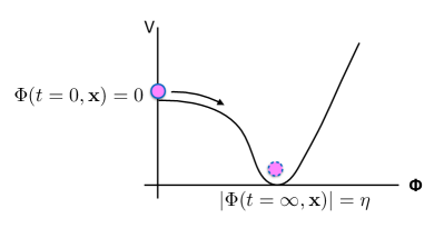
Figure 10: Simplified sketch of the Higgs potential as a function of $|\Phi|$. The Higgs field starts at $\Phi=0$ and will roll down to the true vacuum at $|\Phi|=\eta$ which is a three-sphere (angular components of $\Phi$ have been suppressed in the drawing). A bubble that triggers the rolling corresponds to a spherical region in space where $\Phi\neq 0$ but with no difference in energy as described in Ref. Zhang et al. (2019).

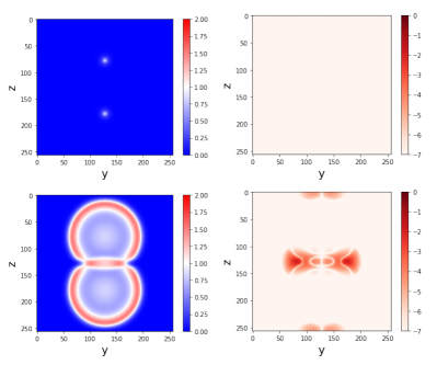
Figure 11: Cross-sectional plot of the magnitude of the Higgs field when two bubbles are nucleated (top left panel) with vanishing magnetic field energy density everywhere (top right panel). The bubbles grow and eventually collide (bottom left panel shows the Higgs field magnitude) and magnetic fields are produced in the collision region (bottom right panel). Periodic boundary conditions are imposed on the lattice, so the bubbles also collide on the top and the bottom of the plots.

The next step is to generate a stochastic distribution of bubbles, solve the classical equations of motion, evaluate the magnetic field and its properties. Fig. 12 shows that the average energy density in magnetic fields grows with time and reaches $\sim 6\%$ of the total energy density by the end of the simulation. (Longer duration runs were prohibitively expensive.) A point made in Ref.  Zhang et al. (2019) is that most of the magnetic field energy is produced during the time when the Higgs field is oscillating around the true vacuum.

Fig. 13 shows the power spectrum (which is $k^{2}|B_{k}|^{2}/V$ with the conventions of Diaz-Gil et al. (2008b)) at various times in the simulation. The peak at very low $k$ implies magnetic field production that is coherent on scales comparable to the lattice size and appears in other simulations as well (see Fig. 13 in Ref. Zhang et al. (2019)). According to the discussion in Diaz-Gil et al. (2008b), the peak is generated at high $k$ and then evolves to smaller $k$ in what might be termed an “inverse cascade”. It would be of great interest to confirm and understand this phenomenon on analytic grounds but it is satisfying that the spectrum has a $k^{3}$ behavior for small $k$ as also indicated by Eq. (50).

One question is if the energy in electromagnetic fields produced at the EWPT should be thought of as being in classical electric and magnetic fields or in photons. Though the quantum particle nature is fundamental, it is legitimate to think of the fields as classical because we are solving classical equations of motion with the classical expectation value of the Higgs field as a source for the gauge fields. We can also estimate the occupation number of the shortest wavelength mode (with $k=k_{*}$) using Eq. (50): $N_{k}=(T_{\rm EW}/k_{*})^{4}\gg 1$ since the (comoving) cut-off length scale on the order of kpc is vastly larger than the thermal scale on the order of cms.

Besides the usual limitations of numerical simulations – small lattices, short run times – a strong limitation is that the simulations do not include fermions, a plasma, and the expanding cosmological background with a horizon. These essential elements may affect the ultimate predictions for the properties of the magnetic fields produced at the EWPT.

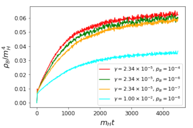
Figure 12: Average energy density in magnetic fields as a function of time for a few different choices of damping parameter ($\gamma$) and bubble nucleation probability ($p_{B}$). For details, see Zhang et al. (2019).

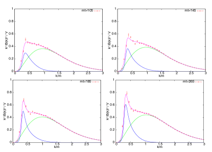
Figure 13: Four snapshots of the power spectrum (pink curve) from the simulations in Diaz-Gil et al. (2008b) show that the peak position ($\approx k_{*}$ in (50)) evolves to smaller $k$ with time. In this paper the authors also decompose the spectrum into a thermal component (green curve) and a non-thermal component (blue curve) that is coherent on long length scales. A functional fit that the authors provide gives $E_{M}(k)\propto k^{3}$ at small $k$, consistent with the estimate in Eq. (50). [Plot from Ref. Diaz-Gil et al. (2008b).]

III.1.5 Magnetic fields and matter genesis

Seemingly different physical phenomena sometimes have an underlying connection. This is the case for the generation of magnetic field helicity and the creation of cosmic baryon asymmetry Cornwall (1997); Vachaspati (2001); García-Bellido et al. (2004). Although baryon number is classically conserved in the standard model, a quantum anomaly can still violate it. The baryonic current density obeys,

$$\partial_{\mu}j^{\mu}_{B}=\frac{3}{32\pi^{2}}\left[g^{2}W^{a}_{\mu\nu}{\tilde{W}}^{a\mu\nu}-g^{\prime 2}Y_{\mu\nu}{\tilde{Y}}^{\mu\nu}\right]$$ (55)

where ${\tilde{W}}^{a\mu\nu}\equiv\epsilon^{\mu\nu\lambda\sigma}W_{\lambda\sigma}/2$. Now the term on the right-hand side can source baryon number changes. Eq. (55) can be integrated over all space to get the change in baryon number between some initial and final times,

$$\Delta N_{B}=3\Delta(CS)$$ (56)

where $CS$ stands for the Chern-Simons number,

$$CS = \frac{1}{32\pi^{2}}\int d^{3}x\,\epsilon_{ijk}\biggl{[}$$ (57)

$$\hskip-36.98866ptg^{2}\left(W^{aij}W^{ak}-\frac{g}{3}\epsilon^{abc}W^{ai}W^{bj}W^{ck}\right)-g^{\prime 2}Y^{ij}Y^{k}\biggr{]}$$

This formula can also be written in terms of the $W^{\pm}$, $Z$ and $A$ (electromagnetism) gauge fields Vachaspati and Field (1994). Then one gets different combinations of gauge fields on the right-hand side except for the ${\bf A}\cdot{\bf B}$ term, i.e. there is no baryon number anomaly due to the electromagnetic ${\bf E}\cdot{\bf B}$ (or $A{\tilde{A}}$) in (55). Then how can changes in baryon number be related to the helicity of electromagnetic magnetic fields?

The process of changing the Chern-Simons number can be visualized as the pair production of a monopole-antimonopole pair (that are connected by a Z-string in the electroweak model), then the pair is relatively twisted by $2\pi$, and allowed to annihilate again Vachaspati and Field (1994). In this process the Chern-Simons number changes by one. The very fact that monopoles appear in the intermediate step means that electromagnetic magnetic fields are present. The ultimate annihilation of the monopole-antimonopole releases the magnetic field that also carry the twist. In other words, the magnetic field is helical. Thus changes in Chern-Simons number are responsible for both baryon number production and the generation of helical magnetic fields Cornwall (1997); Vachaspati (2001); García-Bellido et al. (2004). The production of magnetic fields in Chern-Simons number changing processes has been studied in Copi et al. (2008); Chu et al. (2011) and during phase transitions in Diaz-Gil et al. (2008a, b); Mou et al. (2017); Kharzeev et al. (2019).

The change in the magnetic helicity density is related to the change in the baryon number density

$$\Delta h\sim-\frac{\Delta n_{B}}{\alpha}$$ (58)

where $\alpha\approx 1/137$ is the fine structure constant and $h$ is the magnetic helicity density defined in (21). The total helicity is generally conserved in MHD evolution and hence the helicity density will redshift with the Hubble expansion as $a^{-3}$ which is identical to the redshifting of the baryon number density. Since we know the present baryon density of the universe, and assuming zero baryon number and vanishing magnetic fields initially, (58) gives an estimate for the magnetic helicity density produced due to baryon number violation,

$$h_{\rm b}\sim-10^{-5}\,{\rm cm}^{-3}$$ (59)

The discussion above assumes that we start in the broken phase of the electroweak symmetry and then a process changes the Chern-Simons number. During the electroweak phase transition, however, we start in a phase where the electroweak symmetry is unbroken and electromagnetism isn’t even defined. Then we might expect differences in the numerical estimate of the magnetic helicity depending on the details of the phase transition.

To test the formation of helical magnetic fields at the EWPT, the authors of Ref. Mou et al. (2017) extended the standard model by including a CP violating interaction term $|\Phi|^{2}W{\tilde{W}}$ (group and Lorentz indices suppressed) in the electroweak Lagrangian and did not confirm (58). However, the reason is simple to understand and might indicate an interesting direction to explore (see Sec. V). Once the electroweak symmetry is broken, the $W^{a}$ gauge fields can be re-expressed in terms of the $W^{\pm}$, $Z$ and electromagnetic $A$ gauge fields. Then the extra interaction term explicitly provides an interaction $|\Phi|^{2}A{\tilde{A}}$ and the dynamics of $\Phi$ can directly source helicity in the magnetic field. The result of the simulation is a sum of the helicity due to changes in the Chern-Simons number and the helicity due to this direct sourcing and it is not surprising that the relation between changes of Chern-Simons number and magnetic helicity in (58) is not verified. A way around this issue would be to change the additional interaction term to $|\Phi|^{2}(g^{2}W{\tilde{W}}-g^{\prime 2}Y{\tilde{Y}})$ as this will eliminate the direct $|\Phi|^{2}A{\tilde{A}}$ coupling. Such a simulation remains to be done at this point in time. We will return to this topic in Sec. V.

Finally let us compare the estimate in (58) with the helicity in inter-galactic magnetic fields that may be implied by observations. For our numerical estimates we will use the most conservative field strength of $B_{\lambda}\sim 10^{-19}\,{\rm G}$ with $\lambda\sim 1\,{\rm Mpc}$ Finke et al. (2015). Since MHD evolution implies that magnetic fields evolve to maximal helicity, we have with (22), (13), and $k_{1}=2\pi/\lambda$ where $\lambda=3\times 10^{24}\,{\rm cm}$,

$$k_{1}H_{M}(k_{1})=2E_{M}(k_{1})=\frac{1}{k_{1}}B_{\lambda}^{2}\approx 10\,{\rm cm}^{-3}$$ (60)

The helicity density is defined by (21) and to integrate over all $k$, we need to assume a spectrum for $H_{M}$. Let us take $E_{M}\propto k^{n+1}$ and $H_{M}\propto k^{n}$ with electroweak physics suggesting $n=2$ as in (50). Then, the observed helicity is at least,

$$h_{\rm obs}\approx\frac{k_{1}H_{M}(k_{1})}{n+1}\left(\frac{k_{*}}{k_{1}}\right)^{n+1}\sim 10^{3n+3}\,{\rm cm}^{-3}\gg h_{\rm b}$$ (61)

where $k_{*}\approx 2\pi/(1\,{\rm kpc})$ corresponds to the short distance cutoff due to dissipation and $h_{\rm b}$ is the helicity resulting from baryogenesis in (59). These estimates show that the magnetic helicity produced in association with baryogenesis is too small to account for the magnetic helicity that must accompany observed magnetic fields. This statement comes with the important implication that the standard model of particle physics may need to be extended to include stronger CP violation if it is to successfully explain observed inter-galactic magnetic fields, perhaps along the lines of Sec. V.

III.2 Magnetic field generation at QCD and inflationary epochs

A number of ideas have been proposed for magnetic field generation during the QCD epoch Quashnock et al. (1989); Cheng and Olinto (1994); Sigl et al. (1997); Tevzadze et al. (2012); Forbes and Zhitnitsky (2000); Miniati et al. (2018). Early ideas Quashnock et al. (1989); Cheng and Olinto (1994); Sigl et al. (1997) were based on the assumption of a first order QCD phase transition in which bubbles of the hadronic phase grow within the ambient quark phase. In this process there is charge separation because the quarks carry a small net positive charge and interact with the bubble walls while the leptons carry a small net negative charge and are oblivious to the bubbles. It is argued that the dynamics of the bubble walls will generate turbulence in the charge-separated medium, resulting in electric currents and then magnetic fields. An estimate Cheng and Olinto (1994) gives $10^{-20}\,{\rm G}$ on a coherence scale $\sim 1\,{\rm kpc}$. Scenarios based on a first order QCD phase transition, however, need to be re-examined as the understanding at present is that the transition from the quark phase to the hadron phase is a crossover and not a phase transition (e.g. see Rischke (2004); Fukushima and Hatsuda (2010)). Other ideas to generate magnetic fields invoke ferromagnetic domain walls in non-perturbative QCD Forbes and Zhitnitsky (2000); Tevzadze et al. (2012), and more recently, axion interactions during the hadronization of quarks at the QCD epoch Miniati et al. (2018).

A number of authors have studied the generation of magnetic fields during inflation by coupling the inflaton dynamics to that of the electromagnetic field (see Turner and Widrow (1988); Ratra (1992); Adshead et al. (2016) and the reviews Widrow (2002); Durrer and Neronov (2013); Subramanian (2016)). An advantage is that strong fields can be produced on large coherence scales if certain field couplings and interaction strengths are postulated in addition to the usual assumptions underlying inflation. The disadvantage is that there are few guiding principles that can tell us whether the new interactions and coupling strengths are indeed realized. However, if strong, coherent fields are observed, magnetic fields generated during inflation or its alternatives may be the only recourse.

IV MHD evolution of cosmic magnetic fields

The cosmological evolution of magnetic fields is commonly discussed in the MHD approximation where the displacement current $\partial_{t}{\bf E}$ is neglected in Maxwell’s equations Brandenburg et al. (1996) (also see Appendix B of Banerjee and Jedamzik (2004)). We will restrict our attention to a spatially flat expanding universe for which the line element can be written as,

$$ds^{2}=a^{2}(\eta)\,(d\eta^{2}-d{\bf x}^{2})$$ (62)

where $a(\eta)$ is the scale factor and $\eta$ is the conformal time (not to be confused with the VEV of the Higgs field in earlier sections). We also define “comoving” quantities (denoted by a $c$ subscript),

$${\bf B}_{c}=a^{2}{\bf B},\ {\bf E}_{c}=a^{2}{\bf E},\ {\bf v}_{c}={\bf v},\ \rho_{c}=a^{4}\rho,\ p_{c}=a^{4}p$$ (63)

where $\rho$ and $p=\rho/3$ are the energy density and pressure for a radiation fluid. Then the equation for the magnetic field is

$$\partial_{\eta}{\bf B}_{c}=\nabla\times({\bf v}_{c}\times{\bf B}_{c})+\frac{1}{\sigma_{c}}\nabla^{2}{\bf B}_{c}$$ (64)

where $\eta$ denotes the conformal time, related to the cosmic time $t$ by $dt=a(t)d\eta$, $\sigma_{c}=a\sigma$ is the comoving electrical conductivity of the cosmological plasma at temperature $T$. The first term on the right-hand side of (64) is called the “advection” term. As a plasma element moves, it carries the magnetic field with it while conserving flux Jackson (1975). The second term on the right-hand side is the “diffusion” term since if we ignore the advection term, the MHD equation reduces to a diffusion equation. The diffusion time scale is set by the electrical conductivity of the plasma. For large enough electrical conductivity, only the advection term comes into play and then we say that the magnetic field is “frozen in” the plasma. The evolution can be highly non-trivial even in the frozen in limit because the fluid velocity field might be turbulent and the magnetic field would get highly tangled, even as the magnetic field backreacts on the flow.

The plasma Navier-Stokes equation for a radiation-baryon fluid of comoving energy density $\rho_{c}$ and comoving pressure $p_{c}$ in the MHD approximation is Brandenburg et al. (1996),

$$\partial_{\eta}{\bf S}=-(\nabla\cdot{\bf v}_{c}){\bf S}-({\bf v}_{c}\cdot\nabla){\bf S}-\nabla p_{c}+(\nabla\times{\bf B}_{c})\times{\bf B}_{c}$$ (65)

where ${\bf S}\equiv(\rho_{c}+p_{c})\gamma^{2}{\bf v}_{c}$ and $\gamma=1/\sqrt{1-{\bf v}_{c}^{2}}$ is the Lorentz boost factor. The last term on the right-hand side describes the Lorentz force on a plasma element due to the magnetic field because $\nabla\times{\bf B}_{c}={\bf J}_{c}$. We have ignored the viscosity term and other non-ideal terms but these can be included.

The continuity equation takes the form,

$$\partial_{\eta}S^{0}+\nabla\cdot(S^{0}{\bf v}_{c})+\frac{a^{\prime}}{a}\left(4p_{c}-\frac{S^{0}}{\gamma^{2}}\right)-\partial_{\eta}p_{c}$$ (66)

$$\hskip-85.35826pt=-(\nabla\times{\bf B}_{c})\cdot{\bf E}_{c}$$

where $S^{0}\equiv(\rho_{c}+p_{c})\gamma^{2}$ and $a^{\prime}=da/d\eta$. With $p_{c}=\rho_{c}/3$ for a radiation fluid, and assuming non-relativistic flows ($\gamma\approx 1$), this equation simplifies to

$$\partial_{\eta}\rho_{c}+\frac{4}{3}\nabla\cdot(\rho_{c}{\bf v}_{c})=-(\nabla\times{\bf B}_{c})\cdot{\bf E}_{c}$$ (67)

By combining Ohm’s law in the rest frame of the fluid with Ampere’s law (in the MHD approximation) , we can write

$${\bf E}_{c}=\frac{1}{\sigma_{c}}{\bf J}_{c}-{\bf v}_{c}\times{\bf B}_{c}=\frac{1}{\sigma_{c}}(\nabla\times{\bf B}_{c})-{\bf v}_{c}\times{\bf B}_{c}.$$ (68)

The electrical conductivity of the cosmological plasma has been estimated in Turner and Widrow (1988); Ahonen and Enqvist (1996); Baym and Heiselberg (1997); Arnold et al. (2000). The result is

$$\sigma\sim\frac{T}{\alpha\ln(1/\alpha)},$$ (69)

where the logarithmic correction can be found in Baym and Heiselberg (1997); Arnold et al. (2000). This calculation assumes that Rutherford scattering dominates and determines the mean free path. Cosmological events such as $e^{+}e^{-}$ annihilation at $T\approx 0.1\,{\rm MeV}$, lead to a sudden drop in the electron number density and then Thomson, not Rutherford, scattering determines the mean scattering time. Since $n_{e}/n_{\gamma}\approx 10^{-10}$ after annihilation, the electrical conductivity becomes Turner and Widrow (1988)

$$\sigma\sim 10^{-10}\frac{m_{e}}{e^{2}},\ \ T\lesssim 0.1\,{\rm MeV}$$ (70)

However, Rutherford scattering cross section is proportional to $1/v^{4}\sim(m_{e}/T)^{2}$ while Thomson scattering is independent of $v$. As the universe cools, at $T\sim 1\,{\rm eV}$, Rutherford scattering dominates again, but now it is close to the epoch of recombination when the free electron density will once again drop dramatically by a factor $\sim 10^{-5}$ to that of residual ionization.

In spite of the dramatic drops in electrical conductivity, the magnetic field diffusion time scale is much larger than the Hubble time on the length scales of interest to us ($\gtrsim 1\,{\rm kpc}$ today). The diffusion length scale, $l_{\rm diff}$, can be obtained by comparing the left-hand side of (64) to the diffusion term on the right-hand side,

$$l_{\rm diff}(t)\sim\sqrt{\frac{t}{\sigma}}=t\,\sqrt{\frac{\alpha|\ln(\alpha)|}{tT}}$$ (71)

(Note that $l_{\rm diff}$ is the physical, not comoving, length scale.) For example, $l_{\rm diff}(t_{0})\sim 10^{12}\,{\rm cm}$ where $t_{0}$ denotes the present epoch and $l_{\rm diff}(t_{\rm EW})\sim 10^{-6}\,{\rm cm}$ which is much smaller than the electroweak horizon of $\sim 1\,{\rm cm}$. Diffusion is unimportant on length scales larger than $l_{\rm diff}$, while it must be taken into account in the MHD evolution on length scales smaller than $l_{\rm diff}$.

Diffusion isn’t the only dissipative mechanism for the magnetic field. Magnetized plasmas have several excitation modes, called “magnetosonic” modes, that can propagate and dissipate on various time-scales. A tangled magnetic field will excite these modes during evolution and then the modes will dissipate, with the dissipation time-scale depending on the type of mode. Without going into details, the dissipation length scale for these modes is in the ${\rm pc}$ to ${\rm kpc}$ range. Thus the power spectrum of cosmological magnetic fields at the present epoch is expected to be cut off for $k\gtrsim 1-10^{3}\,{\rm kpc}^{-1}$ Jedamzik et al. (1998).

An important result of MHD is that magnetic helicity is conserved during evolution. This may be proved quite simply in the $\sigma\to\infty$ limit

$$\partial_{t}\int d^{3}x\,{\bf A}\cdot{\bf B} = -2\int d^{3}x\,{\bf E}\cdot{\bf B}$$

$$= -\frac{2}{\sigma}\int d^{3}x\,{\bf J}\cdot{\bf B}\to 0,\ {\rm as}\ \sigma\to\infty$$

using Ohm’s law as in (68). However, the more remarkable feature of magnetic helicity is that it is conserved in a variety of applications even for finite conductivity. Indeed, MHD experts view magnetic helicity conservation as more robust than energy conservation Choudhuri (1998).

The evolution of cosmological magnetic fields has been studied using a combination of analytical and numerical techniques Dimopoulos and Davis (1997); Subramanian and Barrow (1998); Brandenburg et al. (1997); Son (1999); Christensson et al. (2001, 2005); Banerjee and Jedamzik (2003); Campanelli (2004); Banerjee and Jedamzik (2004); Campanelli (2007); Jedamzik and Sigl (2011); Kahniashvili et al. (2010, 2012); Tevzadze et al. (2012); Kahniashvili et al. (2013); Saveliev et al. (2012); Campanelli (2014); Saveliev et al. (2013); Brandenburg et al. (2015); Campanelli (2016); Brandenburg and Kahniashvili (2017); Kahniashvili et al. (2017); Brandenburg et al. (2017a); Brandenburg et al. (2019); Brandenburg et al. (2017b); Reppin and Banerjee (2017); Achikanath Chirakkara et al. (2021). Here we sketch some of the main results, ignoring the finer points and focusing on magnetic field spectra that fall off on large length scales, $E_{M}\propto k^{n}$ with $n>0$, and peak on some small length scale.

IV.1 Sketch of magnetic field evolution

Initial conditions: Stochastic, statistically isotropic magnetic fields are described by two spectra, $E_{M}(k,t)$ and $H_{M}(k,t)$. Any mechanism for generating magnetic fields should provide these functions at the initial time. Additionally, the velocity field is also described by two spectra: the power spectrum and the kinetic helicity spectrum. Even though the set of initial conditions that have been studied is not exhaustive, the results give a fairly good idea of what to expect from MHD evolution. Ref. Banerjee and Jedamzik (2004) also discusses magnetic field evolution through cosmological events such as $e^{+}e^{-}$ annihilation, recombination, dissipation, etc. while Ref. Brandenburg et al. (2019) considers non-vanishing kinetic helicity as an initial condition.

Non-helical evolution: First consider the case of non-helical magnetic fields, $H_{M}(k)=0$, and vanishing velocity field at the initial time. The magnetic field will induce fluid flow and turbulence, and the full non-linear system of equations (64), (65) and (66) has to be solved. This setup is called “magnetically dominated decaying MHD turbulence” or “freely decaying MHD turbulence”. The detailed evolution of the magnetic power spectrum depends on the initial conditions. However, the general features of the evolution can be sketched as in Fig. 14. The peak of the spectrum at the inertial scale, $k_{\rm in}$, moves to smaller $k$ for two reasons: first, the power on small length scales dissipates more efficiently, and second, there is a weak inverse cascade that actually shifts the peak to smaller $k$ Olesen (1997); Brandenburg et al. (2015). These factors lead to

$$k_{\rm in}(\eta)\propto\eta^{-1/2},\ \ {\rm nonhelical\ case}.$$ (72)

The $k$-dependence of the spectrum for $k<k_{\rm in}(\eta)$ depends on the initial conditions. With $E_{M}\propto k^{p}$ at the initial time for small $k$ where $p\geq 4$, the spectrum evolves to the Batchelor spectrum, $E_{M}\propto k^{4}$ (see Saveliev et al. (2012) and the Supplemental Material to Brandenburg et al. (2015)). For $p=2$, called “non-helical white noise spectrum”, the simulations in Brandenburg et al. (2017b) do not find an inverse cascade and the spectrum stays $E_{M}\propto k^{2}$ even upon evolution. This suggests that for the non-helical case and with $p<4$, the power spectrum will remain $E_{M}\propto k^{p}$ even with evolution.

The non-helical inverse cascade has been examined critically in Reppin and Banerjee (2017). It is found that the inverse cascade depends on the Prandtl number, defined as the ratio of the viscosity and magnetic diffusivity, and decreases in efficiency as the Prandtl number increases. Ref. Reppin and Banerjee (2017) suggests that the non-helical inverse cascade may be completely suppressed at the Prandtl numbers relevant to cosmology ($\sim 10^{8}(T/{\rm keV})^{-3/2}$).

If initially the velocity field does not vanish, and is perhaps helical, the evolution can be more involved. For example, in case of initial kinetic helicity, the magnetic field can develop helicity that is opposite to the kinetic helicity on large length scales. The conservation of total helicity then implies compensating magnetic helicity on short length scales Brandenburg et al. (2019).

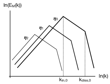
Figure 14: The evolution of the comoving power spectrum of non-helical magnetic fields shown at three (conformal) times $\eta_{0}<\eta_{1}<\eta_{2}$. The peak of the spectrum dissipates and also moves to smaller (comoving) $k$ in proportion to $\eta^{-1/2}$. As a result the power on large length scales increases in what is termed a “non-helical inverse cascade”. The spectrum evolves to $E_{M}\propto k^{4}$ at small $k$ for a broad range of initial conditions in which $E_{M}\propto k^{p}$ with $p\geq 4$ at the initial time.

Helical evolution: A general feature is that magnetic fields evolve towards “maximal helicity” (see (22)), while total helicity stays conserved. This means that $H_{M}(k)$ evolves non-trivially with time while its integral over all $k$ stays constant. To approach maximal helicity $E_{M}(k)$ evolves so that

$$E_{M}(k,\eta)\to\frac{k}{2}|H_{M}(k,\eta)|$$ (73)

Once the field achieves maximal helicity, it stays maximally helical, while power (and helicity) is transferred to larger length scales in an inverse cascade as depicted in Fig. 15 where the whole spectrum simply shifts to the left. This feature can be seen using the conservation of magnetic helicity. We take the form of the time-dependent power spectrum to be

$$E_{M}(k,\eta)={\cal E}(\eta)\left(\frac{k}{k_{\rm in}(\eta)}\right)^{n},\ \ 0\leq k\leq k_{\rm in}(\eta)$$ (74)

where $n>0$ is left unspecified. (The power for $k>k_{\rm in}$ can be included but we ignore it here.) Assuming that the helicity is the same sign for all $k$, maximal helicity implies

$$H_{M}(k,\eta)=\frac{2}{k}E_{M}(k,\eta)=\frac{2}{k}{\cal E}(\eta)\left(\frac{k}{k_{\rm in}(\eta)}\right)^{n}.$$ (75)

The total helicity is conserved,

$${\rm constant}=\int_{0}^{k_{\rm in}}dk\,H_{M}(k,\eta)=\frac{2}{n}{\cal E}(\eta)$$ (76)

Therefore ${\cal E}$ is a constant and the peak of the power spectrum at $k=k_{\rm in}(\eta)$ does not dissipate. The energy density defined in (19) decays with time as $k_{\rm in}(\eta)$ which has been determined by simulations Christensson et al. (2001); Kahniashvili et al. (2013),

$$k_{\rm in}(\eta)\sim k_{\rm in}(\eta_{0})\left(\frac{\eta_{0}}{\eta}\right)^{2/3},\ \ {\rm helical\ case}$$ (77)

where $\eta_{0}$ is the initial conformal time. The $2/3$ exponent in the helical case should be contrasted with the $1/2$ exponent in the non-helical case given in (72).

As in the non-helical case, the evolution leads to $E_{M}\propto k^{4}$ if initially $E_{M}\propto k^{p}$ with $p\geq 4$. In simulations with magnetic fields that are initially helical with white noise spectrum ($p=2$), the spectrum evolved to $E_{M}\propto k^{4}$ once the field became maximally helical, suggesting that the Batchelor spectrum is an attractor (see Run G in Brandenburg et al. (2017b)).

Figure 15: The evolution of the comoving power spectrum of helical magnetic fields at three different times $\eta_{0}<\eta_{1}<\eta_{2}$. The peak of the spectrum moves to smaller comoving $k$ but does not dissipate once the field becomes maximally helical. As a result the power on large length scales increases in what is termed an “inverse cascade”. The spectrum evolves to $E_{M}\propto k^{4}$ at small $k$ for a broad range of initial conditions in which $E_{M}\propto k^{p}$ with $p\geq 4$ at the initial time.

IV.2 Dissipation and the integral scale

The dissipation of perturbations overlaid on a smooth cosmological magnetic field, taking into account the cosmological plasma and the neutrino and photon fluids, has been studied in Ref. Jedamzik et al. (1998). The perturbations can be decomposed into plasma Alfvén and magnetosonic (fast and slow) modes. These modes will propagate and interact with neutrinos prior to neutrino decoupling, and with photons prior to recombination, and will damp out the perturbations on small wavelengths. The damping length scale depends on the particular excitation mode, the epoch of interest, and the strength of the background magnetic field.

The framework of a perturbation on a smooth background magnetic field as adopted in Jedamzik et al. (1998) is not directly relevant to the case of magnetic fields generated at phase transitions. Instead we are interested in power spectra that are peaked on small length scales, e.g. $E_{M}\propto k^{3}$. In this case, Banerjee and Jedamzik Banerjee and Jedamzik (2004) estimate the “integral” scale of the spectrum – the length scale on which the spectrum is peaked – in the turbulent regime and also in the viscous regime in which fluid flow experiences a drag due to free streaming particles such as neutrinos and photons. The comprehensive analysis of Banerjee and Jedamzik (2004) also places MHD evolution in a cosmological setting, taking account various cosmological episodes such as neutrino decoupling, $e^{+}e^{-}$ annihilation, Hydrogen recombination, and the transition from radiation to matter domination.

The picture developed in Ref. Banerjee and Jedamzik (2004) is that there is a direct (Kolmogorov) cascade of energy for length scales smaller than the integral scale, $L$, and as modes with length scale just below $L$ lose their energy, the peak of the spectrum shifts to longer length scales, i.e.  the integral scale $L$ grows. Based on a combination of analytical and numerical techniques, they argue that the integral scale can be estimated by equating the turnover timescale for eddies on the integral scale to the Hubble time,

$$v(L)/L\approx H$$ (78)

where $v(L)$ is the fluid velocity on the integral scale $L$. In the turbulent regime, $v(L)\approx v_{A}$, the Alfv́en velocity defined by $v_{A}=B/\sqrt{4\pi(\rho+p)}$ where $\rho$ and $p$ are the energy density and pressure of the fluid. In the viscous regime, $v(L)\approx R_{e}v_{A}$ where $R_{e}$ is the Reynolds number evaluated with the Alfv́en velocity. An important outcome of this analysis is that the magnetic field strength at the present epoch is related to the integral scale today,

$$B_{0}\approx 5\times 10^{-12}\,{\rm G}\,\left(\frac{L_{0}}{1\,{\rm kpc}}\right).$$ (79)

Their final estimate for the integral scale for magnetic fields generated at the EWPT depends on the initial magnetic power spectrum and the magnetic helicity, and lies in the $0.1\,{\rm pc}$ to $10\,{\rm kpc}$ range (see Figs. 12-15 in Banerjee and Jedamzik (2004)). For maximally helical fields with $1\%$ of the total energy density and with $E_{M}\propto k^{2}$ at the EWPT, they estimate the comoving integral length scale to be $\sim 10\,{\rm kpc}$, whereas for non-helical fields it is $\sim 1\,{\rm pc}$. The magnetic field strength at the integral scale can then be evaluated using (79).

The evolution of cosmological magnetic fields eventually becomes entangled with the formation of cosmological structures. This process, together with observational implications, has been studied using numerical simulations in Ref. Vazza et al. (2017).

IV.3 Speculations on evolution of $E_{M}\propto k^{3}$ spectrum

As described in Sec. III, magnetic fields generated at the EWPT are expected to have $E_{M}\propto k^{3}$ for small $k$ and energy density of a few percent of the total energy density. In addition, the magnetic field may be helical though the fractional helicity is small if it only arises due to baryon number violating processes (see Sec. V). The evolution of the integral scale and strength of magnetic fields with these initial conditions has been studied in Ref. Banerjee and Jedamzik (2004) with an estimate of $\sim 10\,{\rm pc}$ for the integral scale (same as coherence scale), and $\sim 10^{-13}\,{\rm G}$ magnetic field strength at the integral scale. These estimates depend on the initial magnetic helicity. For initial maximal helicity, the integral scale is $\sim 10\,{\rm kpc}$ and field strength $\sim 10^{-10}\,{\rm G}$.

The evolution of the power spectrum, $E_{M}(k,\eta)$, has not been discussed in Ref. Banerjee and Jedamzik (2004). However, based on the results of Brandenburg et al. (2017b) we might anticipate some features of the power spectrum. As an initial condition we assume that $E_{M}(k,\eta_{0})\propto k^{3}$ up to $k=k_{\rm in}$. For $k>k_{\rm in}$, the spectrum falls off according to the Kolmogorov spectrum $\propto k^{-5/3}$, and then a sharper fall off ensues at the dissipation scale $k_{\rm diss}$ such that modes with $k>k_{\rm diss}$ can release their energy into heat. At very low $k$, with evolution I expect that the initial spectrum $\propto k^{3}$ will be maintained because these are long length scales and the time scales will be correspondingly longer. In the very low $k$ region, the evolution should be as for “acausal” spectra in Refs. Brandenburg et al. (2018b); Brandenburg et al. (2020). The integral scale, however, shifts to smaller $k$ as happens in an inverse cascade. For $k$ somewhat below $k_{\rm in}(\eta)$, we expect the magnetic field to develop towards maximal helicity and a $k^{4}$ spectrum Brandenburg et al. (2017b). For $k>k_{\rm in}(\eta)$, the Kolmogorov spectrum and the dissipative spectrum hold. These features are sketched in Fig. 16. These speculations imply a new scale that we denote by $k_{*}(\eta)$ where the $k^{3}$ spectrum changes to a $k^{4}$ spectrum. With time we expect $k_{*}$ to move to smaller $k$ to maintain the $k^{4}$ power law for $k_{*}<k<k_{\rm in}$. If the magnetic field is near maximally helical at the initial time, it may also happen that the peak at $k_{\rm in}(\eta)$ actually grows in amplitude as the integral scale shifts to lower $k$. It would be of great interest to examine this case in more detail by numerical simulations.

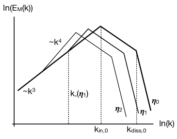
Figure 16: A guess for the evolution of the comoving $E_{M}\propto k^{3}$ spectrum with partial helicity generated at the EWPT at three different times $\eta_{0}<\eta_{1}<\eta_{2}$. The peak of the spectrum decays if there is only partial helicity and moves to the left due to an inverse cascade. The helicity in the peak region becomes maximal and the power spectrum in this region develops to $k^{4}$, while the spectrum at the smallest $k$ retains its initial $k^{3}$ form. The time-dependent $k_{*}$ denotes the location where the transition from $k^{3}$ to $k^{4}$ occurs.

IV.4 Qualitative constraint plot

Ideally a constraint plot maps out the regions in the $\lambda$-$B_{\lambda}$ plane (equivalently the $k$-$E_{M}(k)$ plane because of (13)) that are disallowed or else suggested by observations. However, as discussed in Sec. II, to translate an observational constraint to a region of the $\lambda-B_{\lambda}$ plane, we need to know the window function and this is not always available and may not be simple. Instead a constraint may be derived by comparing observations to the results of simulations that are done by assuming a certain form of $E_{M}(k)$, e.g. the magnetic field has fixed field strength and is uniform in domains of size 1 Mpc. Hence a constraint plot should be treated with a certain amount of caution. Nonetheless a constraint plot can be very helpful to quickly visualize the overall status of cosmological magnetic fields. With this disclaimer, we sketch current constraints and other markers in the $\lambda-B_{\lambda}$ plane in Fig. 17.

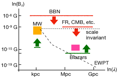
Figure 17: Cosmological magnetic fields with $\lambda\sim{\rm kpc}$ and $B_{\lambda}\sim 10^{-10}\,{\rm G}$ may directly explain, i.e. with minimal dynamo amplification, the galactic magnetic field, and may help resolve the present Hubble tension due to baryon clustering at Hydrogen recombination. This region is denoted by the golden rectangle marked by “MW” (for Milky Way). Big bang nucleosynthesis (BBN) constrains $B_{\lambda}\lesssim 10^{-6}\,{\rm G}$ on all scales, while other observations roughly constrain $B_{\lambda}\lesssim 10^{-9}\,{\rm G}$ on Mpc to Gpc scales. Blazar spectral measurements place a lower bound $\sim 10^{-16}\,{\rm G}$ for $\lambda$ in the Mpc to Gpc range, or instead a lower bound of $\sim 10^{-15}\,{\rm G}$ on kpc scales, and assumes that plasma instabilities do not play a role. Magnetic helicity measurements are uncertain but, if confirmed, would lie in the region of the pink rectangle. If the cosmological magnetic field is scale invariant, as in some inflationary models, and also passes through the golden rectangle, it would correspond to the horizontal dotted line and is pressured by several constraints. If the cosmological magnetic field has a blue $k^{3}$ or $k^{4}$ spectrum as might be expected from the EWPT, it may correspond to a shape like the dashed curve. This constraint plot is meant to be schematic as there is considerable uncertainty in the numbers and also the caveats mentioned in the text. For example, $B_{\lambda}$ may be below the blazar bound shown by the green line at $\lambda\sim{\rm Mpc}$ since small scale (kpc) magnetic fields can instead explain the absence of blazar halos.

V Amplifying magnetic helicity

We have seen in Sec. III that magnetic fields can be generated during the EWPT with relatively large energy density and with $k^{3}$ power spectrum. Without magnetic helicity though, the evolution discussed in Sec. IV.1 shows that the field strength on large ($\sim{\rm Mpc}$) length scales will be very weak. Magnetic helicity can significantly change these estimates as it modifies the evolution by producing an inverse cascade that pushes the coherence scale to larger length scales and also increases the power on these scales. The connection of magnetic field generation with baryogenesis described in Sec. III shows that the standard model has all the ingredients necessary for generating magnetic helicity. However the numbers don’t quite work out as discussed in Sec. III.1.5 and the magnetic helicity produced during baryogenesis falls short of what is needed by many orders of magnitude. This failure, as well as the failure of the standard model to explain the cosmic baryon asymmetry, the dark matter problem and neutrino masses, suggests that the standard model needs to be extended.

One possibility relevant to magnetic fields is that the electroweak plasma contains chiral fermions with net chirality  Vachaspati and Vilenkin (2021). Then the chiral-vortical Vilenkin (1979) and chiral-magnetic Vilenkin (1980) effects may come into play, effectively providing an electric current that is proportional to the magnetic field and this can amplify the magnetic helicity Joyce and Shaposhnikov (1997); Tashiro et al. (2012); Dvornikov and Semikoz (2014, 2017); Rogachevskii et al. (2017); Brandenburg et al. (2017a); Schober et al. (2018). However, as noted in Ref. Brandenburg et al. (2017a) the helicity amplification is limited by the assumed initial chirality of the medium and is further limited due to chirality flipping Boyarsky et al. (2020a, b). Alternately, as we have mentioned in Sec. IV.1, kinetic helicity can separate magnetic helicity of opposite signs. Perhaps in chiral scenarios this can result in amplified magnetic helicity on large length scales that is approximately compensated by opposite magnetic helicity on small scales such that the net magnetic helicity is not too large.

Yet another possibility is that there are new CP violating interactions in particle physics. A simple way to introduce additional CP violation in the standard model is to add the interactions,

$$L_{\rm CP} = \frac{|\Phi|^{2}}{\eta^{2}}\biggl{[}\beta_{\rm CS}\left(c_{w}^{2}W_{\mu\nu}^{a}{\tilde{W}}^{a\mu\nu}-s_{w}^{2}Y_{\mu\nu}{\tilde{Y}}^{\mu\nu}\right)$$ (80)

$$\hskip 14.22636pt+\beta_{A}\left(s_{w}^{2}W_{\mu\nu}^{a}{\tilde{W}}^{a\mu\nu}-c_{w}^{2}Y_{\mu\nu}{\tilde{Y}}^{\mu\nu}\right)\biggr{]}$$

where $\beta_{\rm CS}$ and $\beta_{A}$ are coupling strengths, $s_{w}^{2}\equiv\sin^{2}\theta_{w}\approx 0.23$, $c_{w}\equiv\cos\theta_{w}$, and $\eta$ is the VEV of $\Phi$. A reason for the particular grouping of terms in (80) is that the Chern-Simons (CS) combination is natural for baryogenesis, while the other combination is natural for magnetic helicity generation. To see this, let us work in the unitary gauge where $\Phi\propto(0,1)^{T}$, suppress Lorentz indices, and assume $W^{1}=0=W^{2}$. Then we can rewrite the groupings in terms of $Z_{\mu\nu}$ and $A_{\mu\nu}$ (written as $Z$ and $A$),

$$c_{w}^{2}W^{a}{\tilde{W}}^{a}-s_{w}^{2}Y{\tilde{Y}} = c_{2w}Z{\tilde{Z}}+s_{2w}A{\tilde{Z}}$$

$$s_{w}^{2}W^{a}{\tilde{W}}^{a}-c_{w}^{2}Y{\tilde{Y}} = -c_{2w}A{\tilde{A}}+s_{2w}A{\tilde{Z}}$$

where $c_{2w}=\cos(2\theta_{w})$ and $s_{2w}=\sin(2\theta_{w})$. The Chern-Simons combination of terms directly couples the Higgs to $Z{\tilde{Z}}$ but not to $A{\tilde{A}}$, while the other combination provides a direct coupling to the electromagnetic $A{\tilde{A}}$ but not to $Z{\tilde{Z}}$. As the phase transition proceeds and the Higgs rolls down on its potential, the first group of interactions in $L_{\rm CP}$ will generate changes in the Chern-Simons number that will lead to baryogenesis via (56) and (anomalous) helical magnetic field production as discussed in (58). The second combination of interactions in $L_{\rm CP}$ will directly generate helical magnetic fields. In fact the simulations of Ref. Mou et al. (2017) were done with $\beta_{A}/\beta_{\rm CS}=-\tan^{2}\theta_{w}$ and hence included only the $W{\tilde{W}}$ terms in $L_{\rm CP}$. The simulations resulted in magnetic helicity production that was uncorrelated with the baryon number production. This is not surprising since with this choice of coefficients there is direct magnetic helicity production due to the $\beta_{A}$ term in (80) and also weaker helicity production due to the indirect coupling through changes in the Chern-Simons number. It is of immense interest to investigate these simulations more thoroughly to determine if there is a sweet spot that can accommodate both the baryon number of the universe and the helical magnetic fields indicated by blazar observations. If there is such a sweet spot, the observation of cosmological magnetic fields might lead to the discovery of CP odd operators in fundamental particle interactions, another beautiful inner space/outer space connection!

The additional couplings in $L_{\rm CP}$ are constrained by collider data as they provide new channels for the Higgs boson to decay into two photons, and to a $Z$ boson and a photon. At the moment the experimental constraints are roughly $\beta_{\rm CS},\beta_{A}\lesssim 10^{-2}$ as in Ref. Gan et al. (2017). Constraints on $\beta_{\rm CS}$ and $\beta_{A}$ from the observation of magnetic fields and baryon asymmetry would provide helpful guidance to particle experiments that should ultimately measure these parameters Bishara et al. (2014).

It is difficult to predict the magnetic helicity spectrum that will be induced by the terms in (80) without detailed analyses. However it is still useful to make a guess that can serve as a strawman for when such analyses are carried out. We have already discussed that the dynamics of the electroweak symmetry breaking leads to significant magnetic fields. Such fields are not helical. With the $L_{\rm CP}$ extension, additional magnetic fields are generated due to the $\beta_{A}$ coupling. Such magnetic fields are helical. The $\beta_{\rm CS}$ coupling also gives rise to helical magnetic fields but this contribution is small. So the overall picture is that the $\beta_{A}$ coupling leads to helical magnetic fields that are diluted by the non-helical fields produced by the Higgs dynamics in the un-extended standard model. A simple guess is that the magnetic helicity spectrum is proportional to the power spectrum with the constant of proportionality determined by the coupling constant $\beta_{A}$,

$$H_{M}(k) = \beta\frac{2}{k}E_{M}(k)$$ (81)

$$= \frac{2\beta\rho_{EW,B}}{k_{*}^{2}}\left(\frac{k}{k_{*}}\right)^{2},\ \ k\leq k_{*}$$

where we have used (50) in the second line, and $\beta\sim\pm 10^{-2}$ represents the coupling constants and the sign will depend on the sign of $\beta_{A}$. It would be of interest to study the evolution of cosmological magnetic fields with the initial conditions given by (50) and (81).

VI Concluding remarks

Remarkable progress has been made on cosmological magnetic fields in the last few decades. Observations have placed upper and lower bounds on the magnetic field strength on large length scales (Sec. II). The effects of magnetic fields on Hydrogen recombination and the implications for cosmological observations have begun to be investigated. Simulations of the electroweak phase transition show the production of magnetic fields that decay relatively slowly on large length scales, establishing a novel observational probe of particle physics (Sec. III). The MHD evolution of cosmological magnetic fields has been mapped out leading to a broad brush picture through various cosmological epochs and enabling the prediction of observational consequences (Sec. IV).

As we press forward in the investigation of cosmological magnetic fields, a number of questions present themselves. The primary observational evidence for magnetic fields is the absence of blazar halos but this may also be explained if there are plasma instabilities (Sec. II.1.1). The direct detection of halos in stacked blazar data (Sec. II.1.3) argues against plasma instabilities but consensus is still needed on claims of halo detection. Can the parity-odd helicity of the magnetic field help in their detection (Sec. II.1.5)? Magnetic fields at the recombination epoch may relieve the Hubble tension (Sec. II.2.2) but how can we confirm this resolution? Are there other CMB signatures, perhaps some spectral signatures? While it is clear that the electroweak phase transition generates magnetic fields, the survival depends on the helicity of the magnetic field (Sec. III). Is this an indication of CP violating physics beyond the standard model? It is exciting that magnetic field observations can perhaps motivate detectable signatures in accelerator experiments (Sec. V).

Finally, the magnetic fields generated during the electroweak phase transition may affect subsequent cosmological events, e.g. the QCD phase transition. Conversely, the magnetic field spectra carry imprints of every cosmological episode between now and the time of magnetic field generation. If we are able to detect and measure the power spectra of cosmological magnetic fields, the “fine structure” of the spectra could become a novel probe of the early universe.