Classes of hydrodynamic and magnetohydrodynamic turbulent decay

Abstract

We perform numerical simulations of decaying hydrodynamic and magnetohydrodynamic turbulence. We classify our time-dependent solutions by their evolutionary tracks in parametric plots between instantaneous scaling exponents. We find distinct classes of solutions evolving along specific trajectories toward points on a line of self-similar solutions. These trajectories are determined by the underlying physics governing individual cases, while the infrared slope of the initial conditions plays only a limited role. In the helical case, even for a scale-invariant initial spectrum (inversely proportional to wavenumber $k$), the solution evolves along the same trajectory as for a Batchelor spectrum (proportional to $k^{4}$).

The study of decaying turbulence is as old as that of turbulence itself. Being independent of an ill-defined forcing mechanism, decaying turbulence has a better chance in displaying generic properties of turbulence. Such properties are usually reflected in the existence of conserved quantities such as the Loitsiansky integral BP56 and the magnetic helicity PFL76 ; BM99 . Important applications of decaying turbulence include grid turbulence SSD99 , turbulent wakes Cas70 , atmospheric turbulence Lil83 , as well as interstellar turbulence MLKB98 , galaxy clusters SSH06 , and the early Universe CHB01 ; BJ04 . In the latter case, cosmological magnetic fields generated in the early Universe provide the initial source of turbulence, which leads to a growth of the correlation length by an inverse cascade mechanism BEO96 , in addition to the general cosmological expansion of the Universe. In the last two decades, this topic has gained significant attention Cam15 . The time span since the initial magnetic field generation is enormous, but it is still uncertain whether it is long enough to produce fields at sufficiently large length scales to explain the possibility of contemporary magnetic fields in the space between clusters of galaxies WB16 .

In this Letter, we use direct numerical simulations (DNS) of both hydrodynamic (HD) and magnetohydrodynamic (MHD) decaying turbulence to classify different types by their decay behavior. The decay is characterized by the temporal change of the kinetic energy spectrum, $E_{\rm K}(k,t)$, and, in MHD, also by the magnetic energy spectrum, $E_{\rm M}(k,t)$. Here, $k$ is the wavenumber and $t$ is time. In addition to the decay laws of the energies ${\cal E}_{i}(t)=\int E_{i}(k,t)\,dk$, with $i={\rm K}$ or ${\rm M}$ for kinetic and magnetic energies, there are the kinetic and magnetic integral scales,

$$\xi_{i}(t)=\left.\int_{0}^{\infty}k^{-1}E_{i}(k,t)\,dk\right/\int_{0}^{\infty}E_{i}(k,t)\,dk.$$ (1)

We quantify the decay by the instantaneous scaling exponents $p(t)\equiv d\ln{\cal E}/d\ln t$ and $q(t)\equiv d\ln\xi/d\ln t$. Thus, we study the decay behaviors by plotting $p(t)$ vs. $q(t)$ in a parametric representation. The $pq$ diagram turns out to be a powerful diagnostic tool.

Earlier work SSH06 ; Geo92 ; Ole97 has suggested that the decay behavior, and thus the positions of solutions in the $pq$ diagram, depend on the exponent $\alpha$ for initial conditions of the form $E\sim k^{\alpha}e^{-k/k_{0}}$, where $k_{0}$ is a cutoff wavenumber. Motivated by earlier findings PFL76 ; BEO96 of an inverse cascade in decaying MHD turbulence, Olesen considered the time-dependent energy spectra $E(k,t)$ to be of the form Ole97

$$E(k,t)\propto k^{\alpha}\psi\left(k\xi(t)\right),$$ (2)

where $\xi(t)\propto t^{q}$, with $q$ being an as yet undetermined scaling exponent, and $\psi$ is a function that depends on the dissipative and turbulent processes that lead to a departure from a powerlaw at large $k$. Moreover, the slope $\psi^{\prime}\equiv d\psi/d\kappa$ with $\kappa=k\xi$ must vanish for $\kappa\to 0$. This turns out to be a critical restriction.

Olesen then makes use of the fact that the HD and MHD equations are invariant under rescaling, $x\to\tilde{x}\ell$ and $t\to\tilde{t}\ell^{1/q}$, which implies corresponding rescalings for velocity $u\to\tilde{t}\ell^{1-1/q}$ and viscosity $\nu\to\tilde{\nu}\ell^{2-1/q}$. Furthermore, using the fact that the dimensions of $E(k,t)$ are given by $[E]=[x]^{3}[t]^{-2}$, and requiring $\psi$ to be invariant under rescaling $E\to\tilde{E}\ell^{3-2/q}\propto\tilde{k}^{\alpha}\ell^{-\alpha}\psi$, he finds from Eq. (2) that $\alpha=-3+2/q$. He argues that for a given subinertial range spectral exponent $\alpha$, the exponent $q$ is given by Cam15 ; Ole97 ; KP04 ; Cam04

$$q=2/(3+\alpha)$$ (3)

for both HD and MHD and independent of the presence or absence of helicity. A remarkable prediction of Olesen’s original work concerns the existence of inverse transfer even in the absence of magnetic helicity, provided $\alpha>-3$. In subsequent work he stresses that for constant $\nu$ (and $\eta$), only the case $\alpha=1$ can be realized. For nonhelical MHD, this is indeed compatible with simulations BKT15 ; Zra14 ; Ole15a , but not for HD Kang nor for helical MHD BM99 ; TKBK12 .

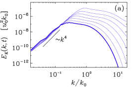
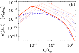
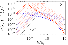
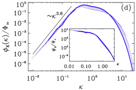
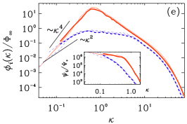
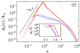
Figure 1: $E_{\rm K}(k,t)$ for different $t$ in HD DNS (a), compared with $E_{\rm M}$ (solid red) and $E_{\rm K}$ (dashed blue) in MHD without helicity (b), and with (c). Panels (d)–(f) show collapsed spectra using $\beta=3$ (d), $\beta=1$ (e), and $\beta=0$ (f).

In this Letter, we argue that the scaling exponent $q$ is not primarily determined by the initial value of $\alpha$, as suggested by Eq. (3), but by the physical processes involved. Moreover, we relax the restriction $\psi^{\prime}(0)=0$ and write instead

$$E(k\xi(t),t)=\xi^{-\beta}\phi(k\xi),$$ (4)

where $\xi=\xi(t)$ is computed from Eq. (1), and $\beta$ needs to be determined empirically or theoretically. Clearly, the initial powerlaw slope at small $k$ is no longer an adjustable input parameter, but is fixed by the form of $\phi=\phi(\kappa)$. Specifically, the “intrinsic” slope is $\alpha_{\ast}\equiv d\ln\phi/d\ln\kappa$. Evidently, $\psi$ can be computed from $\phi$ as $\psi(\kappa)=\xi^{\alpha-\beta}\phi(\kappa)/\kappa^{\alpha}$, but, in general, $d\ln\psi/d\ln\kappa=\alpha_{\ast}-\alpha\neq 0$ for $\kappa\to 0$.

In the following, we study examples of different decay behaviors in the diagnostic $pq$ diagram using data from DNS. As in earlier work TKBK12 , we solve the nonideal HD and MHD equations for an isothermal equation of state, i.e., pressure $P$ and density $\rho$ are proportional to each other, $P=\rho c_{\rm s}^{2}$, where $c_{\rm s}={\rm const}{}$ is the sound speed. The kinematic viscosity $\nu$ is characterized by the Reynolds number, $\mbox{\rm Re}=u_{\rm rms}\xi/\nu$, with $u_{\rm rms}=(2{\cal E})^{1/2}$ and the magnetic diffusivity $\eta$ is characterized by the magnetic Prandtl number $\mbox{\rm Pr}_{\rm M}=\nu/\eta$. The governing equations are solved using the Pencil Code PC ; suppl . The resolution is either $1152^{3}$ or $2304^{3}$ meshpoints. The Mach number $u_{\rm rms}/c_{\rm s}$ is always below unity, so compressibility effects are weak.

We first consider cases that have $\alpha=4$ for the initial spectral slopes of $E_{\rm K}$ or $E_{\rm M}$. We consider (i) HD decay, (ii) nonhelical MHD decay, and (iii) helical MHD decay. In cases (ii) and (iii), the magnetic energy also drives kinetic energy through the Lorentz force. The particular simulation of case (ii) was already presented in Ref. BKT15 , where inverse transfer to smaller wavenumbers was found in the absence of magnetic helicity using high-resolution DNS. Case (iii) leads to standard inverse transfer PFL76 ; BM99 ; CHB01 ; BJ04 . The resulting spectra are plotted in Figs. 1(a)–(c), where we show energy spectra for cases (i)–(iii) at different times. The values of Re at half time are roughly $100$, $230$, and $300$, respectively.

In Figs. 1(d)–(f) we compare with suitably compensated spectra. We compensate for the shift in $k$ by plotting $E(k,t)$ against $k\xi(t)$. The peak in each spectrum, which is approximately at $k=\xi^{-1}$, has then always the same position on the abscissa. Furthermore, to compensate for the decay in energy, we multiply $E$ by $\xi^{\beta}$ with some exponent $\beta$ such that the compensated spectra collapse onto a single function $\phi(k\xi(t))\approx\xi^{\beta}E(k\xi(t),t)$. In terms of the energy ${\cal E}(t)\equiv\int E(k,t)\,dk$, the function $\Phi=\xi^{\beta+1}{\cal E}_{\rm K}$ is asymptotically constant, $\Phi(t)\to\Phi_{\infty}$, and has the same dimension as $\phi$, so we plot the nondimensional ratio $\phi/\Phi_{\infty}$. The function $\psi(\kappa)$ is shown as an inset and normalized by $\Psi_{\ast}\equiv\xi^{\alpha-\beta}\Phi$ at the last time.

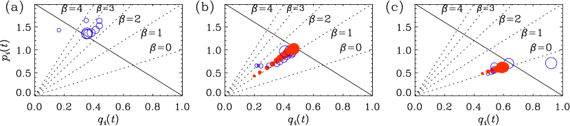
Figure 2: $pq$ diagrams for cases (i)–(iii). Open (closed) symbols correspond to $i={\rm K}$ (${\rm M}$) and their sizes increase with time.

Let us now consider solutions (i)–(iii) in the $pq$ diagram; see Figs. 2(a)–(c). These are compatible with independently computed $\beta q$ diagrams suppl . To study the relation between the exponents $\beta$ and $q$, we make use of Olesen’s scaling arguments and that $\phi$ is invariant under rescaling, to show from Eq. (4) that $\beta+3-2/q=0$, i.e.,

$$\beta=2/q-3,$$ (5)

or $q=2/(3+\beta)$. This is formally equivalent to Olesen’s relation (3), but with $\alpha$ being replaced by $\beta$. Moreover, unlike the exponent $\alpha$ in Eq. (2), the exponent $\beta$ in Eq. (4) bears no relation with the initial spectral slope, except for certain cases discussed below. The temporal decay of kinetic and magnetic energies follows power laws ${\cal E}_{i}(t)\sim t^{-p_{i}}$ for $i={\rm K}$ or ${\rm M}$. The exponents are obtained by integrating over $k$, ${\cal E}(t)=\xi^{-(\beta+1)}\int\phi\,d(k\xi)\propto t^{-p}$, and since $\xi\propto t^{q}$, this yields

$$p=(1+\beta)\,q.$$ (6)

Thus, in a $pq$ diagram, a certain value of $\beta$ corresponds to a line $p(t)\propto q(t)$ with the slope $\beta+1$. Furthermore, inserting Eq. (5) yields the line $p=2(1-q)$. We call this the self-similarity line.

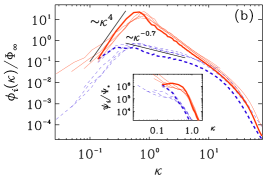
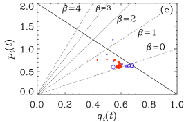
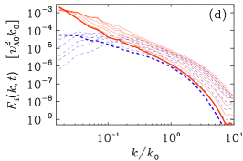
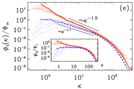
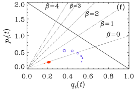
Figure 3: $E_{\rm M}$ (solid) and $E_{\rm K}$ (dashed) in MHD with fractional helicity and $\alpha=2$ (a), as well as full helicity and $\alpha=-1$ (d), together with compensated spectra (b,e) and the $pq$ diagrams (c,f).

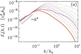
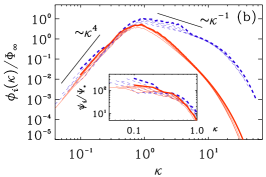
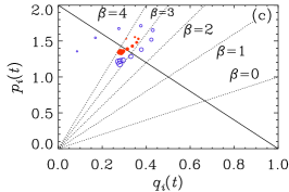
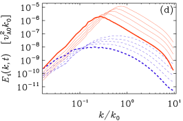
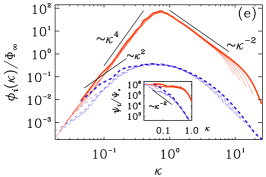
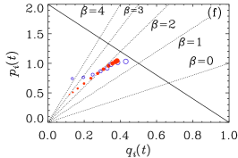
Figure 4: Similar to Fig. 3, but for nonhelical MHD with $\mbox{\rm Pr}_{\rm M}=0.01$ (a) and $\mbox{\rm Pr}_{\rm M}=100$ (d), together with compensated spectra (b,e) and the $pq$ diagrams (c,f).

Table 1: Scaling exponents and relation to physical invariants and their dimensions.

$\beta$ $p\quad\quad$ $q\quad\quad\;$    inv. dim. 4 $\quad 10/7\approx 1.43$ $\quad 2/7\approx 0.286$ $\quad{\cal L}$ $[x]^{7}[t]^{-2}$ 3 $8/6\approx 1.33$ $2/6\approx 0.333$ 2 $6/5=1.20$ $2/5=0.400$ 1 $4/4=1.00$ $2/4=0.500$ $\quad\langle\bm{A}_{\rm 2D}^{2}\rangle$ $[x]^{4}[t]^{-2}$ 0 $2/3\approx 0.67$ $2/3\approx 0.667$ $\quad\langle\bm{A}\cdot\bm{B}\rangle$ $[x]^{3}[t]^{-2}$ $-1$ $0/2=0.00$ $2/1=1.000$

The exponents $\beta$, $p$, and $q$ are roughly consistent with those expected based on the dimensions of potentially conserved quantities such as the Loitsiansky integral Dav10 , ${\cal L}=\int\bm{r}^{2}\langle\bm{u}(\bm{x})\cdot\bm{u}(\bm{x}+\bm{r})\rangle\,d\bm{r}\propto\ell^{5}u_{\ell}^{2}$, with typical velocity $u_{\ell}$ on scale $\ell$, the magnetic helicity, $\langle\bm{A}\cdot\bm{B}\rangle$, where $\bm{B}=\mbox{\boldmath$\nabla$}{}\times\bm{A}$ is the magnetic field in terms of the vector potential $\bm{A}$, and the mean squared vector potential, $\langle\bm{A}^{2}\rangle$, which is conserved in two-dimensions (2D); see Table LABEL:TSum.

In the HD case (i), the solution approaches the $\beta=3$ line and then settles on the self-similarity line at $q\approx 1/3$; see Fig. 2(a). This decay behavior departs from what would be expected if the Loitsiansky integral were conserved, i.e., $q=2/7$ and $\beta=4$. A slower decay law with $p=6/5$, corresponding to $q=2/5$ and $\beta=2$ has been favored by Saffman Saf67 , while experiments and simulations suggest $p=5/4$ Kang ; HB04 .

In case (ii), the solution evolves along $\beta=1$ toward $q=1/2$; see Figs. 2(b) and (e). This is compatible with the conservation of $\langle\bm{A}_{\rm 2D}^{2}\rangle$, where $\bm{A}_{\rm 2D}$ is the component of $\bm{A}$ which describes the 2D magnetic field in the plane perpendicular to the local intermediate eigenvector of the rate-of-strain matrix ${\sf S}$; see the supplemental material of BKT15 for details, and also Ole15 . The motivation for applying 2D arguments to 3D comes from the fact that for sufficiently strong magnetic fields the dynamics tends to become locally 2D in the plane perpendicular to the local field. This allows one to compute $\bm{A}$ in a gauge that projects out contributions perpendicular to the intermediate eigenvector of ${\sf S}$.

In case (iii) the solution evolves along $\beta=0$ toward $q=2/3$; see Figs. 2(c) and (f). This means that the spectrum shifts just in $k$, while the amplitude of $E_{\rm M}$ does not change, as can be seen from Fig. 1(c). This is consistent with the invariance of $\langle\bm{A}\cdot\bm{B}\rangle$; see Ref. BM99 .

Next, we investigate cases with $\alpha<4$. In the helical case with $\alpha=2$ we see that the subinertial range spectrum quickly steepens and approaches $\alpha_{\ast}=4\neq\alpha$; see Figs. 3(a)–(c). For $\alpha=-1$, which is a scale-invariant spectrum, the spectral energy remains nearly unchanged at small $k$, but the magnetic energy still decays due to decay at all higher $k$; see Figs. 3(d)–(f). The values of $p_{\rm M}$ and $q_{\rm M}$ are rather small ($\approx 0.2$), but the spectra can still be collapsed onto each other with $\beta=0$; see Fig. 3(e).

The examples discussed above demonstrate that in general $\beta\neq\alpha\neq\alpha_{\ast}$, i.e., the self-similarity parameter $\beta$ is not determined by the initial power spectrum but rather by the different physical processes involved. In helical MHD, we always find $\alpha_{\ast}=4$ together with $\beta=0$. For nonhelical MHD with $\alpha=4$ and $E_{\rm K}\propto k^{2}$, we find $\beta=1$, while in HD with $\alpha=4$, we find $\beta=3$. In agreement with earlier work YHB04 , the following exceptions can be identified: in HD with $1\leq\alpha\leq 3$ and in nonhelical MHD with $1\leq\alpha\leq$ we find $\beta=\alpha$ suppl . The only case where $\alpha=\beta=4$ has been found is when the magnetic Prandtl number $\mbox{\rm Pr}_{\rm M}\equiv\nu/\eta$ is small; see Figs. 4(a) and (c) for $\mbox{\rm Pr}_{\rm M}=0.01$. Here, the conservation of ${\cal L}$ may actually apply Dav10 . For $\mbox{\rm Pr}_{\rm M}\equiv\nu/\eta\gg 1$, on the other hand, we find $\beta=2$ scaling, even though $\alpha=4$; see Figs. 4(d) and (f).

In conclusion, the present work has revealed robust properties of the scaling exponent $\beta$ governing the time-dependence of the energy spectrum $E(k,t)$ through $\xi^{\beta}\phi(k\xi)$ with a time-independent scaling function $\phi$ and a time-dependent integral scale $\xi(t)$. The helical case is particularly robust in that any point in the $pq$ plane evolves along the $\beta=0$ line ($p=q$) toward the point $p=q=2/3$. Furthermore, if the initial spectrum has $\alpha=2$, it first steepens to $\alpha=4$ and then follows the same decay as with an initial $\alpha=4$. Moreover, for a scale-invariant spectrum with $\alpha=-1$, we again find $\beta=0$, i.e., the same as for $\alpha=2$ and 4, but now with $p_{\rm M}\approx q_{\rm M}\approx 0.2$; see Fig. 3(f). In the fractionally helical case, points in the $pq$ plane evolve toward the $\beta=0$ line and, for $\alpha\geq 2$, later toward $p_{\rm M}=q_{\rm M}=2/3$.

Our results have consequences for two types of cosmological initial magnetic fields: causal ones with $E_{\rm M}\propto k^{4}$ will always be accompanied by a shallower kinetic energy spectrum $E_{\rm K}\propto k^{2}$, thus favoring inverse transfer BKT15 ; KTBN13 , while a scale-invariant inflation-generated helical field exhibits self-similarity with $\beta=0$ in the same way as for other initial slopes, but now with $p=q\approx 0.2$ instead of $2/3$. For decaying wind tunnel turbulence, Loitsiansky scaling is ruled out in favor of Saffman scaling, provided $\alpha=2$. No inverse transfer is possible in HD, even if $\alpha=4$, contrary to earlier claims Ole97 . The experimental realization of initial conditions with $\alpha\neq 2$ could be challenging for wind tunnels, but may well be possible in plasma experiments Forest15 .

Supplemental Material

to “Classes of hydrodynamic and magnetohydrodynamic turbulent decay” (arXiv:1607.01360)

by A. Brandenburg & T. Kahniashvili

I Effect of phase errors

By default, the Pencil Code uses sixth order accurate finite difference representations for the first and second derivatives. A low spatial order of the scheme implies that at high wavenumbers the magnitude of the numerical derivative is reduced, leading to lower advection speeds of the high wavenumber Fourier components. This is generally referred to as phase error. Thus, for an advected tophat function, the high wavenumber constituents will lag behind, creating the well-known Gibbs phenomenon which needs to be controlled by a certain amount of viscosity. Higher order schemes require less viscosity to control the Gibbs phenomenon (BD02, ). On the other hand, any turbulence simulation requires a sufficient amount of viscosity to dissipate kinetic energy. It is therefore thought that for a sixth orders scheme the two limits on the viscosity are similar and that it is not advantageous to use higher order representations of the spatial derivatives.

Table 2: Coefficients $c_{j}^{(n)}\equiv a_{j}^{(n)}/b^{(n)}$

$N$ $n$ $b^{(n)}$ $a_{0}^{(n)}$ $a_{1}^{(n)}$ $a_{2}^{(n)}$ $a_{3}^{(n)}$ $a_{4}^{(n)}$ $a_{5}^{(n)}$ 10 1 2520 0 2100 $-600$ 150 $-25$ 2 8 1 840 0 672 $-168$ 32 $-3$ 6 1 60 0 45 $-9$ 1 4 1 12 0 8 $-1$ 2 1 2 0 1 10 2 25200 $-73766$ 42000 $-6000$ $1000$ $-125$ $8$ 8 2 5040 $-14350$ 8064 $-1008$ $128$ $-9$ 6 2 180 $-490$ 270 $-27$ $2$ 4 2 12 $-30$ 16 $-1$ 2 2 1 $-2$ 1

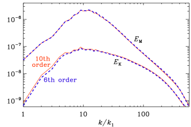
Figure 5: Magnetic (upper curves) and kinetic (lower curves) energy spectra for at $t=110$ for the sixth order (blue, dashed) and tenth order (red, solid) finite difference schemes.

To verify this in the present context, we have run a high Reynolds number case both with sixth and tenth order schemes. In the Pencil Code, the order of the scheme can easily be changed by setting DERIV=deriv_10th. In that case, first and second derivatives are represented as

$${\rm d}^{n}f_{i}/{\rm d}x^{n}=\sum_{j=-N}^{N}({\rm sgn}j)^{n}c_{|j|}^{(n)}f_{i+j}/\delta x^{n},$$ (7)

with coefficient $c_{j}^{(n)}$ given in Table LABEL:Tcoeff for schemes of order $N$. The result of the comparison is shown in Fig. 5. The differences between the two cases are negligible, except that with the more accurate tenth order scheme the inverse transfer of kinetic energy to larger scales is now slightly stronger. This is consistent with our earlier findings that the inverse transfer in nonhelical MHD becomes more pronounced at larger resolution.

II Isothermal versus polytropic equation of state

An isothermal equation of state is often used in subsonic compressible turbulence to approximate the conditions of nearly incompressible flows. Using instead a polytropic equation of state means that in the momentum equation the pressure gradient term for an isothermal gas is amended by a factor $\propto\rho^{\gamma-1}$, i.e.,

$$c_{\rm s}^{2}\mbox{\boldmath$\nabla$}{}\ln\rho\to c_{\rm s0}^{2}\left({\rho\over\rho_{0}}\right)^{\gamma-1}\mbox{\boldmath$\nabla$}{}\ln\rho,$$ (8)

where $\gamma=5/3$ is the polytropic index for a monatomic gas instead of $\gamma\to 1$ for an isothermal gas. Using $\gamma=5/3$ implies a slightly stiffer equation of state, so one has to drive stronger to achieve the same compression; see Sect. 9.3.6 of Bra03 . In the present context of subsonic decaying turbulence, this leads to slightly smaller vorticity fluctuations, as is shown in Fig. 6. It is seen that the difference between $\gamma=5/3$ and 1 is negligible for all practical purposes.

Figure 6: Difference in rms vorticity, $\omega_{\rm rms}$, between the isothermal and polytropic solutions.

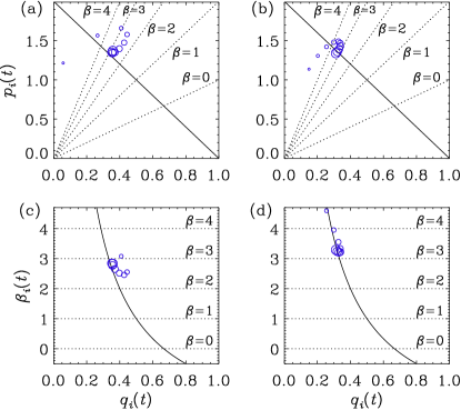
Figure 7: $pq$ diagrams for hydrodynamic turbulence with $\nu={\rm const}{}$ (a) and time-dependent $\nu(t)\propto t^{r}$ (b) with $r=-0.43$ and $\alpha=4$. Panels (c) and (d) show the corresponding $\beta q$ diagrams. Open (closed) symbols corresponds to $i={\rm K}$ (${\rm M}$) and their sizes increase with time.

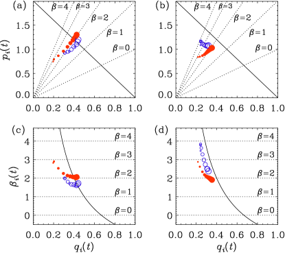
Figure 8: Similar to Fig. 7, but for nonhelical MHD turbulence with $\nu=\eta={\rm const}{}$ (a) and time-dependent $\nu(t)=\eta(t)\propto t^{r}$ (b) with $r=-0.43$ and $\alpha=4$.

III Time-dependent $\nu(t)$ and $\eta(t)$

Table 3: Exponents $r$ for different $\alpha$.

$\alpha$ 0 $1\quad$ 2 3 4 $r$ $\quad 0.33\quad$ $0\quad$ $-0.20\quad$ $-0.33\quad$ $-0.43\quad$

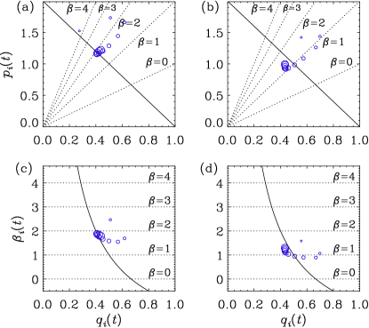
Figure 9: Similar to Fig. 7, but for $\alpha=2$ (a) and $\alpha=1$ (b) with $\nu={\rm const}{}$.

As pointed out by Olesen Ole97 , the hydrodynamic and MHD equations are invariant under rescaling $x\to\tilde{x}\ell$ and $t\to\tilde{t}\ell^{1/q}$ provided also $\nu$ and $\eta$ are being dynamically rescaled such that

$$\nu(t)=\nu_{0}\,\max(t/t_{0},1)^{r},\quad\eta(t)=\eta_{0}\,\max(t/t_{0},1)^{r},$$ (9)

with

$$r=2q-1=(1-\alpha)/(3+\alpha);$$ (10)

see Table LABEL:TRofAlp. The use of the $\max$ function in Eq. (9) limits the values of $\nu\leq\nu_{0}$ and $\eta\leq\eta_{0}$ for $t\leq t_{0}$ when $r<0$. At large Reynolds numbers, the time-dependence is not expected to be important. To verify this, we compare in Fig. 7 hydrodynamic runs with constant and time-dependent $\nu$ using $\alpha=4$. Both cases are similar and the case with time-dependent $\nu$ still has $\beta=3\neq\alpha$. Similar behavior is found in MHD; see Fig. 8, where we compare runs with constant and time-dependent $\nu$ and $\eta$ using again $\alpha=4$. In both cases, we find $\beta=2\neq\alpha$.

In agreement with earlier work we find that in hydrodynamic cases with $\alpha=2$ and $\alpha=1$, we have $\beta=\alpha$ YHB04 . This is demonstrated in Fig. 9, where we show the $pq$ and $\beta q$ diagrams for these two cases.