Hamiltonian Approach to Internal Wave-Current Interactions in a Two-Media Fluid with a Rigid Lid

Abstract

We examine a two-media 2-dimensional fluid system consisting of a lower medium bounded underneath by a flatbed and an upper medium with a free surface with wind generated surface waves but considered bounded above by a lid by an assumption that surface waves have negligible amplitude. An internal wave driven by gravity which propagates in the positive $x$-direction acts as a free common interface between the media. The current is such that it is zero at the flatbed but a negative constant, due to an assumption that surface winds blow in the negative $x$-direction, at the lid. We are concerned with the layers adjacent to the internal wave in which there exists a depth dependent current for which there is a greater underlying than overlying current. Both media are considered incompressible and having non-zero constant vorticities. The governing equations are written in canonical Hamiltonian form in terms of the variables, associated to the wave (in a presence of a constant current). The resultant equations of motion show that wave-current interaction is influenced only by the current profile in the ’strip’ adjacent to the internal wave.

2010 Mathematics Subject Classification: 35Q35, 37K05, 74J30.

Key words: Internal waves, vorticity, current, shear flow, Hamiltonian system.

1 Introduction

Studies of internal waves, such as sharp temperature gradients called thermoclines which separate oceanic bodies of water which are at different temperatures, are of significant interest to climatologists, marine biologists, coastal engineers, etc.

The study of internal waves draws from previous single medium irrotational [1], [2], [3], [4], [5], [6] and rotational [7], [8], [9], [10], [11], [12], [13], [14] studies and from appropriate studies of 2-media systems such as [15], [16], [17], [18]. However, these studies need to be extended to include the interaction between waves and currents.

Recent studies include the interaction between waves that propagate across the Pacific Ocean and the Equatorial Undercurrent (EUC) [19], a Hamiltonian formulation describing the 2-dimensional nonlinear interaction between coupled surface waves, internal waves, and an underlying current with piecewise constant vorticity, in a two-layered fluid overlying a flat bed [20] and using shifted variables to transform a non-canonical wave-current system into a canonical system which has zero vorticity in the layers adjacent to the internal wave [21]. This study aims to provide a Hamiltonian formulation of a two-media bounded system which is rotational in the layers adjacent to the internal wave and hence show that wave-current interaction is influenced only by the current profile in this ’strip’.

2 Preliminaries

The system under study consists of a 2-dimensional internal wave under the restorative action of gravity, which acts as a free common interface separating two fluid media, and a depth dependent current as per Figure 1.

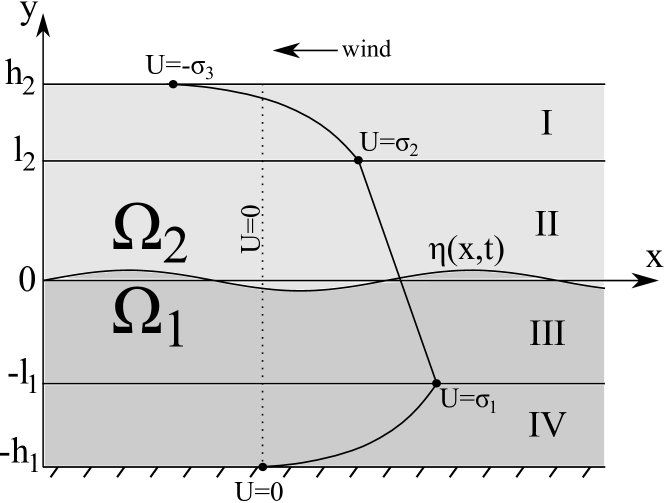
Figure 1: System setup. The current profile in layers I and IV is arbitrary as we are only concerned with layers II and III as the internal wave is a free interface between these layers. Continuity of $U(y)$ is assumed in layers I and IV.

The medium underneath the internal wave is defined by the domain $\Omega_{1}=\{(x,y)\in\mathbb{R}^{2}:-h_{1}<y<\eta(x,t)\}$. This medium is bounded at the bottom by an impermeable flatbed at a depth $-h_{1}$. The medium above the internal wave is defined by the domain $\Omega_{2}=\{(x,y)\in\mathbb{R}^{2}:\eta(x,t)<y<h_{2}\}$. This medium is regarded as being bounded on top by an impermeable lid at a height $h_{2}$, but in reality is a free surface with negligible wave amplitude. Throughout the article the subscript $1$ will be used to mean evaluation for the lower medium $\Omega_{1}$, subscript $2$ means evaluation for the upper medium $\Omega_{2}$, subscript $i=\{1,2\}$ means evaluation for both media and subscript $c$ will be used to denote evaluation at the common interface. Non-lateral velocity flow is described by ${\bf{V}}_{i}(x,y,z)=(u_{i},v_{i},0)$. The arbitrary periodic function $\eta(x,t)$ describes the elevation of the internal wave, i.e. $y=\eta$ is the equation of the internal wave. We define the mean of $\eta$ to be the shear surface at $y=0$ with the centre of gravity in the negative $y$-direction.

A depth dependent current $U_{1}(y)$ flows in $\Omega_{1}$ and, correspondingly, $U_{2}(y)$ flows in $\Omega_{2}$. Currents are described for the system under study via the continuous function $U_{i}(y)$ as

(1) $$U_{i}(y)=\left\{\begin{array}[]{lcl}-\sigma_{3},\qquad y=h_{2}\mbox{ (lid)}\\ \sigma_{2},\qquad y=l_{2}\\ \gamma y+\kappa,\qquad l_{2}\geq y\geq-l_{1}\mbox{ (layers II and III)}\\ \sigma_{1},\qquad y=-l_{1}\\ 0,\qquad y=-h_{1}\mbox{ (flatbed)}\end{array}\right.$$

for the positive constants $\sigma_{1}$, $\sigma_{2}$, $\sigma_{3}$, $\kappa$, $l_{i}$, $h_{i}$, $\gamma$ and $\kappa$, where $\kappa$ is the velocity of the time-independent current at $y=0$ and $\gamma$ is the non-zero constant vorticity for layers II and III, noting that the current is arbitrary in layers I and IV (however represented by a continuous function everywhere).

We consider a velocity field which is defined by:

(2) $$\left\{\begin{array}[]{lcl}u_{i}=\tilde{\varphi}_{i,x}+U_{i}(y)\\ v_{i}={\tilde{\varphi}}_{i,y}.\end{array}\right.$$

We have separated the wave and current contributions to the velocity and so we define ${\tilde{\varphi}}_{i}$ as the wave velocity potential for $\Omega_{i}$ and in particular the velocity components in layers II and III are [22]

(3) $$\left\{\begin{array}[]{lcl}u_{i}=\tilde{\varphi}_{i,x}+\gamma y+\kappa\\ v_{i}={\tilde{\varphi}}_{i,y}.\end{array}\right.$$

Additionally, the stream function $\psi_{i}$ is introduced, defined by:

(4) $$\left\{\begin{array}[]{lcl}u_{i}=\psi_{i,y}\\ v_{i}=-\psi_{i,x}.\end{array}\right.$$

$\rho_{1}$ and $\rho_{2}$ are the respective constant densities of the lower and upper media and stability is given by the immiscibility condition

(5) $$\rho_{1}>\rho_{2}.$$

The rotationality of the layers II and III is given by the condition

(6) $$\gamma<0\Leftrightarrow\sigma_{1}>\sigma_{2}$$

ensuring non-zero vorticity in this region. Alternatively $\sigma_{2}>\sigma_{1}$ could also be considered for $\gamma>0$.

We assume that for large $|x|$ the amplitude of $\eta$ attenuates and hence make the following assumptions

(7) $$\lim_{|x|\rightarrow\infty}\eta(x,t)=0,$$

(8) $$\lim_{|x|\rightarrow\infty}{\tilde{\varphi}}_{i}(x,y,t)=0,$$

and

(9) $$-l_{1}<\eta(x,t)<l_{2}\mbox{ for all $x$ and $t$},$$

i.e. the wave is localised in the strip.

We have the following equation (Euler’s equation)

(10) $$\nabla\Big{(}(\varphi_{i,t})_{c}+\frac{1}{2}(\nabla\psi_{i})_{c}^{2}-\gamma\psi_{i}\Big{)}=\nabla\Big{(}-\frac{p_{i}}{\rho_{1}}-g\eta\Big{)}$$

where $p_{i}$ is the dynamic pressure, $g$ is the acceleration due to gravity (where $y$ points in the opposite direction to the center of gravity) and $\nabla=(\partial_{x},\partial_{y})$. The following Bernoulli condition (cf. [18]) at the interface follows from Euler’s equation and assumptions (7) and (8):

(11) $$\rho_{1}\Big{(}(\varphi_{1,t})_{c}+\frac{1}{2}(\nabla\psi_{1})_{c}^{2}-\gamma\chi_{1}+g\eta\Big{)}=\rho_{2}\Big{(}(\varphi_{2,t})_{c}+\frac{1}{2}(\nabla\psi_{2})_{c}^{2}-\gamma\chi_{2}+g\eta\Big{)}+f(t)$$

where $\chi_{i}$ is the stream function evaluated at the interface. Since the two media do not mix, $\chi_{1}=\chi_{2}\equiv\chi$. Moreover, $f(t)$ is an arbitrary function of time and depends on how the potentials are defined at $\pm\infty$. Clearly such a function can be absorbed in the definition of the wave potentials, but we will keep it separate for further convenience. We know by comparing (3) and (4) that

(12) $$\frac{1}{2}(\nabla\psi_{i})_{c}^{2}=\frac{1}{2}({\tilde{\varphi}}_{i,x})_{c}^{2}+\frac{1}{2}({\tilde{\varphi}}_{i,y})_{c}^{2}+\frac{1}{2}(\gamma\eta+\kappa)^{2}+(\tilde{\varphi}_{i,x})_{c}\gamma\eta+\kappa(\tilde{\varphi}_{i,x})_{c}$$

and hence we can express the Bernoulli condition in terms of wave and current components only as

(13) $$(\rho_{1}{\tilde{\varphi}}_{1,t}-\rho_{2}{\tilde{\varphi}}_{2,t})_{c}+\kappa(\rho_{1}\tilde{\varphi}_{1,x}-\rho_{2}\tilde{\varphi}_{2,x})_{c}+\frac{\rho_{1}}{2}|\nabla{\tilde{\varphi}}_{1}|_{c}^{2}-\frac{\rho_{2}}{2}|\nabla{\tilde{\varphi}}_{2}|_{c}^{2}\\ +\frac{1}{2}(\rho_{1}-\rho_{2})(\gamma\eta+\kappa)^{2}+\gamma\eta(\rho_{1}\tilde{\varphi}_{1,x}-\rho_{2}\tilde{\varphi}_{2,x})_{c}\\ -(\rho_{1}-\rho_{2})\gamma\chi+(\rho_{1}-\rho_{2})g\eta=f(t).$$

The terms with $\gamma$ and $\kappa$ are due to the wave-current interaction. For example, the second term is due to overall translation leading to a shift $\partial_{t}\rightarrow\partial_{t}+\kappa\partial_{x}$. The equation suggests the introduction of the variable

(14) $$\xi:=\rho_{1}\xi_{1}-\rho_{2}\xi_{2},$$

where

(15) $$\xi_{i}:=(\tilde{\varphi}_{i})_{c}=\tilde{\varphi}_{i}(x,\,\eta(x,\,t),\,t).$$

We also have the following kinematic boundary conditions at the interface, using the velocity representations (3)

(16) $$\left\{\begin{array}[]{lcl}\eta_{t}+\eta_{x}\big{(}\gamma\eta+(\tilde{\varphi}_{i,x})_{c}+\kappa\big{)}+(\tilde{\varphi}_{i,y})_{c}=0\\ (\tilde{\varphi}_{1,y})_{b}=(\tilde{\varphi}_{2,y})_{l}=0\end{array}\right.$$

noting that ${\bf{V_{1}}}(x,-h_{1},0)=(u_{1},0,0)$ and ${\bf{V_{2}}}(x,h_{2},0)=(u_{2},0,0)$, where the subscripts $b$ and $l$ denote evaluation at the bottom (lower boundary) and lid (upper boundary) respectively.

3 Hamiltonian Formulation

If we consider the system under study as an irrotational system the Hamiltonian, $H$, is given by the sum of the kinetic and potential energies as:

(17) $$H=\frac{\rho_{1}}{2}\int\limits_{\mathbb{R}}\int\limits_{-h_{1}}^{\eta}(u_{1}^{2}+v_{1}^{2})dydx+\frac{\rho_{2}}{2}\int\limits_{\mathbb{R}}\int\limits_{\eta}^{h_{2}}(u_{2}^{2}+v_{2}^{2})dydx+\frac{1}{2}(\rho_{1}-\rho_{2})\int\limits_{\mathbb{R}}g\eta^{2}dx.$$

The kinetic energy term for $\Omega_{1}$ is

(18) $$K_{1}=\frac{\rho_{1}}{2}\int\limits_{\mathbb{R}}\int\limits_{-h_{1}}^{\eta}(u_{1}^{2}+v_{1}^{2})dydx$$

which we can split into layers IV and III, respectively, as

(19) $$K_{1}=\frac{\rho_{1}}{2}\int\limits_{\mathbb{R}}\int\limits_{-h_{1}}^{-l_{1}}(u_{1}^{2}+v_{1}^{2})dydx+\frac{\rho_{1}}{2}\int\limits_{\mathbb{R}}\int\limits_{-l_{1}}^{\eta}(u_{1}^{2}+v_{1}^{2})dydx.$$

For layer IV the kinetic energy is

(20) $$\frac{\rho_{1}}{2}\int\limits_{\mathbb{R}}\int\limits_{-h_{1}}^{-l_{1}}(u_{1}^{2}+v_{1}^{2})dydx=\frac{\rho_{1}}{2}\int\limits_{\mathbb{R}}\int\limits_{-h_{1}}^{-l_{1}}({\tilde{\varphi}}_{1,x})^{2}dydx+\frac{\rho_{1}}{2}\int\limits_{\mathbb{R}}\int\limits_{-h_{1}}^{-l_{1}}({\tilde{\varphi}}_{1,y})^{2}dydx\\ +\frac{\rho_{1}}{2}\int\limits_{\mathbb{R}}\int\limits_{-h_{1}}^{-l_{1}}\gamma^{2}y^{2}dydx+\frac{\rho_{1}}{2}\int\limits_{\mathbb{R}}\int\limits_{-h_{1}}^{-l_{1}}U_{1}^{2}dydx+\rho_{1}\int\limits_{\mathbb{R}}\int\limits_{-h_{1}}^{-l_{1}}\tilde{\varphi}_{1,x}\gamma ydydx\\ +\rho_{1}\int\limits_{\mathbb{R}}\int\limits_{-h_{1}}^{-l_{1}}\gamma U_{1}ydydx+\rho_{1}\int\limits_{\mathbb{R}}\int\limits_{-h_{1}}^{-l_{1}}U_{1}\tilde{\varphi}_{1,x}dydx.$$

However, terms 3-7 combine to produce a constant which is irrelevant in terms of dynamic considerations (does not contribute to the variations with respect to the field variables). Moreover $\int\limits_{\mathbb{R}}\eta(x^{\prime},t)dx^{\prime}=0$ (the mean deviation is by definition zero) and the fields vanish at $x=\pm\infty$ so that integration of total $x-$ derivatives produces zero, thus

(21) $$\frac{\rho_{1}}{2}\int\limits_{\mathbb{R}}\int\limits_{-h_{1}}^{-l_{1}}(u_{1}^{2}+v_{1}^{2})dydx=\frac{\rho_{1}}{2}\int\limits_{\mathbb{R}}\int\limits_{-h_{1}}^{-l_{1}}({\tilde{\varphi}}_{1,x})^{2}dydx+\frac{\rho_{1}}{2}\int\limits_{\mathbb{R}}\int\limits_{-h_{1}}^{-l_{1}}({\tilde{\varphi}}_{1,y})^{2}dydx.$$

For layer III the kinetic energy is

(22) $$\frac{\rho_{1}}{2}\int\limits_{\mathbb{R}}\int\limits_{-l_{1}}^{\eta}(u_{1}^{2}+v_{1}^{2})dydx=\frac{\rho_{1}}{2}\int\limits_{\mathbb{R}}\int\limits_{-l_{1}}^{\eta}({\tilde{\varphi}}_{1,x})^{2}dydx+\frac{\rho_{1}}{2}\int\limits_{\mathbb{R}}\int\limits_{-l_{1}}^{\eta}({\tilde{\varphi}}_{1,y})^{2}dydx\\ +\frac{\rho_{1}}{2}\int\limits_{\mathbb{R}}\int\limits_{-l_{1}}^{\eta}(\gamma y+\kappa)^{2}dydx+\rho_{1}\int\limits_{\mathbb{R}}\int\limits_{-l_{1}}^{\eta}\tilde{\varphi}_{1,x}\gamma ydydx+\rho_{1}\int\limits_{\mathbb{R}}\int\limits_{-l_{1}}^{\eta}\kappa\tilde{\varphi}_{1,x}dydx.$$

We write

(23) $$\frac{\rho_{1}}{2}\int\limits_{\mathbb{R}}\int\limits_{-l_{1}}^{\eta}(\gamma y+\kappa)^{2}dydx=\frac{\rho_{1}}{6\gamma}\int\limits_{\mathbb{R}}(\gamma\eta+\kappa)^{3}dx$$

noting that $\int\limits_{\mathbb{R}}(\gamma\eta+\kappa)^{3}dx$ can be properly re-normalised as $\int\limits_{\mathbb{R}}((\gamma\eta+\kappa)^{3}-\kappa^{3})dx$ as the variation in $\int\limits_{\mathbb{R}}\kappa^{3}dx$ is zero.

We introduce the Dirichlet-Neumann operator $G_{i}(\eta)$ (see [3], [16]) given by

(24) $$G_{i}(\eta)\xi_{i}=(\partial_{{{\bf{n}}_{i}}}\tilde{\varphi}_{i})\sqrt{1+(\eta_{x})^{2}},$$

where $\partial_{{{\bf{n}}_{i}}}\tilde{\varphi}_{i}$ is the normal derivative of the velocity potential $\tilde{\varphi}_{i}$, at the interface, for an outward normal ${{\bf{n}}_{i}}$, and also define [15]

(25) $$B:=\rho_{1}G_{2}(\eta)+\rho_{2}G_{1}(\eta).$$

Thus we can determine that

(28) $$\left\{\begin{array}[]{lcl}\xi_{1}=B^{-1}\big{(}G_{2}(\eta)\xi\big{)}\\ \xi_{2}=B^{-1}\big{(}-G_{1}(\eta)\xi\big{)}\end{array}\right.$$

The integral with $\rho_{1}\kappa\tilde{\varphi}_{1,x}$ term, using the Leibniz integral rule with varying limits (cf. [17]), can be written as

(29) $$\rho_{1}\int\limits_{\mathbb{R}}\int\limits_{-l_{1}}^{\eta}\kappa\tilde{\varphi}_{1,x}dydx=-\rho_{1}\kappa\int\limits_{\mathbb{R}}\xi_{1}\eta_{x}dx$$

and the $\rho_{1}\gamma y\tilde{\varphi}_{1,x}$ term as

(30) $$\rho_{1}\int\limits_{\mathbb{R}}\int\limits_{-h_{1}}^{\eta}\gamma y\tilde{\varphi}_{1,x}dydx =-\rho_{1}\int\limits_{\mathbb{R}}\gamma\xi_{1}\eta\eta_{x}dx$$

and hence we write the Hamiltonian for $\Omega_{1}$ as

(31) $$H_{1}=\frac{\rho_{1}}{2}\int\limits_{\mathbb{R}}\int\limits_{-h_{1}}^{\eta}|\nabla{\tilde{\varphi}}_{1}|^{2}dydx+\frac{\rho_{1}}{2}\int\limits_{\mathbb{R}}g\eta^{2}\,dx\\ +\frac{\rho_{1}}{6\gamma}\int\limits_{\mathbb{R}}(\gamma\eta+\kappa)^{3}dx-\rho_{1}\int\limits_{\mathbb{R}}\gamma\xi_{1}\eta\eta_{x}dx-\rho_{1}\kappa\int\limits_{\mathbb{R}}\xi_{1}\eta_{x}dx.$$

We follow the same procedure for $\Omega_{2}$ to obtain the corresponding energy as

(32) $$H_{2}=\frac{\rho_{2}}{2}\int\limits_{\mathbb{R}}\int\limits_{\eta}^{h_{2}}|\nabla{\tilde{\varphi}}_{2}|^{2}dydx-\frac{\rho_{2}}{2}\int\limits_{\mathbb{R}}g\eta^{2}dydx\\ -\frac{\rho_{2}}{6\gamma}\int\limits_{\mathbb{R}}(\gamma\eta+\kappa)^{3}dx+\rho_{2}\int\limits_{\mathbb{R}}\gamma\xi_{2}\eta\eta_{x}dx+\rho_{2}\kappa\int\limits_{\mathbb{R}}\xi_{2}\eta_{x}dx.$$

The total energy is therefore $H=H_{1}+H_{2}$ or in terms of ($\eta$, $\xi$)

(33) $$H(\eta,\xi)=\frac{1}{2}\int\limits_{\mathbb{R}}\xi\big{(}G_{1}(\eta)B^{-1}G_{2}(\eta)\big{)}\xi\,dx+\frac{\rho_{1}-\rho_{2}}{2}\int\limits_{\mathbb{R}}g\eta^{2}\,dx-\kappa\int\limits_{\mathbb{R}}\xi\eta_{x}dx\\ -\int\limits_{\mathbb{R}}\gamma\eta\eta_{x}\xi dx+\frac{(\rho_{1}-\rho_{2})}{6\gamma}\int\limits_{\mathbb{R}}(\gamma\eta+\kappa)^{3}dx.$$

Defining the Hamiltonian which has no current or vorticity components, $H_{0}$, as

(34) $$H_{0}(\eta,\xi)=\frac{1}{2}\int\limits_{\mathbb{R}}\xi\big{(}G_{1}(\eta)B^{-1}G_{2}(\eta)\big{)}\xi\,dx+(\rho_{1}-\rho_{2})\frac{1}{2}\int\limits_{\mathbb{R}}g\eta^{2}\,dx$$

we can write

(35) $$H(\eta,\xi)=H_{0}-\kappa\int\limits_{\mathbb{R}}\xi\eta_{x}dx-\int\limits_{\mathbb{R}}\gamma\eta\eta_{x}\xi dx+\frac{(\rho_{1}-\rho_{2})}{6\gamma}\int\limits_{\mathbb{R}}(\gamma\eta+\kappa)^{3}dx.$$

The equations of motion can be written in Hamiltonian form as follows. From (16) the dynamic boundary condition

$$\eta_{t} =-\gamma\eta\eta_{x}+(\tilde{\varphi}_{i,x})_{c}\eta_{x}-\kappa\eta_{x}-(\tilde{\varphi}_{i,y})_{c}$$

(36) $$=\delta_{\xi}H_{0}-\kappa\eta_{x}-\gamma\eta\eta_{x}=\delta_{\xi}H.$$

We note that the quantities in the Bernoulli condition (13) are

(37) $$\rho_{1}({\tilde{\varphi}_{1,x}})_{c}-\rho_{2}({\tilde{\varphi}_{2,x}})_{c} =\xi_{x}-(\rho_{1}{\tilde{\varphi}_{1,y}}-\rho_{2}{\tilde{\varphi}_{2,y}})_{c}\eta_{x}$$

(38) $$\rho_{1}({\tilde{\varphi}_{1,t}})_{c}-\rho_{2}({\tilde{\varphi}_{2,t}})_{c} =\xi_{t}-(\rho_{1}{\tilde{\varphi}_{1,y}}-\rho_{2}{\tilde{\varphi}_{2,y}})_{c}\eta_{t}.$$

and we can write it as

(39) $$\xi_{t}-(\rho_{1}{\tilde{\varphi}}_{1,y}-\rho_{2}{\tilde{\varphi}}_{2,y})_{c}(\eta_{t}+(\gamma\eta+\kappa)\eta_{x})+\frac{\rho_{1}}{2}|\nabla{\tilde{\varphi}}_{1}|_{c}^{2}-\frac{\rho_{2}}{2}|\nabla{\tilde{\varphi}}_{2}|_{c}^{2}\\ +(\gamma\eta+\kappa)\xi_{x}+\frac{1}{2}(\rho_{1}-\rho_{2})(\gamma\eta+\kappa)^{2}-(\rho_{1}-\rho_{2})\gamma\chi+(\rho_{1}-\rho_{2})g\eta=f(t).$$

or due to (3) as

(40) $$\xi_{t}-(\rho_{1}{\tilde{\varphi}}_{1,y}-\rho_{2}{\tilde{\varphi}}_{2,y})_{c}({\tilde{\varphi}}_{i,x}\eta_{x}-{\tilde{\varphi}}_{i,y})_{c}+\frac{\rho_{1}}{2}|\nabla{\tilde{\varphi}}_{1}|_{c}^{2}-\frac{\rho_{2}}{2}|\nabla{\tilde{\varphi}}_{2}|_{c}^{2}+(\rho_{1}-\rho_{2})g\eta\\ +(\gamma\eta+\kappa)\xi_{x}+\frac{1}{2}(\rho_{1}-\rho_{2})(\gamma\eta+\kappa)^{2}-(\rho_{1}-\rho_{2})\gamma\chi=f(t).$$

Noting the ’usual’, not related to the current terms,

(41) $$\xi_{t}+\delta_{\eta}H_{0}+(\gamma\eta+\kappa)\xi_{x}+\frac{1}{2}(\rho_{1}-\rho_{2})(\gamma\eta+\kappa)^{2}-(\rho_{1}-\rho_{2})\gamma\chi=f(t).$$

and finally, from (35)

(42) $$\xi_{t}+\delta_{\eta}H-(\rho_{1}-\rho_{2})\gamma\chi=f(t).$$

The equation for $\xi_{t}$ is given up to an arbitrary function of time because the Hamiltonian can always be ’renormalised’ by a term $-f(t)\int\limits_{\mathbb{R}}\eta dx$ which has a variation of $-f(t)$ with respect to $\eta$ but is otherwise zero by definition. Thus, for the renormalised Hamiltonian

(43) $$\xi_{t}=-\delta_{\eta}H+(\rho_{1}-\rho_{2})\gamma\chi.$$

Since $\chi=-\int_{-\infty}^{x}\eta_{t}(x^{\prime},t)dx^{\prime}=-\int_{-\infty}^{x}\delta_{\xi}Hdx^{\prime},$ after a change of variables [14] via the transformation $(\eta,\xi)\rightarrow(\eta,\zeta)$

(44) $$\xi\rightarrow\zeta=\xi-\frac{(\rho_{1}-\rho_{2})\gamma}{2}\int_{-\infty}^{x}\eta(x^{\prime},t)\,dx^{\prime}.$$

the system acquires a canonical Hamiltonian form:

(45) $$\left\{\begin{array}[]{lcl}\eta_{t}=\delta_{\zeta}H\\ \zeta_{t}=-\delta_{\eta}H\end{array}\right.$$

In conclusion we have shown that the wave-current is influenced only by the current profile in the ’strip’ (layers II and III), i.e. outside this region the continuous current is arbitrary.

4 Conclusion

The governing equations of a system of two-media, bounded on top by a lid and on the bottom by a flatbed, with an internal wave providing a free common interface and with a depth dependent current were written in a canonical Hamiltonian form in terms of the ’wave’-related variables $(\eta,\zeta).$

It was then shown that the wave-current interactions are influenced only by the current profile in the ’strip’, and do not depend on the current profile in the other layers.

Alan Compelli
School of Mathematical Sciences
Dublin Institute of Technology
Kevin Street, Dublin 8, Ireland

Rossen Ivanov
School of Mathematical Sciences
Dublin Institute of Technology
Kevin Street, Dublin 8, Ireland
email: rossen.ivanov@dit.ie
and
Faculty of Mathematics
Oskar-Morgenstern-Platz 1
University of Vienna
1090 Vienna, Austria

References

• [1] V. Zakharov. Stability of periodic waves of finite amplitude on the surface of a deep fluid. Zh. Prikl. Mekh. Tekh. Fiz. 9 (1968), 86–94.
• [2] T. Benjamin, P. Olver. Hamiltonian structure, symmetries and conservation laws for water waves. J. Fluid Mech. 125 (1982), 137–185.
• [3] W. Craig. Water waves, Hamiltonian systems and Cauchy integrals. IMA Vol. Math. Appl. 30 (1991), 37–45.
• [4] D. Milder. A note regarding ‘On Hamilton‘s principle for water waves‘. J. Fluid Mech. 83 (1977), 159–161.
• [5] J. Miles. Hamiltonian formulations for surface waves. Appl. Sci. Res. 37 (1981), 103–110.
• [6] J. Miles. On Hamilton‘s principle for water waves. J. Fluid Mech. 83 (1977), 153–158.
• [7] A. Constantin. Reappraisal of the Kelvin-Helmholtz problem. Part 1. Hamiltonian structure. J. Phys. A 34 (2001), 1405–1417.
• [8] A. Constantin, J. Escher. Symmetry of steady periodic surface water waves with vorticity. J. Fluid Mech. 498 (2004), 171–181.
• [9] A. Constantin, D. Sattinger, W. Strauss. Variational formulations for steady water waves with vorticity. J. Fluid Mech. 548 (2006), 151–163.
• [10] A. Constantin, W. Strauss. Exact steady periodic water waves with vorticity. Comm.Pure Appl. Math. 57 (2004), 481–527.
• [11] A. Constantin, J. Escher. Analyticity of periodic traveling free surface water waves with vorticity. Ann. of Math. 173 (2011), 559–568.
• [12] A. Teles da Silva, D. Peregrine. Steep, steady surface waves on water of finite depth with constant vorticity. J. Fluid Mech. 195 (1988), 281–302.
• [13] A. Constantin, R. Ivanov, E. Prodanov. Nearly-Hamiltonian structure for water waves with constant vorticity. J. Math. Fluid Mech. 9 (2007), 1–14.
• [14] E. Wahlén. A Hamiltonian formulation of water waves with constant vorticity. Lett. Math. Phys. 79 (2007), 303–315.
• [15] W. Craig, P. Guyenne, H. Kalisch. Hamiltonian long wave expansions for free surfaces and interfaces. Comm. Pure Appl. Math. 24 (2005), 1587–1641.
• [16] W. Craig, P. Guyenne, C. Sulem. Coupling between internal and surface waves. Nat. Hazards 57 (2011), 617–642.
• [17] A. Compelli. Hamiltonian formulation of 2 bounded immiscible media with constant non-zero vorticities and a common interface. Wave Motion 54 (2015), 115–124.
• [18] A. Compelli. Hamiltonian Approach to the Modeling of Internal Geophysical Waves with Vorticity. Monatshefte für Mathematik 179 (2016), 509–521; http://arrow.dit.ie/scschmatart/178/
• [19] A. Constantin, R. Johnson. The dynamics of waves interacting with the Equatorial Undercurrent. Geophysical & Astrophysical Fluid Dynamics 109 (2015), 311-358.
• [20] A. Constantin, R. Ivanov. A Hamiltonian Approach to Wave-Current Interactions in Two-Layer Fluids. Physics of Fluids 27, 4 (2015), DOI: 10.1063/1.4929457.
• [21] A. Compelli, R. Ivanov. On the dynamics of internal waves interacting with the equatorial undercurrent. J. Nonlinear Math. Phys. 22 (2015), 531–539; arXiv:1510.04096 [math-ph]
• [22] C. Lanczos. Variational Principles of Mechanics. University of Toronto Press, Toronto, 1949.