A wind environment and Lorentz factors of tens explain gamma-ray bursts X-ray plateau

Abstract

Gamma-ray bursts (GRBs) are known to have the most relativistic jets, with initial Lorentz factors in the order of a few hundreds. Many GRBs display an early X-ray light-curve plateau, which was not theoretically expected and therefore puzzled the community for many years. Here, we show that this observed signal is naturally obtained within the classical GRB “fireball” model, provided that the initial Lorentz factor is rather a few tens, and the expansion occurs into a medium-low density “wind”. The range of Lorentz factors in GRB jets is thus much wider than previously thought and bridges an observational gap between mildly relativistic jets inferred in active galactic nuclei, to highly relativistic jets deduced in few extreme GRBs. Furthermore, long GRB progenitors are either not Wolf-Rayet stars, or the wind properties during the final stellar evolution phase are different than at earlier times. We discuss several testable predictions of this model.

Gamma-ray bursts (GRBs) are the most energetic explosions known in the Universe and are also known to have the most relativistic jets, with initial expansion Lorentz factors of $100<\Gamma_{i}<1000$ [1, 2, 3]. One of the most puzzling results in the study of GRBs is the existence of a long “plateau” in the early X-ray light curve (up to thousands of seconds) [4, 5, 6, 7] of a significant fraction of GRBs (43% until 2009 [8] and 56% until 2019 [7]). This plateau, not predicted theoretically [9], was first detected by the Neil Gehrels Swift Observatory [10] in 2005, and despite the long time passed since its discovery, its origin is still highly debate in the literature, with many authors suggesting various extensions to the classical “fireball” model in order to explain it.

The first and most commonly used idea is the continuous energy injection from a central compact object which can be a newly formed black hole [6, 11, 4] or a millisecond magnetar [12]. Other notable ideas include two components [13, 14, 15] or multi component [16] jet models; forward shock emission in homogeneous media [16]; scattering by dust/modification of ambient density by gamma-ray trigger [17, 18]; dominant reverse shock emission [19, 20]; evolving micro-physical parameters [17]; and viewing angle effects in which jets are viewed off-axis [21, 16, 22]. While each of these ideas is capable of explaining the observed plateau under certain conditions, they all require an external addition to the basic "fireball" model scenario, and in some cases they cannot address the full set of properties of the plateau phase (such as the flux, slope or duration). A thorough discussion on the advantages and weaknesses of each of these ideas appear in Ref.[23]. We provide a short comparison with some of the recent proposed ideas in Supplementary Discussion, Supplementary Discussion: Comparison with other models aimed at explaining the X-ray plateau.

Plateaus are seen in the X-ray light curves of both short ($\lesssim 2$ s) and long ($\gtrsim 2$ s) GRBs [24], and may be associated with the properties of the progenitors. While it is widely believed that short GRBs originate from compact binary merger [25], the progenitors of long GRBs are thought to be the explosion of (very) massive stars ($\gtrsim$10 $M_{\odot}$) emitting strong stellar winds [26, 27]. This idea is strongly supported by GRB-SN associations [28, 29], suggesting that Wolf-Rayet stars are the most likely progenitors of long-duration GRBs [30]. Additional supporting evidence are host galaxy studies [31] and relatively low metalicity [32]. The low metalicity implies the expected mass-loss rates to be smaller than those in typical Wolf-Rayet stars in our galaxy [33], $\dot{M}=10^{-5}\,M_{\odot}\,{\rm yr}^{-1}$. This implies wind velocity of $v_{w}=10^{8}\,{\rm cm\,s^{-1}}$ as a characteristics of a GRB progenitor. Indeed, multiple spectral components from the GRBs and SNe at the optical band are seen with speeds of $5\times 10^{7}\,{\rm cm\,s^{-1}}$ and $3\times 10^{8}\,{\rm cm\,s^{-1}}$. [30] These properties characterize the wind strength of the progenitor, therefore, affect the observed properties of the GRBs. As we show in this work, they may strongly affect the afterglow emission, and specifically the plateau emission.

Here we study a sample of GRBs with plateau phase seen in both X-ray and optical bands. We consider a much simpler idea than previously discussed, which does not require any modification of the classical GRB "fireball" model. Rather, we simply look at a different region of the parameter space: a flow having an initial Lorentz factor of the order of a few tens, propagating into a "wind" (decaying density) ambient medium, with a typical density of up to two orders of magnitude below the expectation from a wind produced by a Wolf-Rayet star. We compute the physical parameters assuming synchrotron emission from a power-law distribution of electrons accelerated at the forward shock. As we show, this model provides a natural explanation to the observed signals. We discuss the implication of the results on the properties of GRB progenitors and the resulting jets, and show how they provide a novel tool to infer the physical properties inside the jet.

Results

Sample selection and data analysis

We selected 13 GRBs based on the criteria defined in methods subsection Sample Selection below. In analyzing the optical and X-ray light curves (see Supplementary Method Supplementary Method 1. Sample and data analysis), we identified two achromatic temporal breaks [6]: one during the transition from the "plateau" to the decaying lightcurve, which we interpret as transition from the coasting to the self-similar expansion (this break marks the end of the "plateau" and denoted by "$T_{\rm a}$"); and a second, later break, which is identified as a jet-break, marked as "$T_{\rm b}$". In some bursts a second break could not be detected due to poor data sampling at very late times. The temporal slopes during the plateau phase, self-similar phase and after the jet break are marked as $\alpha_{\rm p}$, $\alpha_{\rm A1}$ and $\alpha_{\rm A2}$ respectively and are given in Supplementary Tables 1 — 3.

Theoretical regions

The optical and X-ray light curves do not necessarily follow the same power-law decay in either of the dynamical phases (plateau or self-similar). This can easily be understood in the framework of synchrotron emission from forward-shock accelerated electrons. The injected electrons assume a power-law distribution with power-law index $p$, namely $N_{el}(\gamma)d\gamma\propto\gamma^{-p}$ above a minimum value $\gamma_{m}$; below this value, one can assume the electrons to have a Maxwellian (or quasi-Maxwellian) energy distribution [9, 34]. This assumption leads to a broken power-law spectra and light curves, whose shapes, in the relevant observed bands, depend on whether the peak frequency, $\nu_{m}$ (corresponding Lorentz factor $\gamma_{m}$) is above or below the cooling frequency, $\nu_{c}$ (corresponding Lorentz factor $\gamma_{c}$, for which the rate of energy lost by synchrotron emission is equal to the rate of energy lost by adiabatic cooling). For a given observed frequency (optical [typically the U-band]: $\nu_{\rm U}$ or X-rays: $\nu_{\rm X}$), different possibilities of the expected light curve and spectra exist. These possibilities are listed in Supplementary Table 5 and are displayed in Supplementary Fig. 17. The parameter space defined by the fast cooling regime ($\nu_{m}>\nu_{c}$) is split in three regions marked as A, B, C; while the parameter space for slow cooling regime ($\nu_{m}<\nu_{c}$) contains the regions marked as D, E, F, respectively. At low frequencies, one needs to consider synchrotron self-absorption, which can safely be neglected being below the optical frequency at all observed times (see details, methods subsection Theoretical model).

Sample classification

After analyzing the data, we split the sample into 3 classes based on the X-ray and optical light curves during the plateau phase (corresponding to Supplementary Tables 1 — 3). These classes match very well the theoretical predictions. Class I is characterized by a flat X-ray light curve ($F_{\nu}\propto t_{\rm obs.}^{0.0..-0.2}$), corresponding to regions C and F in Supplementary Table 5 and a decaying optical light curve ($F_{\nu}\propto t_{\rm obs.}^{-0.5..-0.7}$), region E in Supplementary Table 5. Theoretically, this class corresponds to GRBs having their cooling frequency between the optical and the X-ray bands, namely $\nu_{\rm U}<\nu_{c}<\nu_{\rm X}$. In class II, both the X-ray and the optical light curves are flat. Theoretically, this is expected for a low cooling frequency, $\nu_{c}<\nu_{\rm U}<\nu_{\rm X}$. In class III, both X-ray and optical light curves are decaying. This is expected when the cooling frequency is high, $\nu_{\rm U}<\nu_{\rm X}<\nu_{c}$. Interestingly, after excluding faint flares, all GRBs in our sample fall into one of these three classes. Furthermore, even tough the selection criteria for the different classes is based only on X-ray and optical light curves, there seems to be a connection between the energy of a burst, the duration of its plateau, and the its class. This is shown in Fig. 1.

Closure relations and determination of the electron power-law indices

The theoretical model used herein imposes a relation between the spectral and the temporal slopes. These so-called ’closure relations’ are unique to each class and each observational band (optical and X-rays). Therefore, they can be used to assess the validity of our model. For each GRB, the X-ray spectral slopes ($\beta_{\rm p}$ for the plateau phase, $\beta_{\rm A1}$ for the self-similar phase, $\beta_{\rm A2}$ for the spectral slope after the jet break) were obtained from the online Swift repository for the same time range as the temporal slopes, and optical spectral slopes were retrieved from the literature (the relevant references are given in Supplementary Table 1 — 3). We used the spectral and temporal slopes in each phase (plateau and self-similar) independently to further confront our theory to the data. Specifically, we checked that the closure relations relevant for regimes (C, E, F) for each band, each phase and each class are satisfied independently. The results are presented in Supplementary Figs. 15 and 16 for the plateau phase and the self-similar phase respectively. From these figures, it is clear that all the data - spectral and temporal, both in X-ray and optical - are consistent with the theoretical closure relations of the model.

Furthermore, from the closure relation, we deduced the power-law index $p$ of the accelerated electrons by using 8 independent measurements, namely the temporal and spectral indices of both the optical and X-ray data during both the plateau and self-similar phases. This was done for both regions E and F. As we demonstrate in Fig. 2, we find that the power-law index of the accelerated electrons does not change in between the dynamical phases. We find that for all GRBs in our sample, the power-law index, $p$ is in the range $1.8\lesssim p\lesssim 2.5$. For those bursts whose X-ray light curve is identified as being in region E, the electron power-law index is narrowly clustered around $p\leavevmode\nobreak\ \simeq\leavevmode\nobreak\ 2$, while a larger spread is found for other GRBs. In 3 cases, namely GRBs 060614, 060729 and 110213A, we find that the values derived from the optical spectral slopes are inconsistent with the other measurements (see caption of Table 1), in which case we use 6 out of 8 independent measurements in determining the region and the power-law index. The results are summarized in Table 1.

We find that the optical data of 6 GRBs out of 13 in our sample (listed in Supplementary Table 2) are compatible with being in region F, implying that the cooling frequency at the end of the plateau phase is below the observed optical band, $\nu_{c}<\nu_{\rm U}$. For another 4 GRBs out of 13 (listed in Supplementary Table 1), the optical light curve decays (corresponding to region E), while the X-ray light curve is flat, namely for these bursts $\nu_{\rm U}<\nu_{c}<\nu_{\rm X}$. For the remaining 3 GRBs out of 13 (listed in Supplementary Table 3) both the optical and X-ray light curves decay, and are therefore compatible with the cooling frequency being above the observed X-ray band $\nu_{\rm X}<\nu_{c}$.

The derived values of the physical parameters

We use here a simple theoretical model for the afterglow: the emission is produced by synchrotron radiation from electrons accelerated to a power law distribution at the forward shock, generated by the propagation of the ejecta into a "wind" medium, characterized by a decaying density: $\rho(r)=5\times 10^{11}A_{\star}r^{-2}{\rm\leavevmode\nobreak\ g\leavevmode\nobreak\ cm^{-3}}$. Here, the normalisation is obtained by assuming a wind mass-loss rate of $\dot{M}=10^{-5}\,M_{\odot}\,{\rm yr}^{-1}$ and a wind velocity of $v_{w}=10^{8}\,{\rm cm\leavevmode\nobreak\ s^{-1}}$ characteristics of a GRB progenitor (see, Supplementary Method Supplementary Method 2. Theoretical model, Equation (9)). The excellent agreement between the data and the theory enables us to determine or constrain the parameters of the outflow and the wind, in particular the proportionality constant $A_{\star}$ of the wind density, the initial jet Lorentz factor, $\Gamma_{i}$, the fraction of energy in the electrons, $\epsilon_{e}$ and the magnetization, $\epsilon_{B}$. All relevant parameters used in the analysis are given in Table 2 (see, Supplementary Method Supplementary Method 1c. Flux Ratio for details). For the 10 GRBs in Supplementary Tables 1 and 2, the X-ray flux and the transition time that marks the end of the plateau phase enable a direct deduction of $\epsilon_{e}$, while for the 3 GRBs in Supplementary Table 3, only a lower limit is available. For the 4 GRBs in Supplementary Table 1 we can directly infer the combined value of $A_{\star}\Gamma_{i}^{4}$. For a given value of $A_{\star}$, the value of $\epsilon_{B}$ is solely determined. Thus, an independent estimate of $\epsilon_{B}$ enables to break the degeneracy.

In Fig. 3 we use known limits ($10^{-5}\lesssim\epsilon_{B}\leq 0.1$) [35, 36] to constrain the values of $A_{\star}$ and $\Gamma_{i}$. The lower values of $\epsilon_{B}$ are obtained from fitting the optical-to-X-ray light curves of bursts within the framework of the decaying "afterglow" model [35] as well as the analysis of bright LAT GRBs [37, 38]. Such a low value of $\epsilon_{B}=10^{-5}$ would not be obtained from the faint GRBs in class II due to the physical limitation on the Lorentz factor ($\Gamma>1$). Therefore, we find that for GRBs in class II, $\epsilon_{B}$ cannot be smaller than $10^{-3}$. However, for the GRBs in classes I and III, such a restriction is not necessary, and $\epsilon_{B}$ can be as small as $10^{-5}$. Correspondingly, if indeed $\epsilon_{B}$ obtain such a low value, the density would be large. Assuming the value $\epsilon_{B}=10^{-5}$, we show the micro physical parameters of GRBs in classes I and III in Fig. 3 in orange.

A tighter constraint on the minimum value of the coasting Lorentz factor $\Gamma_{i}$, thereby on the value of the magnetization of GRBs in class II can be put using the requirement that the prompt emission radius, $R_{\rm E}=2\Gamma_{i}^{2}c\Delta t_{\rm min}$ be above the photospheric radius, $R_{\rm ph}=L_{\rm iso}\sigma_{T}/(8\pi m_{p}c^{3}\Gamma_{i}^{3})$ [39]. Here, $\Delta\rm t_{min}$ is the minimum observed variability timescale during the prompt phase, $L_{\rm iso}$ is the isotropic luminosity, $\sigma_{T}$ is the Thomson cross section, $m_{p}$ is proton mass and $c$ is the speed of light. For typical GRB parameters (including sub-second variability, $\Delta t_{\rm min}=0.1$ s and isotropic luminosity, $L_{\rm iso}=10^{50.5}$ erg/s), the requirement $R_{\rm E}\geq R_{\rm ph}$ results in a minimum Lorentz factor $\Gamma_{i}\gtrsim 30$ [39, 40]. A few GRBs in our sample, mainly in class II have an estimated Lorentz factor lower than this limiting value. However, all these GRBs are low luminosity GRBs, implying relatively low signal-to-noise ratio ($S/N\leq 10$) during the prompt phase [41]. Only in one case (GRB 060729) a reliable variability is measured, giving $\Delta t_{\min}=4.99$ s [41], although the general trend of low luminosity GRBs having $\Delta t_{\min}>1.0$ s is clearly observed [41, 42]. Using the Swift-BAT light curves of all other low $\Gamma_{i}$ GRBs in our sample we estimate that the observed variability of these GRBs is much longer, and we choose as a conservative estimate $\Delta t\geq\Delta t_{\min}=5$ s. Most importantly, given the degeneracy between $\Gamma_{i}-A_{\star}$, for the GRBs with the lowest Lorentz factor, namely GRBs 060614, 060729, 100418A and GRB 171205A the required criteria is achieved for value of $\epsilon_{B}\geq 0.1$, which enforces (relatively) high $\Gamma_{i}$ and low $A_{\star}$ (the left hand side in Fig. 3). We therefore mark the value $\epsilon_{B}=0.1$ by blue arrows in Fig. 3. The derived Lorentz factors for these bursts are $\approx 10$, while the density is characterized by $A_{\star}=10^{-2}$. The ratio of prompt emission radius to photospheric radius of all GRBs in our sample are plotted in Fig. 4, demonstrating that despite the low values of the Lorentz factors we obtain, the prompt emission radius is always above the photospheric radius.

For the 6 GRBs in Supplementary Table 2, only a lower limit on the value of $\epsilon_{B}$ can be deduced. This is still highly valuable, as physically $\epsilon_{B}<1.0$. For the 3 GRBs in Supplementary Table 3, only an upper limit on $\epsilon_{B}$ is obtained. We use these limits to constrain the combination of $A_{\star}\Gamma_{i}^{4}$. They are presented in Table 3 and Fig. 3. In the figure, the values of $\Gamma_{i}$ and $A_{\star}$ are marked by lines, each correspond to a different GRB. These are, from top to bottom: GRBs 080607, 110213A, 060714, 080310, 061121, 060605, 130831A, 091029, 050319, 060729, 060614, 100418A and 171205A. While directly deduced values are marked by squares, upper and lower values are marked by arrows.

Discussion

A histogram of the initial Lorentz factor $\Gamma_{i}$ for the 13 GRBs in our sample is shown in Fig. 5. The average value of the Lorentz factor deduced is $\langle\Gamma_{i}\rangle\approx 51$ (the median is 32), although the range span is between $\leavevmode\nobreak\ 2\lesssim\Gamma_{i}\leq 218$. These values may initially seem at odds with the typical values discussed in the literature, of $\Gamma_{i}\gtrsim 100$ of GRB jets. However, a closer look reveals that in fact there is no contradiction.

There are several ways of inferring the value of the Lorentz factor in GRB jets. The most widely used method is the opacity argument [1, 2], which is commonly used in deducing that observed GeV photons by Fermi-Large Area Telescope (LAT)) must originate from a region expanding with a Lorentz factor $\Gamma_{i}\gtrsim 100^{\prime}s$. This argument, though, is only valid when $>$ MeV photons are observed. A previous search [43] of GRBs observed from 2008 until May 2016 by Fermi-LAT that appeared in the $2^{nd}$ catalogue [44] and are (1) fitted with a broken power-law, (2) have the Test Statistic, $TS>64$ and (3) have known redshift (in total 13 GRBs) demonstrates that although 3 GRBs out of the thirteen show evidence for a shallow decay phase in the LAT data, only one (the hard-short GRB 090510) show any evidence for a decaying plateau in the Swift-XRT data. For this specific burst, the shallowest decay segment in its X-ray afterglow light-curve can only marginally be associated to a plateau, having an X-ray slope of $-0.69_{-0.06}^{+0.05}$, to be compared to the $-0.7$ limit used in this study. These arguments are consistent with earlier findings by Ref.[45] for 23 GRBs triggered by Swift-BAT and subsequently detected by Fermi-LAT [44].

The second method relies on identifying an early optical flash and interpreting it as originating from the reverse shock [46, 47, 3]. Since the reverse shock exists during the transition from the coasting to the decaying (self-similar) phase, identifying its emission constrains the transition time, from which, assuming the energy and ambient density are known, the initial Lorentz factor can be deduced. However, a clear signature of a reverse shock emission is nearly never identified [48, 49] as opposed to flares common to both the X-ray and optical data [50, 51, 52, 53] and does not exist in any of the bursts in our sample.

When a strong thermal component exists during the prompt phase, it is possible to use it to infer the Lorentz factor at the initial phase of the expansion [54]. We therefore searched (i) all bursts with known strong thermal component as appeared in Refs. [55, 56, 57]. None of those showed any evidence for an X-ray plateau. (ii) Similarly, none of the bursts in our sample show any evidence for a thermal emission.

To conclude, we find that in all cases where there is any evidence for an initial Lorentz factor $\Gamma_{i}\gtrsim$ a few hundreds, no X-ray plateau exists, and vice versa: for all bursts that show a plateau, no significant indication for high Lorentz factor exist, neither at high energy, thermal or optical photons. We further emphasis that GRBs with plateau phase which have very low Lorentz factor (namely, GRBs in class II) lack any evidence of MeV emission, implying that the opacity argument cannot be used at all in these bursts.

One may argue that such a difference in the Lorentz factor cannot only manifest itself in the afterglow phase, but should be manifested in the prompt emission spectra as well. To further test this hypothesis, we therefore compared the peak energy of the 13 bursts in our sample to a reference sample of selected 12 GRB without plateau phase, as presented in table 6 of Ref. [49]. In that work, the authors estimated the Lorentz factor of these bursts using X-ray onset bump or early peak in the optical data and found that the Lorentz factor is of the order of few hundreds in all cases. We therefore concluded that this is a good reference for comparing the distribution of observed peak energies, $E_{\rm pk}$. In order to ensure consistency, we did not use the values of $E_{\rm pk}$ as given in Ref. [49] (measured from different instruments e.g. Konus-WIND). Rather, we calculated $E_{\rm pk}$ directly from the Swift-BAT data. This ensures that there are no biases between the samples. In the calculation, we used the correlation between the peak energy and spectral index derived from fitting a single power-law to a large Fermi-GBM and Swift-BAT data as parameterized by Ref. [58] as such a method is commonly used in the literature [59, 60]. The method gives consistent results ($E_{\rm pk}$) with the deduced value from the Fermi-GBM data. In Fig. 6, we compare the peak energy distribution of these two samples. A clear separation is found: those GRBs which have a higher Lorentz factor indeed have a consistently higher $E_{\rm pk}$ than the GRBs in our sample. In addition to the clear differences between the peak energy distribution of “plateau” and without plateau, we also found clear differences between the high energy spectral indices (presented in the Fermi-GBM GRB catalog [61]) of bursts in these samples.

Furthermore, it is known that short GRBs have, on the average, higher $E_{\rm pk}$ than long GRBs [57], while it was argued by Ref. [7] that 43/222 short GRBs do show a plateau. However, we point out that the criteria used by Ref. [7] for a plateau, namely a break in the X-ray light curve, is much less restrictive than the one used here (namely, X-ray temporal index $>-0.7$). Using the criteria in this work, none of the short GRB light curves considered by Ref. [7] would be classified as having a flat X-ray light curve (considered as class II, with low Lorentz factor of $\gtrsim$ few), or was observed in the MeV range by Fermi-GBM [61]. Therefore, the compactness argument does not apply for these bursts.

The results we have here, therefore, complement and extend the known range of Lorentz factors in GRBs. The values of $A_{\star}$ we find are typically up to 2 orders of magnitude lower than the fiducial value of $A_{\star}=1$ (pending on the exact value of the magnetization parameter, $\epsilon_{B}$; see Fig. 3). We therefore conclude that the expansion occurs into a low-density “wind”, having density which may be somewhat lower than the expectation from a Wolf-Rayet star ($A_{\star}\simeq 0.5-1.0$) [62, 63]. This result therefore implies that either Wolf-Rayet stars are not the progenitors of GRBs with ”plateau”, or that the properties of the wind ejected by the star prior to its final collapse are different than in earlier stages of its life.

Indeed, we cannot consider this as an evidence against Wolf-Rayet progenitor stars, as very little is known about the final stages of the evolution of the most massive stars (luminous blue variables and Wolf-Rayet stars), of which some lead to an evolutionary channel which end up as GRBs. Rapid evolutionary stages of such stars are expected during the last 10’s of centuries of their life, which will have profound affect on the circumstellar wind profiles. Instabilities will cause elevation of the outer envelope potentially leading to occasional giant eruption events, with major mass ejections in several consecutive periods. These mass ejections lead to circumstellar nebulae and wind blown bubbles [64, 65]. Observations of galactic Wolf-Rayet stars indicate shell structures and nebulae at 1-10 pc scales, and in some cases, reveals the existence of low density cavities within these nebulae [65]. We thus view one of the merits of this work as providing further information that could potentially help understanding the nature of these objects.

Clearly, the fact that a substantial fraction of GRBs have a Lorentz factor of tens rather than hundreds bridges an important observational gap. Other astronomical objects known to have jets such as X-ray binaries or active-galactic nuclei (AGNs) have mildly relativistic jets, with $\Gamma_{i}\lesssim 20$, while earlier estimates of the initial Lorentz factor in GRB jets are in the hundreds. Our result, therefore implies that the range of initial jet velocities that exist in nature does not have a ‘gap’ in the range $\Gamma_{i}$ of tens, but is rather continuous from mildly relativistic to $\lesssim$ 1000. This is shown by the histogram presented in Fig. 7.

Here, we consider a simple model in explaining the X-ray plateau in GRB afterglows, which does not require any modification of the classical GRB "fireball" model. Rather, we simply look at a different region of the parameter space: we consider an outflow having an initial Lorentz factor of the order of few tens, propagating into a "wind" environment, with a typical density of up to two orders of magnitude below the expectation from a wind produced by a Wolf-Rayet star. We follow a similar idea that was proposed by Ref. [66], but did not gain popularity, as (i) the deduced values of the Lorentz factor are lower than the ‘fiducial’ values, $\Gamma_{i}\gtrsim 100$; and (ii) it was mistakenly claimed that this model can only account for achromatic afterglow, and can therefore explain only a sub-sample of the GRB population [23]. As we showed here, (i) there is no contradiction in the deduced value of the Lorentz factor, and (ii) the claim for an achromatic afterglow break is incorrect, as the optical and X-ray bands are not necessarily in the same regimes.

In our work, we considerably extended this simple idea theoretically and thoroughly confronted it to observations. We show that whenever there is enough data to perform a fit in both X-ray and optical bands, the break time in between these two bands is compatible and data in both bands can be interpreted within the single theoretical model presented here. We further carried out a more careful analysis on a much larger data set, allowing for a larger freedom (with more than a single break) and removal of flares on both the X-ray and optical data. We extended the theory to include all possible regimes. We showed that all observed light-curves can be explained by at least one of these regimes. We then showed how the confrontation of our model to the data can be used to infer the values of the density, Lorentz factor, magnetization and fraction of energy carried by the electrons. Moreover, our model provides several testable predictions about bursts with long "plateau". Such bursts (i) are not expected to show high energy ($\gtrsim$ GeV) emission; (ii) are not expected to show strong thermal component; and (iii) the typical variability time during the prompt phase is expected to be long, of the order of few seconds. Exact constraints can be put on a case-by-case basis, using the equations we provide below (see, methods subsection Theoretical model).

While the idea presented in this work is very simple, clearly it has very far reaching consequences: [a] On the nature of long GRB progenitors, which can either (i) not be a Wolf-Rayet star, or (ii) imply that the properties of the wind ejected by these stars prior to their final explosion is very different than the properties of the wind ejected at earlier times. [b] On our understanding of the nature of the explosion itself, which produce a much wider range of initial jet Lorentz factor, which in many cases are in the range of tens and in others are in the hundreds.

Methods

Sample Selection

To study the properties of the plateau, we use the sample of 222 GRBs with known redshifts and plateau phases defined in Ref.[7]. These GRBs were detected by the Neil Gehrels Swift Observatory from January 2005 until August 2019. They represent 56% of all GRBs with known redshifts observed by the Swift satellite in this period.

In order to make our analysis as reliable as possible, we limit the bursts used to the ones having the best quality observations. Therefore, we added three criteria to the ones used by Ref.[7]. We require (i) a long lasting (from $10^{2}$ to $10^{5}$ s) plateau phase with a temporal X-ray slope larger than $-0.7$, followed by a power-law decay phase at later times (interpreted here as the self-similar phase). (ii) Sufficient number of data points ($\gtrsim$ 5) during the plateau and self-similar phases to enable the fits to give well constrained parameter (see, Supplementary Method Supplementary Method 1a. X-ray data and fitting process). For the analysis to be valid, we excluded all X-ray flares from the analyzed data. We found 130 GRBs matching these two criteria. (iii) Finally, we require an optical counterpart at around the same time as the X-ray data. We searched the optical catalogue of Ref.[67] and found that 24 GRBs in our sample have an optical counterpart. Out of these, we had full access to the optical data of 13 GRBs, which are listed in Supplementary Tables 1, 2, 3. The analysis of X-ray and optical light curves of these 13 GRBs is detailed in Supplementary Method Supplementary Method 1. Sample and data analysis.

Theoretical model

The key to understanding the observations in the framework of our model is the realization that the end of the plateau corresponds to the transition from a coasting phase (steady state in which all the energy has been converted to kinetic energy) to a self-similar expansion phase (decaying phase in which the kinetic energy is being converted back to radiation by the shocks) of the expanding plasma. In this model, the emission originates entirely from ambient electrons collected and heated by the forward shock wave, propagating at relativistic speeds inside a "wind" (decaying density) ambient medium. As we show (see, Supplementary Method Supplementary Method 2. Theoretical model) this assumption about the decay of the ambient density is crucial in explaining the observations. During the transition from the coasting phase to the decaying phase a reverse shock crosses the expanding plasma. However, the contribution from electrons heated by the reverse shock is suppressed due to (i) the declining ambient density, which implies that the ratio of plasma density to ambient density remains constant (under the assumption of a conical expansion), and (ii) its slower speed, which translates into less energetic electrons that emit at much lower frequencies than forward shock heated electrons, implying that the contribution to the optical and X-ray bands is negligible. A detailed derivation of the theoretical model is provided in Supplementary Method Supplementary Method 2. Theoretical model.

Data Availability

The data used in this paper are publicly available. The processed data that support the findings of this study are available from the corresponding author upon reasonable request. The X-ray and the optical light curves of 13 GRBs with the overlaid fit parameters are presented in the Supplementary Information File as Supplementary Figures. The source data for all figures are provided with this paper. The authors declare that all other data supporting the findings of this study are available within the paper and its supplementary information files.

Additional information

Correspondence and requests for materials should be addressed to Hüsne Dereli-Bégué
(email: husnedereli@gmail.com) or Asaf Pe’er (email: asaf.peer@biu.ac.il).

Author contributions statement

H.D.-B., A.P. and F.R. wrote the manuscript. H.D.-B. has performed sample selection and temporal analysis of the data, theoretical calculations and interpretation. A.P. provided theoretical calculations, interpretation and insight. F.R. assists in the sample selection, interpretation and insight of the results. S.-R.O. provides the Swift-UVOT count rate light curves and assists in the correction and conversion processes of the data. S.-R.O. also enlighten us with her questions and comments. B.Z. assists in the theoretical calculations, discussion and representation of the results. M.-G.D. provides the X-ray sample of 222 GRBs and the optical sample of 102 GRBs with all required parameters and assists in the discussion of those two samples. The parameters of those samples are used for initial discussion. M.-G.D. assists in the general discussion of the paper as well as the discussion of the Fermi-LAT paper with flat phase. All authors reviewed the manuscript.

Competing interests

The authors declare no competing financial interests.

GRB name	Regions in X-ray band		$p_{\rm X}$		Regions in optical band		$p_{\rm U}$
	Temporal	Spectral	Temporal	Spectral	Temporal	Spectral	Temporal	Spectral
Listed in class I
080607	F	F	$\sim$ 2.5	2.0	E	E	2.0	$\sim$2.5
091029	F	F	2.3	2.0	F(E)	E	2.4(1.8)	1.9
110213A	F	F	$\sim$ 2.0	2.0	E	E	2.1	3.2
130831A	F	F/E	2.0	1.8/$\sim$2.4	E	—	2.1	—
Listed in class II
060605	F	F	$\sim$ 2.1	2.3	F	F	$\sim$ 2.2	$\sim$2.3
060614	F	F	$\sim$ 2.3	1.8	F	F	2.0	0.7
060729	F	F	2.0	2.0	F	F	2.3	$\sim$1.2
080310	F	F	$\sim$ 2.5	2.0	F	F	2.0	1.9
100418A	F	F	2.2	$\sim$1.9	F	F	$\sim$ 1.8	$\sim$2.3
171205A	F	F/E	2.0	$\sim$1.8/2.4	F	F	$\sim$ 1.8	$\sim$1.8
Listed in class III
050319	E	F/E	2.1	2.1/3.2	E	E	$\sim$ 1.8 - 2.1	2.0
060714	F/E	F/E	$\sim$ 2.4/2.0	2.0/2.8	F/E	E	2.0/ $\sim$ 1.8	$\sim$ 2.4
061121	F/E	F/E	2.5/$\sim$ 2.1	2.0/$\sim$3.2	E	E	2.0	2.3

Table 1: Region and electron power-law index ($p$) in both X-ray and optical bands using both temporal and spectral indices. In Column 1, GRB names are ordered by classes (I, II, III listed in Supplementary Tables 1, 2, 3 respectively). In columns 2-5, we use the temporal and spectral X-ray data to determine both the electron power law index ($p_{X}$) and the region (E or F) characteristics of the emission, see Supplementary Fig. 17. The optical data is used in a similar way in columns 6-9. For GRBs 060614, 060729 and 110213A, the power-law indices obtained using X-ray and optical temporal indices as well as the X-ray spectral index are all consistent with each other, while the values derived using the optical spectral data deviate. Since no errors are given in the literature for GRBs 060614 and 060729 (see Supplementary Table 2), we cannot estimate the reliability of the optical spectral indices for these bursts, and we therefore accept the power law obtained using 6 out of 8 independent measurements. For GRB 110213A, there is no available spectral index in the optical band during the plateau phase, and the second peak in the optical band after the plateau phase (see, Supplementary Method Supplementary Method 1b. Optical data and fitting process) might be affecting the spectral index during the afterglow phase (see Supplementary Table 1). In all three bursts which we categorize as being in class III, there seem to be a discrepancy between the X-ray spectral and temporal data: while the temporal data clearly indicates the X-ray to be in region E the spectral data favours region F. However, this is because, in all three bursts there is a break in the X-ray light curve during the plateau phase, or an early flare. These may indicate a change in region, and may affect the spectral measurement.

GRB name

z

${d_{L}}$

S (15-150 keV)

$\alpha_{\gamma}$

$\log({E_{\rm iso}/\rm erg})$

$T_{\rm 90}$

${T_{\rm a,X}}$

$\nu F_{\nu}({\rm X})$

$\nu F_{\nu}({\rm U})$

${T_{\rm ref.,U}}$

$\nu F_{\nu}({\rm X})$

$\nu F_{\nu}({\rm U})$

(Mpc)

(${10^{-7}\leavevmode\nobreak\ \rm erg\leavevmode\nobreak\ cm^{-2}}$)

($s$)

($10^{3}$ s)

($10^{-12}{\rm\leavevmode\nobreak\ erg}$

(${10^{-12}\leavevmode\nobreak\ \rm erg\leavevmode\nobreak\ }$

(s)

(${10^{-12}\leavevmode\nobreak\ \rm erg\leavevmode\nobreak\ }$

($10^{-12}{\rm\leavevmode\nobreak\ erg}$

${\rm cm}^{-2}{\rm\leavevmode\nobreak\ s}^{-1}$)

${\rm cm}^{-2}{\rm\leavevmode\nobreak\ s}^{-1}$)

${\rm cm}^{-2}{\rm\leavevmode\nobreak\ s}^{-1}$)

${\rm\leavevmode\nobreak\ cm}^{-2}{\rm\leavevmode\nobreak\ s}^{-1}$)

Listed in class I

080607

3.036

26150

240$\pm$0.0

1.31$\pm$0.04

53.27$\pm$0.02

79.0

$2.23^{+0.32}_{-0.27}$

56$\pm 12.6$

0.13$\pm 0.01$

1010

82.7$\pm 18.5$

0.18$\pm 0.01$

091029

2.752

23222

24$\pm$1.0

1.46$\pm$0.27

52.31$\pm$0.16

39.2

$14.1^{+1.59}_{-3.37}$

1.34$\pm 0.23$

0.117$\pm 0.029$

1170

2.8$\pm 0.6$

0.3 $\pm 0.1$

110213A

1.46

10662

59$\pm$4.0

1.83$\pm$0.12

52.45$\pm$0.06

48.0

$1.35^{+0.14}_{-0.18}$

350$\pm 77$

8.45$\pm 0.33$

1130

218$\pm 48$

7.7$\pm 0.4$

130831A

0.4791

2704

65$\pm$0.2

1.93$\pm$0.05

51.57 $\pm$0.01

32.5

$0.75^{+0.08}_{-0.07}$

259$\pm 56$

46.2$\pm 2.8$

732

259$\pm 56$

46.2$\pm 2.8$

Listed in class II

060605

3.78

34014

7.0$\pm$0.9

1.55$\pm$0.20

52.00$\pm$0.15

79.1

$4.88^{+1.24}_{-1.85}$

2.0$\pm 0.45$

1.12$\pm 0.114$

534

16.3$\pm 3.3$

9.51$\pm 0.42$

060614

0.125

586

204$\pm$3.6

2.02$\pm$0.04

50.87$\pm$0.01

108.7

$34.1^{+2.28}_{-2.64}$

3.28$\pm 0.63$

0.626$\pm 0.143$

4838

2.1$\pm 0.5$

0.50$\pm 0.12$

060729

0.54

3124

26$\pm$2.1

1.75$\pm$0.14

51.25$\pm$0.04

115.3

$38.1^{+3.35}_{-2.11}$

6.35$\pm 1.43$

3.34$\pm 0.75$

1160

10.6$\pm 2.4$

4.13$\pm 0.94$

080310

2.42

19862

23$\pm$2.0

2.32$\pm$0.16

52.67$\pm$0.09

365.0

$10.9^{+0.94}_{-0.88}$

3.41$\pm 0.76$

0.258$\pm 0.059$

1505

4.9$\pm 0.9$

1.41$\pm 0.32$

100418A

0.6235

3721

3.4$\pm$0.5

2.16$\pm$0.25

50.57$\pm$0.08

7.0

$79.3^{+20.6}_{-12.8}$

0.86$\pm 0.22$

0.258$\pm 0.005$

1000

0.15$\pm 0.04$

0.06$\pm 0.01$

171205A

0.0368

162

36$\pm$3.0

1.41$\pm$0.14

49.03$\pm$0.04

189.4

$91.0^{+8.60}_{-8.45}$

1.02$\pm 0.24$

0.568$\pm 0.068$

10834

0.61$\pm 0.16$

1.44$\pm$ 0.09

Listed in class III

050319

3.24

28280

13.1$\pm$1.5

2.02$\pm$0.19

52.48$\pm$0.13

152.5

$32.0^{+4.36}_{-4.27}$

1.24$\pm 0.28$

0.144$\pm 0.026$

1120

5.02$\pm 1.13$

1.20$\pm 0.17$

060714

2.711

22803

28.3$\pm$1.7

1.93$\pm$0.11

52.64$\pm$0.10

115.0

$4.54^{+1.38}_{-1.01}$

13.3$\pm 2.92$

0.180$\pm 0.053$

1069

13.6$\pm 3.07$

0.31$\pm 0.08$

061121

1.314

9355

137$\pm$2.0

1.41$\pm$0.03

52.58$\pm$0.01

81.3

$9.11^{+0.53}_{-0.59}$

61.5$\pm 12.3$

0.916$\pm 0.250$

1173

67$\pm 15$

1.66$\pm 0.40$

Table 2: Some key parameters of the 13 GRBs in our sample. Columns 1 — 13 are the GRB name, redshift, luminosity distance, fluence, photon spectral index, isotropic equivalent energy in log scale, burst duration, time at the end of the X-ray plateau phase, $\nu F_{\nu}$ X-ray flux and $\nu F_{\nu}$ optical flux at ${T_{\rm a,X}}$, a reference time in optical band at around 1000 s, $\nu F_{\nu}$ X-ray flux and $\nu F_{\nu}$ optical flux at ${T_{\rm ref.,\rm U}}$ respectively. The errors correspond to a significance of one sigma. Note that the fluence of GRB 080607 has no error in the online Swift GRB table. See, Supplementary Method Supplementary Method 1c. Flux Ratio for the definition of each parameters.

		$\epsilon_{B}=10^{-2}$			$\epsilon_{B}=10^{-3}$			$\epsilon_{B}=10^{-5}$
GRB name	$\epsilon_{e}$	$\Gamma_{i}$	A⋆		$\Gamma_{i}$	A⋆		$\Gamma_{i}$	A⋆	Ratio $\nu F_{\nu}({\rm X})/\nu F_{\nu}({\rm U})$
Listed in class I	direct value	direct value	direct value		direct value	direct value		direct value	direct value
080607	1.2$\times 10^{-2}$	387	$10^{-4}$		218	$10^{-3}$		122	$10^{-2}$	314$\pm$ 74
091029	1.4$\times 10^{-2}$	52	5$\times 10^{-3}$		44	$10^{-2}$		14	1.0	4.5$\pm$1.4
110213A	8.3$\times 10^{-2}$	136	$10^{-3}$		91	5$\times 10^{-3}$		43	0.1	45.4$\pm$2.2
130831A	2.7$\times 10^{-2}$	56	5$\times 10^{-3}$		32	5$\times 10^{-2}$		15	1.0	5.6$\pm$1.3
Listed in class II	direct value	upper limit	lower limit		upper limit	lower limit
060605	2.5$\times 10^{-2}$	51	$10^{-2}$		28	0.1				0.21$\pm$0.05
060614	4.9$\times 10^{-3}$	6	0.1		4	1.0				6.6$\pm$2.0
060729	9.2$\times 10^{-2}$	8	0.1		5	1.0				1.5$\pm$0.5
080310	$10^{-2}$	37	5$\times 10^{-2}$		32	0.1				2.4$\pm$0.8
100418A	1.7$\times 10^{-1}$	6	5$\times 10^{-2}$		5	0.1				13.7$\pm$4.6
171205A	2.3$\times 10^{-2}$	2	5$\times 10^{-2}$		1.7	0.1				0.7$\pm$0.2
	$\epsilon_{B}=10^{-2}$			$\epsilon_{B}=10^{-3}$			$\epsilon_{B}=10^{-5}$
	$\epsilon_{e}$	$\Gamma_{i}$	A⋆	$\epsilon_{e}$	$\Gamma_{i}$	A⋆	$\epsilon_{e}$	$\Gamma_{i}$	A⋆	Ratio $\nu F_{\nu}({\rm X})/\nu F_{\nu}({\rm U})$
Listed in class III	lower limit	lower limit	upper limit		lower limit	upper limit	lower limit	lower limit	upper limit
050319	3.1	97	3$\times 10^{-4}$	1.6$\times 10^{-2}$	61	2$\times 10^{-3}$	2.1$\times 10^{-6}$	27	5$\times 10^{-2}$	1.03$\pm$0.27
060714	8.0$\times 10^{-2}$	147	5$\times 10^{-4}$	5.5$\times 10^{-4}$	94	3$\times 10^{-3}$	3.3$\times 10^{-8}$	39	0.1	43.6$\pm$14.8
061121	2.8$\times 10^{-1}$	106	5$\times 10^{-4}$	1.9$\times 10^{-3}$	70	3$\times 10^{-3}$	1.1$\times 10^{-7}$	28	0.1	37.1$\pm$11.6

Table 3: Model parameters of the outflow and wind. $\epsilon_{e}$ is the fraction of energy in the electrons, $A_{\star}$ is the wind density, $\Gamma_{i}$ is the initial jet Lorentz factor. Direct value of $\epsilon_{e}$ is computed by using the information in the X-ray data for the GRBs listed in class I and II respectively. The values obtained (using the end of plateau time and X-ray flux in Supplementary Equation (19)) are surprisingly close to the fiducial values, $\epsilon_{e}\simeq 10^{-1}$ often obtained by fitting late time afterglow data. In addition, direct values of $A_{\star}$ and $\Gamma_{i}$ are obtained by assuming that the fraction of energy in the magnetic field is $\epsilon_{B}=10^{-2}$, $10^{-3}$, $10^{-5}$ for the GRBs listed in class I. Moreover, an (external) upper limit on $\epsilon_{B}$, (e.g., $\epsilon_{B}\leq 10^{-2}$) is used to compute an upper limit on $\Gamma_{i}$ and lower limit on $A_{\star}$ for the GRBs listed in class II. Vice-versa, an external knowledge on lower limit (e.g., $\epsilon_{B}\geq 10^{-5}$) can be used to compute a lower limit on the value of $\Gamma_{i}$ and an upper limit on $A_{\star}$ as well as a lower limit on $\epsilon_{e}$ for the GRBs listed in class III (see, Supplementary Method Supplementary Method 2. Theoretical model). The ratio [$1/(\nu F_{\nu}(\rm U)/\nu F_{\nu}(\rm X))$] is such that $\nu F_{\nu}(\rm U)$ is calculated at $T_{\rm ref.,U}$ and $\nu F_{\nu}(\rm X)$ is calculated at $T_{\rm a,X}$ (see Table 2). The errors correspond to a significance of one sigma. The ratios are consistent with the theoretical predictions in all three different classes. For the low luminous GRBs with the lowest Lorentz factor (GRBs 060614, 060729, 100418A and 171205A) in class II, when considering $\epsilon_{B}=0.1$, the obtained values are $\Gamma_{i}=11,15,9,4$ and $A_{\star}=10^{-2},10^{-2},10^{-2},5\times 10^{-3}$, respectively.

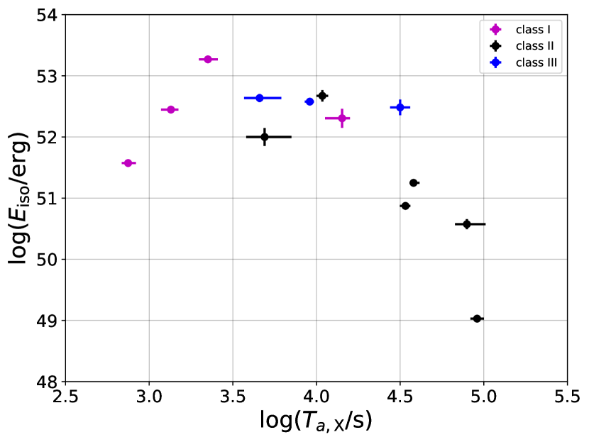
Figure 1: Total Isotropic Energy, ${E_{\rm iso}}$ as a function of the time at the end of the plateau phase, ${T_{\rm a,X}}$ in the X-ray band. Purple, black and blue points represent GRBs in the three different classes I, II, III respectively (see Supplementary Tables 1, 2, 3). The errors correspond to a significance of one sigma. Note that these three classes, selected only based on the temporal indices of their X-ray and optical afterglow light curves, are correlated with the prompt phase energy as well as the break time: each class occupies a different region in the ${E_{\rm iso}}$ – ${T_{\rm a,X}}$ parameter space. This fact provides a further, independent tool that increases our confidence in the selection criteria we use for these classes. The source data to reproduce this figure are provided as a Source Data file.

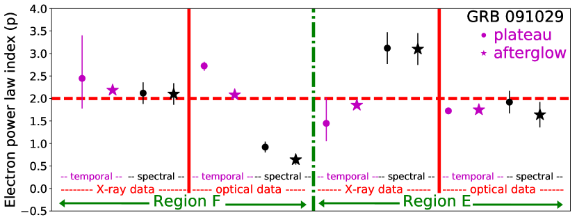
Figure 2: An example demonstrating how we determine the relevant region for a given source as well as the electron power-law index ($p$) shown in Table 1. For each burst (in the cases presented here, GRB 091029), we consider eight independent indicators, namely the temporal (purple) and spectral (black) slopes of both the X-ray and optical data during both the plateau (dot) and self-similar (star) phases. These eight independent measurements are inserted into the theoretical predictions given in Supplementary Table 5 to calculate the values of the electron power-law index, under the assumption that the data is in region F (left side) or E (right side). The obtained eight independent measurements (for each region, F and E), are then displayed side by side. The vertical green dash-dot line separates the analysis carried under the assumption that the emission is in region F (left) and E (right), the vertical red lines separates X-ray and optical data and the dashed horizontal line marks $p=2$. The errors correspond to a significance of one sigma. For X-ray data, the independent calculations converge in region F to a single value of $p\simeq 2.15$ while the assumption that the outflow is in region E leads to a diverging result. Similarly, for optical data, the assumption that the emission is in region F leads to a divergence, while the assumption that it is in region E provides a consistent value of $p\simeq 1.85$. We therefore conclude that the X-ray emission of GRB 091029 is in region F, and the optical emission is in region E. Therefore, this burst is classified as being in class I. The source data necessary to reproduce this Figure are provided as a Source Data file.

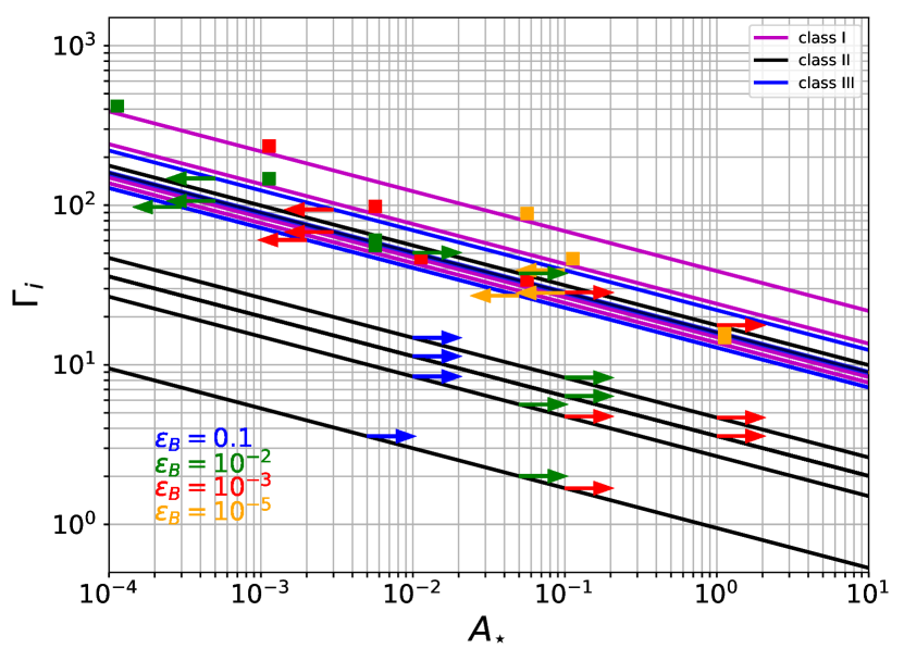
Figure 3: The initial GRB jet Lorentz factor, $\Gamma_{i}$ and the ambient density, $A_{\star}$. They are marked by lines, each corresponds to a different GRB. From top to bottom: GRBs 080607, 110213A, 060714, 080310, 061121, 060605, 130831A, 091029, 050319, 060729, 060614, 100418A, and 171205A. Purple, black and blue lines represent the GRBs in classes I, II and III respectively. For a given $A_{\star}$, we determine the value of $\Gamma_{i}$ by using Supplementary Equation (20) and knowing the burst energy and transition time $T_{\rm a,X}$. This gives the lines. In order to further constrain the values of these parameters, we assume knowledge of magnetization, $\epsilon_{B}$, and use Supplementary Equation (21) to deduce direct values of $A_{\star}$ and $\Gamma_{i}$ (squares) for class I. For classes II and III, we instead use Supplementary Equations (24) and (25) to compute the lower (upper) and upper (lower) limits of $A_{\star}$ ($\Gamma_{i}$) respectively. These limites are represented by arrows. In all classes, the constraint put by the magnetization ($\epsilon_{B}$) is inversely proportional to the ambient density. We mark on the plot the values obtained for $\epsilon_{B}=0.1,10^{-2}$, $10^{-3}$ and $10^{-5}$ which are associated to the blue, green, red and orange colors, respectively. The lowest value of Lorentz factor (4, blue arrow) is obtained for GRB 171205A. Due to its low luminosity, $L_{\rm iso}=5.6\times 10^{46}$ erg/s, the prompt emission radius is above the photospheric radius, as shown in Fig. 4. In addition, this GRB is found to exhibit a black-body emission with a low temperature in the X-ray spectra, later on this component cooling into the UV and optical range over time [68, 69]. The source data to reproduce this figure are provided as a Source Data file.

Figure 4: Ratio of the prompt emission radius, $R_{\rm E}$ and the photospheric radius, $R_{\rm ph}$ versus total isotropic energy $E_{\rm iso}$. Purple, black and blue points represent GRBs in the three different classes I, II, III respectively (see Supplementary Tables 1, 2, 3). The errors correspond to a significance of one sigma. The low luminous GRBs with lowest Lorentz factor (GRBs 060614, 060729, 100418A and 171205A) are marked by their names. For these GRBs we consider $\epsilon_{B}=0.1$, leading to typical initial jet Lorentz factor $\Gamma_{i}\approx 10$ and ratio $R_{\rm E}/R_{\rm ph}\sim 5-25$, but for GRB 100418A, which is marginally consistent with $R_{\rm E}/R_{\rm ph}\sim 1$. For all other GRBs, we assume $\epsilon_{B}=10^{-3}$ when making this plot, and a variability time $\Delta t_{\min}$ taken from Refs. [41, 42], except for GRB 060714, where $\Delta t=5$ s is assumed based on data from the Swift-BAT light-curve. We point out that a higher value of $\epsilon_{B}$ increases this ratio. The vertical green lines associated to each GRB illustrate the possible ratios of $R_{\rm E}/R_{\rm ph}$ obtained for magnetization in the range $10^{-3}\leq\epsilon_{B}\leq 0.7$. The horizontal red line indicates $R_{\rm E}/R_{\rm ph}=1$. It shows that in all cases, sufficiently high value of $\epsilon_{B}$ within the examined range leads to $R_{\rm E}>R_{\rm ph}$. The source data to reproduce this figure are provided as a Source Data file.

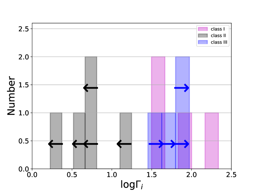
Figure 5: Histogram of the initial jet Lorentz factors for the 13 GRBs in our sample. These values are obtained by assuming that the fraction of energy in the magnetic field is $\epsilon_{B}=10^{-3}$. The purple bars represent values deduced directly from the data (class I), the black bars are upper limits (class II) and the blue bars are lower limits (class III). Upper and lower limits are also marked by arrows. The average value of the initial GRB jet Lorentz factor is $\langle\Gamma_{i}\rangle\approx 51$ (median is 32), although the range span is between $\leavevmode\nobreak\ 1.7\lesssim\Gamma_{i}\leq 218$ (see Table 3). We point out that GRB 080607 which has the highest value of $\Gamma_{i}$ has a large gap in its X-ray LC between the plateau and self-similar phases. Furthermore, GRB 171205A which has the lowest value of $\Gamma_{i}$ is associated with SN 2017iuk, therefore, both the optical plateau and self-similar slopes of this burst are effected by the SN bump (see, Supplementary Method Supplementary Method 1b. Optical data and fitting process for further discussion). The source data to reproduce this figure are provided as a Source Data file.

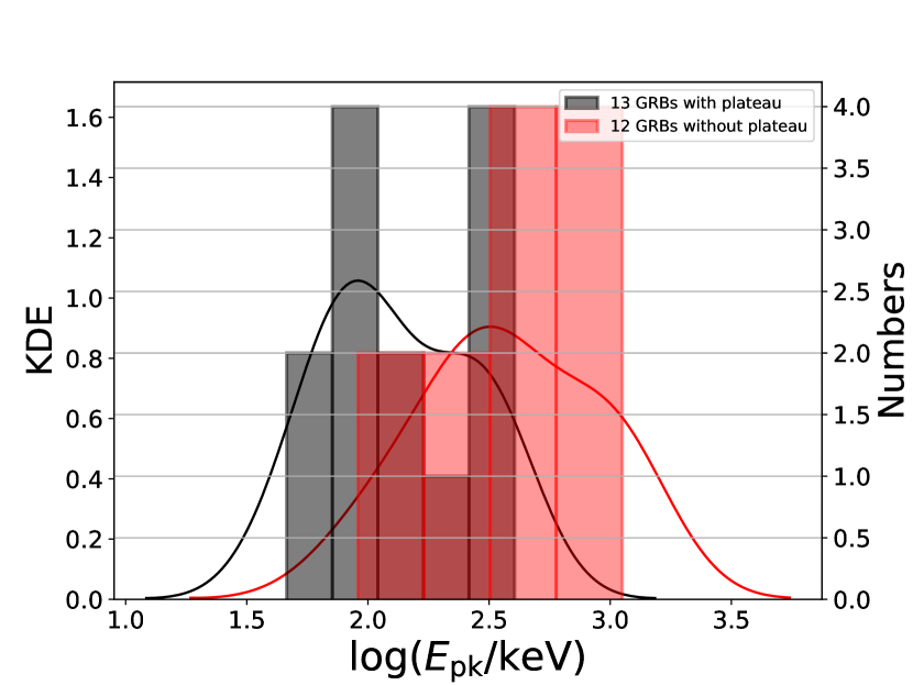
Figure 6: Distributions of peak energy, $E_{\rm pk}$. The black bars represent the 13 GRBs with plateau phases in our sample, the red bars represent 12 GRBs without plateau phases presented in Table 6 of Ref. [49]. Note that GRBs 050319, 061021 as well as early GRBs observed before the launch of Swift-BAT in Ref. [49] were discarded. In the panel the right-hand ordinate is the number of burst in each histogram bin and the left-hand ordinate is the value of the kernel density estimation (KDE), which is shown by the black and red curves for each sample respectively. Clearly, "plateau" bursts have a lower peak energy than other bursts. This result is consistent with the idea that jets in these bursts have a lower initial jet Lorentz factor. We also performed a Kolmogorov-Smirnov test (KS test: D = 0.60 and p = 0.014) which can clearly show if these two samples originate from the same population. The KS test result shows that there is only 0.14% chance for these samples to have originated from the same population and they differ with 60%. We view this as another hint towards understanding the difference between GRBs that do show a plateau and those do not. The source data to reproduce this figure are provided as a Source Data file.

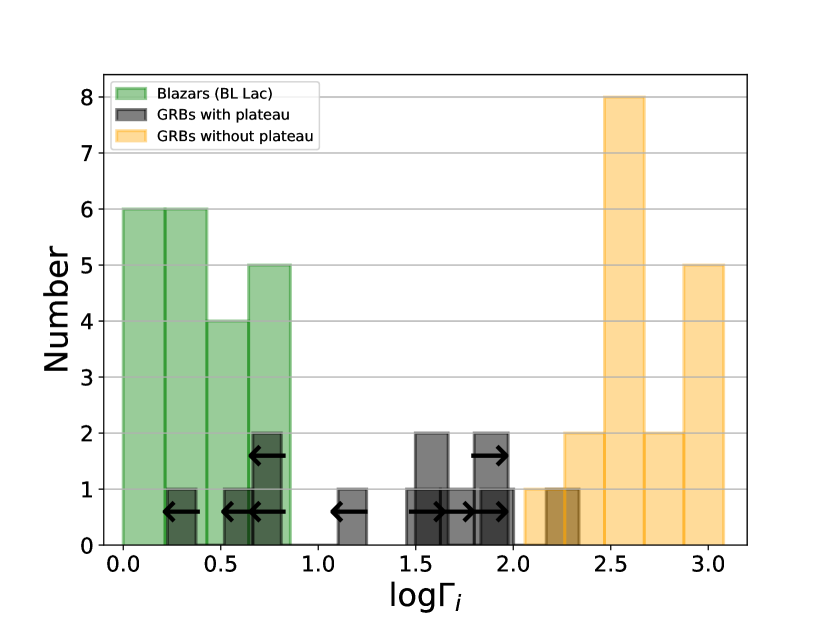
Figure 7: Histogram of the initial jet Lorentz factors. Black represents the GRBs in our sample, as they appear in Fig. 5. Yellow represents GRBs observed by the Fermi-LAT instrument, taken from Ref.[3], whose jet Lorentz factor is deduced from the opacity argument (GRBs 090926A, 090902B, 090510, 080916C; see Ref.[3], figure 11) and other GRBs that do not show a plateau phase (except GRBs 050319 and 061021), taken from Ref.[49] (table 6 therein). Green represents the inferred lower limit to the Lorentz factor of BL Lac objects (Blazars), taken from Ref.[70] (see their table 2A). The values of the Lorentz factor we found, of few tens, fills the gap that previously existed in the range of initial jet velocities. The source data to reproduce this figure are provided as a Source Data file.

Supplementary Information

Supplementary Method 1. Sample and data analysis

We use the sample of 222 GRBs with plateau phase and with known redshifts defined in Ref.[71] (see also Refs. [72, 73, 74, 75]). These GRBs were detected by the Neil Gehrels Swift Observatory [76] from January 2005 until August 2019. They represent the 56% of the GRBs (394) with known redshifts observed by the Swift satellite in this period. To define this sample, two criteria are used by Ref.[71], (1) the X-ray light curve of GRBs must have at least one data point in the beginning of the plateau phase and (2) possess a plateau angle smaller than $41^{\circ}$. The choice of the $41^{\circ}$ comes from the analysis performed in Refs. [77, 78] to allow a more reliable identification of the plateau itself. The plateau phase is identified by fitting the Swift-BAT and XRT data together with the phenomenological Willingale model [79].

In order to make our analysis as reliable as possible, we further limit the sample to burst having the best quality observations. Therefore, we added three further criteria to the ones used by Ref.[71]. We require (i) a long lasting plateau phase spanning several thousands of seconds with a temporal X-ray slope larger than $-0.7$, followed by a power-law decay phase at later times (the self-similar phase). (ii) A sufficiently large number of data points ($\gtrsim$ 5 which corresponds to the number of parameters used to fit the data with one break) during the plateau and self-similar phases to enable the fits to give well constrained parameter values. For this to be valid, we excluded all X-ray flares (see figure 1 of Ref.[80]) defined in the online Swift repository from the analyzed data. When, after removing the flares we end up having too few data points either during the plateau or the self-similar phase, we excluded the GRB from the analysis.

After applying those criteria, we ended up with 130 GRBs having a well-defined X-ray plateau emission that is followed by a power-law decay phase (which can be interpreted as the late afterglow, or the self-similar phase). Our last criteria is to require an optical counterpart at around the same time as X-ray data. We find 24 GRBs in Ref.[72] consistent with all these criteria. However, we only have full access to the published optical data. Therefore, we perform the analysis and confront our model only to a representative sample made of 13 GRBs listed in Supplementary Tables 1, 2, 3.

Supplementary Method 1a. X-ray data and fitting process

The X-ray count rate light curves (hereinafter LCs) [88] of each 13 GRBs have been downloaded from the online Swift repository , for the full Swift-XRT bandpass ($E_{\rm min},E_{\rm max}$) = (0.3,10) keV. We then fit each light-curve with a two or three-segments broken power-law (BPL) model (i.e. with one or two break times) depending on the required break during the late afterglow phase (self-similar phase). The latter break generally coincides with a jet break (see the canonical X-ray afterglow light curve in Ref.[80], figure 1 therein). The X-ray light-curve of 13 GRBs together with our fit results are presented in Supplementary Figs. 1a, 2a, 3a, 4a, 5a, 6a, 7a, 8a, 9a, 10a, 11a, 12a, 13a.

The two-segments BPL model is characterized by the following simple function

$$f(t)=A\times\left\{\begin{array}[]{ll}(t/t_{\rm b})^{-\alpha_{1}}&{\rm for}\leavevmode\nobreak\ t<t_{\rm b},\\ (t/t_{\rm b})^{-\alpha_{2}}&{\rm for}\leavevmode\nobreak\ t>t_{\rm b}\end{array}.\right.$$ (1)

In this expression t is the time, $t_{\rm b}$ is the break time, A is the amplitude at the break time, $\alpha_{1}$ and $\alpha_{2}$ are the temporal slopes before and after the break time respectively. The three-segments BPL model consider of an additional break and segment.

During the fit, we excluded the early steep decay segment and highly significant emission bumps following the GRB prompt tails (see Ref.[80] figure 1 therein) defined in the online Swift repository. In addition, we removed all flares. Some faint flares are not defined in the online Swift repository, however, they affect the definition of the break time at the end of the plateau phase ($T_{\rm a}$) in individual GRB light curves. Comparing the optical and the X-ray break times we found that the X-ray break time ($2.8\pm 0.6\times 10^{3}$ s) in the LC of GRB 091029 is earlier than the optical one ($1.54\pm 0.11\times 10^{4}$ s). This is in contrast with the theoretical expectation that, due to the rise in the cooling frequency, the transition time is expected to be earlier in the optical band than in the X-ray band. Therefore, by checking the BAT and XRT unabsorbed flux density light curves at 10 keV retrieved from the online Swift burst analyser repository, we identified a flare between $1379-2421$s in the X-ray LC of GRB 091029. Then we objectively removed this flare in the X-ray LC of this burst. It is also important to note that the flares in the online Swift repository using the phenomenological Willingale model [79] are indicative and not precise.

It is also known that the data obtained by window timing (WT) mode can be effected more from the high latitude emission than the data obtained by photon counting (PC) mode because the WT mode is usually taken at early times as it measures the flux better when the source is bright (see Ref.[89] for more explanation). Light-curves containing both WT and PC data require special attention to analyse the effect of different data type on the slopes. To avoid this issue, we only used data acquired in PC mode even if WT mode data exist (namely for GRB 061121 and GRB 060605). Once the data were retrieved and reduced, we perform a fit to determine the X-ray temporal slopes ($\alpha_{\rm p,X}$, $\alpha_{\rm A1,X}$, $\alpha_{\rm A2,X}$) and the time of the transition between the two components, ${T}_{\rm a,X}$ as well as the time of the jet break ${T}_{\rm b,X}$.

An example of the fitting process: To visualise the fitting process, we illustrate in Supplementary Fig. 3a the X-ray count light-curve obtained from GRB 060614 by the Swift-XRT instrument (over the period of PC mode data acquisition). The data are superposed with the fits results obtained for a three-segments BPL model, i.e. with two break times. To perform the fit, we used the Bayesian analysis tool emcee. We set up the computation with 64 MCMC walkers, a 100 burn-in period and the 5000 MCMC steps. We chose these steps taking into account the auto-correlation time. The value of the MCMC steps can slightly change for each GRB depending on the auto-correlation time but the choice of 5000 steps is the one that guarantees that the auto-correlation time is always taken into account. We employ the following uninformative prior distributions for the fit parameters

$$\left\{\begin{aligned} Pr(N)&=\mathcal{U}(-5,5),\\ Pr(\alpha_{\rm p})&=\mathcal{U}(-5,5),\\ Pr(\alpha_{\rm A1})&=\mathcal{U}(-5,5),\\ Pr(\alpha_{\rm A2})&=\mathcal{U}(-5,5),\\ Pr(\log(T_{\rm a}))&=\mathcal{U}(2,4.5),\\ Pr(\log(T_{\rm b}))&=\mathcal{U}(4.5,6),\\ Pr(\log(V))&=\mathcal{U}(-15,12),\end{aligned}\right.$$ (2)

where $N$ is the normalisation, $\alpha_{\rm p}$, $\alpha_{\rm A1}$ and $\alpha_{\rm A2}$ are the slopes during the plateau, in the self-similar phase and following the jet break respectively. Here, $\mathcal{U}$ notes the uniform prior. The characteristics times $T_{\rm a}$ and $T_{\rm b}$ mark the end of the plateau and the jet break respectively. Finally $V$ is a nuisance parameter measuring the spread of the data. The parameter range for the normalisation can change depending on the band (X-ray or optical) in which the fit is performed.

As a Specific example, we show the fit parameters of GRB 060614 in Supplementary Table 4. The corner plot of the posterior probability distributions of the fit parameters and the covariances between the fit parameters is displayed in Supplementary Fig. 14.

The temporal fit parameters in the X-ray band obtained for all 13 GRBs in our sample are presented in Supplementary Tables 1, 2, 3, for different classes I, II, and III respectively. The definitions of these classes are explained in Results subsection ‘Sample classification’ in the main manuscript.

The X-ray spectral slopes ($\beta_{\rm p,X}$, $\beta_{\rm A1,X}$, $\beta_{\rm A2,X}$) of twelve GRBs out of thirteen (all GRBs but GRB 060729) for the time intervals defined by the characteristic times of the X-ray light-curve are also obtained from the online Swift repository and presented in Supplementary Tables 1, 2, 3. It is important to note that the photon index (which is equal to $\beta+1$ where $\beta$ is the spectral index) is presented in the online Swift repository. For GRB 060729, we used the result from the spectral analysis of Ref.[91] since the value of the spectral index is not given by the online Swift repository. These X-ray spectral and temporal parameters together with temporal slopes obtained from the temporal fit are combined into the closure relations ($F_{\nu}\propto t^{-\alpha}\nu^{-\beta}$) as explained in the Result subsection ‘Closure relations and determination of the electron power-law indices’. This relations are presented in Supplementary Figs. 15 and 16.

Caveats for the X-ray analysis for specific GRBs:

• GRB 080607. For this burst, the error of the temporal slope during the plateau phase is large. This is due to the lack of the data points at the end of the X-ray plateau phase. The slope after the plateau phase is rather steep. However, the later (last) slope is more compatible with the expectations from the self-similar phase, see, Supplementary Fig. 8a. Therefore, we used later slope presented in Supplementary Table 1. The light-curve has two flares before the onset of the plateau phase. The transition between the peak-flux of the second flare and the plateau phase is well represented by a BPL, with steep slopes $-2.27^{+0.07}_{-0.07}$ and $-1.42^{+0.25}_{-0.30}$, separated at a break time of $341^{+31}_{-28}$s. The post-flare slopes are similar to the slopes found after the plateau phase. Therefore, either another flare might exist during the plateau or the plateau slope might be steeper with a break later than the ${T}_{\rm a,X}$ obtained here.

• GRB 130831A: The lack of data in the X-ray LC of this GRB between $10^{3}$ and $10^{4}$s, typical for the duration of the plateau, affects the measurement of ${T}_{\rm a,X}$, see Supplementary Fig. 12a. We tried to fit the light curve with a model composed of three power-law and two breaks. For this model, we found that $\log(T_{\rm a,X}/\rm s)\leavevmode\nobreak\ =\leavevmode\nobreak\ 3.08_{-0.18}^{+0.28}$. This break is consistent with being achromatic in both X-ray and optical bands (see, Supplementary Method Supplementary Method 1b. Optical data and fitting process). However, due to the large uncertainty on $T_{\rm a,X}$ we found that fitting the light curve with a single break provides a better fit. Therefore, in our analysis we used the parameters obtained for the model with one temporal break. These parameters are given in Supplementary Table 1. In addition, before the lack of data, we also define a faint flare between $595-811$ s in the X-ray LC of this burst. This flare coincides with the beginning of the optical flare, see Supplementary Fig. 12b. Therefore, we also performed a fit without this flare. We found that the both slopes ($-0.80_{-0.03}^{+0.03}$ and $-0.98_{-0.06}^{+0.06}$ respectively with a break at $1.0_{-0.16}^{+0.25}\times 10^{4}$ s) are consistent with the expected slope ($\sim-1.2$) in a self-similar phase. This result is also consistent with a previous study in Ref.[92]. We then conclude that either this GRB is not the best representation of the GRBs that show plateau phase or the lack of the data is misleading the results.

Supplementary Method 1b. Optical data and fitting process

Below, we describe the details of the fitting procedure in the optical band for each GRB in our sample. Before making the fits and if needed, the data were first transformed to the AB magnitude system. The results of the fits (in the temporal regions of interest) are presented in Supplementary Tables 1, 2 and 3. The following detailed explanations for each GRB independently are split depending on the origin of the data.

For GRB 091029, GRB 110213A, GRB 130831A and GRB 171205A, the optical data were retrieved from all possible published sources listed in Supplementary Table 1. For each of these bursts, we compiled a large set of data obtained in different bands from different instruments. The temporal fits are performed simultaneously in each band, which means that we consider all the bands at the same time, only changing the normalisation between the observation bands. Our aim here is to reduce the dependence on a single instrument and a single band in the determination of the temporal slopes and the break times. This method provides tight estimations of the fit parameters.

• GRB 091029: The photometric data set was retrieved from tables 5, 6, 7, 8, 9 of Ref.[93]. The data are displayed alongside our fit results in Supplementary Fig. 9b. We fit the data between 427.7s and $2\times 10^{5}$s with a three-segment broken power law model (i.e. with two breaks, hereinafter two-break model). Although later data exist, the flattening in the U-band likely indicates an external source of radiation, such as the contribution from the host galaxy. Therefore, data after $2\times 10^{5}$s are excluded from the fit. The first temporal break at $3.7^{+0.3}_{-0.2}\times 10^{3}$s is interpreted as the beginning of the plateau, although the earlier (i.e. before the plateau) slope is $-0.60_{-0.01}^{+0.02}$.

• GRB 110213A: The photometric observations are obtained from table 4 of Ref.[94]. They are displayed alongside our fit results in Supplementary Fig. 11b. The optical light-curve of this GRB has two peaks. The brightest peak is at 263s and the second peak is at 4827s. This flare can be clearly seen in the unabsorbed flux density light curve (see Swift-BAT-XRT at 10 keV in the online Swift burst analyser repository). This flare produces a rising slope during the X-ray plateau phase, however, it has a negligible effect on the value of break time at the end of the plateau phase $T_{\rm a,X}$.

• GRB 130831A: The photometric data of this burst is obtained from the VizieR Online Data Catalog [95]. The data are displayed alongside our fit results in Supplementary Fig. 12b. A flare can clearly be identified between 425s and 3400s, therefore, this time interval is not considered in our fit. The flare interpretation of this re-brightening is further supported by the fact that we found the temporal slopes before 425s and after 3400s to be the same. The light curves in the Rc and Ic bands flatten after $10^{5}$s, most likely due to an external source. Shortly later, this flattening also appears in all other bands. Therefore, the data after $10^{5}$s are discarded from our analysis.

• GRB 171205A: The photometric data set is obtained from Ref.[69]. The data set is displayed alongside our fit results in Supplementary Fig. 13b. Since this GRB is associated to the supernovae SN 2017iuk, the optical data start to rise at ${T_{\rm b,O}}=1.73\times 10^{5}$ s. We fit all the data before the peak of the supernovae (SN) at $9.51\times 10^{5}$ s with a two break model. The first break (${T_{\rm a,O}}$) represents the transition from the plateau to the self-similar phase, while the second break, at ${T_{\rm b,O}}$ marks the rise of the optical light curve due to the supernovae contribution. We find that the temporal slopes are somewhat shallower, and even slightly rising than in other bursts. Moreover, the break time ${T_{\rm a,O}}$ occurs earlier in the optical band than the X-ray band. We believe that this may be due to the SN bump after $\approx 2$ days [69].

For GRB 050319, GRB 060605, GRB 080607 and GRB 100418A, we used the optical data from table 8 of Ref.[91]. In that paper, all available data obtained from different instruments were collected. The details of the fitting process is given below for each of these GRB.

• GRB 050319: We use a two-break model to fit the optical light-curve until the observer time $t=5.34\times 10^{5}$ s, after which the observations show a steep flux decrease with an exponent steeper than $-1.2$ (which is theoretically expected from the self-similar phase.) The first break is observed at time $371^{+31.6}_{-28.6}$ s, which is too small to be the end of the plateau in the framework of our model. We therefore consider the break at $3.58^{+0.30}_{-0.32}\times 10^{4}$ s to be the end of the plateau. In any case, the optical slopes of each phase are not very different: the early (before the plateau) slope is $-0.41_{-0.01}^{+0.02}$, the slope of the plateau is $-0.59_{-0.01}^{+0.01}$ and the slope during the self-similar expansion is $-0.64_{-0.01}^{+0.02}$.

• GRB 060605: We fit the data between 185 s and $2\times 10^{4}$ s with with a two-break model. After the time $t=2\times 10^{4}$ s, the optical data flattens in all bands, see, Supplementary Fig. 2b. Therefore, this data is not included in the fit.

• GRB 080607: The LC of this has three breaks at around 89 s, at $793^{+77}_{-64}$ s and at $T_{\rm a,O}=2.55^{+0.26}_{-0.12}\times 10^{3}$ s, see Supplementary Fig. 8b. Since we are interested in the late time evolution, we fit the data starting at 89 s. The temporal slope before the plateau phase is $-1.22^{+0.01}_{-0.02}$, which is similar to the slope of the self-similar phase, see Supplementary Table 3. Contrary to the X-ray band (see above, Supplementary Method Supplementary Method 1a. X-ray data and fitting process), the plateau phase in the optical band is clearly identified and characterized.

• GRB 100418A: In our analysis of the optical data, we excluded the data only reported in the GCN (Gamma-ray Coordination Network). For this burst specifically, we fit a one-break model to the data.

The optical LC of the rest of the GRBs in our sample (namely GRB 060614, GRB 060714, GRB 060729, GRB 061121, and GRB 080310) are taken from Ref.[96] (see also, Ref.[97] for the details). These data were obtained by the Swift Ultraviolet/Optical (UVOT) instrument in bands V, B, U, W1, M2 and W2. In Ref.[96], all the LCs were normalized to the U band, and we use these normalised LCs in our analysis. The details of the fitting process are given below for each GRB.

• GRB 060614: We fit the data between $4.84\times 10^{3}$ and $8.39\times 10^{5}$ s. Indeed, at early times between 113.16s and 379.87s, the LC has a steep decay which coincides with the steep decay observed in X-ray data, see Supplementary Fig. 3a. This decay is therefore interpreted as the end of the prompt phase. Moreover, no observations were performed between 380s and $4.8\times 10^{3}$s. At times larger than $8.39\times 10^{5}$s the LC flattens which is interpreted as host galaxy contribution, see Supplementary Fig. 3b.

• GRB 060714: The observations of this burst are scarce with large errors. We excluded the last data point at $1.49\times 10^{7}$s from the fit since it is a clear outlier. We also did not included the non-detection limits in our analysis. With 8 data points left, a break can clearly be identified and the parameter of a one-break model be constrained, even though the observations after $10^{5}$s have large errors, see Supplementary Fig. 4b.

• GRB 060729: We fit the data between $266$s and $1.12\times 10^{6}$s. At earlier times, the optical flux rises, and at later times it flattens with a break at $\log(t)={6.16}_{-0.03}^{+0.02}$, while the slope after the break is $-0.16_{-0.07}^{+0.07}$, see Supplementary Fig. 5b.

• GRB 061121: We fit the data between $t=104.97$ and $1.66\times 10^{5}$ s. At early time between 69.19s and 89.97s, the LC has an optical flare which coincides with the X-ray flare defined in the online Swift repository. At later times, the data flattens. We further exclude the early optical bump seen between 143.45 and 568.48 s to have a better identification of the plateau slope and the break time ${T_{\rm a,O}}$, see Supplementary Fig. 6b. If our fit would include the decay of this bump (namely, starting at 230 s), its fitted slope and the break time would be $-1.01^{+0.05}_{-0.06}$ and $\log(T/\rm s)=3.12^{+0.06}_{-0.06}$ respectively. However, we would find that the later slopes ($-0.45^{+0.06}_{-0.05}$, $-0.93^{+0.07}_{-0.08}$ respectively) and the later break time ($\log(T_{a}/\rm s)=4.08^{+0.10}_{-0.10}$) would be compatible with the fit parameters presented in Supplementary Table 3. Therefore, the effect of removing the second optical bump from the analysis is negligible.

• GRB 080310: The first data point at 132.39s has a much lower flux than during the plateau. This data point can be part of the rise at early time. Such a rise is clearly seen in some of the optical LC in our sample (e.g., GRB 060605). Therefore, it is discarded from our analysis. Moreover, we also did not include in our analysis the observation with no detection, see, Supplementary Fig. 7b.

The optical spectral slopes ($\beta_{\rm p,O}$, $\beta_{\rm A1,O}$, $\beta_{\rm A2,O}$) of twelve GRBs out of thirteen in our sample (all except GRB 130831A which does not have a published one) are obtained from the literature: data of GRBs 050319, 060605, 060614, 060729, 061121, 080310, 080607 and 100418A are presented in Ref.[91]; GRB060714 in Ref.[98]; GRB091029 in Ref.[93]; GRB110213A in Ref.[94]; and GRB171205A in Ref.[69]. All these slopes are given in Supplementary Tables 1, 2, 3 for the different classes I, II, III respectively. These spectral slopes are also combined into the closure relation ($F_{\nu}\propto t^{-\alpha}\nu^{-\beta}$) in Supplementary Figs. 15 and 16 together with temporal slopes obtained from the optical temporal fit. This relation is as explained in the Result subsection ‘Closure relations and determination of the electron power-law indices’.

Supplementary Method 1c. Flux Ratio

X-ray energy flux ($\nu F_{\nu}$): The unabsorbed flux density ($F_{\nu}$) light curves of XRT at 10 keV [89] are obtained from the online Swift burst analyser repository. These flux density LCs are already corrected for absorption from both the galactic and host galaxy. In our analysis, we convert these light curves from flux density (Jy) to energy flux (${\rm erg\leavevmode\nobreak\ cm^{-2}\leavevmode\nobreak\ s^{-1}}$) at 10 keV ($\nu$ = $2.42\times 10^{18}$  Hz). Then, we used these energy flux LCs to compute the $\nu F_{\nu}$ X-ray flux at the end of the plateau phase at ${T_{a,\rm X}}$ and at another specific time, typically, $1000$s.

Optical energy flux ($\nu F_{\nu}$): For computing the energy flux in the optical band, all the LCs are corrected for both the galactic and the host galaxy extinctions. i) The galactic extinction along the line of sight is obtained from the IRSA webpage for the U band filter. It is computed with the method introduced in Ref.[99]. ii) The extragalactic reddening E(B - V) of all GRBs (except GRBs 060714 and 100418A) are obtained during the plateau phase and the references are listed in Supplementary Table 6. We first used these values to compute the host galaxy extinctions in the V-band (except for 060714 for which we used the value provided in Ref.[100]). The host galaxy extinction $A_{v,\rm host}=R_{v}\times E(B-V)$ is computed by using one of the three visual extinction to reddening ratio, $R_{v}$, of 3.08, 3.16, 2.93 for the Milky Way, Large and Small Magellanic Clouds (MW, LMC and SMC) extinction laws[101] respectively. The type of extinction law is defined in the reference papers and they are also given in Supplementary Table 6. Second, we use these extinctions together with $A_{\rm u,host}=1.666\times A_{\rm v,host}$ see, details in Ref.[101], to compute the host galaxy extinction in the U band. Both extinctions (galactic and host galaxy) for each GRBs are given in Supplementary Table 6. Note that the flux density of four GRBs (namely GRB 050319, GRB 060605, GRB 080607, GRB 100418A) taken from Ref.[91] are already corrected for both galactic and host extinction.

In details, we proceed as follows:

• For six GRBs, namely GRB 060614, GRB 060714, GRB 060729, GRB 061121, GRB 080310 and GRB 091029, the optical count rate LCs from Ref.[96] are used to compute the U-band energy flux LCs. For the conversion, we used the U-band count rate to flux conversion factor ($1.628\times 10^{-16}\leavevmode\nobreak\ {\rm erg\leavevmode\nobreak\ cm^{-2}\leavevmode\nobreak\ Angstrom^{-1}\leavevmode\nobreak\ counts^{-1}}$), as provided in the UVOT calibration website. Then, we computed the energy flux ($\nu F_{\nu}$) LCs, where $\nu$ is taken at the U-band central frequency equal to $8.65\times 10^{14}$ Hz. These U-band energy flux LCs are used to compute the $\nu F_{\nu}({\rm U})$ optical flux at a specific time namely $\sim 1000$s hereinafter dubbed reference time in the U-band $T_{\rm ref.,\rm U}$ and at the end of the plateau phase at ${T_{\rm a,X}}$.

For all other GRBs, we followed a different procedure presented below:

1. For the GRBs in Ref.[91], namely GRB 050319, GRB 060605, GRB 080707, and GRB 100418), the $\nu F_{\nu}$ optical flux at the end of the X-ray plateau phase ($T_{\rm a,X}$) are retrieved from the flux density LC in table 7 of the online material in Ref.[91]. In these cases, the frequency $\nu$ is different for each GRBs (V band $\nu=5.48\times 10^{14}$ Hz, CR and RC bands $\nu=4.55\times 10^{14}$ Hz, white band $\nu=7.79\times 10^{14}$ Hz, see Supplementary Table 6). For consistency, whenever possible we used the U-band in calculating the LC. When the U-band data was not available, we used other bands. In such case, we note that, the differences between different optical bands ($\sim 10^{15}$ Hz) are small.

2. For all other, namely GRB 110213A, GRB 130831A, and GRB 171205A, we followed the same procedure as in appendix A of Ref.[91] to convert the optical data from the AB magnitude system to the optical energy flux. Therefore, the final conversion formula is $f_{\nu}=10^{-0.4(m_{AB}+48.585)}$ where $f_{\nu}$ is the flux density in frequency, $m_{AB}$ is magnitude in AB system.

Energy flux ratio: The specific energy fluxes $\nu F_{\nu}({\rm X})$ at ${T_{\rm a,X}}$ in the X-ray band and $\nu F_{\nu}({\rm U})$ at $T_{\rm ref.,U}$ in the optical band are used to compute the energy flux ratio between the X-ray and the optical bands. The ratio is computed by [$1/(\nu F_{\nu}(\rm U)/\nu F_{\nu}(\rm X))$] and is given in the last column of Table 3 in the main text.

Isotropic energy: The Swift-BAT observations are carried in a relatively narrow energy range (15–150 keV) which prevents from measuring the peak energy. To obtain a lower limit on the isotropic energy ${E_{\rm iso}}$, we followed the same method presented in Ref.[102]. In this method, a simple power-law spectral model is adopted, i.e. $\phi(E)\propto E^{\alpha_{\gamma}}$, where $\phi(E)$ is the source photon spectrum and $\alpha_{\gamma}$ is the photon spectral index The estimate on the isotropic energy in the BAT band $E_{\rm iso}$ is then computed as

$$\centering E_{\rm iso}=\frac{4\pi{d_{\rm L}^{2}S}}{(1+{z})^{3-{\alpha_{\gamma}}}}.\@add@centering$$ (3)

where $S$ is the BAT fluence between 15 and 150 keV. Both $S$ and $\alpha_{\gamma}$ are taken from the Swift GRB table, ${d_{\rm L}(z)}$ is the luminosity distance calculated assuming a flat $\Lambda$CDM cosmological model with cosmological parameters $\Omega_{m}=0.286$ and ${H_{\rm 0}}=70\leavevmode\nobreak\ {\rm km\leavevmode\nobreak\ s^{-1}\leavevmode\nobreak\ Mpc^{-1}}$, and $z$ is the redshift.

The various parameters relevant to our study are listed in Table 2 (in main text): (i) the GRB name, (ii) its redshift ($z$), (iii) the luminosity distance (${d_{L}}$), (iv) fluence ($S$), (v) photon spectral index ($\alpha_{\gamma}$), (vi) isotropic energy (${E_{\rm iso}}$) in the Swift-BAT band, (vii) burst duration $T_{90}$ which is obtained from the Swift GRB table, (viii) the time at the end of the X-ray plateau phase ($T_{\rm a,X}$), (ix) $\nu F_{\nu}$ X-ray flux and (xi) $\nu F_{\nu}$ optical (U band) flux at $T_{\rm a,X}$, (x) a reference time in the optical band called $T_{\rm ref.,U}$ (typically at around 1000 s), (xii) $\nu F_{\nu}$ X-ray flux and (xiii) $\nu F_{\nu}$ optical (U band) flux at the reference time $T_{\rm ref.,U}$. The isotropic energy ($E_{\rm iso}$) and a time at the end of the X-ray plateau phase (${T_{\rm a,X}}$), firstly discovered by Ref. [103, 104, 105], are presented in Fig. 1 (main text).

Supplementary Method 2. Theoretical model

The key to understanding the observed signal within the framework of our model is the realization that the end of the plateau corresponds to the transition from a coasting phase to a self-similar (decaying) expansion phase of the expanding plasma. The observed signal originates entirely from ambient electrons collected and heated by the forward shock wave, propagating at relativistic speeds inside a "wind" (decaying density) ambient medium. During the transition from the coasting to the self-similar phases a reverse shock crosses the expanding plasma. However, the contribution from electrons heated by the reverse shock is suppressed due to (i) the declining ambient density which implies that the ratio of plasma density to ambient density remains constant (in a conical expansion), and (ii) its slower speed, which translates into less energetic electrons that emit at much lower frequencies than forward shock heated electrons, implying that the contribution to the optical and X-ray bands is negligible.

To understand how this transition affects the observed spectra, we first describe the radiative mechanism adopted, which is the classical synchrotron emission from a power-law distribution of electrons, injected into the radiation zone with a power-law index $p$, namely $N_{el}(\gamma)d\gamma\propto\gamma^{-p}$ above a minimum value $\gamma_{m}$. Both theory [106] and observations [107] suggest a typical value of $p$ such that $2.0\leq p\lesssim 2.4$. Below the injection Lorentz factor $\gamma_{m}$, it is safe to assume that the electrons have a Maxwellian (or quasi-Maxwellian) energy distribution [9, 34]. This particle distribution leads to a broken power-law spectrum, whose shape, in the relevant observed bands (frequency $\nu$), depends on whether the peak frequency, $\nu_{m}$ (defined in Supplementary Equation (6)) is above or below the cooling frequency, $\nu_{c}$ (defined in Supplementary Equation (7)). At low frequencies, one needs to consider the self-absorption process, whose contribution is neglected here since it is observed at frequencies lower than the optical frequency.

For $\nu_{m}>\nu_{c}$ (the so-called "fast cooling" regime, expected at early times), the possibilities (marked A–C) are

$$F_{\nu}=F_{\nu_{\max}}\times\left\{\begin{array}[]{ll}\nu_{c}^{-1/3}\nu^{1/3}&\nu<\nu_{c}<\nu_{m}\leavevmode\nobreak\ \leavevmode\nobreak\ \leavevmode\nobreak\ A\\ \nu_{c}^{1/2}\nu^{-1/2}&\nu_{c}<\nu<\nu_{m}\leavevmode\nobreak\ \leavevmode\nobreak\ \leavevmode\nobreak\ B\\ \nu_{m}^{(p-1)/2}\nu_{c}^{1/2}\nu^{-p/2}&\nu_{c}<\nu_{m}<\nu\leavevmode\nobreak\ \leavevmode\nobreak\ \leavevmode\nobreak\ C\end{array}\right.$$ (4)

At later times, $\nu_{m}<\nu_{c}$ and the plasma enters the "slow cooling" regime, in which (regions D–F)

$$F_{\nu}=F_{\nu_{\max}}\times\left\{\begin{array}[]{ll}\nu_{m}^{-1/3}\nu^{1/3}&\nu<\nu_{m}<\nu_{c}\leavevmode\nobreak\ \leavevmode\nobreak\ \leavevmode\nobreak\ D\\ \nu_{m}^{(p-1)/2}\nu^{-(p-1)/2}&\nu_{m}<\nu<\nu_{c}\leavevmode\nobreak\ \leavevmode\nobreak\ \leavevmode\nobreak\ E\\ \nu_{m}^{(p-1)/2}\nu_{c}^{1/2}\nu^{-p/2}&\nu_{m}<\nu_{c}<\nu\leavevmode\nobreak\ \leavevmode\nobreak\ \leavevmode\nobreak\ F\end{array}\right.$$ (5)

Here, $\nu_{m}$ is the typical emission frequency from electrons at the peak of the distribution, namely having Lorentz factor $\gamma_{m}$, and is given by (for an on-axis observer)

$$\nu_{m}^{ob}=\frac{3}{4\pi}\frac{qB}{m_{e}c}\gamma_{m}^{2}{\Gamma\over(1+z)}=4.196\times 10^{6}B\gamma_{m}^{2}{\Gamma\over(1+z)}\rm{\,Hz},$$ (6)

where $q$ is the electron’s charge, $m_{e}$ is the electron’s mass, $c$ is the speed of light, $B$ is the magnetic field, $\Gamma$ is the bulk motion Lorentz factor and $z$ is the redshift. The cooling frequency $\nu_{c}$ is the frequency of emission from electrons whose radiative cooling time is equal to the dynamical time,

$$\nu_{c}^{ob}={3\over 4\pi}{q\over m_{e}c}\left({6\pi m_{e}c^{2}\over\sigma_{T}}\right)^{2}{\Gamma^{3}\over B^{3}r^{2}(1+z)}=2.26\times 10^{45}{\Gamma^{3}\over B^{3}r^{2}(1+z)}\rm{\,Hz}.$$ (7)

Here, $\sigma_{T}$ is Thomson’s cross section, and $r$ is the plasma radius, which is related to the dynamical time (in the comoving frame) by $r\sim\Gamma ct_{\rm dyn}$. The peak flux is estimated by $F_{\nu,peak}^{ob}={1\over 4\pi d_{L}^{2}}N_{e}P_{\nu,\max}^{ob}$, where $d_{L}$ is the luminosity distance, $N_{e}$ is the number of radiating particles and $P_{\nu,\max}^{ob}=P_{tot}^{ob}/\nu_{peak}^{ob}$, where $P_{tot}^{ob}$ is the total power radiated by synchrotron emission by a single electron at $\gamma_{m}$, and $\nu_{peak}^{ob}=\nu_{m}^{ob}$. This gives

$$P_{\nu,max}^{ob}={P_{tot}^{ob}\over\nu_{m}^{ob}}={{4\over 3}c\sigma_{T}\gamma_{m}^{2}{B^{2}\over 8\pi}\Gamma^{2}\over{3\over 4\pi}{qB\over m_{e}c}\gamma_{m}^{2}{\Gamma\over(1+z)}}={2\over 9}{m_{e}c^{2}\sigma_{T}\over q}B\Gamma(1+z)=2.53\times 10^{-22}B\Gamma(1+z)\leavevmode\nobreak\ \leavevmode\nobreak\ {\rm erg\leavevmode\nobreak\ s^{-1}\leavevmode\nobreak\ Hz^{-1}}$$ (8)

We assume that all the ambient particles collected by the forward shock wave radiate. By assumption, the mass density is given by $\rho(r)=A/r^{2}$, implying that

$$N_{e}(r)={4\pi\over m_{p}}\int_{0}^{r}\rho(r^{\prime})r^{\prime 2}dr^{\prime}={4\pi Ar\over m_{p}}$$ (9)

The proportionality constant $A$ is calculated assuming that prior to its final explosion, the progenitor star ejects mass at a constant rate and at a constant velocity, resulting in $\rho(r)=n(r)m_{p}={\dot{M}\over 4\pi v_{w}r^{2}}\equiv Ar^{-2}.$ For a Wolf-Rayet progenitor, the typical values are [108], $\dot{M}=10^{-5}\,M_{\odot}\,{\rm yr}^{-1}$, and wind velocity $v_{w}=10^{8}\,{\rm cm\,s^{-1}}$. These values lead to $A=5\times 10^{11}A_{\star}\,{\rm gr\leavevmode\nobreak\ cm^{-1}}$.

Supplementary Method 2a. Dynamics, magnetic field and electron’s energy

Following an initial acceleration phase, the plasma coasts at a nearly steady Lorentz factor $\Gamma_{i}$. Once it collects sufficient material from the ambient medium, $m_{ISM}\gtrsim m_{i}/\Gamma_{i}$ where $m_{i}$ is the initial ejected mass, the flow becomes similar, and its evolution is described by the well-known self-similar solution [109]. For an instantaneous explosion releasing energy $E$ that occurs into a density gradient this solution reads

$$\Gamma(E;r)=\left({9E\over 16\pi\rho(r)c^{2}r^{3}}\right)^{1/2}=\left({9E\over 16\pi Ac^{2}r}\right)^{1/2}.$$ (10)

The relation between the Lorentz factor, radius and observed time in this case was calculated by Ref.[110], $t^{\rm ob}\simeq(1+z)r/(2\Gamma^{2}(r)c)$, enabling to express the Lorentz factor as a function of the observed time during this phase,

$$\Gamma(E,A;t^{\rm obs.})=\left({9E(1+z)\over 32\pi Ac^{3}t^{\rm ob}}\right)^{1/4}.$$ (11)

Transition from the initial (coasting) to the later (self-similar expansion) phases occurs once $\Gamma(E,A;t^{\rm ob})<\Gamma_{i}$. Thus,

$$T_{a}=(1+z){9E\over 32\pi Ac^{3}\Gamma_{i}^{4}}.$$ (12)

It is explicitly assumed that both the generation of magnetic field and acceleration of particles to high energies occur at the shock wave. The energy density behind the shock is given by the shock jump conditions, $u\simeq 4\Gamma^{2}nm_{p}c^{2}$ where $m_{p}$ is the proton mass and $n$ is the particle number density in the surrounding medium. Therefore, during the initial (coasting) phase where $\Gamma=\Gamma_{i}$, this energy density is $u(t^{\rm obs.})_{\rm coasting}=(1+z)^{2}{A/(\Gamma_{i}^{2}t_{\rm obs.}^{2})}$. We adopt the standard assumption that a fraction $\epsilon_{B}$ of this energy is used in generating a magnetic field, and a fraction $\epsilon_{e}$ is used in heating (accelerating) the electrons. During the initial (coasting) phase, this gives a magnetic field strength $B_{\rm initial}=(8\pi\epsilon_{B}u)^{1/2}=12\leavevmode\nobreak\ (1+z)\leavevmode\nobreak\ A_{\star}^{1/2}\Gamma_{i,1.5}^{-1}{t^{\rm obs.}_{3}}^{-1}\leavevmode\nobreak\ \epsilon_{B,-2}^{1/2}\leavevmode\nobreak\$G and typical electron Lorentz factor, $\gamma_{m,\rm initial}=\epsilon_{e}\Gamma_{i}\left({m_{p}/m_{e}}\right)=5.5\times 10^{3}\leavevmode\nobreak\ \Gamma_{i,1.5}\epsilon_{e,-1}$. Here and below $Q_{,x}=Q/10^{x}$.

During the deceleration phase, a similar calculation with the use of Supplementary Equation (10) gives

$$B_{late}=\left({2048\pi^{3}A^{3}c^{3}(1+z)^{3}\epsilon_{B}^{2}\over 9E{t^{\rm ob}}^{3}}\right)^{1/4}=0.74\leavevmode\nobreak\ \left({1+z\over 2}\right)^{3/4}E_{53}^{-1/4}A_{\star}^{3/4}{t^{\rm ob}_{\rm day}}^{-3/4}\epsilon_{B,-2}^{1/2}\leavevmode\nobreak\ {\rm G},$$ (13)

and

$$\gamma_{m,late}=\epsilon_{e}\Gamma{m_{p}\over m_{e}}=\epsilon_{e}\left({m_{p}\over m_{e}}\right)\left({9E(1+z)\over 32\pi Ac^{3}t^{\rm ob}}\right)^{1/4}=2040\,\left({1+z\over 2}\right)^{1/4}E_{53}^{1/4}A_{\star}^{-1/4}{t^{\rm ob}_{\rm day}}^{-1/4}\leavevmode\nobreak\ \epsilon_{e,-1}.$$ (14)

Supplementary Method 2b. Temporal and spectral signal

Using these results in Supplementary Equations (6), (7) and (8) gives the parametric dependence of the key observed frequencies and flux:

$$\nu_{m}^{\rm obs.}=\left\{\begin{array}[]{ll}4.6\times 10^{16}\leavevmode\nobreak\ A_{\star}^{1/2}\Gamma_{i,1.5}^{2}{t^{\rm obs.}_{3}}^{-1}\leavevmode\nobreak\ \epsilon_{e,-1}^{2}\leavevmode\nobreak\ \epsilon_{B,-2}^{1/2}\leavevmode\nobreak\ {\rm Hz}&{\rm(coasting)},\\ 7.2\times 10^{13}\,\left({1+z\over 2}\right)^{1/2}E_{53}^{1/2}{t^{\rm ob}_{\rm day}}^{-3/2}\epsilon_{e,-1}^{2}\epsilon_{B,-2}^{1/2}\rm{\,Hz}&{\rm(decay)},\end{array}\right.$$ (15)

$$\nu_{c}^{\rm obs.}=\left\{\begin{array}[]{ll}3\times 10^{12}\left({1+z\over 2}\right)^{-2}\leavevmode\nobreak\ A_{\star}^{-3/2}\Gamma_{i,1.5}^{2}{t^{\rm obs.}_{3}}\leavevmode\nobreak\ \epsilon_{B,-2}^{-3/2}\leavevmode\nobreak\ {\rm Hz}&{\rm(coasting)},\\ 3.7\times 10^{13}\,\left({1+z\over 2}\right)^{-3/2}E_{53}^{1/2}{t^{\rm ob}_{\rm day}}^{1/2}\epsilon_{B,-2}^{-3/2}A_{\star}^{-2}\rm{\,Hz}&{\rm(decay)},\end{array}\right.$$ (16)

and

$$F_{\nu,peak}^{\rm obs.}=\left\{\begin{array}[]{ll}6.1\times 10^{-24}\left({1+z\over 2}\right)d_{L,28.3}^{-2}\leavevmode\nobreak\ A_{\star}^{3/2}\Gamma_{i,1.5}^{2}\epsilon_{B,-2}^{1/2}\leavevmode\nobreak\ {\rm erg\leavevmode\nobreak\ cm^{-2}\leavevmode\nobreak\ s^{-1}\leavevmode\nobreak\ Hz^{-1}}&{\rm(coasting)},\\ 9.9\times 10^{-25}\,\left({1+z\over 2}\right)^{3/2}d_{L,28.3}^{-2}E_{53}^{1/2}A_{\star}\epsilon_{B,-2}^{1/2}{t^{\rm ob}_{\rm day}}^{-1/2}\,{\rm erg\leavevmode\nobreak\ cm^{-2}\leavevmode\nobreak\ s^{-1}\leavevmode\nobreak\ Hz^{-1}}&{\rm(decay)}.\end{array}\right.$$ (17)

The results of Supplementary Equations (15) and (16) imply that both at early (coasting) and later (self-similar decay) phases, the peak frequency decreases with observed time, while the cooling frequency increases with time. This have two important consequences on the spectral and temporal evolution of the observed signal: (i) At high enough frequencies, the transition always occurs from region F ($\nu_{c}<\nu$) to region E ($\nu<\nu_{c}$); and (ii) the transition always occurs at lower frequencies first- it will occur in the optical band before the X-ray band, regardless of whether the flow is in the coasting or in the decaying phase.

Using these results in Supplementary Equations (4) and (5) give the temporal and spectral dependence in each of the 6 possible regimes considered, both during the coasting and during the self-similar decay phases (see for consistency with Ref. [111]). These are summarized in Supplementary Table 5 and Supplementary Fig. 17.

These results can now be used to explain the observed signal, which is in an excellent agreement with the theoretical model. Provided that the transition to region E occurs after the end of the coasting phase, the light curve during the coasting phase is $\approx$ flat, $F_{\nu}\propto t_{\rm obs.}^{(2-p)/2}\sim t_{\rm obs.}^{0.0..-0.2}$, which is similar to the observed signal in the X-ray band in classes I and II. Since the transition to region E occurs earlier at longer wavelength, in some of the bursts in class I the optical band is already in region E, in which case a decay in the optical light curve, $F_{\nu}\propto t_{\rm obs.}^{(1-p)/2}\sim t_{\rm obs.}^{-0.5..-0.7}$ is expected. The only other option is that the transition to region E occurs at earlier times, in which case both the X-ray and the optical light curves show a decay, which is the relevant scenario for class III here.

Once the flow shifts to the self-similar decay phase, both the X-ray and the optical light curves decay as $F_{\nu}\propto t_{\rm obs.}^{(2-3p)/4}\sim t_{\rm obs.}^{-1.0..-1.3}$ if in region F, or alternatively $F_{\nu}\propto t_{\rm obs.}^{(1-3p)/4}\sim t_{\rm obs.}^{-1.25..-1.55}$ if in region E. However, the difference in the temporal index in between these two cases is only 1/4, and may not be easily identified due to the noise.

Supplementary Method 2c. Determining the physical properties of the outflow

A flat X-ray plateau indicates that the flux in the X-ray band is in region F. Assuming, for simplicity a power-law index $p=2$, Supplementary Equation (5) gives

$$\nu F_{\nu}({\rm X})^{\rm obs.}=F_{\nu,\rm peak}^{\rm obs.}\nu_{c}^{1/2}\nu_{m}^{1/2}={1\over d_{L}^{2}}c^{3}A\Gamma_{i}^{4}\epsilon_{e}$$ (18)

where we made use of Supplementary Equations (15), (16) and (17). Combining this result with Supplementary Equation (12), one finds that for bursts with known redshift, the transition time and X-ray flux provide a direct measurement of $\epsilon_{e}$:

$$\epsilon_{e}={d_{L}^{2}\over(1+z)}{32\pi T_{a}\over 9E}\nu F_{\nu}({\rm X})^{\rm obs.}$$ (19)

Furthermore, the transition time provides a strong constraint on the ambient medium and the initial Lorentz factor. This is done by writing Supplementary Equation (12)

$$A\Gamma_{i}^{4}=(1+z){9E\over 32\pi c^{3}T_{a}},$$ (20)

which is a very robust result.

A further constrain can be put by using the temporal behaviour of the optical data. In class I, the optical light curve decays, namely the optical band is in region E, and $\nu F_{\nu}(\rm U)^{\rm obs.}=F_{\nu,\rm peak}^{\rm obs.}\nu_{m}^{1/2}\nu_{\rm U}^{1/2}$ (for $p=2$). Using Supplementary Equations (15), (17), (19) and using an observed optical band $\nu_{\rm U}=8.65\times 10^{14}$ Hz as well as fiducial values for $z=1$, $E=3.16\times 10^{52}\rm erg$, $\nu F_{\nu}({\rm X})^{\rm obs.}=\rm 3.16\times 10^{-12}\leavevmode\nobreak\ erg\leavevmode\nobreak\ cm^{-2}\leavevmode\nobreak\ s^{-1}$ at $T_{a}=3000\leavevmode\nobreak\ \rm s$ and $\nu F_{\nu}(U)^{\rm obs.}=\rm 10^{-12}\leavevmode\nobreak\ erg\leavevmode\nobreak\ cm^{-2}\leavevmode\nobreak\ s^{-1}$ at 1000 s, one finds

$$A_{\star}^{7/4}\Gamma_{i,1.5}^{3}\epsilon_{B,-2}^{3/4}=4\times 10^{-3}.$$ (21)

Thus, for a given density parameter ($A_{\star}$), there is a corresponding magnetic parameter ($\epsilon_{B}$). One may therefore use an external knowledge of $\epsilon_{B}$ (e.g., an absolute upper limit of $\epsilon_{B}=1$) to completely determine the values of $A_{\star}$ and therefore of $\Gamma_{i}$. We further note that in this case, the ratio of fluxes,

$$R_{I}\equiv{\nu F_{\nu}({\rm X})\over\nu F_{\nu}({\rm U})}=\left({\nu_{c}\over\nu_{\rm U}}\right)^{1/2}\left({\nu_{\rm X}\over\nu_{\rm U}}\right)^{(2-p)/2}$$ (22)

is expected in the range $10\leq R\leq 300$ for power law indices in the range $1.8\leq p\leq 2.4$.

In class II, the optical light curve is flat, namely it is in region F. Supplementary Equations (19) and (20) are valid, and thus a direct measurement of $\epsilon_{e}$ and of $A\Gamma_{i}^{4}$ exist. However, as $\nu_{c}<\nu_{\rm U}$, the ratio of the optical and X-ray fluxes is constant,

$$R_{II}\equiv{\nu F_{\nu}({\rm X})\over\nu F_{\nu}({\rm U})}=\left({\nu_{\rm X}\over\nu_{\rm U}}\right)^{(2-p)/2}\approx 1$$ (23)

Instead, we use the fact that $\nu_{c}$ increases with time (Supplementary Equation (16)) to argue that in this case at the transition time (Supplementary Equation (12)), $\nu>\nu_{c}$. This gives a lower limit on the magnetization,

$$\epsilon_{B,-2}^{3/2}>3.1\times 10^{-3}\left({1+z\over 2}\right)^{-1}E_{52.5}A_{\star}^{-5/2}\Gamma_{i,1.5}^{-2}.$$ (24)

Thus, in this case, for a given $A_{\star}$ there is a minimum value of the magnetic field, which is inversely proportional to $A_{\star}$. Thus, again, one may use an external constraint (such as $\epsilon_{B}<1$) to constrain a minimum value of $A_{\star}$ which translates to a maximum value of $\Gamma_{i}$.

Finally, in class III both the X-ray and the optical light curves decay, namely both are in region E. In this case, Supplementary Equation (20) is valid, but not Supplementary Equation (19). It is therefore not possible to obtain a direct measure of $\epsilon_{e}$ in this case. The best constraint can be put by using the requirement that at the beginning of the plateau, at $\sim 100$ s, the X-ray frequency is already below the cooling frequency, $\nu_{\rm X}<\nu_{c}$. This translates into an upper limit,

$$\left({1+z\over 2}\right)A_{\star}^{3/2}\Gamma_{i,1.5}^{-2}\epsilon_{B,-2}^{3/2}<2.5\times 10^{-6}$$ (25)

This provides an upper limit on the value of $\epsilon_{B}$ for a given $A_{\star}$, which increases as $A_{\star}$ decrease. Using external constraint, e.g., $\epsilon_{B}=0.01$ is therefore useful in providing an upper limit on $A_{\star}$, and a lower limit on $\Gamma_{i}$. Combined with a measurement of the optical flux, this also gives a lower limit on the value of $\epsilon_{e}$.

The ratio of the X-ray to optical fluxes in this case is intermediate,

$$R_{III}\equiv{\nu F_{\nu}({\rm X})\over\nu F_{\nu}({\rm U})}=\left({\nu_{\rm X}\over\nu_{\rm U}}\right)^{(3-p)/2}\approx 10...150$$ (26)

depending on the value of $p$.

Supplementary Discussion: Comparison with other models aimed at explaining the X-ray plateau

As discussed in the main text, a plethora of models were proposed in the literature in attempts to explain the X-ray plateau. Here we discuss some of the most recent works, focusing on three topics: energy injection, reverse shock, and viewing angle.

Metzger et al. (2011) propose a millisecond protomagnetar model for GRBs [112]. In this magnetar model, the energy released by dipole radiation is predicted to be transferred to the surroundings via a magnetar wind. This wind is heated by neutrinos just after the launch of the supernova shock from a core collapse of a massive star. The outflow is collimated into a bipolar jet by its interaction with the progenitor star. As the magnetar cools, the wind becomes ultrarelativistic and Poynting flux dominated on a time-scale comparable to that required for the jet to clear a cavity through the star. Therefore, in this model the magnetic dissipation and shocks explain the prompt emission and the steep decay phase that follows. The late time flares and the X-ray plateau are thought to be powered by continuous dissipation of magnetic energy or by extraction of the residual rotational energy. Indeed, assuming a magnetic field and a spin period typical of a fast rotating neutron star, Rowlinson et al. (2014) [113] explain the correlation between luminosity and duration of the plateau phase within the $1\sigma$ uncertainties [78] in the framework of this model. A later paper by Rea et al. (2015) [114] shows that the magnetar model can be reconciled within the GRB emission of the plateau only if supermagnetars with high magnetic field strength are allowed.

In a successive paper of Stratta et al. (2018) [115] for the first time a non-ideal modelling of spindown magnetar is fitted to the afterglow data for samples of 40 long and 13 short GRBs with a well-defined plateau. The conclusion reached in that paper is that the data of both short and long GRBs can be explained within the magnetar model. However, the difference between the short and long bursts is that the long GRBs are characterized by a lower magnetic field and longer spin period compared to the short GRBs. The correlation between magnetic field and spin period follows the established physics of the spin-up line for accreting neutron star (NS) in galactic binary systems. The $B-P$ relation obtained with this sample of 53 GRBs matches spin-up line predictions for the magnetar model with mass accretion rates expected in the GRB prompt phase. The latter are $\sim$ $11-14$ orders of magnitude higher than those inferred for the galactic accreting NSs.

Matsumoto et al. 2020 [116] show a link between extended emission seen in some short GRBs and the plateau phase. They assume a continuous energy injection from a central compact object, such as a magnetar, for the origin of both emission phases. Such an extended emission lasting up to $10^{2}-10^{3}$ s is also reported in several long GRBs [117, 118]. In our study, when analyzing the full sample of 222 GRBs with known redshift and a plateau phase, we found that when such an extended emission exists, it affects the slopes of both the plateau and the following self-similar phases. The slopes for those bursts that show extended emission are steeper in both the plateau and self similar phases ($<-0.7$ and $<-1.2$ respectively) than the limit we take as an indication for a plateau (temporal slope of $>-0.7$). These are therefore excluded from our final sample.

Zhao et al. 2020 [119] argued that in a few cases, there is a steep decay following the plateau phase, after which a second plateau may exist. They interpreted this as an outcome of a central engine consisting of a rapidly spinning magnetar that collapses to a newborn black hole. When analyzing the 3 GRBs in their sample, we found that the evidence for a steep decay is not strong: the X-ray LC of these 3 bursts either contain flares, or very few data points exist.

In contrast to previous works, Çıkıntoğlu et al. (2020) [120] argue that a clear plateau phase may not be realized if the magnetic field of the nascent magnetar is in a transient rapid decay stage. Due to this stage, the spin-down power may decline too fast and cause a lack of the plateau phase. With this idea, they analyze the X-ray light curve of 6 GRBs without plateau and conclude that these GRBs might be hosting millisecond magnetars.

A different type of model was proposed by Lyutikov et al. (2017) [121] and Barkov et al. (2021) [122], in which the plateau phase, flares and possible steep slopes immediately after the plateau phase, are all explained by a dominant reverse shock. This reverse shock is different than the "classical" reverse shock predicted as part of the "fireball" model [19, 123] because it is assumed to propagate through ultrarelativistic, highly magnetized pulsar-like winds produced by long-lasting central engines. While this is an interesting idea, similar to the models discussed above, only very few GRBs observed until now seem to fit the predictions of this model. Moreover, those GRBs have several flares during their X-ray data which makes it difficult to draw a firm conclusion. Within the realm of the classical "fireball" model, contribution from the reverse shock is expected during the transition from the coasting to the similar phase. Indeed when analyzing the light curves of the GRBs in our sample we did see some evidence for a possible contribution from a reverse shock in the optical light curve (especially in GRB 110213A). However, a full analysis of this effect is beyond the scope of this manuscript, and will be presented elsewhere.

Steep slopes ($<-3$) immediately after the plateau phase (in this case called internal plateau) were first identified by Troja et al. 2007 [124] in the X-ray light curve of GRB 070110. The analysis was done by fitting a flat X-ray light-curve up to  16000 s, followed by a sharp decline. However, when looking at the data, one can find that the flux between 8000s and 16000s may be due to a flare, implying that the data is consistent with a single slope (no plateau phase) and a large late time flare. If this interpretation is correct, there is a single decay slope, which is naturally much shallower than the one found by Troja et al. (2007) [124]. Recently, Tang et al. (2019) [102] increased the sample to 10 GRBs showing an internal plateau. A close look into this sample reveals that one can interpret the X-ray afterglow light-curve of those GRBs in more than one way. The first point is the effect of flares on the identification of the plateau, as well as on the light curve decline. In the analysis carried by Tang et al. (2019) [102], no flares were assumed to exist in the X-ray light curve of those GRBs. However, when including the effects of flares, the temporal decline index changes. This is further enhanced by the fact that in some bursts the data is very sparse – in a few cases, in fact no data exists during the plateau at all, and the existence of a plateau is inferred only by the brightness of the flare (e.g., see the flare identification in the X-ray light curve of GRB 050730 by Chincarini at al. (2007) [125]).

Alternatively, internal plateaus might have a different origin - they may be powered by a long-lasting central engine, in a similar way to the X-ray flares, that might be powered by an extended central engine activity [126]. Such a model is commonly used to explain the "internal plateau" seen in the Swift-BAT or Swift-XRT light curve of short GRBs around a few hundred seconds ($\sim 180$ s) [127].

Clearly, once the effects of flares are isolated, the conclusions of the two analysis are different. Thus, overall, we conclude that the “internal plateaus” found in the X-ray light curve of some long GRBs are a matter of interpretation, and more data / analysis is needed. We thus suggest here a different interpretation, which is not inconsistent with the data.

Another suggestion, recently promoted by Oganesyan et al. (2020) [128] and Beniamini et al. (2020) [129] is that of a structured jet viewed off-axis. These works were motivated by the observation of an off-axis jet detected from the very low luminosity GRB 170817A, associated to GW 170817, the first gravitational waves associated to the merger of two neutron stars. While Oganesyan et al. (2020) [128] explained the plateau phase by high-latitude emission, Beniamini et al. (2020) [129] argued in favour of a structured jet on the near-core lines of sight. The addition of degrees of freedom in these models, might enable good explanation to bursts which show a plateau.

In this work, we adopted and developed a much simpler model than all of the above. This model does not require any addition or modification to the classical GRB "fireball" model. Instead, we simply consider a different region of parameter space: a flow having an initial Lorentz factor of the order of few tens, propagating into a "wind" environment, as proposed earlier by Shen & Matzner (2012)[66]. We find that this model can naturally explain the observed plateau, both in the optical and X-rays, within the framework of synchrotron emission from particles accelerated to a power-law distribution by the forward shock wave. We further find that these assumptions lead to a typical ambient density of up to 2 orders of magnitude below the expectation from a wind produced by a Wolf-Rayet star. In our work, we show that this simple theoretical idea matches many observations obtained in both X-ray and optical bands. We further extended the theory to show how it can be used to extract meaningful information on the outflow properties, and showed that there is no contradiction between the parameter values required by our model and those known from GRBs which do not show a plateau.

	GRB names	080607	091029	110213A	130831A
X-rays	$\log(T_{\rm a,X}/\rm s)$	$3.35_{-0.05}^{+0.06}$	$4.15_{-0.10}^{+0.05}$	$3.13_{-0.06}^{+0.05}$	$2.87_{-0.04}^{+0.05}$
	$log(T_{\rm b,X}/\rm s)$	$4.07_{-0.04}^{+0.05}$	…	$3.97_{-0.03}^{+0.03}$	…
	$\alpha_{\rm p,X}$	$0.08_{-0.23}^{+0.23}$	$-0.22_{-0.06}^{+0.09}$	$0.30_{-0.11}^{+0.14}$	$0.04_{-0.18}^{+0.19}$
	$\alpha_{\rm A1,X}$	$-2.24_{-0.12}^{+0.11}$	$-1.14_{-0.03}^{+0.03}$	$-1.06_{-0.05}^{+0.05}$	$-1.07_{-0.04}^{+0.03}$
	$\alpha_{\rm A2,X}$	$-1.44_{-0.06}^{+0.06}$	…	$-1.94_{-0.03}^{+0.04}$	…
	$\beta_{\rm p,X}$	$0.82_{-0.15}^{+0.15}$	$1.06_{-0.12}^{+0.12}$	$0.98_{-0.10}^{+0.11}$	$0.83_{-0.11}^{+0.14}$
	$\beta_{\rm A1,X}$	$1.20_{-0.15}^{+0.16}$	$1.05_{-0.12}^{+0.12}$	$1.02_{-0.05}^{+0.06}$	$0.72_{-0.11}^{+0.12}$
	$\beta_{\rm A2,X}$	$1.13_{-0.19}^{+0.20}$	…	$1.14_{-0.19}^{+0.21}$	…
Optical	$\log(T_{\rm a,O}/\rm s)$	$3.40_{-0.02}^{+0.05}$	$4.19_{-0.03}^{+0.03}$	$3.33_{-0.01}^{+0.003}$	$3.69_{-0.02}^{+0.01}$
	$\log(T_{\rm b,O}/\rm s)$	…	…	$3.71_{-0.01}^{+0.01}$	931.0
	$\alpha_{\rm p,O}$	$-0.49_{-0.02}^{+0.01}$	$-0.36_{-0.02}^{+0.01}$	$-0.61_{-0.02}^{+0.02}$	$-0.4_{-0.01}^{+0.01}$
	$\alpha_{\rm A1,O}$	$-1.22_{-0.01}^{+0.02}$	$-1.06_{-0.01}^{+0.01}$	$0.68_{-0.07}^{+0.07}$	$-1.49_{-0.03}^{+0.04}$
	$\alpha_{\rm A2,O}$	…	…	$-1.56_{-0.02}^{+0.02}$	…
	$\beta_{\rm p,O}$	$-0.84_{-0.01}^{+0.01}$	$-0.46_{-0.06}^{+0.06}$	…	…
	$\beta_{\rm A1,O}$	$-0.80_{0.0}^{0.0}$	$-0.32_{-0.06}^{+0.05}$	$-1.12_{-0.24}^{+0.24}$	…
	$\beta_{\rm A2,O}$	…	$-0.34_{-0.06}^{+0.06}$	$-1.22_{-0.18}^{+0.18}$	…
References for optical spectral indices:		Ref.[91]	Ref.[93]	Ref.[94]

Supplementary Table 1: Class I (flat X-ray plateau and decaying optical plateau). Row 1: GRB names in this class. Row 2 and 3: temporal breaks in the X-ray light curves at the end of the plateau phase and later time respectively. Row 4 to 9: temporal and spectral slopes in the X-ray band. Row 10 and 11: temporal breaks in the optical light curves at the end of the plateau phase and at later time respectively. Row 12 to 17: temporal and spectral slopes in the optical band. The errors correspond to a significance of one sigma. See additional details in Supplementary Method Supplementary Method 1a. X-ray data and fitting process as well as in Supplementary Method Supplementary Method 1b. Optical data and fitting process.

	GRB name	060605	060614	060729	080310	100418A	171205A
X-rays	$\log(T_{\rm a,X}/\rm s)$	$3.69_{-0.16}^{+0.11}$	$4.53_{-0.03}^{+0.03}$	$4.58_{-0.02}^{+0.04}$	$4.04_{-0.04}^{+0.04}$	$4.90_{-0.07}^{+0.11}$	$4.96_{-0.04}^{+0.04}$
	$\log(T_{\rm b,X}/\rm s)$	$4.18_{-0.06}^{+0.09}$	$5.13_{-0.09}^{+0.09}$	$5.15_{-0.04}^{+0.04}$	…	…	…
	$\alpha_{\rm p,X}$	$-0.41_{-0.04}^{+0.08}$	$0.02_{-0.05}^{+0.05}$	$-0.14_{-0.02}^{+0.02}$	$-0.21_{-0.10}^{+0.10}$	$-0.09_{-0.06}^{+0.06}$	$0.21_{-0.09}^{+0.09}$
	$\alpha_{\rm A1,X}$	$-1.24_{-0.25}^{+0.15}$	$-1.41_{-0.11}^{+0.13}$	$-0.87_{-0.06}^{+0.05}$	$-1.55_{-0.06}^{+0.06}$	$-1.39_{-0.13}^{+0.09}$	$-1.06_{-0.05}^{+0.05}$
	$\alpha_{\rm A2,X}$	$-2.25_{-0.17}^{+0.14}$	$-2.23_{-0.15}^{+0.12}$	$-1.41_{-0.02}^{+0.02}$	…	…	…
	$\beta_{\rm p,X}$	$0.90_{-0.07}^{+0.14}$	$0.74_{-0.05}^{+0.11}$	$0.97_{-0.04}^{+0.04}$	$1.14_{-0.07}^{+0.12}$	$0.9_{-0.3}^{+0.4}$	$0.55_{-0.10}^{+0.21}$
	$\beta_{\rm A1,X}$	$1.16_{-0.17}^{+0.17}$	$0.92_{-0.15}^{+0.16}$	$0.98_{-0.04}^{+0.04}$	$0.89_{-0.15}^{+0.16}$	$0.84_{-0.29}^{+0..32}$	$0.94_{-0.22}^{+0.23}$
	$\beta_{\rm A2,X}$	$1.08_{-0.15}^{+0.20}$	…	…	…	…	…
Optical	$\log(T_{\rm a,O}/\rm s)$	$2.77_{-0.03}^{+0.02}$	$4.47_{-0.04}^{+0.02}$	$4.78_{-0.05}^{+0.05}$	$3.54_{-0.12}^{+0.10}$	$4.67_{-0.14}^{+0.10}$	$4.55_{-0.04}^{+0.02}$
	$\log(T_{\rm b,O}/\rm s)$	$3.47_{-0.02}^{+0.05}$	$4.84_{-0.03}^{+0.05}$	…	$4.60_{-0.62}^{+0.27}$	…	$5.25_{-0.04}^{+0.04}$
	$\alpha_{\rm p,O}$	$0.18_{-0.02}^{+0.01}$	$0.10_{-0.03}^{+0.04}$	$-0.07_{-0.03}^{+0.03}$	$-0.05_{-0.08}^{+0.08}$	$0.22_{-0.08}^{+0.07}$	$0.15_{-0.01}^{+0.01}$
	$\alpha_{\rm A1,O}$	$-1.02_{-0.02}^{+0.01}$	$-0.96_{-0.15}^{+0.16}$	$-1.49_{-0.08}^{+0.07}$	$-1.02_{-0.12}^{+0.16}$	$-0.70_{-0.05}^{+0.05}$	$-0.65_{-0.01}^{+0.01}$
	$\alpha_{\rm A2,O}$	$-1.62_{-0.01}^{+0.02}$	$-2.02_{-0.08}^{+0.08}$	…	$-1.26_{-0.33}^{+0.19}$	…	$0.44_{-0.01}^{+0.01}$
	$\beta_{\rm p1,O}$	$-1.32_{-0.03}^{+0.03}$	$-0.30_{0.0}^{0.0}$	$-0.59_{0.0}^{0.0}$	$-0.97_{-0.04}^{+0.04}$	…	$-0.65_{-0.39}^{+0.39}$
	$\beta_{\rm p2,O}$	…	…	$-0.88_{0.01}^{0.0}$	…	…	$-0.83_{-0.19}^{+0.19}$
	$\beta_{\rm A1,O}$	$-1.14_{-0.02}^{+0.02}$	$-0.35_{0.0}^{0.0}$	$-0.54_{0.0}^{0.0}$	$-0.88_{-0.04}^{+0.04}$	$-1.19_{-0.02}^{+0.02}$	$-0.77_{-0.15}^{+0.15}$
	$\beta_{\rm A2,O}$	…	…	…	…	…	$-0.88_{-0.60}^{+0.60}$
References for optical spectral indices:		Ref.[91]	Ref.[91]	Ref.[91]	Ref.[91]	Ref.[91]

Supplementary Table 2: Class II (both X-ray and optical plateaus are flat). Columns and Rows are as defined in Table 1.

	GRB name	050319	060714	061121
X-rays	$\log(T_{\rm a,X}/\rm s)$	$4.50_{-0.06}^{+0.06}$	$3.66_{-0.10}^{+0.13}$	$3.96_{-0.03}^{+0.03}$
	$\alpha_{\rm p,X}$	$-0.55_{-0.02}^{+0.02}$	$-0.42_{-0.11}^{+0.10}$	$-0.59_{-0.01}^{+0.02}$
	$\alpha_{\rm A1,X}$	$-1.44_{-0.12}^{+0.11}$	$-1.24_{-0.04}^{+0.03}$	$-1.42_{-0.02}^{+0.02}$
	$\beta_{\rm p,X}$	$1.00_{-0.06}^{+0.09}$	$0.88_{-0.14}^{+0.15}$	$0.84_{-0.28}^{+0.30}$
	$\beta_{\rm A1,X}$	$1.18_{-0.20}^{+0.21}$	$1.08_{-0.19}^{+0.20}$	$0.85_{-0.07}^{+0.07}$
	$\beta_{\rm A2,X}$	…	…	$0.77_{-0.10}^{+0.10}$
Optical	$\log(T_{\rm a,O}/\rm s)$	$4.55_{-0.04}^{+0.04}$	$3.77_{-0.18}^{+0.16}$	$4.14_{-0.32}^{+0.35}$
	$\alpha_{\rm p,O}$	$-0.59_{-0.01}^{+0.01}$	$-0.27_{-0.09}^{+0.09}$	$-0.48_{-0.05}^{+0.05}$
	$\alpha_{\rm A1,O}$	$-0.64_{-0.011}^{+0.012}$	$-0.61_{-0.28}^{+0.27}$	$-1.08_{-0.64}^{+0.27}$
	$\beta_{\rm p,O}$	$-0.36_{0.0}^{0.0}$	$-0.44_{-0.04}^{+0.04}$	$-0.68_{-0.06}^{+0.06}$
	$\beta_{\rm A1,O}$	$-0.61_{0.0}^{0.0}$	$-0.98_{-0.11}^{+0.11}$	$-0.68_{-0.02}^{+0.02}$
References for optical spectral indices:		Ref.[91]	Ref.[98]	Ref.[91]

Supplementary Table 3: Class III (both X-ray and optical plateaus are decaying). Columns and Rows are as defined in Table 1.

$\log(T_{a}/s)$	$\log(T_{b}/s)$	N	$\alpha_{\rm p}$	$\alpha_{\rm A1}$	$\alpha_{\rm A2}$	$\log(V)$
4.53 ${}_{-0.03}^{+0.03}$	5.13 ${}_{-0.09}^{+0.09}$	-0.68 ${}_{-0.02}^{+0.02}$	0.02 ${}_{-0.05}^{+0.05}$	-1.41 ${}_{-0.11}^{+0.13}$	-2.23 ${}_{-0.15}^{+0.12}$	-11.54${}_{-2.55}^{+2.34}$

Supplementary Table 4: X-ray temporal fit parameters of GRB 060614 with the Bayesian analysis tool emcee. ${T_{\rm a}}$ is the break time at the end of the plateau phase presented in a log scale and ${T_{\rm b}}$ is the jet break time presented in a log scale. N is the normalization of the fit. The slopes $\alpha_{\rm p}$, $\alpha_{\rm A1}$, $\alpha_{\rm A2}$ are obtained during the plateau phase, self-similar phase and after the jet break time respectively. V is the intrinsic scatter of the data presented in a log scale. The errors correspond to a significance of one sigma.

Scenario	Coasting	Self-Similar Decay
A   $\nu<\nu_{c}<\nu_{m}$	$F_{\nu}\propto t_{\rm obs.}^{-1/3}\nu^{1/3}$	$F_{\nu}\propto t_{\rm obs.}^{-2/3}\nu^{1/3}$
B   $\nu_{c}<\nu<\nu_{m}$	$F_{\nu}\propto t_{\rm obs.}^{1/2}\nu^{-1/2}$	$F_{\nu}\propto t_{\rm obs.}^{-1/4}\nu^{-1/2}$
C   $\nu_{c}<\nu_{m}<\nu$	$F_{\nu}\propto t_{\rm obs.}^{(2-p)/2}\nu^{-p/2}\sim t_{\rm obs.}^{0..-0.2}$	$F_{\nu}\propto t_{\rm obs.}^{(2-3p)/4}\nu^{-p/2}\sim t_{\rm obs.}^{-1..-1.3}$
D   $\nu<\nu_{m}<\nu_{c}$	$F_{\nu}\propto t_{\rm obs.}^{1/3}\nu^{1/3}$	$F_{\nu}\propto t_{\rm obs.}^{0}\nu^{1/3}$
E   $\nu_{m}<\nu<\nu_{c}$	$F_{\nu}\propto t_{\rm obs.}^{(1-p)/2}\nu^{-(p-1)/2}\sim t_{\rm obs.}^{-0.5..-0.7}$	$F_{\nu}\propto t_{\rm obs.}^{(1-3p)/4}\nu^{-(p-1)/2}\sim t_{\rm obs.}^{-1.25..-1.55}$
F   $\nu_{m}<\nu_{c}<\nu$	$F_{\nu}\propto t_{\rm obs.}^{(2-p)/2}\nu^{-p/2}\sim t_{\rm obs.}^{0..-0.2}$	$F_{\nu}\propto t_{\rm obs.}^{(2-3p)/4}\nu^{-p/2}\sim t_{\rm obs.}^{-1..-1.3}$

Supplementary Table 5: Temporal and spectral evolution in each of the possible six spectral regimes with the corresponding regions indicated in the first column. Here, $p$ is the power-law index of the accelerated electrons. Expected values based on both theory [106] and observations [107] suggest $2.0\leq p\lesssim 2.4$. We indicate the expected temporal evolution in regions C, E and F for power-law index in this range.

GRB name	$A_{\rm U,Gal.}$	$A_{\rm U,host}$	Extinction law	note
050319	0.052	0.53$\pm$0.012	MW	(V-band) [91]
060605	0.255	1.33$\pm$0.10	MW	(CR-band) [91]
060614	0.107	0.23$\pm$0.18	MW	(U-band) [91]
060714	0.378	$1.53^{+0.65}_{-0.58}$	…	$Av_{host}$ = $0.79^{+0.39}_{-0.35}$ from Ref.[100]
060729	0.272	0.433$\pm$0.18	SMC	(U-band) [91]
061121	0.226	0.92$\pm$0.30	MW	(U-band) [91]
080310	0.196	0.433$\pm$0.18	SMC	(U-band) [91]
080607	0.111	2.98$\pm$0.37	MW	(Rc-band) [91]
091029	0.08	…	…	(U-band) no host galaxy extinction [93]
100418A	0.362	1.2$\pm$0.43	SMC	(white-band) [91]
110213A	1.612	…	…	(U-band) no host galaxy extinction [94]
130831A	0.223	0.103$\pm$0.0513	MW	(U-band) low host galaxy extinction [95]
171205A	0.251	0.103	MW	(U-band) [69]

Supplementary Table 6: Galactic and host galaxy extinctions of the 13 GRBs in our sample. Column 1: GRB name, Columns 2 and 3: Galactic and host galaxy extinctions in the U band. The errors correspond to a significance of one sigma. Column 4: The extinction law used to compute the extragalactic reddening. Column 5: band passes used in our analyses and corresponding references.

a
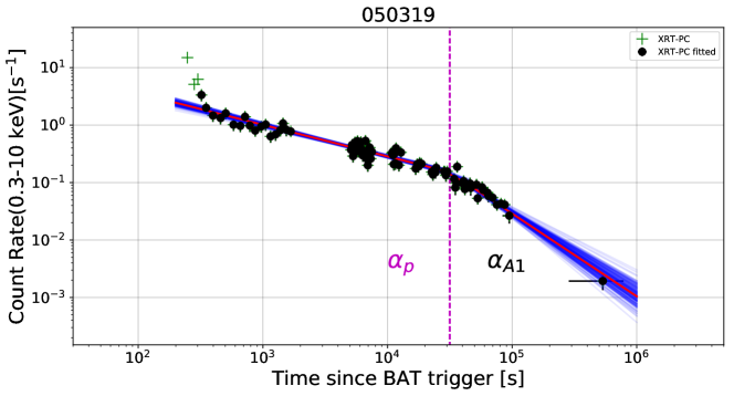
b

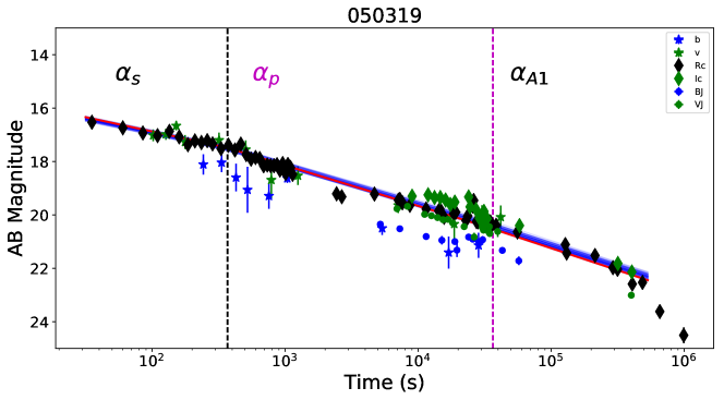
Supplementary Figure 1: (a) The X-ray LC of GRB 050319. The green crosses represent the XRT-PC mode data which are excluded from the fit. The black dots represent XRT-PC mode fitted data. The errors correspond to a significance of one sigma. The dashed vertical (purple) line represents the break times $T_{\rm a}$ (at the end of the plateau phase). The $\alpha_{\rm p}$ and $\alpha_{\rm A1}$ are the slopes during the plateau phase and the self-similar phase respectively. (b) The optical LC of GRB 050319. The blue and green colors together with stars, diamonds and dots represent the data in b, v, Rc, Ic, BJ, VJ bands respectively. The errors correspond to a significance of one sigma. For the details of the excluded data, see, Supplementary Method Supplementary Method 1b. Optical data and fitting process. Although all the bands are jointly fitted, for the demonstration purpose, only the Rc band fit result is displayed. The dashed vertical lines (black and purple) represent the break times $T_{\rm s}$ and $T_{\rm a}$ (at the end of the plateau phase) respectively. The $\alpha_{\rm As}$, $\alpha_{\rm p}$, $\alpha_{\rm A1}$, are the slopes before the plateau phase, during the plateau phase and self-similar phase respectively. In both panels (a) and (b), the red line shows the mean of the posterior distribution and blue lines are 200 randomly selected samples from the MCMC sampling.

a
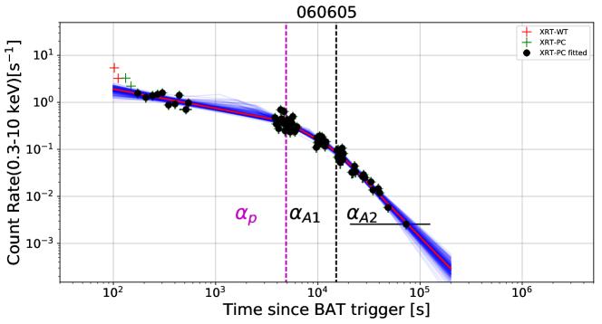
b

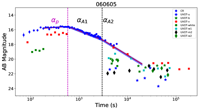
Supplementary Figure 2: (a) The X-ray LC of GRB 060605. The red and green crosses represent the XRT-WT and the XRT-PC mode data respectively which are excluded from the fit. The black dots represent the XRT-PC mode fitted data. The errors correspond to a significance of one sigma. (b) The optical LC of GRB 060605. The blue, green, red, cyan, black colors together with points, stars, squares diamonds represent the data in CR, UVOT-u, UVOT-b, UVOT-v, UVOT-white, UVOT-w1, UVOT-m2, UVOT-w2 bands respectively. The errors correspond to a significance of one sigma. For the details of the excluded data, see, Supplementary Method Supplementary Method 1b. Optical data and fitting process. Although all the bands jointly fitted, for the demonstration purpose only CR band fit result displayed. In both panels (a) and (b), the red line shows the mean of the posterior distribution and blue lines are 200 randomly selected samples from the MCMC sampling. The dashed vertical lines (purple and black) represent the break times $T_{\rm a}$ (at the end of the plateau phase) and $T_{\rm b}$ respectively. The $\alpha_{\rm p}$, $\alpha_{\rm A1}$, $\alpha_{\rm A2}$ are slopes during the plateau phase, self-similar phase and after the jet break time respectively.

a
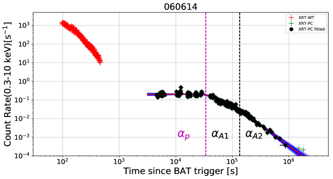
b

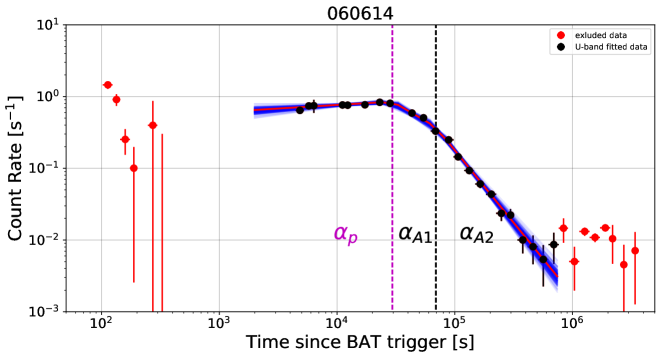
Supplementary Figure 3: (a) The X-ray LC of GRB 060614. The red and green crosses represent the XRT-WT and the XRT-PC mode data respectively which are excluded from the fit. The black dots represent the XRT-PC mode fitted data. The errors correspond to a significance of one sigma. (b) The optical LC of GRB 060614. The black and red dots represent the data in UVOT-u band. The errors correspond to a significance of one sigma. While the black dots are considered in the fitting process, the red dots are excluded from the fit (see, Supplementary Method Supplementary Method 1b. Optical data and fitting process for explanations). In both panels (a) and (b), the red line shows the mean of the posterior distribution and blue lines are 200 randomly selected samples from the MCMC sampling. The dashed vertical lines (purple and black) represent the break times $T_{\rm a}$ (at the end of the plateau phase) and $T_{\rm b}$ respectively. The $\alpha_{\rm p}$, $\alpha_{\rm A1}$, $\alpha_{\rm A2}$ are slopes during the plateau phase, self-similar phase and after the jet break time respectively.

a
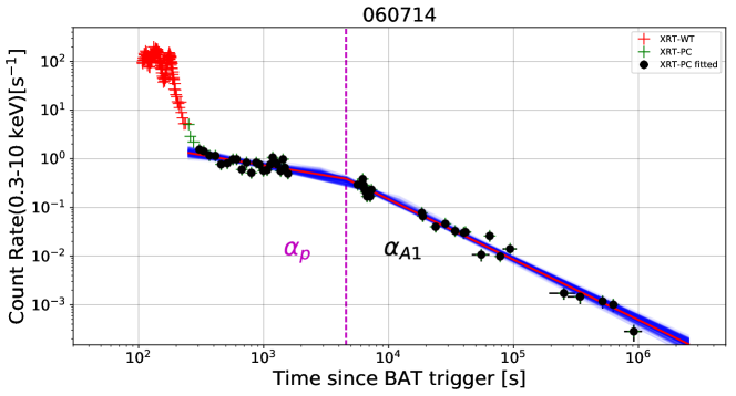
b

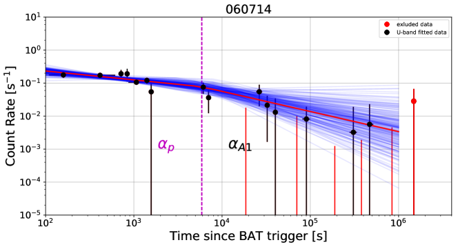
Supplementary Figure 4: (a) The X-ray LC of GRB 060714. The red and green crosses represent the XRT-WT and the XRT-PC mode data respectively which are excluded from the fit. The black dots represent the XRT-PC mode fitted data. The errors correspond to a significance of one sigma. (b) The optical LC of GRB 060714. The black and red dots represent the data in UVOT-u band. The errors correspond to a significance of one sigma. While the black dots are considered in the fitting process, the red dots are excluded from the fit (see, Supplementary Method Supplementary Method 1b. Optical data and fitting process for explanations). In both panels (a) and (b), the red line shows the mean of the posterior distribution and blue lines are 200 randomly selected samples from the MCMC sampling. The dashed vertical line (purple) represents the break times $T_{\rm a}$ (at the end of the plateau phase). The $\alpha_{\rm p}$, $\alpha_{\rm A1}$ are slopes during the plateau phase and self-similar phase respectively.

a
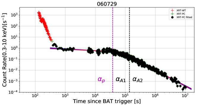
b

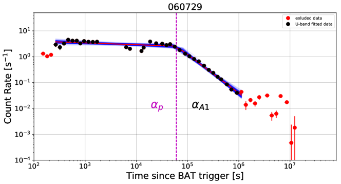
Supplementary Figure 5: (a) The X-ray LC of GRB 060614. The red and green crosses represent the XRT-WT and the XRT-PC mode data respectively which are excluded from the fit. The black dots represent the XRT-PC mode fitted data. The errors correspond to a significance of one sigma. The dashed vertical lines (purple and black) represent the break times $T_{\rm a}$ (at the end of the plateau phase) and $T_{\rm b}$ respectively. The $\alpha_{\rm p}$, $\alpha_{\rm A1}$, $\alpha_{\rm A2}$ are slopes during the plateau phase, self-similar phase and after the jet break time respectively. (b) The optical LC of GRB 060614. The black and red dots represent the data in UVOT-u band. The errors correspond to a significance of one sigma. While the black dots are considered in the fitting process, the red dots are excluded from the fit (see, Supplementary Method Supplementary Method 1b. Optical data and fitting process for explanations). The dashed vertical line (purple) represents the break times $T_{\rm a}$ (at the end of the plateau phase). The $\alpha_{\rm p}$, $\alpha_{\rm A1}$ are slopes during the plateau phase and self-similar phase respectively. In both panels (a) and (b), the red line shows the mean of the posterior distribution and blue lines are 200 randomly selected samples from the MCMC sampling.

a
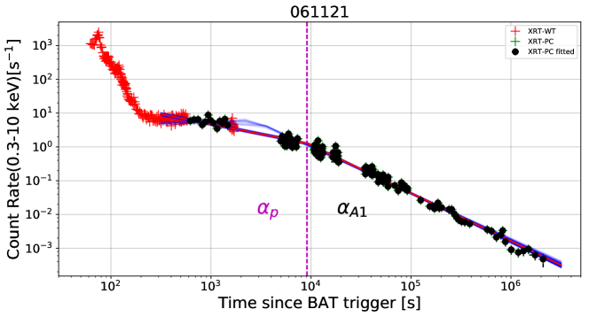
b

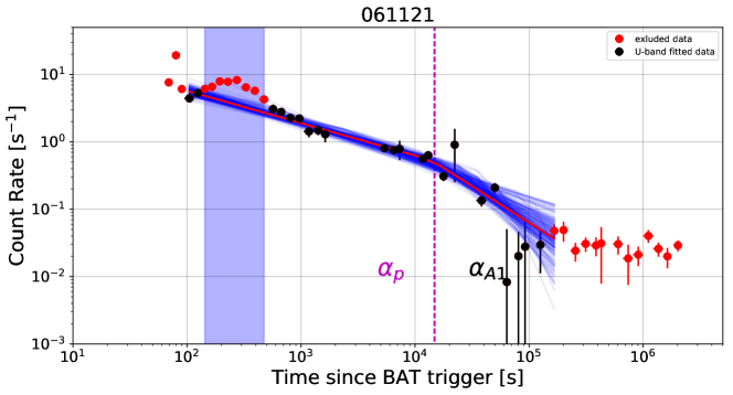
Supplementary Figure 6: (a) The X-ray LC of GRB 061121. The red crosses represent the XRT-WT mode data which are excluded from the fit. The black dots represent the XRT-PC mode fitted data. The errors correspond to a significance of one sigma. (b) The optical LC of GRB 061121. The black and red dots represent the data in UVOT-u band.The errors correspond to a significance of one sigma. While the black dots are considered in the fitting process, the red dots (including blue shaded region) are excluded from the fit (see, Supplementary Method Supplementary Method 1b. Optical data and fitting process for explanations). In both panels (a) and (b), the red line shows the mean of the posterior distribution and blue lines are 200 randomly selected samples from the MCMC sampling. The dashed vertical line (purple) represents the break times $T_{\rm a}$ (at the end of the plateau phase). The $\alpha_{\rm p}$, $\alpha_{\rm A1}$ are slopes during the plateau phase and self-similar phase respectively.

a
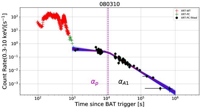
b

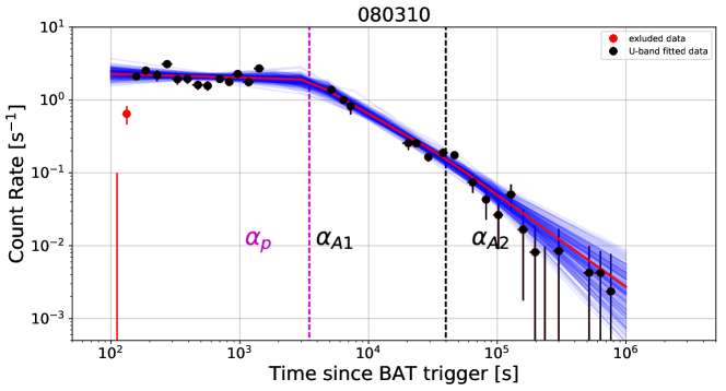
Supplementary Figure 7: (a) The X-ray LC of GRB 061121. The red crosses represent the XRT-WT and XRT-PC mode data respectively which are excluded from the fit. The black dots represent the XRT-PC mode fitted data. The errors correspond to a significance of one sigma. The dashed vertical line (purple) represents the break times $T_{\rm a}$ (at the end of the plateau phase). The $\alpha_{\rm p}$, $\alpha_{\rm A1}$ are slopes during the plateau phase and self-similar phase respectively. (b) The optical LC of GRB 061121. The black and red dots represent the data in UVOT-u band. The errors correspond to a significance of one sigma. While the black dots are considered in the fitting process, the red dots (including blue shaded region) are excluded from the fit (see, Supplementary Method Supplementary Method 1b. Optical data and fitting process for explanations). The dashed vertical lines (purple and black) represent the break times $T_{\rm a}$ (at the end of the plateau phase) and $T_{\rm b}$ respectively. The $\alpha_{\rm p}$, $\alpha_{\rm A1}$, $\alpha_{\rm A2}$ are slopes during the plateau phase, self-similar phase and after the jet break time respectively. In both panels (a) and (b), the red line shows the mean of the posterior distribution and blue lines are 200 randomly selected samples from the MCMC sampling.

a
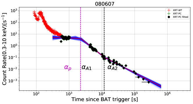
b

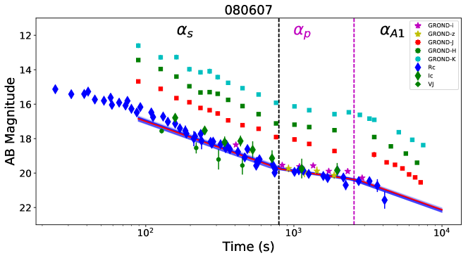
Supplementary Figure 8: (a) The X-ray LC of GRB 080607. The red crosses represent the XRT-WT mode data which are excluded from the fit. The black dots represent XRT-PC mode fitted data. The errors correspond to a significance of one sigma. The dashed vertical lines (purple and black) represent the break times $T_{\rm a}$ (at the end of the plateau phase) and $T_{\rm b}$ respectively. The $\alpha_{\rm p}$, $\alpha_{\rm A1}$, $\alpha_{\rm A2}$ are slopes during the plateau phase, self-similar phase and after the jet break time respectively. (b) The optical LC of GRB 080607. The purple, yellow, red, green, cyan, blue, black colors together with stars, squares, diamonds and point represent the data in GROND-i, GROND-z, GROND-J, GROND-H, GROND-K, Rc, Ic, VJ bands respectively. The errors correspond to a significance of one sigma. For the details of the excluded data, see, Supplementary Method Supplementary Method 1b. Optical data and fitting process. Although all the bands are jointly fitted, for the demonstration purpose, only the Rc band fit result is displayed. The dashed vertical lines (black and purple) represent the break times $T_{\rm s}$ and $T_{\rm a}$ (at the end of the plateau phase) respectively. The $\alpha_{\rm As}$, $\alpha_{\rm p}$, $\alpha_{\rm A1}$, are the slopes before the plateau phase, during the plateau phase and self-similar phase respectively. In both panels (a) and (b), the red line shows the mean of the posterior distribution and blue lines are 200 randomly selected samples from the MCMC sampling.

a
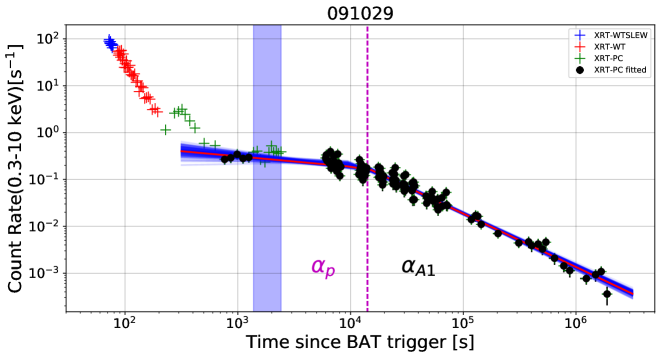
b

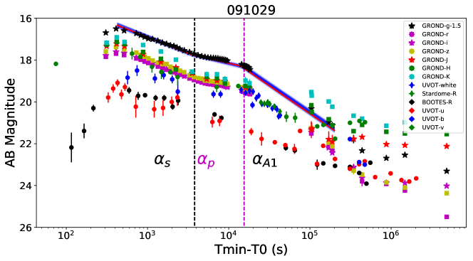
Supplementary Figure 9: (a) The X-ray LC of GRB 091029. The blue, red and green crosses represent the XRT-WTSLEW, XRT-WT, XRT-PC (including blue shaded region, see, Supplementary Method Supplementary Method 1a. X-ray data and fitting process for explanation) mode data which are excluded from the fit. The black dots represent XRT-PC mode fitted data. The errors correspond to a significance of one sigma. The dashed vertical line (purple) represents the break times $T_{\rm a}$ (at the end of the plateau phase). The $\alpha_{\rm p}$, $\alpha_{\rm A1}$ are slopes during the plateau phase and self-similar phase respectively. (b) The optical LC of GRB 091029. The black, purple, yellow, red, green, cyan, blue, black colors together with stars, squares, diamonds and points represent the data in GROND-g, GROND-r, GROND-i, GROND-z, GROND-J, GROND-H, GROND-K, UVOT-white, Stardome-R, BOOTES-R, UVOT-u, UVOT-b, UVOT-v bands respectively. The errors correspond to a significance of one sigma. For the details of the excluded data, see, Supplementary Method Supplementary Method 1b. Optical data and fitting process. Although all the bands are jointly fitted, for the demonstration purpose, only the GROND-g band fit result is displayed and GROND-g band light curve distinguished by subtracting 1.5 from the AB magnitude. The dashed vertical lines (black and purple) represent the break times $T_{\rm s}$ and $T_{\rm a}$ (at the end of the plateau phase) respectively. The $\alpha_{\rm As}$, $\alpha_{\rm p}$, $\alpha_{\rm A1}$, are the slopes before the plateau phase, during the plateau phase and self-similar phase respectively. In both panels (a) and (b), the red line shows the mean of the posterior distribution and blue lines are 200 randomly selected samples from the MCMC sampling.

a
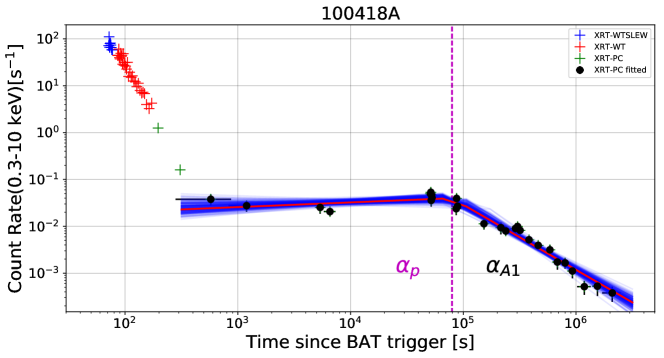
b

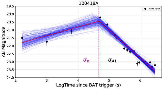
Supplementary Figure 10: (a) The X-ray LC of GRB 100418A. The blue, red and green crosses represent the XRT-WTSLEW, XRT-WT, XRT-PC mode data which are excluded from the fit. The black dots represent XRT-PC mode fitted data. The errors correspond to a significance of one sigma. (b) The optical LC of GRB 100418A. The black points represent the data in UVOT-white band. The errors correspond to a significance of one sigma. In both panels (a) and (b), the red line shows the mean of the posterior distribution and blue lines are 200 randomly selected samples from the MCMC sampling. The dashed vertical line (purple) represents the break times $T_{\rm a}$ (at the end of the plateau phase). The $\alpha_{\rm p}$, $\alpha_{\rm A1}$ are slopes during the plateau phase and self-similar phase respectively.

a
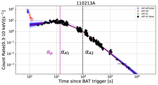
b

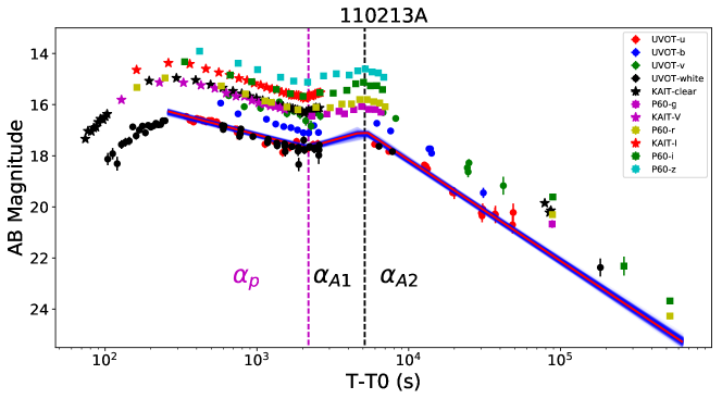
Supplementary Figure 11: (a) The X-ray LC of GRB 110213A. The blue, red and green crosses represent the XRT-WTSLEW and XRT-WT mode data respectively which are excluded from the fit. The black dots represent the XRT-PC mode fitted data. The errors correspond to a significance of one sigma. (b) The optical LC of GRB 110213A. The red, blue, green, black, purple, yellow, cyan colors together with points, stars, squares represent the data in UVOT-u, UVOT-b, UVOT-v, UVOT-white, KAIT-clear, P60-g, KAIT-V, P60-r, KAIT-I, P60-i, P60-z bands respectively. The errors correspond to a significance of one sigma. For the details of the excluded data, see, Supplementary Method Supplementary Method 1b. Optical data and fitting process. Although all the bands jointly fitted, for the demonstration purpose only UVOT-u band fit result displayed. In both panels (a) and (b), The red line shows the mean of the posterior distribution and blue lines are 200 randomly selected samples from the MCMC sampling. The dashed vertical lines (purple and black) represent the break times $T_{\rm a}$ (at the end of the plateau phase) and $T_{\rm b}$ respectively. The $\alpha_{\rm p}$, $\alpha_{\rm A1}$, $\alpha_{\rm A2}$ are slopes during the plateau phase, self-similar phase and after the jet break time respectively.

a
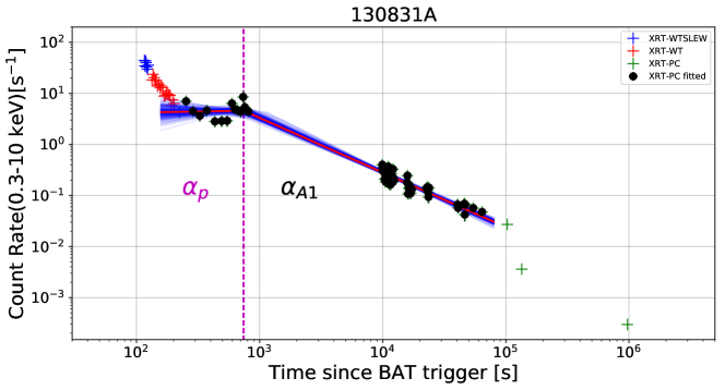
b

Supplementary Figure 12: (a) The X-ray LC of GRB 130831A. The blue, red and green crosses represent the XRT-WTSLEW, XRT-WT, XRT-PC mode data which are excluded from the fit. The black dots represent XRT-PC mode fitted data. The errors correspond to a significance of one sigma. (b) The optical LC of GRB 130831A. The purple, yellow, red, green, blue, black, cyan colors together with squares, stars and points represent the data in GROND-r, GROND-i, GROND-z, GROND-J, GROND-H, Rc, B, V, Ic, UVOT-u, UVOT-b, UVOT-v and CR bands respectively. The errors correspond to a significance of one sigma. The data marked by blue shaded region excluded from the fit, see, Supplementary Method Supplementary Method 1b. Optical data and fitting process for explanation. Although all the bands jointly fitted, for the demonstration purpose only UVOT-u band fit result displayed. In both panels (a) and (b), the red line shows the mean of the posterior distribution and blue lines are 200 randomly selected samples from the MCMC sampling. The dashed vertical line (purple) represents the break times $T_{\rm a}$ (at the end of the plateau phase). The $\alpha_{\rm p}$, $\alpha_{\rm A1}$ are slopes during the plateau phase and self-similar phase respectively.

a
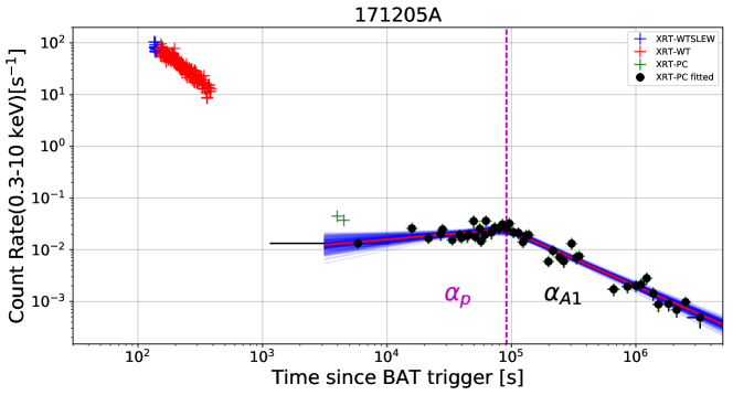
b

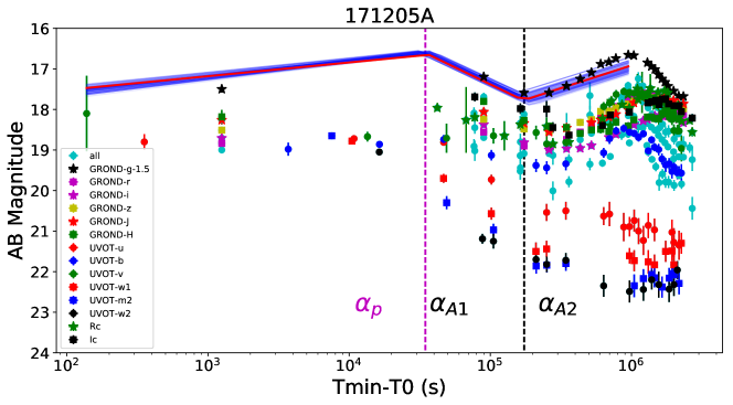
Supplementary Figure 13: (a) The X-ray LC of GRB 171205A. The blue, red and green crosses represent the XRT-WTSLEW, XRT-WT, XRT-PC mode data which are excluded from the fit. The black dots represent XRT-PC mode fitted data. The errors correspond to a significance of one sigma. The dashed vertical line (purple) represents the break times $T_{\rm a}$ (at the end of the plateau phase). The $\alpha_{\rm p}$, $\alpha_{\rm A1}$ are slopes during the plateau phase and self-similar phase respectively. (b) The optical LC of GRB 171205A. The black, purple, yellow, red, green, blue colors together with points, stars, squares represent the data GROND-g, GROND-r, GROND-i, GROND-z, GROND-J, GROND-H, UVOT-u, UVOT-b, UVOT-v, UVOT-w1, UVOT-m2, UVOT-w2, Rc, Ic bands respectively. The errors correspond to a significance of one sigma. The cyan colors represent the other data that are not considered in the fitting process. For the details of the excluded data, see, Supplementary Method Supplementary Method 1b. Optical data and fitting process. Although all the bands are jointly fitted, for the demonstration purpose, only the GROND-g band fit result is displayed and GROND-g band light curve distinguished by subtracting 1.5 from the AB magnitude. The dashed vertical lines (black and purple) represent the break times $T_{\rm s}$ and $T_{\rm a}$ (at the end of the plateau phase) respectively. The $\alpha_{\rm As}$, $\alpha_{\rm p}$, $\alpha_{\rm A1}$, are the slopes before the plateau phase, during the plateau phase and self-similar phase respectively. In both panels (a) and (b), the red line shows the mean of the posterior distribution and blue lines are 200 randomly selected samples from the MCMC sampling.

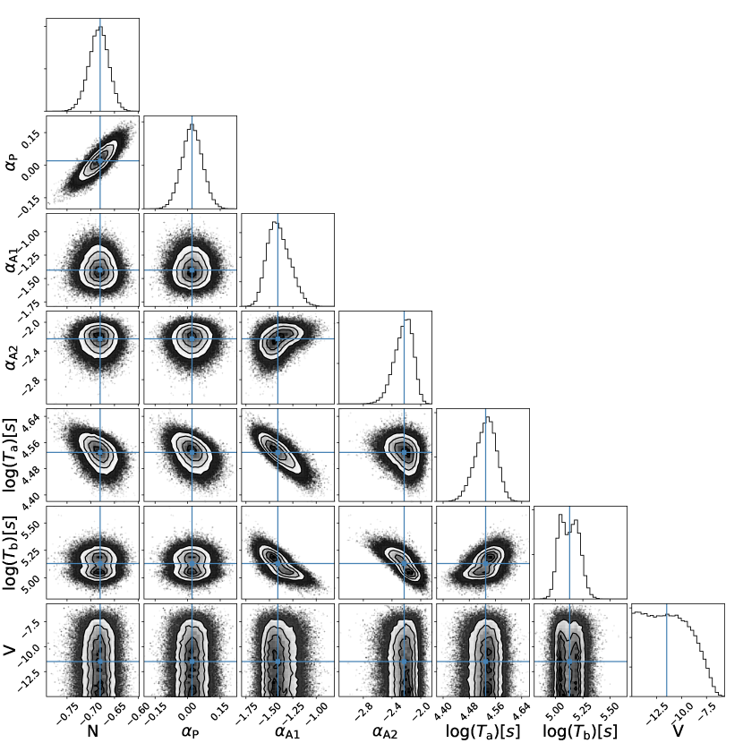
Supplementary Figure 14: Corner plot showing the one-and two-dimensional posterior probability distributions for the fit parameters obtained from the X-ray LC of GRB 060614. The blue lines present the mean value of each parameter given in Table 4. Contours gives from inward to outward 39.3%, 68.3% ,90.3% confidence region.

a	b

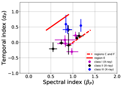
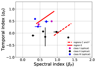
Supplementary Figure 15: Temporal and spectral indices of the 13 GRBs in our sample during the plateau phase (a) in the X-ray band and (b) in the optical band. The purple, black, and blue data points correspond to the three classes (I, II and III respectively). The errors correspond to a significance of one sigma. The spectral indices in the optical band of GRBs 100418A (in class II), 110213A and 130831A (both in class I) during the plateau phase could not be retrieved from the literature, and therefore these GRBs are excluded from panel (b). The red line shows the closure relation obtained for region E in which $\nu_{m}<\nu_{\rm obs.}<\nu_{c}$, and the dashed red line represents regions C and F in which $\nu_{c}<\nu_{m}<\nu_{\rm obs.}$ and $\nu_{m}<\nu_{c}<\nu_{\rm obs.}$ respectively. These lines are computed by using an electron power-law index $p=1.8-2.8$. Despite the simplicity of the model, most data points are in between the expected theoretical limits in both X-ray and optic bands. The source data necessary to reproduce this Figure are provided as a Source Data file.

a	b

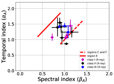
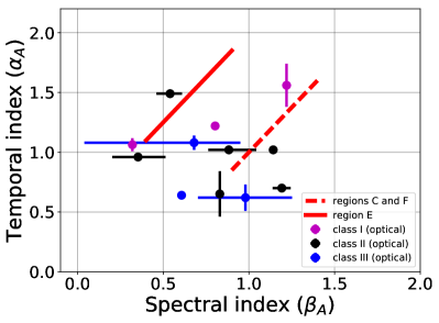
Supplementary Figure 16: Temporal and spectral indices of the 13 GRBs during the self-similar phase (a) in the X-ray band and (b) in the optical band. The spectral index in the optical band of 130831A (in class I) during the self-similar phase could not be retrieved from the literature, and therefore this GRB is excluded from panel (b). The color coding is as in Supplementary Fig. 15 for the data points and regions. In the X-ray band, all the data points are within the expected theoretical limits of the closure relations of the model during this phase as well, while in the optical band, where the spectral indices are taken from the literature, the scatter is larger. The source data necessary to reproduce this Figure are provided as a Source Data file.

a	b
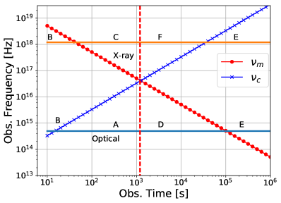
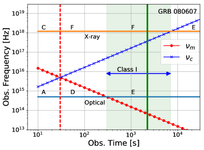
c	d

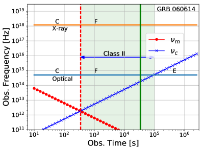
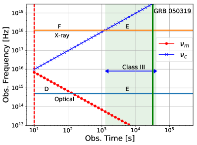
Supplementary Figure 17: Temporal evolution of the injection frequency, $\nu_{m}$ (red points) and of the cooling frequency $\nu_{c}$ (blue crosses) in the coasting phase into a wind medium. The letters (A, B, C, D, E, F) represent the six possible spectral and temporal regions given in Table 5 and by Supplementary Equations (4) and (5). The orange and blue horizontal lines represent the X-ray and optical frequencies respectively. The red dashed vertical line indicates the crossing of the injection and of the cooling frequencies. It is clear that a given observed frequency can shift from one region to another only along one of the following paths: i) B-C-F-E or ii) B-A-D-E. Panel (a) is an illustration while panels (b), (c) and (d) are three examples showing the occupied region (green vertical span) of the light curves of GRBs 080607, 060614, 050319 obtained from X-ray (in region F, F, E respectively) and optical data (in region E, F, E). The color coding is as in panel (a), except that the green vertical line shows $T_{\rm a,X}$, the time marking the end of the plateau phase. The characteristic frequencies $\nu_{m}$ and $\nu_{c}$ are computed using the outflow parameters of GRBs 080607, 060614, 050319 presented in Table 3 (main text). Clearly, during most of the plateau as well as the early afterglow phases, GRBs 080607, 060614, 050319 are classified as being in class I, II, III respectively.

References

- [1] Krolik, J. H. & Pier, E. A. Relativistic motion in gamma-ray bursts. ApJ 373, 277–284, DOI: 10.1086/170048 (1991).
- [2] Fenimore, E. E., Epstein, R. I. & Ho, C. The escape of 100 MeV photons from cosmological gamma-ray bursts. A&AS 97, 59–62 (1993).
- [3] Racusin, J. L. et al. Fermi and Swift Gamma-ray Burst Afterglow Population Studies. ApJ 738, 138, DOI: 10.1088/0004-637X/738/2/138 (2011). 1106.2469.
- [4] Nousek, J. A. et al. Evidence for a Canonical Gamma-Ray Burst Afterglow Light Curve in the Swift XRT Data. ApJ 642, 389–400, DOI: 10.1086/500724 (2006). astro-ph/0508332.
- [5] O’Brien, P. T. et al. The Early X-Ray Emission from GRBs. ApJ 647, 1213–1237, DOI: 10.1086/505457 (2006). astro-ph/0601125.
- [6] Zhang, B. et al. Physical Processes Shaping Gamma-Ray Burst X-Ray Afterglow Light Curves: Theoretical Implications from the Swift X-Ray Telescope Observations. ApJ 642, 354–370, DOI: 10.1086/500723 (2006). astro-ph/0508321.
- [7] Srinivasaragavan, G. P. et al. On the Investigation of the Closure Relations for Gamma-Ray Bursts Observed by Swift in the Post-plateau Phase and the GRB Fundamental Plane. ApJ 903, 18, DOI: 10.3847/1538-4357/abb702 (2020). 2009.06740.
- [8] Evans, P. A. et al. Methods and results of an automatic analysis of a complete sample of Swift-XRT observations of GRBs. MNRAS 397, 1177–1201, DOI: 10.1111/j.1365-2966.2009.14913.x (2009). 0812.3662.
- [9] Meszaros, P. & Rees, M. J. Relativistic fireballs and their impact on external matter - Models for cosmological gamma-ray bursts. ApJ 405, 278–284, DOI: 10.1086/172360 (1993).
- [10] Gehrels, N. et al. The Swift Gamma-Ray Burst Mission. ApJ 611, 1005–1020, DOI: 10.1086/422091 (2004). astro-ph/0405233.
- [11] Granot, J. & Kumar, P. Distribution of gamma-ray burst ejecta energy with Lorentz factor. MNRAS 366, L13–L16, DOI: 10.1111/j.1745-3933.2005.00121.x (2006). astro-ph/0511049.
- [12] Metzger, B. D., Giannios, D., Thompson, T. A., Bucciantini, N. & Quataert, E. The protomagnetar model for gamma-ray bursts. MNRAS 413, 2031–2056, DOI: 10.1111/j.1365-2966.2011.18280.x (2011). 1012.0001.
- [13] Berger, E. et al. A common origin for cosmic explosions inferred from calorimetry of GRB030329. Nature 426, 154–157, DOI: 10.1038/nature01998 (2003). astro-ph/0308187.
- [14] Huang, Y. F., Wu, X. F., Dai, Z. G., Ma, H. T. & Lu, T. Rebrightening of XRF 030723: Further Evidence for a Two-Component Jet in a Gamma-Ray Burst. ApJ 605, 300–306, DOI: 10.1086/382202 (2004). astro-ph/0309360.
- [15] Granot, J., Königl, A. & Piran, T. Implications of the early X-ray afterglow light curves of Swift gamma-ray bursts. MNRAS 370, 1946–1960, DOI: 10.1111/j.1365-2966.2006.10621.x (2006). astro-ph/0601056.
- [16] Toma, K., Ioka, K., Yamazaki, R. & Nakamura, T. Shallow Decay of Early X-Ray Afterglows from Inhomogeneous Gamma-Ray Burst Jets. ApJ 640, L139–L142, DOI: 10.1086/503384 (2006). astro-ph/0511718.
- [17] Ioka, K., Toma, K., Yamazaki, R. & Nakamura, T. Efficiency crisis of swift gamma-ray bursts with shallow X-ray afterglows: prior activity or time-dependent microphysics? A&A 458, 7–12, DOI: 10.1051/0004-6361:20064939 (2006). astro-ph/0511749.
- [18] Shao, L. & Dai, Z. G. Behavior of X-Ray Dust Scattering and Implications for X-Ray Afterglows of Gamma-Ray Bursts. ApJ 660, 1319–1325, DOI: 10.1086/513139 (2007). astro-ph/0703009.
- [19] Uhm, Z. L. & Beloborodov, A. M. On the Mechanism of Gamma-Ray Burst Afterglows. ApJ 665, L93–L96, DOI: 10.1086/519837 (2007). astro-ph/0701205.
- [20] Genet, F., Daigne, F. & Mochkovitch, R. Can the early X-ray afterglow of gamma-ray bursts be explained by a contribution from the reverse shock? MNRAS 381, 732–740, DOI: 10.1111/j.1365-2966.2007.12243.x (2007). astro-ph/0701204.
- [21] Eichler, D. & Granot, J. The Case for Anisotropic Afterglow Efficiency within Gamma-Ray Burst Jets. ApJ 641, L5–L8, DOI: 10.1086/503667 (2006). astro-ph/0509857.
- [22] Eichler, D. Cloaked Gamma-Ray Bursts. ApJ 787, L32, DOI: 10.1088/2041-8205/787/2/L32 (2014). 1402.0245.
- [23] Kumar, P. & Zhang, B. The physics of gamma-ray bursts and relativistic jets. Phys. Rep. 561, 1–109, DOI: 10.1016/j.physrep.2014.09.008 (2015). 1410.0679.
- [24] Kouveliotou, C. et al. Identification of Two Classes of Gamma-Ray Bursts. ApJ 413, L101, DOI: 10.1086/186969 (1993).
- [25] Eichler, D., Livio, M., Piran, T. & Schramm, D. N. Nucleosynthesis, neutrino bursts and -rays from coalescing neutron stars. Nature 340, 126–128, DOI: 10.1038/340126a0 (1989).
- [26] Woosley, S. E. Gamma-Ray Bursts from Stellar Mass Accretion Disks around Black Holes. ApJ 405, 273, DOI: 10.1086/172359 (1993).
- [27] MacFadyen, A. I. & Woosley, S. E. Collapsars: Gamma-Ray Bursts and Explosions in “Failed Supernovae”. ApJ 524, 262–289, DOI: 10.1086/307790 (1999). astro-ph/9810274.
- [28] Galama, T. J. et al. An unusual supernova in the error box of the -ray burst of 25 April 1998. Nature 395, 670–672, DOI: 10.1038/27150 (1998). astro-ph/9806175.
- [29] Hjorth, J. et al. A very energetic supernova associated with the -ray burst of 29 March 2003. Nature 423, 847–850, DOI: 10.1038/nature01750 (2003). astro-ph/0306347.
- [30] Woosley, S. E. & Bloom, J. S. The Supernova Gamma-Ray Burst Connection. ARA&A 44, 507–556, DOI: 10.1146/annurev.astro.43.072103.150558 (2006). astro-ph/0609142.
- [31] Fruchter, A. S. et al. Long -ray bursts and core-collapse supernovae have different environments. Nature 441, 463–468, DOI: 10.1038/nature04787 (2006). astro-ph/0603537.
- [32] Modjaz, M. et al. Measured Metallicities at the Sites of Nearby Broad-Lined Type Ic Supernovae and Implications for the Supernovae Gamma-Ray Burst Connection. AJ 135, 1136–1150, DOI: 10.1088/0004-6256/135/4/1136 (2008). astro-ph/0701246.
- [33] Vink, J. S. & de Koter, A. On the metallicity dependence of Wolf-Rayet winds. A&A 442, 587–596, DOI: 10.1051/0004-6361:20052862 (2005). astro-ph/0507352.
- [34] Sari, R., Piran, T. & Narayan, R. Spectra and Light Curves of Gamma-Ray Burst Afterglows. ApJ 497, L17+, DOI: 10.1086/311269 (1998). arXiv:astro-ph/9712005.
- [35] Santana, R., Barniol Duran, R. & Kumar, P. Magnetic Fields in Relativistic Collisionless Shocks. ApJ 785, 29, DOI: 10.1088/0004-637X/785/1/29 (2014). 1309.3277.
- [36] Barniol Duran, R. Constraining the magnetic field in GRB relativistic collisionless shocks using radio data. MNRAS 442, 3147–3154, DOI: 10.1093/mnras/stu1070 (2014). 1311.1216.
- [37] Wang, X.-Y., Liu, R.-Y. & Lemoine, M. On the Origin of > 10 GeV Photons in Gamma-Ray Burst Afterglows. ApJ 771, L33, DOI: 10.1088/2041-8205/771/2/L33 (2013). 1305.1494.
- [38] Nava, L. et al. Constraints on the bulk Lorentz factor of gamma-ray burst jets from Fermi /LAT upper limits. MNRAS 465, 811–819, DOI: 10.1093/mnras/stw2771 (2017). 1610.08056.
- [39] Piran, T. Gamma-ray bursts and the fireball model. Phys. Rep. 314, 575–667, DOI: 10.1016/S0370-1573(98)00127-6 (1999). astro-ph/9810256.
- [40] Daigne, F. & Mochkovitch, R. The expected thermal precursors of gamma-ray bursts in the internal shock model. MNRAS 336, 1271–1280, DOI: 10.1046/j.1365-8711.2002.05875.x (2002). astro-ph/0207456.
- [41] Golkhou, V. Z. & Butler, N. R. Uncovering the Intrinsic Variability of Gamma-Ray Bursts. ApJ 787, 90, DOI: 10.1088/0004-637X/787/1/90 (2014). 1403.4254.
- [42] Sonbas, E. et al. Gamma-ray Bursts: Temporal Scales and the Bulk Lorentz Factor. ApJ 805, 86, DOI: 10.1088/0004-637X/805/2/86 (2015). 1408.3042.
- [43] Dainotti, M. G. et al. On the Existence of the Plateau Emission in High-energy Gamma-Ray Burst Light Curves Observed by Fermi-LAT. ApJS 255, 13, DOI: 10.3847/1538-4365/abfe17 (2021). 2105.07357.
- [44] Ajello, M. et al. A Decade of Gamma-Ray Bursts Observed by Fermi-LAT: The Second GRB Catalog. ApJ 878, 52, DOI: 10.3847/1538-4357/ab1d4e (2019). 1906.11403.
- [45] Yamazaki, R., Sato, Y., Sakamoto, T. & Serino, M. Less noticeable shallow decay phase in early X-ray afterglows of GeV/TeV-detected gamma-ray bursts. MNRAS 494, 5259–5269, DOI: 10.1093/mnras/staa1095 (2020). 1910.04097.
- [46] Meszaros, P. & Rees, M. J. Optical and Long-Wavelength Afterglow from Gamma-Ray Bursts. ApJ 476, 232–+, DOI: 10.1086/303625 (1997). arXiv:astro-ph/9606043.
- [47] Zhang, B., Kobayashi, S. & Mészáros, P. Gamma-Ray Burst Early Optical Afterglows: Implications for the Initial Lorentz Factor and the Central Engine. ApJ 595, 950–954, DOI: 10.1086/377363 (2003). astro-ph/0302525.
- [48] Molinari, E. et al. REM observations of GRB 060418 and GRB 060607A: the onset of the afterglow and the initial fireball Lorentz factor determination. A&A 469, L13–L16, DOI: 10.1051/0004-6361:20077388 (2007). astro-ph/0612607.
- [49] Liang, E.-W. et al. Constraining Gamma-ray Burst Initial Lorentz Factor with the Afterglow Onset Feature and Discovery of a Tight 0-Eγ,iso Correlation. ApJ 725, 2209–2224, DOI: 10.1088/0004-637X/725/2/2209 (2010). 0912.4800.
- [50] Burrows, D. N. et al. Bright X-ray Flares in Gamma-Ray Burst Afterglows. Science 309, 1833–1835, DOI: 10.1126/science.1116168 (2005). astro-ph/0506130.
- [51] Chincarini, G. et al. The First Survey of X-Ray Flares from Gamma-Ray Bursts Observed by Swift: Temporal Properties and Morphology. ApJ 671, 1903–1920, DOI: 10.1086/521591 (2007). astro-ph/0702371.
- [52] Falcone, A. D. et al. The First Survey of X-Ray Flares from Gamma-Ray Bursts Observed by Swift: Spectral Properties and Energetics. ApJ 671, 1921–1938, DOI: 10.1086/523296 (2007). 0706.1564.
- [53] Chincarini, G. et al. Unveiling the origin of X-ray flares in gamma-ray bursts. MNRAS 406, 2113–2148, DOI: 10.1111/j.1365-2966.2010.17037.x (2010). 1004.0901.
- [54] Pe’er, A., Ryde, F., Wijers, R. A. M. J., Mészáros, P. & Rees, M. J. A New Method of Determining the Initial Size and Lorentz Factor of Gamma-Ray Burst Fireballs Using a Thermal Emission Component. ApJ 664, L1–L4, DOI: 10.1086/520534 (2007). arXiv:astro-ph/0703734.
- [55] Yu, H.-F., Dereli-Bégué, H. & Ryde, F. Bayesian Time-resolved Spectroscopy of GRB Pulses. ApJ 886, 20, DOI: 10.3847/1538-4357/ab488a (2019). 1810.07313.
- [56] Acuner, Z., Ryde, F., Pe’er, A., Mortlock, D. & Ahlgren, B. The Fraction of Gamma-Ray Bursts with an Observed Photospheric Emission Episode. ApJ 893, 128, DOI: 10.3847/1538-4357/ab80c7 (2020). 2003.06223.
- [57] Dereli-Bégué, H., Pe’er, A. & Ryde, F. Classification of Photospheric Emission in Short GRBs. ApJ 897, 145, DOI: 10.3847/1538-4357/ab9a2d (2020). 2002.06408.
- [58] Virgili, F. J., Qin, Y., Zhang, B. & Liang, E. Spectral and temporal analysis of the joint Swift/BAT-Fermi/GBM GRB sample. MNRAS 424, 2821–2831, DOI: 10.1111/j.1365-2966.2012.21411.x (2012). 1112.4363.
- [59] Zhang, B. et al. GRB Radiative Efficiencies Derived from the Swift Data: GRBs versus XRFs, Long versus Short. ApJ 655, 989–1001, DOI: 10.1086/510110 (2007). astro-ph/0610177.
- [60] Racusin, J. L. et al. Jet Breaks and Energetics of Swift Gamma-Ray Burst X-Ray Afterglows. ApJ 698, 43–74, DOI: 10.1088/0004-637X/698/1/43 (2009). 0812.4780.
- [61] von Kienlin, A. et al. The Fourth Fermi-GBM Gamma-Ray Burst Catalog: A Decade of Data. ApJ 893, 46, DOI: 10.3847/1538-4357/ab7a18 (2020). 2002.11460.
- [62] Chevalier, R. A., Li, Z.-Y. & Fransson, C. The Diversity of Gamma-Ray Burst Afterglows and the Surroundings of Massive Stars. ApJ 606, 369–380, DOI: 10.1086/382867 (2004). astro-ph/0311326.
- [63] Eldridge, J. J., Genet, F., Daigne, F. & Mochkovitch, R. The circumstellar environment of Wolf-Rayet stars and gamma-ray burst afterglows. MNRAS 367, 186–200, DOI: 10.1111/j.1365-2966.2005.09938.x (2006). astro-ph/0509749.
- [64] Crowther, P. A. Physical Properties of Wolf-Rayet Stars. ARA&A 45, 177–219, DOI: 10.1146/annurev.astro.45.051806.110615 (2007). astro-ph/0610356.
- [65] Toalá, J. A. & Guerrero, M. A. Absence of hot gas within the Wolf-Rayet bubble around WR 16. A&A 559, A52, DOI: 10.1051/0004-6361/201322286 (2013). 1309.0236.
- [66] Shen, R. & Matzner, C. D. Coasting External Shock in Wind Medium: An Origin for the X-Ray Plateau Decay Component in Swift Gamma-Ray Burst Afterglows. ApJ 744, 36, DOI: 10.1088/0004-637X/744/1/36 (2012). 1109.3453.
- [67] Dainotti, M. G. et al. The Optical Luminosity-Time Correlation for More than 100 Gamma-Ray Burst Afterglows. ApJ 905, L26, DOI: 10.3847/2041-8213/abcda9 (2020). 2011.14493.
- [68] Valan, V. & Larsson, J. A comprehensive view of blackbody components in the X-ray spectra of GRBs. MNRAS 501, 4974–4997, DOI: 10.1093/mnras/staa3978 (2021). 2101.08296.
- [69] Izzo, L. et al. Signatures of a jet cocoon in early spectra of a supernova associated with a -ray burst. Nature 565, 324–327, DOI: 10.1038/s41586-018-0826-3 (2019). 1901.05500.
- [70] Ghisellini, G., Padovani, P., Celotti, A. & Maraschi, L. Relativistic Bulk Motion in Active Galactic Nuclei. ApJ 407, 65, DOI: 10.1086/172493 (1993).
- [71] Srinivasaragavan, G. P. et al. On the Investigation of the Closure Relations for Gamma-Ray Bursts Observed by Swift in the Post-plateau Phase and the GRB Fundamental Plane. ApJ 903, 18, DOI: 10.3847/1538-4357/abb702 (2020). 2009.06740.
- [72] Dainotti, M. G. et al. The Optical Luminosity-Time Correlation for More than 100 Gamma-Ray Burst Afterglows. ApJ 905, L26, DOI: 10.3847/2041-8213/abcda9 (2020). 2011.14493.
- [73] Dainotti, M. G. et al. The X-Ray Fundamental Plane of the Platinum Sample, the Kilonovae, and the SNe Ib/c Associated with GRBs. The Astrophysical Journal 904, 97, DOI: 10.3847/1538-4357/abbe8a (2020).
- [74] Dainotti, M. G. et al. Closure relations during the plateau emission of Swift GRBs and the fundamental plane. Publications of the Astronomical Society of Japan 73, 970–1000, DOI: 10.1093/pasj/psab057 (2021).
- [75] Dainotti, M. G. et al. On the Existence of the Plateau Emission in High-energy Gamma-Ray Burst Light Curves Observed by Fermi-LAT. The Astrophysical Journal Supplement Series 255, 13, DOI: 10.3847/1538-4365/abfe17 (2021).
- [76] Gehrels, N. et al. The Swift Gamma-Ray Burst Mission. ApJ 611, 1005–1020, DOI: 10.1086/422091 (2004). astro-ph/0405233.
- [77] Dainotti, M. G., Postnikov, S., Hernandez, X. & Ostrowski, M. A Fundamental Plane for Long Gamma-Ray Bursts with X-Ray Plateaus. The Astrophysical Journal 825, L20, DOI: 10.3847/2041-8205/825/2/l20 (2016).
- [78] Dainotti, M. G. et al. A Study of the Gamma-Ray Burst Fundamental Plane. The Astrophysical Journal 848, 88, DOI: 10.3847/1538-4357/aa8a6b (2017).
- [79] Willingale, R. et al. Testing the Standard Fireball Model of Gamma-Ray Bursts Using Late X-Ray Afterglows Measured by Swift. ApJ 662, 1093–1110, DOI: 10.1086/517989 (2007). astro-ph/0612031.
- [80] Zhang, B. et al. Physical Processes Shaping Gamma-Ray Burst X-Ray Afterglow Light Curves: Theoretical Implications from the Swift X-Ray Telescope Observations. ApJ 642, 354–370, DOI: 10.1086/500723 (2006). astro-ph/0508321.
- [81] Ioka, K., Kobayashi, S. & Zhang, B. Variabilities of Gamma-Ray Burst Afterglows: Long-acting Engine, Anisotropic Jet, or Many Fluctuating Regions? ApJ 631, 429–434, DOI: 10.1086/432567 (2005). astro-ph/0409376.
- [82] Boër, M. & Gendre, B. Evidences for two Gamma-Ray Burst afterglow emission regimes. A&A 361, L21–L24 (2000). astro-ph/0008385.
- [83] Gendre, B., Galli, A. & Boër, M. X-Ray Afterglow Light Curves: Toward A Standard Candle? ApJ 683, 620–629, DOI: 10.1086/589805 (2008).
- [84] Oates, S. R. et al. A correlation between the intrinsic brightness and average decay rate of Swift/UVOT gamma-ray burst optical/ultraviolet light curves. MNRAS 426, L86–L90, DOI: 10.1111/j.1745-3933.2012.01331.x (2012). 1208.1856.
- [85] Racusin, J. L., Oates, S. R., de Pasquale, M. & Kocevski, D. A Correlation between the Intrinsic Brightness and Average Decay Rate of Gamma-Ray Burst X-Ray Afterglow Light Curves. ApJ 826, 45, DOI: 10.3847/0004-637X/826/1/45 (2016). 1605.00719.
- [86] Dereli, H. et al. A Study of GRBs with Low-luminosity Afterglows. ApJ 850, 117, DOI: 10.3847/1538-4357/aa947d (2017).
- [87] Lazzati, D. & Perna, R. X-ray flares and the duration of engine activity in gamma-ray bursts. MNRAS 375, L46–L50, DOI: 10.1111/j.1745-3933.2006.00273.x (2007). astro-ph/0610730.
- [88] Evans, P. A. et al. An online repository of Swift/XRT light curves of -ray bursts. A&A 469, 379–385, DOI: 10.1051/0004-6361:20077530 (2007). 0704.0128.
- [89] Evans, P. A. et al. Methods and results of an automatic analysis of a complete sample of Swift-XRT observations of GRBs. MNRAS 397, 1177–1201, DOI: 10.1111/j.1365-2966.2009.14913.x (2009). 0812.3662.
- [90] Goodman, J. & Weare, J. Ensemble samplers with affine invariance. Communications in Applied Mathematics and Computational Science 5, 65–80, DOI: 10.2140/camcos.2010.5.65 (2010).
- [91] Zaninoni, E., Bernardini, M. G., Margutti, R., Oates, S. & Chincarini, G. Gamma-ray burst optical light-curve zoo: comparison with X-ray observations. A&A 557, A12, DOI: 10.1051/0004-6361/201321221 (2013). 1303.6924.
- [92] De Pasquale, M. et al. The central engine of GRB 130831A and the energy breakdown of a relativistic explosion. MNRAS 455, 1027–1042, DOI: 10.1093/mnras/stv2280 (2016). 1509.09234.
- [93] Filgas, R. et al. GRB 091029: at the limit of the fireball scenario. A&A 546, A101, DOI: 10.1051/0004-6361/201219583 (2012). 1209.4658.
- [94] Cucchiara, A. et al. Constraining Gamma-Ray Burst Emission Physics with Extensive Early-time, Multiband Follow-up. ApJ 743, 154, DOI: 10.1088/0004-637X/743/2/154 (2011). 1107.3352.
- [95] de Pasquale, M. et al. VizieR Online Data Catalog: Photometry of the afterglow of GRB 130831A (De Pasquale+, 2016). VizieR Online Data Catalog J/MNRAS/455/1027 (2018).
- [96] Racusin, J. L. et al. Fermi and Swift Gamma-ray Burst Afterglow Population Studies. ApJ 738, 138, DOI: 10.1088/0004-637X/738/2/138 (2011). 1106.2469.
- [97] Oates, S. R. et al. A statistical study of gamma-ray burst afterglows measured by the Swift Ultraviolet Optical Telescope. MNRAS 395, 490–503, DOI: 10.1111/j.1365-2966.2009.14544.x (2009). 0901.3597.
- [98] Zafar, T. et al. The extinction curves of star-forming regions from z = 0.1 to 6.7 using GRB afterglow spectroscopy. A&A 532, A143, DOI: 10.1051/0004-6361/201116663 (2011). 1102.1469.
- [99] Schlegel, D. J., Finkbeiner, D. P. & Davis, M. Maps of Dust Infrared Emission for Use in Estimation of Reddening and Cosmic Microwave Background Radiation Foregrounds. ApJ 500, 525–553, DOI: 10.1086/305772 (1998). astro-ph/9710327.
- [100] Schady, P. et al. Dust and metal column densities in gamma-ray burst host galaxies. MNRAS 401, 2773–2792, DOI: 10.1111/j.1365-2966.2009.15861.x (2010). 0910.2590.
- [101] Pei, Y. C. Interstellar Dust from the Milky Way to the Magellanic Clouds. ApJ 395, 130, DOI: 10.1086/171637 (1992).
- [102] Tang, C.-H., Huang, Y.-F., Geng, J.-J. & Zhang, Z.-B. Statistical Study of Gamma-Ray Bursts with a Plateau Phase in the X-Ray Afterglow. ApJS 245, 1, DOI: 10.3847/1538-4365/ab4711 (2019). 1905.07929.
- [103] Dainotti, M. G., Ostrowski, M. & Willingale, R. Towards a standard gamma-ray burst: tight correlations between the prompt and the afterglow plateau phase emission. Monthly Notices of the Royal Astronomical Society 418, 2202–2206, DOI: 10.1111/j.1365-2966.2011.19433.x (2011). https://academic.oup.com/mnras/article-pdf/418/4/2202/18747557/mnras0418-2202.pdf.
- [104] Dainotti, M. et al. Luminosity–time and luminosity–luminosity correlations for GRB prompt and afterglow plateau emissions. Monthly Notices of the Royal Astronomical Society 451, 3898–3908, DOI: 10.1093/mnras/stv1229 (2015). https://academic.oup.com/mnras/article-pdf/451/4/3898/3889902/stv1229.pdf.
- [105] Dainotti, M. Gamma-ray Burst Correlations. 2053-2563 (IOP Publishing, 2019).
- [106] Spitkovsky, A. On the Structure of Relativistic Collisionless Shocks in Electron-Ion Plasmas. ApJ 673, L39–L42, DOI: 10.1086/527374 (2008). 0706.3126.
- [107] Wijers, R. A. M. J. & Galama, T. J. Physical Parameters of GRB 970508 and GRB 971214 from Their Afterglow Synchrotron Emission. ApJ 523, 177–186, DOI: 10.1086/307705 (1999). astro-ph/9805341.
- [108] Chevalier, R. A. & Li, Z.-Y. Wind Interaction Models for Gamma-Ray Burst Afterglows: The Case for Two Types of Progenitors. ApJ 536, 195–212, DOI: 10.1086/308914 (2000). astro-ph/9908272.
- [109] Blandford, R. D. & McKee, C. F. Fluid dynamics of relativistic blast waves. Physics of Fluids 19, 1130–1138, DOI: 10.1063/1.861619 (1976).
- [110] Pe’er, A. & Wijers, R. A. M. J. The Signature of a Wind Reverse Shock in Gamma-Ray Burst Afterglows. ApJ 643, 1036–1046, DOI: 10.1086/500969 (2006). arXiv:astro-ph/0511508.
- [111] Gao, H., Lei, W.-H., Zou, Y.-C., Wu, X.-F. & Zhang, B. A complete reference of the analytical synchrotron external shock models of gamma-ray bursts. New A Rev. 57, 141–190, DOI: 10.1016/j.newar.2013.10.001 (2013). 1310.2181.
- [112] Metzger, B. D., Giannios, D., Thompson, T. A., Bucciantini, N. & Quataert, E. The protomagnetar model for gamma-ray bursts. MNRAS 413, 2031–2056, DOI: 10.1111/j.1365-2966.2011.18280.x (2011). 1012.0001.
- [113] Rowlinson, A. et al. Constraining properties of GRB magnetar central engines using the observed plateau luminosity and duration correlation. Monthly Notices of the Royal Astronomical Society 443, 1779–1787, DOI: 10.1093/mnras/stu1277 (2014). https://academic.oup.com/mnras/article-pdf/443/2/1779/3703047/stu1277.pdf.
- [114] Rea, N. et al. Constraining the GRB-magnetar model by means of the Galactic pulsar population. The Astrophysical Journal 813, 92, DOI: 10.1088/0004-637x/813/2/92 (2015).
- [115] Stratta, G., Dainotti, M. G., Dall’Osso, S., Hernandez, X. & De Cesare, G. On the Magnetar Origin of the GRBs Presenting X-Ray Afterglow Plateaus. ApJ 869, 155, DOI: 10.3847/1538-4357/aadd8f (2018). 1804.08652.
- [116] Matsumoto, T., Kimura, S. S., Murase, K. & Mészáros, P. Linking extended and plateau emissions of short gamma-ray bursts. MNRAS 493, 783–791, DOI: 10.1093/mnras/staa305 (2020). 2001.09851.
- [117] Bostancı, Z. F., Kaneko, Y. & Göğüş, E. Gamma-ray bursts with extended emission observed with BATSE. MNRAS 428, 1623–1630, DOI: 10.1093/mnras/sts157 (2013). 1210.2399.
- [118] Kaneko, Y., Bostancı, Z. F., Göğüş, E. & Lin, L. Short gamma-ray bursts with extended emission observed with Swift/BAT and Fermi/GBM. MNRAS 452, 824–837, DOI: 10.1093/mnras/stv1286 (2015). 1506.05899.
- [119] Zhao, L. et al. The Second Plateau in X-Ray Afterglow Providing Additional Evidence for Rapidly Spinning Magnetars as the GRB Central Engine. ApJ 896, 42, DOI: 10.3847/1538-4357/ab8f91 (2020). 2005.00768.
- [120] Çıkıntoğlu, S., Şaşmaz Muş, S. & Ekşi, K. Y. The initial evolution of millisecond magnetars: an analytical solution. MNRAS 496, 2183–2190, DOI: 10.1093/mnras/staa1556 (2020). 1910.00554.
- [121] Lyutikov, M. & Camilo Jaramillo, J. Early GRB Afterglows from Reverse Shocks in Ultra-relativistic, Long-lasting Winds. ApJ 835, 206, DOI: 10.3847/1538-4357/835/2/206 (2017). 1612.01162.
- [122] Barkov, M. V., Luo, Y. & Lyutikov, M. Dynamics and Emission of Wind-powered Afterglows of Gamma-Ray Bursts: Flares, Plateaus, and Steep Decays. ApJ 907, 109, DOI: 10.3847/1538-4357/abd5c2 (2021). 2004.13600.
- [123] Genet, F., Daigne, F. & Mochkovitch, R. Can the early X-ray afterglow of gamma-ray bursts be explained by a contribution from the reverse shock? MNRAS 381, 732–740, DOI: 10.1111/j.1365-2966.2007.12243.x (2007). astro-ph/0701204.
- [124] Troja, E. et al. Swift Observations of GRB 070110: An Extraordinary X-Ray Afterglow Powered by the Central Engine. ApJ 665, 599–607, DOI: 10.1086/519450 (2007). astro-ph/0702220.
- [125] Chincarini, G. et al. The First Survey of X-Ray Flares from Gamma-Ray Bursts Observed by Swift: Temporal Properties and Morphology. ApJ 671, 1903–1920, DOI: 10.1086/521591 (2007). astro-ph/0702371.
- [126] Ghisellini, G., Ghirlanda, G., Nava, L. & Firmani, C. “Late Prompt” Emission in Gamma-Ray Bursts? ApJ 658, L75–L78, DOI: 10.1086/515570 (2007). astro-ph/0701430.
- [127] Lü, H.-J., Zhang, B., Lei, W.-H., Li, Y. & Lasky, P. D. The Millisecond Magnetar Central Engine in Short GRBs. ApJ 805, 89, DOI: 10.1088/0004-637X/805/2/89 (2015). 1501.02589.
- [128] Oganesyan, G. et al. Structured Jets and X-Ray Plateaus in Gamma-Ray Burst Phenomena. ApJ 893, 88, DOI: 10.3847/1538-4357/ab8221 (2020). 1904.08786.
- [129] Beniamini, P., Duque, R., Daigne, F. & Mochkovitch, R. X-ray plateaus in gamma-ray bursts’ light curves from jets viewed slightly off-axis. MNRAS 492, 2847–2857, DOI: 10.1093/mnras/staa070 (2020). 1907.05899.
Acknowledgements
We wish to thank Dr. Damien Bégué for enlightening conversations throughout the project as well as Dr. Mukesh Vyas and Dr. Filip Samuelsson for the discussion on the prompt properties of our sample. This work made use of data supplied by the UK Swift Science Data Centre at the University of Leicester. H.D.-B. and A.P. is supported by the European Research Council via ERC consolidating grant 773062 (acronym O.M.J.). F.R. is supported by the Göran Gustafsson Foundation for Research in Natural Sciences and Medicine. We acknowledge support from the Swedish National Space Agency (196/16), the Swedish Research Council (Vetenskapsrådet, 2018-03513), and the Swedish Foundation for international Cooperation in Research and Higher Education (STINT, IB2019-8160).