GRB Radiative Efficiencies Derived from the Swift Data:
GRBs vs. XRFs, Long vs. Short

Abstract

We systematically analyze the prompt emission and the early afterglow data of a sample of 31 GRBs detected by Swift before September 2005, and estimate the GRB radiative efficiency. BAT’s narrow band inhibits a precise determination of the GRB spectral parameters, and we have developed a method to estimate these parameters with the hardness ratio information. The shallow decay component commonly existing in early X-ray afterglows, if interpreted as continuous energy injection in the external shock, suggests that the GRB efficiency previously derived from the late-time X-ray data were not reliable. We calculate two radiative efficiencies using the afterglow kinetic energy $E_{K}$ derived at the putative deceleration time ($t_{\rm dec}$) and at the break time ($t_{b}$) when the energy injection phase ends, respectively. At $t_{b}$ XRFs appear to be less efficient than normal GRBs. However, when we analyze the data at $t_{dec}$ XRFs are found to be as efficient as GRBs. Short GRBs have similar radiative efficiencies to long GRBs despite of their different progenitors. Twenty-two bursts in the sample are identified to have the afterglow cooling frequency below the X-ray band. Assuming $\epsilon_{e}=0.1$, we find $\eta_{\gamma}(t_{b})$ usually $<10\%$ and $\eta_{\gamma}(t_{dec})$ varying from a few percents to $>90\%$. Nine GRBs in the sample have the afterglow cooling frequency above the X-ray band for a very long time. This suggests a very small $\epsilon_{B}$ and/or a very low ambient density $n$.

1 Introduction

Gamma-ray bursts (GRBs) are believed to be the most luminous electromagnetic explosions in the universe. These erratic, transient events in $\gamma$-rays are followed by long-lived, decaying afterglows in longer wavelengths. The widely accepted model of this phenomenon is the fireball model (Mészáros 2002; Zhang & Mészáros 2004; Piran 2005), which depicts the observed prompt gamma-ray emission as the synchrotron emission from the internal shocks in an erratic, unsteady, relativistic fireball (Rees & Mészáros 1994), and interprets the broadband afterglow emission as the synchrotron emission from an external shock that expands into the circumburst medium (Mészáros & Rees 1997; Sari et al. 1998). The GRB radiative efficiency, which is defined as

$$\eta_{\gamma}\equiv\frac{E_{\gamma}}{E_{\gamma}+E_{K}},$$ (1)

is an essential quantity to understand the nature of the bursts. Here $E_{\gamma}$ is the isotropic gamma-ray energy and $E_{K}$ is the isotropic kinetic energy of the fireball right after the prompt gamma-ray emission is over. It gives a direct measure of how efficient the burster dissipates the total energy into radiation during the GRB prompt emission phase.

In the pre-Swift era, only the late time fireball kinetic energy $E_{K}$ was derived or estimated using the late time afterglow data. Two methods have been proposed. The most adequate one is through broadband afterglow modeling (e.g. Panaitescu & Kumar 2001). This method requires well-sampled multi-wavelength afterglow data. The method thus can only be applied to a small sample of GRBs. A more convenient method is to use the X-ray afterglow data alone (Freedman & Waxman 2001; Berger et al. 2003; Lloyd-Ronning & Zhang 2004). At a late enough epoch (e.g. 10 hours after the burst trigger), the X-ray band is likely above the cooling frequency, so that the X-ray flux gives a good measure of the degenerate quantity $\epsilon_{e}E_{K}$, where $\epsilon_{e}$ is the fraction of the electron energy in the internal energy of the shock. If $\epsilon_{e}$ could be estimated, one can then derive $E_{K}$ directly from the X-ray data. Assuming a simple extrapolation of the late time light curve to earlier epochs, Lloyd-Ronning & Zhang (2004) took into account the fireball radiative loss correction to estimate $E_{K}$ right after the prompt emission phase, and estimated the efficiency of 17 GRBs/XRFs observed in the pre-Swift era. They discovered a shallow positive correlation between $\eta_{\gamma}$ and $E_{\gamma}$ or $E_{p}$. According to this shallow correlation, softer, under-luminous bursts (e.g. X-ray flashes) tend to have a lower radiative efficiency. Similar conclusions were also drawn by Lamb et al (2005).

These previous GRB efficiency studies employing the late afterglow data inevitably introduce some uncertainties on the $E_{K}$ measurements, including the possible corrections of radiative fireball energy loss and additional energy injection in the early afterglow phase. In order to reduce these uncertainties very early afterglow observations are needed. The successful operation of NASA’s Swift GRB mission (Gehrels et al. 2004) makes this possible. Very early X-ray afterglow data for a large number of GRBs have been recorded by the X-Ray Telescope (XRT) on board Swift (Burrows et al. 2005a). A large sample of early X-ray afterglow data have been collected, typically 100 seconds after the triggers. These observations indeed show novel, unexpected behaviors in the early afterglow phase (Tagliaferri et al. 2005; Burrows et al. 2005b; Nousek et al. 2006; Zhang et al. 2006; O’Brien et al. 2006), and make it feasible to more robustly estimate $E_{K}$ and hence, $\eta_{\gamma}$.

The XRT light curves of many bursts could be synthesized to a canonical light curve that is composed of 5 components (Zhang et al. 2006), an early rapid decay component consistent with the tail of the prompt emission, a frequently-seen shallow-than-normal decay component likely originated from a refreshed external forward shock, a normal decay component due to a freely expanding fireball, an occasionally-seen post jet break segment, as well as erratic X-ray flares harboring in nearly half of Swift GRBs that are likely due to reactivation of the GRB central engine. The most relevant segment for the efficiency problem is the shallow decay component (Zhang et al. 2006; Nousek et al. 2006). Most of the Swift/XRT afterglow light curves in our sample have such an early shallow decay segment. The origin of this segment is currently not identified. If it is due to continuous energy injection, the initial afterglow energy $E_{K}$ must be significantly smaller than estimated using the late time data. The previous efficiency analysis using late X-ray afterglow data then tend to overestimate $E_{K}$, and hence, underestimate $\eta_{\gamma}$. The early tight UVOT upper limits for many Swift GRBs are also likely related to this shallow decay component (Roming et al. 2006). It is therefore of great interest to revisit the efficiency problem using the very early XRT data.

X-ray flashes (XRFs, Heise et al. 2001; Kippen et al. 2002) naturally extend long-duration GRBs into the softer and fainter regime (e.g. Lamb et al. 2005; Sakamoto et al. 2006). It is now known that the softness of the bursts is not due to their possible high redshifts (Soderberg et al. 2004, 2005). The remaining possibilities include either extrinsic (e.g. viewed at different viewing angles, Yamazaki et al. 2002, 2004; Zhang et al. 2004a,b; Liang & Dai 2004a; Huang et al. 2004), or intrinsic (e.g. different burst parameters such as Lorentz factor, luminosity, etc, Dermer et al. 1999; Kobayashi et al. 2002; Mészáros et al. 2002; Zhang & Mészáros 2002c; Huang et al. 2002; Rees & Mészáros 2005; Barraud et al. 2005) reasons. The radiative efficiency of XRFs may provide a clue to identify the correct mechanism. Previous analyses of late time X-ray data suggest that the XRFs typically have lower radiative efficiencies (Soderberg et al. 2004; Lloyd-Ronning & Zhang 2004; Lamb et al. 2005). It is desirable to investigate whether this is still true with the early afterglow data.

Recently, afterglows of several short-duration GRBs have been detected (Gehrels et al. 2005; Fox et al. 2005; Villasenor et al. 2005; Hjorth et al. 2005; Barthelmy et al. 2005a; Berger et al. 2005c). The data suggest that they are distinct from long GRBs and very likely have different progenitor systems. It is therefore of great interest to explore the radiative efficiencies of short-hard GRBs (SHGs) and compare them with those of long GRBs.

In this paper we systematically analyze the prompt emission and the early afterglow data for a sample of 31 GRBs detected by Swift before September 2005 through reducing the Burst Alert Telescope (BAT, Barthelmy et al. 2005b) and XRT data. We present the sample and the BAT/XRT data analysis methods in §2. The gamma-to-X fluence ratio ($R_{\gamma/X}$) is an observation-defined apparent GRB efficiency indicator. We perform statistical analysis of this parameter in §3. In §4, we perform more detailed theoretical modeling to estimate $E_{K}$ (§4.1) and $\eta_{\gamma}$ (§4.2). Our results are summarized in §5 with some discussion. Throughout the paper the cosmological parameters $H_{0}=71$ km s^-1 Mpc^-1, $\Omega_{M}=0.3$, and $\Omega_{\Lambda}=0.7$ have been adopted.

2 Data

Our sample includes 31 GRBs observed by Swift before September 1, 2005. The BAT-XRT joint early X-ray afterglow light curves of these bursts and the detailed data reduction procedures have been presented in O’Brien et al. (2006).

2.1 Prompt Gamma-rays

The BAT data have been processed using the standard BAT analysis software (Swift software v. 2.0). The BAT-band gamma-ray fluence $S_{\gamma,obs}$ could be directly derived from the data. For the purpose of estimating GRB efficiency, on the other hand, one needs to estimate the total energy output of the GRB, which requires to extrapolate $S_{\gamma,obs}$ to a wider bandpass to get $S_{\gamma}$ ($1-10^{4}$ keV adopted in this paper). This requires the knowledge of the spectral parameters of the prompt emission.

It is well known that the GRB spectrum is typically fitted by a Band function (Band et al. 1993), which is a smoothly-joint-broken power law characterized by two photon indices $\Gamma_{1}$ and $\Gamma_{2}$ (with the convention $N(E)dE\propto E^{\Gamma}dE$ adopted throughout the text) and a break energy $E_{0}$. The peak energy of the $\nu f_{\nu}$ spectrum is $E_{p}=(2+\Gamma_{1})E_{0}$. In order to derive these parameters, the observed spectrum of a burst should cover the energy band around $E_{0}$. The spectra of both long and short GRBs observed by CGRO/BATSE (covering 20-2000 keV) are well fitted by the Band-function, with the typical values of $\Gamma_{1}\sim-1$, $\Gamma_{2}\sim-2.3$, and $E_{p}\sim 250$ keV (Preece et al. 2000; Ghirlanda et al. 2003). The spectra of XRFs could be also fitted by the Band-function, typically with $\Gamma_{1}\sim-1$ and a lower $\Gamma_{2}$ than typical GRBs (Lamb et al. 2005, Sakamoto et al. 2005, 2006; Cui et al. 2005). BAT has a narrower energy band (15-150 keV) than BATSE and HETE-2. The typical $E_{p}$ of the bright BATSE sample is well above the BAT band. BAT’s observations therefore cannot well constrain $E_{p}$ and $\Gamma_{2}$ for many GRBs. Most observed spectra by BAT are well fitted by a simple power law. However, this is due to the intrinsic limitation of the instrument. Four GRBs in our sample, i.e. GRBs 050401, 050525A, 050713A, and 050717, were simultaneously observed by Konus-Wind (with an energy band of 20-2000 keV). The spectra of these bursts could be also well fitted by a Band-function or a cutoff power law spectrum (Golenetskii et al. 2005a-d, Krimm et al. 2006). We assume that the broad band spectra of all the bursts in our sample could be fitted by the Band-function and then make the corrections to the observed fluences. Our procedure to derive spectral parameters are as follows. For more detailed data analysis procedure and burst parameters, we refer the readers to the Swift first catalog paper (L. Angelini et al. 2006, in preparation).

We first fit an observed spectrum with a Band-function, a power law with exponential cutoff, and a simple power law, respectively. By comparing reduced $\chi^{2}$ of these fits, we pick up the best-fit model among the three. In our sample, only 4 GRBs (050128, 050219A, 050525A and 050716) could be well fitted by a Band function, if one assigns $\Gamma_{2}$ in the range of $-5$ to $-2$. Due to the great uncertainty of $\Gamma_{2}$, the cutoff power law model could also fit these 4 bursts, with the cutoff energy being in the BAT band. The rest 27 bursts in the sample are best fitted by a simple power law, with the photon index $\Gamma^{PL}$ ranging from $\sim-1$ to $\sim-3$ (see Table 1). For the 8 GRBs with the Band-function parameters available (GRBs 050128, 050219A, 050401, 050525A, 050713A, 050716, 050717, and 051221) either from a fit to the BAT data or from a joint BAT-Konus-Wind fit, we make straightforward extrapolation of $S_{\gamma,obs}$ to derive $S_{\gamma}$ in the $1-10^{4}$ keV band. For the rest 24 bursts whose observed spectra are fitted by a simple power law, the extrapolation is not straightforward. Generally we employ the hardness ratio information to place additional constraints to the spectral parameters. The analyses are carried out on case-to-case base. Nonetheless, depending on the value of $\Gamma^{PL}$, one could crudely group the cases into three categories.

Figure 1: The $HR-E_{0}$ relation for a Band-spectrum. Different sets of ($\Gamma_{1}$, $\Gamma_{2}$) have been plotted.

Case I: $-2.3\lesssim\Gamma^{PL}\lesssim-1.2$ (16 out of 24 in the sample). Since for typical bursts in the BATSE sample one has $\Gamma_{1}\sim-1$ and $\Gamma_{2}\sim-2.3$ (Preece et al. 2000), it is expected that a rough fit to the Band function by a simple power law would lead to $\Gamma^{PL}$ in this range. The break energy $E_{0}$ of these bursts should be within or near the edges of the BAT band. The hardness ratio ($HR$), which in our analysis is defined as the ratio of the fluence in the 50-100 keV band to that in the 25-50 keV band, could be directly measured from the simple PL fit model. Theoretically, on the other hand, $HR$ is a function of $\Gamma_{1}$, $\Gamma_{2}$ and $E_{0}$ for the Band-function model (Cui et al. 2005, see Fig.1). One can then in principle apply $HR$ as another agent to constrain the spectral parameters by requiring

$$HR^{mod}=HR^{obs},$$ (2)

where $HR^{mod}$ and $HR^{obs}$ are the hardness ratio derived from the Band-function model and from the data, respectively. To proceed, we first assign a set of “standard” guess values to the spectral parameters, e.g. $\Gamma_{1}=-1$, $\Gamma_{2}=-2.3$, and $E_{p}=250$ keV, and then perform a Band-function fit to the data. We then derive $\Gamma_{1}$, $\Gamma_{2}$, and $E_{0}$ from the best fit, which usually deviate from the guess values. Generally, these parameters have very large error bars. We then apply the $HR$ criterion to the results. If the calculated $HR^{mod}$ using the best-fit parameters match $HR^{obs}$ well, this set of parameters are taken. Otherwise, we adjust spectral parameters to achieve the best match. The process is eased thanks to several properties of the $HR-E_{0}$ relation (Fig.1). First, when $E_{p}$ is high enough (say, higher than 30 keV), $HR$ is essentially independent on $\Gamma_{2}$. Also for $\Gamma_{2}<-2$, most energy is emitted around $E_{p}$ and the extrapolated broad band fluence is insensitive to $\Gamma_{2}$. We therefore take the best-fit $\Gamma_{2}$ value or fix it to $\sim-2.3$ when $\Gamma_{2}$ is poorly constrained. $HR^{mod}$ therefore mainly depends on $\Gamma_{1}$ and $E_{0}$. Another interesting feature is that as one decreases $\Gamma_{1}$ (i.e. softer spectrum), the corresponding $E_{0}$ would increase given the same observed spectrum. The resulting $E_{p}=(2+\Gamma_{1})E_{0}$, on the other hand, is not very sensitive to $\Gamma_{1}$ since the variations of $\Gamma_{1}$ and $E_{0}$ cancel out each other. As a result, we simply adjust $\Gamma_{1}$ to re-fit the spectrum until $HR^{mod}$ is consistent with $HR^{obs}$ within the error range. These spectral parameters ($\Gamma_{1}$, $E_{p}$, $\Gamma_{2}$) are then taken to perform extrapolation to estimate $S_{\gamma}$. Since the determinations of both $\Gamma_{1}$ and $\Gamma_{2}$ are not fully based on fitting procedures, it is very difficult to quantify their errors, and we only report their estimated values. The error of $E_{0}$ is taken whenever possible based on the best Band-function fit (see Table 1).

Case II: $\Gamma^{PL}>-1.2$ (2 out of 24 in the sample: GRBs 050726 and 050826). In this case, $E_{0}$ should be far beyond the BAT band, and BAT only covers the low energy part of the spectrum ($E<E_{0}$). One has $\Gamma_{1}\sim\Gamma^{PL}$ or slightly larger (if $E_{p}$ is not very far above the band). It is very difficult to estimate $E_{0}$ ($E_{p}$) in this case. Nonetheless, one could use $HR^{obs}$ to pose some constraints. Figure 1 suggests that $HR^{mod}$ converges to a maximum value at high $E_{p}$’s given a certain $\Gamma_{1}$. We first let $\Gamma_{1}=\Gamma^{PL}$ and check whether $HR^{obs}$ is consistent with $HR^{mod}$. For both bursts in our sample one has $HR^{obs}>HR^{mod}_{max}$. This suggests that $\Gamma_{1}$ should be larger than $\Gamma^{PL}$. We then gradually increase $\Gamma_{1}$ until $HR^{mod}_{max}(\Gamma_{1})$ becomes consistent with $HR^{obs}$. Using this $\Gamma_{1}$ one can then fit for $E_{0}$ (and $E_{p}$). According to Fig.1, there is great degeneracy of $E_{0}$ ($E_{p}$) at $HR^{mod}_{max}$. The fitted $E_{0}$ ($E_{p}$) therefore has very large errors and is unstable. In practice, one could only set a lower limit of $E_{0}$ ($E_{p}$) below which $HR^{mod}$ starts to deviate from $HR^{obs}$. As a result, only lower limits of $E_{p}$ of these two bursts are reported in Table 1.

Case III: $\Gamma^{PL}<-2.3$ (6 out of 24 in the sample). In this case, the burst is likely an XRF with $E_{p}$ near or below the low energy end of BAT. BAT’s observation likely only covers the high energy part of the spectrum ($E>E_{0}$). In order to constrain the spectral parameters using the hardness ratio data, we assume $\Gamma_{1}=-1$ and $\Gamma_{2}=\Gamma^{PL}$ and fit for $E_{0}$ by requiring $HR^{mod}(E_{0})=HR^{obs}$. According to Fig.1, near $HR^{mod}_{min}$, $HR^{mod}$ is rather insensitive to $E_{0}$ ($E_{p}$). For most of the cases, one could find a solution of $E_{0}$, but with very large errors. The solutions are also unstable. For these cases, we do not report errors in Table 1, but only report the best fit value with a $\sim$ symbol. For two cases (GRBs 050416A and 050819), there is no solution since $HR^{obs}<HR^{mod}_{min}$. Similar to the Case II, we then lower $\Gamma_{2}$ until a solution is found. Due to the degeneracy of $E_{0}$ ($E_{p}$) with $HR$, only upper limits of $E_{0}$ ($E_{p}$) are found, which are reported in Table 1.

With the spectral parameters derived from the above method, we have extrapolated the observed 15-150 keV fluence $S_{\gamma,obs}$ to a broader energy range ($1-10^{4}$ keV). The derived $S_{\gamma}$ is regarded as the total energy output during the prompt phase for further efficiency studies. The results of prompt emission data are reported in Table 1. We caution that due to the intrinsic instrumental limitation, the uncertainties of the results are large. Nonetheless, we have made the best use of the available data (especially the hardness ratio information) to derive the parameters. Figure 2 displays the robustness of the method. Fig.2a shows the criterion adopted in analyzing each burst (eq.[2]). Fig.2b shows how the $E_{p}$’s derived with our method compares with the $E_{p}^{fit}$ derived from the Konus-Wind or HETE-2 data for 8 bursts. The result suggests that our derived $E_{p}$ meets $E_{p}^{fit}$ well for moderate $E_{p}$’s (i.e. those falling into the BAT band), but deviate from $E_{p}^{fit}$ when $E_{p}$ is very large. Notice that the reported $E_{p}$ errors in our method are derived from the best fit by fixing $\Gamma_{1}$ and $\Gamma_{2}$. The real errors should also include the uncertainties of $\Gamma_{1}$ and $\Gamma_{2}$. In such cases, the errors of $E_{p}$’s could be larger to be more consistent with $E_{p}^{fit}$ in the high-$E_{p}$ regime. However, due to the difficulty of estimating these errors, they are not included in reported errors.

In Fig.3, we show the distributions of $HR$ and $E_{p}$ of our sample. For the $E_{p}$ distribution (right panel), those of the BATSE sample (Preece et al. 2000) and the HETE-2 sample (Lamb et al. 2005) are also plotted for comparison. Our sample is generally consistent with the HETE-2 sample, and tends to be softer than the BATSE sample (as is expected because of a softer bandpass of BAT as compared with BATSE). If one defines XRFs as those bursts with $HR^{obs}<1$, the number ratio of the XRFs and the GRBs in our sample is $\sim 1:2$, being consistent the HETE-2 result (Lamb et al. 2005). An interesting feature is the marginal bimodal distribution of XRFs and GRBs, which is consistent with the previous result derived with the HETE-2 data (Liang & Dai 2004, cf. Sakamoto et al. 2005). In Fig.4, we plot the distribution of $S_{\gamma}$ as compared with the BATSE results. The energy range of $S_{\gamma}$ is re-scaled to 20-2000 keV (BATSE’s energy band). We find that the two distributions are generally consistent with each other, except that Swift GRB sample extends the BATSE sample to lower fluences. This is expected because Swift is more sensitive than BATSE.

Figure 2: (a) Comparison of $HR^{mod}$ with $HR^{obs}$. (b) Comparison of $E_{p}$ derived from our method with $E_{p}^{fit}$ derived from the joint fit using BAT, Konus-Wind, or HETE-2 data for eight bursts, including GRBs 050128, 050219A, 050401, 050525A, 050713A, 050716, 050717, and 051221. The solid line is $E_{p}=E_{p}^{fit}$.

Figure 3: The distributions of $HR^{obs}$ (left) and $E_{p}$ (right) derived from our method. For the $E_{p}$ distribution, the histograms of BATSE (dotted line) and HETE-2 (step-dashed line) samples are also plotted.

Figure 4: Comparison of $\log S_{\gamma}$ distribution (in the 20-2000 keV band) of our sample (solid histogram) to that of the BATSE sample (dashed histogram).

2.2 X-ray afterglows

The X-ray afterglow light curves and the spectra of the bursts in our sample have been presented by O’Brien et al. (2006). Among the 5 components of the synthetic X-ray lightcurve (e.g. Zhang et al. 2006), the steep decay component is due to the GRB tail emission (Kumar & Panaitescu 2000; Zhang et al. 2006) and the X-ray flares are due to the late central engine activity (Burrows et al. 2005b; Zhang et al. 2006; Fan & Wei 2005; Ioka et al. 2005; Liang et al. 2006; Wu et al. 2006; King et al. 2005; Perna et al. 2006; Proga & Zhang 2006; Dai et al. 2006). We therefore identify the steep decay component as well as the X-ray flares and remove them from the light curve contribution. We then fit the light curves by either a broken power law for those bursts with shallow-to-normal transition, or by a single power law otherwise. Table 2 lists the X-ray data and the fitting results of our sample.

3 Prompt Gamma-ray fluence vs. X-ray Afterglow Fluence

In order to calculate the absolute value of the GRB radiative efficiency $\eta_{\gamma}$ (eq.[1]), both $E_{\gamma}$ and $E_{K}$ need to be derived. This requires detailed modeling of $E_{K}$ and the redshift information. The results depend on some unknown parameters (e.g. the shock electron/magnetic field equipartition factors, $\epsilon_{e}$, $\epsilon_{B}$, etc), which we discuss in detail in §4. Nonetheless, using the directly measured quantities listed in Tables 1 & 2, one can analyze the relative energetics between the prompt emission and the afterglow. The prompt emission fluence $S_{\gamma}$ is a rough measure of the prompt emission energetics. According to the standard afterglow model and assuming that electron spectral index is $p\sim 2$, that the X-ray band is above both the typical synchrotron emission frequency $\nu_{m}$ and the synchrotron cooling frequency $\nu_{c}$, and that the inverse Compton cooling is unimportant, the afterglow kinetic energy could be roughly indicated by the quantity $\epsilon_{e}^{-1}F_{\nu,X}(t)t$, where $t$ is a particular epoch in the afterglow phase (e.g. Freedman & Waxman 2001; Berger et al. 2003; Lloyd-Ronning & Zhang 2004). Since the quantity $S_{X}(t)=F_{\nu,X}(t)t$ also has the dimension of fluence, the $S_{\gamma}$-to-$S_{X}(t)$ ratio could give a rough indication of the relative energetics between the prompt emission and the afterglow. The unknown redshift essentially does not enter the problem.

The shallow decay phase commonly observed in Swift GRBs has been generally interpreted as a refreshed external shock (e.g. Rees & Mészáros 1998; Dai & Lu 1998; Panaitescu et al. 1998; Kumar & Piran 2000; Sari & Mészáros 2000; Zhang & Mészáros 2001, 2002a; Dai 2004; Zhang et al. 2006; Nousek et al. 2006; Panaitescu et al. 2006; Granot & Kumar 2006). Within this interpretation, the kinetic energy of the afterglow $E_{K}$ increases with time for an extended period. This brings extra complication to the efficiency problem. One needs to identify at which epoch the corresponding $E_{K}$ represents the kinetic energy left over right after the prompt gamma-ray emission. This is a model-dependent problem, and we take an approach to accommodate different possibilities. We pay special attention to two epochs. One is the break time $t_{b}$ at the shallow-to-normal-decay transition epoch, which corresponds to the epoch when the putative injection phase is cover. Within the injection interpretation, another important time is the fireball deceleration time ($t_{\rm dec}$), which is usually earlier or around the first data point in the shallow decay phase. The kinetic energy at $t_{\rm dec}$ [$E_{K}(t_{\rm dec})$] is relevant to the GRB efficiency problem, if the injected energy during the shallow decay phase is due to a long-term central engine (e.g. Dai & Lu 1998; Zhang & Mészáros 2001; Dai 2004), since the bulk of kinetic energy is injected at later epochs. In the scenario that the injection is due to an instantaneous injection with variable Lorentz factors (Rees & Mészáros 1998; Kumar & Piran 2000; Sari & Mészáros 2000; Zhang & Mészáros 2002a; Granot & Kumar 2006), the total kinetic energy of the outflow right after the prompt emission is over should be defined by the kinetic energy measured at $t_{b}$ [$E_{K}(t_{b})$] when the injection phase is over. However, the kinetic energy of the ejecta that gives rise to the gamma-ray emission may be still roughly $E_{K}(t_{\rm dec})$, since the gamma-ray emission from the low-Lorentz-factor ejecta can not escape due to the well-known compactness problem (e.g. Piran 1999). Nonetheless, some other scenarios do not interpret the shallow decay as additional energy injection (e.g. Eichler & Granot 2006; Toma et al. 2006; Ioka et al. 2006; Kobayashi & Zhang 2006). In some of these cases, $E_{K}(t_{b})$ is the more relevant quantity to define the GRB efficiency, e.g. in the models invoking precursors (e.g. Ioka et al. 2006) and the models involving delayed energy transfer (e.g. Kobayashi & Zhang 2006; Zhang & Kobayashi 2005). In this paper we use both $E_{K}(t_{\rm dec})$ and $E_{K}(t_{b})$ to define GRB radiative efficiencies.

The injection break time $t_{b}$ can be directly measured from the light curves. The fireball deceleration time (for burst durations shorter than this time scale, the so-called thin shell regime) $t_{\rm dec}\sim 5(1+z)(E_{K,52}/n)^{1/3}(\gamma_{0}/300)^{-8/3}$, on the other hand, is not directly measured and is very likely buried beneath the steep-decay prompt emission tail component. Here $E_{K,52}=E_{K}/10^{52}~{}{\rm ergs}$ (the convention $Q_{n}=Q/10^{n}$ in cgs units is adopted throughout the paper), $n$ is the ambient medium density in unit of 1 proton / cm³, and $\gamma_{0}$ is the initial Lorentz factor of the fireball. Without knowing $\gamma_{0}$ (noticing the sensitive dependence on this unknown parameter), one cannot accurately estimate this time with the observables. For typical parameters (e.g. $z=1$, $\gamma_{0}=150$, and $E_{K,52}/n=1$) we get $t_{\rm dec}\sim 60$s. Considering also the thick shell regime (i.e. the burst duration is longer than the above critical time, Kobayashi et al. 1999), we finally roughly estimate the deceleration time as $t_{\rm dec}\sim{\rm max}(60~{}{\rm s},T_{90})$.

In Figure 5 we plot $S_{X}(t_{\rm dec})$ (red dots) and $S_{X}(t_{b})$ (black triangles) against $S_{\gamma}$. The large differences between $S_{X}(t_{\rm dec})$ and $S_{X}(t_{b})$ indicate that significant energy injection happens in many bursts. One interesting signature evidenced in Fig.5 is that $S_{\gamma}$ is positively correlated to $S_{X}$. This is consistent with the previous knowledge that the radiated energy is positively correlated to the afterglow kinetic energy. For the case of $S_{X}(t_{b})$, the $S_{\gamma}-S_{X}$ correlation slope is $0.78\pm 0.17$, which is shallower than unity. This suggests that considering the total kinetic energy when the energy injection phase is over [$E_{K}(t_{b})$], the fainter bursts are not as efficient as brighter ones in converting kinetic energy into radiation. This is consistent with the pre-Swift finding of a shallow correlation between the efficiency $\eta_{\gamma}$ and $E_{\gamma}$ (Lloyd-Ronning & Zhang 2004; Lamb et al. 2005). Since generally there is a positive correlation between the $E_{\gamma}$ and $E_{p}$ (Lloyd et al. 2000; Amati et al. 2002; Liang et al. 2004a; Lamb et al. 2005), this also suggests that softer bursts (e.g. XRFs) tend to have lower efficiencies (Soderberg et al. 2004; Lloyd-Ronning & Zhang 2004). For the case of $t_{\rm dec}$, however, $S_{\gamma}-S_{X}$ correlation slope is very close to unity ($1.17\pm 0.22$). This means that the efficiency defined by $E_{K}(t_{dec})$ (the “true” efficiency in the models invoking additional energy injection) is not sensitively related to $E_{\gamma}$, and hence, to $E_{p}$ according to the positive $E_{\gamma}-E_{p}$ correlations. This means that XRFs are not intrinsically inefficient GRBs if the injection hypothesis is true.

To show the effect more clearly, we plot the ratios $R(t_{\rm dec})=S_{\gamma}/S_{X}(t_{\rm dec})$ (red dots) and $R(t_{t_{b}})=S_{\gamma}/S_{X}(t_{b})$ (black triangles) against the hardness ratio $HR^{\rm obs}$ (Fig.6). It is found that while the soft bursts (e.g. XRFs) tend to have a lower gamma-to-X ratio (and hence, lower radiative efficiency) than the typical GRBs at $t_{b}$ (a shallow linear dependence with index $0.61\pm 0.21$, they do not differ too much from hard GRBs at $t_{\rm dec}$. This means that XRFs are radiatively as efficient as hard GRBs. Such a possibility has been speculated by Lloyd-Ronning & Zhang (2004) and was first recognized by Schady et al. (2006) when analyzing the early UVOT data of XRF 050406. Now we extend the analysis to a larger sample and verify that it is common for other XRFs as well. Such a conclusion is strengthened by a more careful treatment of radiative efficiency in §4.2, and we discuss the implications of this result for the XRF models in §5.

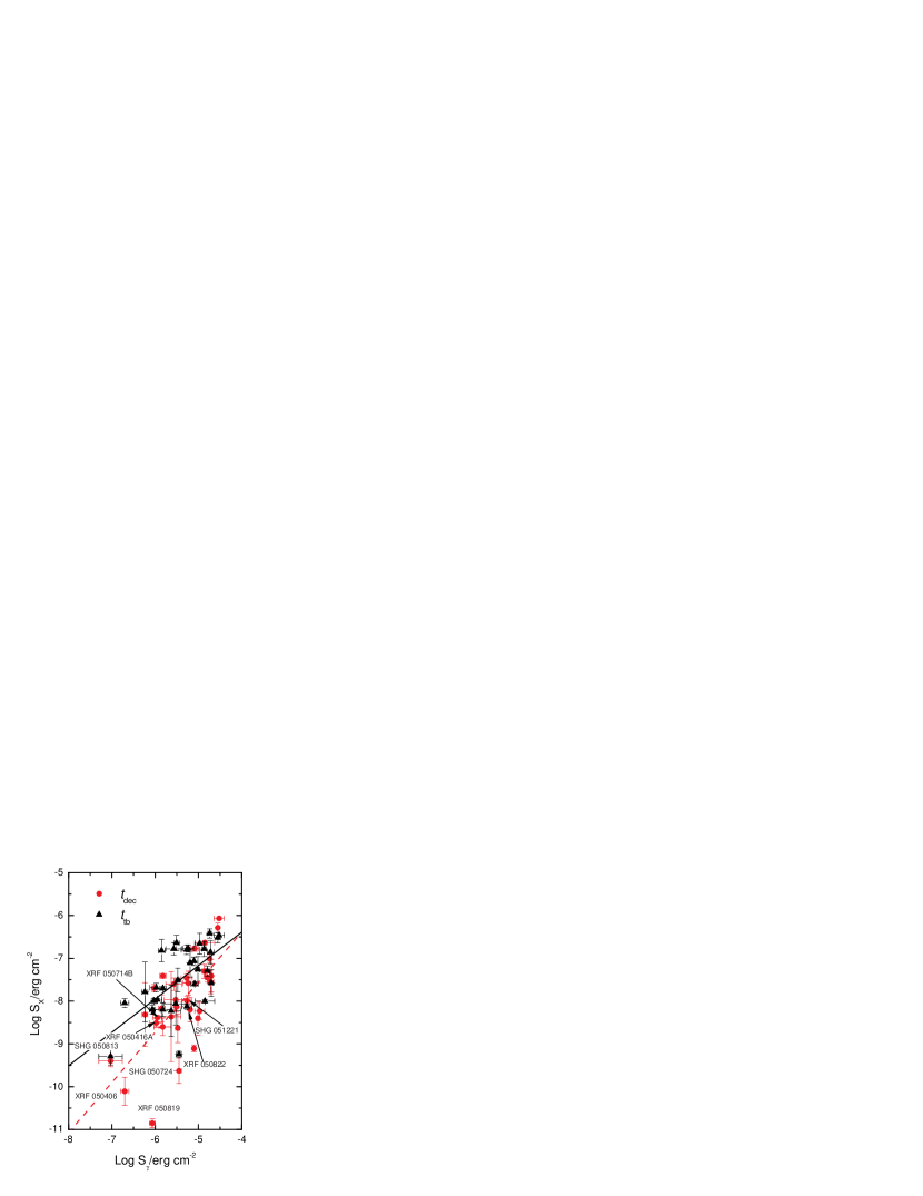
Figure 5: The extrapolated prompt emission fluence $S_{\gamma}$ against the X-ray fluence at $t_{\rm dec}$ (dots) and at $t_{b}$ (triangles). The solid and dashed lines, with slopes of 0.78 and 1.17, are the best fit to the data at $t_{b}$ and $t_{dec}$, respectively. The short-hard GRBs (SHGs) and X-ray flashes (XRFs) are marked.

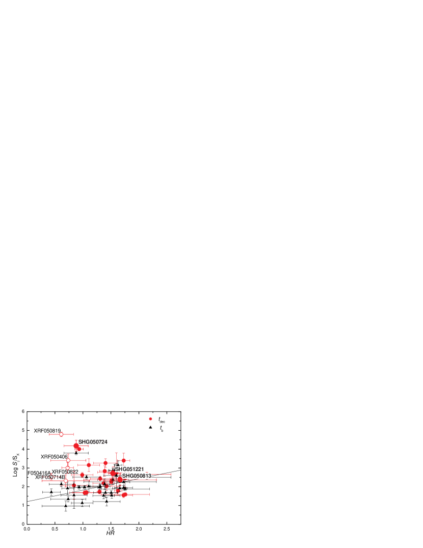
Figure 6: Ratios of $S_{\gamma}/S_{X}$ against the hardness ratio $HR$. The circles represent the data at $t_{dec}$, and the triangles represent the data at $t_{b}$. The short-hard GRBs (larger solid circles) and the XRFs (open circles) at $t_{dec}$ are marked. The straight line is the best fit of the data at $t_{b}$, which shows a shallow correction between the two quantities, with a linear correlation coefficient 0.61 and a chance probability $<0.01$.

4 GRB efficiency

4.1 Theoretical Models

In this section we explicitly derive the radiative efficiency for the GRBs in our sample according to eq.(1). The isotropic prompt emission energy $E_{\gamma}$ is derived from the extrapolated 1-10000 keV band fluence ($S_{\gamma}$) according to

$$E_{\gamma} = {4\pi D_{L}^{2}}S_{\gamma}{(1+z)^{-1}}$$ (3)

$$= 1.3\times 10^{51}~{}{\rm erg}~{}D_{L,28}^{2}(1+z)^{-1}S_{\gamma,-6}$$

where $D_{L}$ is the luminosity distance.

The derivation of $E_{K}$ requires detailed afterglow modeling. Regardless of whether there is indeed a long-lasting central engine, the energy injection process could be mimicked by introducing an “effective” long lasting central engine with luminosity $L=L_{0}(t/t_{0})^{-q}$. For the varying Lorentz factor injection model the Lorentz factor index $s$ could be related to an effective $q$ through $q=(10-2s)/(7+s)$ for an ISM medium and $q=4/(3+s)$ for a wind medium (Zhang et al. 2006). The injection then results in an evolving kinetic energy $E_{K}\propto t^{(1-q)}$. After the energy injection is over, the fireball can be described by the standard afterglow model. At any epoch during the injection phase, the afterglow emission level could be calculated by taking the kinetic energy at that time. So in our treatment, we still use the standard afterglow model to derive various parameters as functions of $E_{K}$, bearing in mind that $E_{K}$ may be time-dependent.

For a constant density medium, the typical synchrotron emission frequency, the cooling frequency and the peak spectral flux read (Sari et al. 1998; coefficients taken from Yost et al. 2003)

$$\nu_{m} = 3.3\times 10^{12}{\rm\ Hz}\left(\frac{p-2}{p-1}\right)^{2}(1+z)^{1/2}\epsilon_{B,-2}^{1/2}\epsilon_{e,-1}^{2}E_{K,52}^{1/2}t_{d}^{-3/2}$$ (4)

$$\nu_{c} = 6.3\times 10^{15}{\rm\ Hz}(1+z)^{-1/2}(1+Y)^{-2}\epsilon_{B,-2}^{-3/2}E_{K,52}^{-1/2}n^{-1}t_{d}^{-1/2}$$ (5)

$$F_{\nu,\max} = 1.6{\rm\ mJy}(1+z)D^{-2}_{28}\epsilon_{B,-2}^{1/2}E_{K,52}n^{1/2}~{}.$$ (6)

Here $t_{d}$ is the observer’s time in unit of days,

$$Y=[-1+(1+4\eta_{1}\eta_{2}\epsilon_{e}/\epsilon_{B})^{1/2}]/2$$ (7)

is the IC parameter, where $\eta_{1}={\rm min}[1,(\nu_{c}/\nu_{m})^{(2-p)/2}]$ (Sari & Esin 2001), and $\eta_{2}\leq 1$ is a correction factor introduced by the Klein-Nishina correction. The latter effect was treated in detail by Fan & Piran (2006). Here we adopt an alternative, approximate treatment. For the electron Lorentz factor $\gamma_{e,X}$ corresponding to the X-ray band emission, the synchrotron self-IC effect is significantly suppressed in the Klein-Nishina regime for the photons with energy $\nu>\nu_{\rm KN}$, where

$$\nu_{\rm KN} = h^{-1}\Gamma m_{e}c^{2}\gamma_{e,X}^{-1}(1+z)^{-1}$$ (8)

$$\simeq 2.4\times 10^{15}~{}{\rm Hz}~{}(1+z)^{-3/4}E_{52}^{1/4}\epsilon_{B,-2}^{1/4}t_{d}^{-3/4}\nu_{18}^{-1/2}~{},$$

and $h$ is the Planck’s constant. Based on the $\nu F_{\nu}$ spectrum of the standard synchrotron emission model (Sari et al. 1998), one can roughly estimate $\eta_{2}={\rm min}[1,(\nu_{\rm KN}/\nu_{c})^{(3-p)/2}]$ for slow cooling ($\nu_{m}<\nu_{c}$) and $\eta_{2}={\rm min}[1,(\nu_{\rm KN}/\nu_{m})^{1/2}]$ for fast cooling ($\nu_{c}<\nu_{m}$), where the factors $(\nu_{\rm KN}/\nu_{c})^{(3-p)/2}$ and $(\nu_{\rm KN}/\nu_{m})^{1/2}$ denote the fractions of the photon energy density that contributes to self-IC in the X-ray band in the slow and fast cooling regimes, respectively.

In previous analyses (e.g. Freedman & Waxman 2001; Berger et al. 2003; Lloyd-Ronning & Zhang 2004), the IC cooling was usually not taken into account. The inclusion of IC cooling modifies the X-ray afterglow light curves considerably (e.g. Wu et al. 2005), which also influences the derived GRB efficiency $\eta_{\gamma}$. Here we generally include the IC factor [power of $(1+Y)$] in the treatment (see also Fan & Piran 2006). The results are reduced to the previous pure synchrotron-dominated case when $Y\ll 1$.

For about 2/3 cases in our sample (22 out of 31), the X-ray band temporal decay index and the spectral index are consistent with the spectral regime $\nu>{\rm max}(\nu_{m},\nu_{c})$. This is the regime where $E_{K}$ is independent of $n$ and only weakly depends on $\epsilon_{B}$ and $p$, and therefore an ideal regime to measure $E_{K}$. One can derive the X-ray band energy flux as

$$\nu F_{\nu}(\nu=10^{18}~{}{\rm Hz}) = F_{\nu,\max}\nu_{c}^{1/2}\nu_{m}^{(p-1)/2}\nu_{X}^{(2-p)/2}$$ (9)

$$= 5.2\times 10^{-14}~{}{\rm ergs~{}s^{-1}~{}cm^{-2}}D_{28}^{-2}(1+z)^{(p+2)/4}$$

$$\times (1+Y)^{-1}f_{p}\epsilon_{B,-2}^{(p-2)/4}\epsilon_{e,-1}^{p-1}E_{K,52}^{(p+2)/4}t_{d}^{(2-3p)/4}\nu_{18}{{}^{(2-p)/2}}~{},$$

where

$$f_{p}=6.73\left(\frac{p-2}{p-1}\right)^{(p-1)}(3.3\times 10^{-6})^{(p-2.3)/2}$$ (10)

is a function of $p$, which is calculated in Figure 7. It peaks at $\sim 1.72$ when $p\sim 2.12$, and declines monotonically at large $p$ values. For example, at $p\sim 3$, $f_{p}$ is only $\sim 0.02$. This gives a nearly 2 orders of magnitude variation for $p=(2.01-3)$, and thus demands more careful treatments of individual bursts presumably having quite different $p$ values.

With eq.(9), one can derive $E_{K}$ at any time $t_{d}$ as

$$E_{K,52} = \left[\frac{\nu F_{\nu}(\nu=10^{18}~{}{\rm Hz})}{5.2\times 10^{-14}~{}{\rm ergs~{}s^{-1}~{}cm^{-2}}}\right]^{4/(p+2)}D_{28}^{8/(p+2)}(1+z)^{-1}t_{d}^{(3p-2)/(p+2)}$$ (11)

$$\times (1+Y)^{4/(p+2)}f_{p}^{-4/(p+2)}\epsilon_{B,-2}^{(2-p)/(p+2)}\epsilon_{e,-1}^{4(1-p)/(p+2)}\nu_{18}{{}^{2(p-2)/(p+2)}}$$

This could be reduced to $E_{K}\sim\epsilon_{e}^{-1}S_{X}D_{L}^{2}/(1+z)$ for $p\sim 2$. Comparing with eq.(3), we can see that as far as the efficiency problem is concerned the redshift-dependence is very weak.

Figure 7: The function $f_{p}$.

For nearly 1/3 cases in our sample (9 out of 31), the X-ray data are not consistent with being in the regime $\nu_{X}>{\rm max}(\nu_{m},\nu_{c})$ (which requires $\alpha=(3\beta-1)/2$ for the $F_{\nu}\propto t^{-\alpha}\nu^{-\beta}$ convention). The temporal decay slope in the normal decay phase is close to -1. This rules out the fast cooling case $\nu_{c}<\nu_{X}<\nu_{m}$ for both ISM and wind models. For slow cooling models ($\nu_{m}<\nu_{X}<\nu_{c}$), the temporal decay index derived from the wind model [$\alpha=(3\beta+1)/2$ for the $F_{\nu}\propto t^{-\alpha}\nu^{-\beta}$ convention, Chevalier & Li (2000)] is too steep compared with the data in our sample. One is then left with the only possibility, $\nu_{m}<\nu_{X}<\nu_{c}$ in the ISM model. In fact the observed $\alpha$ and $\beta$ are consistent with being in this regime [$\alpha=(3/2)\beta$]. The derived X-ray band energy flux is then

$$\nu F_{\nu}(\nu=10^{18}~{}{\rm Hz}) = F_{\nu,\max}(\nu_{m}/\nu_{X})^{(p-1)/2}$$ (12)

$$= 6.5\times 10^{-13}~{}{\rm ergs~{}s^{-1}~{}cm^{-2}}D_{28}^{-2}(1+z)^{(p+3)/4}$$

$$\times f_{p}\epsilon_{B,-2}^{(p+1)/4}\epsilon_{e,-1}^{p-1}E_{K,52}^{(p+3)/4}n^{1/2}t_{d}^{(3-3p)/4}\nu_{18}{{}^{(3-p)/2}}~{},$$

This gives

$$E_{K,52} = \left[\frac{\nu F_{\nu}(\nu=10^{18}~{}{\rm Hz})}{6.5\times 10^{-13}~{}{\rm ergs~{}s^{-1}~{}cm^{-2}}}\right]^{4/(p+3)}D_{28}^{8/(p+3)}(1+z)^{-1}t_{d}^{3(p-1)/(p+3)}$$ (13)

$$\times f_{p}^{-4/(p+3)}\epsilon_{B,-2}^{-(p+1)/(p+3)}\epsilon_{e,-1}^{4(1-p)/(p+3)}n^{-2/(p+3)}\nu_{18}{{}^{2(p-3)/(p+3)}}$$

Inspecting eq.(5), one can draw the conclusion that in order to have $\nu_{c}>\nu_{X}$ in the normal decay regime ($t_{d}\sim 1$), $\epsilon_{B}$ must be very small (e.g. $<(10^{-3}-10^{-4})$). Keeping a more or less constant $\epsilon_{e}\sim 0.1$, the $Y$ parameter (eq.[7]) does not increase significantly for a smaller $\epsilon_{B}$, since the $\eta_{2}$ parameter becomes much smaller due to the Klein-Nishina suppression. In order not to derive a unreasonably large $E_{K}$ value (limited by the total energy budget of the progenitor system), the data also require a small ambient density (e.g. $n<0.1$).

4.2 Calculation Results

Eqs. (11) and (13) suggest that the absolute value of $E_{K}$ depends on several unknown shock parameters. In order to calculate $\eta_{\gamma}$, the absolute value of $E_{K}$ is needed. This requires a detailed multi-wavelength study (e.g. Panaitescu & Kumar 2002; Yost et al. 2003) to constrain unknown shock parameters as well. Limited by the X-ray data alone, one inevitably needs to make some assumptions on the unknown shock parameters.

Our first step is to use the X-ray data (temporal index $\alpha_{X}$ and spectral index $\beta_{X}$) to determine the spectral regime the burst belongs to. In all the cases, we choose the “normal” decay phase for the temporal index ($\alpha_{2}$ for the broken power-law fit, or $\alpha_{1}$ for the single power-law fit if $\alpha_{1}$ is close to unity). This is because this segment has no contamination of energy injection (with unknown $q$ parameter). Using $\alpha_{X}$ and $\beta_{X}$ we check the spectral regime of the X-ray band by comparing the $\alpha-\beta$ relation of various models (e.g. Table 1 of Zhang & Mészáros 2004). We find that within the error uncertainties of the data, most bursts could be grouped into two spectral regimes: (I) $\nu_{X}>{\rm max}(\nu_{m},\nu_{c})$ (20 out of 31); and (II) $\nu_{m}<\nu_{X}<\nu_{c}$ in the ISM model (9 out of 31). Two bursts have unexpectedly large spectral indices, i.e. GRBs 050319 ($\beta_{X}=2.02\pm 0.47$) and 050714B ($\beta_{X}=4.50\pm 0.70$). The spectrum is likely dominated by the contribution of the GRB tail emission and we assume that in the afterglow phase they are in the regime of $\nu_{X}>{\rm max}(\nu_{m},\nu_{c})$, the default case. GRBs 050215B ($\beta_{X}\sim 0.5\pm 0.5$) and 050716 ($\beta_{X}=0.33\pm 0.03$) have very small spectral indices, and we assume that it is in the regime $\nu_{m}<\nu_{X}<\nu_{c}$. After determining the spectral regimes, we derive $p$ from $\beta_{X}$ ($\beta_{X}=-p/2$ for $\nu_{X}>{\rm max}(\nu_{m},\nu_{c})$ and $\beta_{X}=-(p-1)/2$ for $\nu_{m}<\nu_{X}<\nu_{c}$). Given the large error bars usually associated with the spectral indices, whenever $p\leq 2$ and $p>3$ we take $p=2.01$ and $p=3$, respectively.

4.2.1 $\nu_{X}>{\rm max}(\nu_{m},\nu_{c})$

Since there are too many unknown parameters for the regime II bursts (eq.[13]), we first ignore them and focus on the regime I bursts, whose $E_{K}$ essentially only depend on $\epsilon_{e}$. Previous broadband fitting suggests that $\epsilon_{e}$ is typically around 0.1 (Wijers & Galama 1999; Panaitescu & Kumar 2002; Yost et al. 2003; Liang et al. 2004; Wu et al. 2004). The value of $\epsilon_{B}$ has a large scatter for previous bursts but nonetheless has a typical value of $0.01$ (e.g. Panaitescu & Kumar 2002). The existence of regime II bursts suggest that at least some bursts have very small $\epsilon_{B}$. We therefore also consider the cases with a smaller $\epsilon_{B}$, say, $\sim 10^{-4}$. In any case $E_{K}$ is insensitive to $\epsilon_{B}$ in regime I.

Our calculation procedure for regime I GRBs is as follows.

1. Use the extrapolated $S_{\gamma}$ in the 1-10000 keV band to derive $E_{\gamma}$ according to eq.(3). Since $\eta_{\gamma}$ is insensitive to $z$, we take a moderate redshift, $z=2$, for those bursts whose redshifts are not directly measured.

2. Use $\beta_{X}$ and the 0.3-10 keV band flux to calculate the monochromatic flux at $10^{18}$ Hz, $F_{\nu}(\nu=10^{18}~{}{\rm Hz})$.

3. Calculate $E_{K,52}$ with eq.(11) at two epochs, $t_{\rm dec}$ and $t_{b}$. For each epoch we calculate two values: one value ($E_{K,52}^{(1)}$) for $(\epsilon_{e},\epsilon_{B})=(0.1,0.01)$, and another ($E_{K,52}^{(2)}$) for $(\epsilon_{e},\epsilon_{B})=(0.1,10^{-4})$. The $Y$ parameter is searched self-consistently according to the method described in §4.1.

4. Use eq.(1) to derive ${\eta}_{\gamma}^{(1)}$ and ${\eta}_{\gamma}^{(2)}$ at $t_{\rm dec}$ and $t_{b}$.

Table 3 displays our calculation results for regime I GRBs. Equation (11) indicates that the apparent dependence on $\epsilon_{B}$ is weak. This is strengthened by the Klein-Nishina effect since $Y$ does not increase significantly as $\epsilon_{B}$ is lowered. Comparing $E_{K}^{1}$ and $E_{K}^{2}$ (or $\eta_{\gamma}^{1}$ and $\eta_{\gamma}^{2}$) at a same epoch, we can see that the difference introduced by changing $\epsilon_{B}=0.01$ to $10^{-4}$ is not significant. In Fig.8 we show the $E_{K}$ contour in the $(\epsilon_{e},\epsilon_{B})$ plane for GRB 050219A. It again shows the result is insensitive to $\epsilon_{B}$, so that $\epsilon_{e}$ is the most sensitive parameter for determining $E_{K}$ and hence, for determining $\eta_{\gamma}$. The existence of the regime II bursts (which requires low values of $\epsilon_{B}$) suggests that if shock parameters are not too different from burst to burst, the $\epsilon_{B}$ value for the regime I bursts may be also low (e.g. the second parameter set, $(\epsilon_{e},\epsilon_{B})=(0.1,10^{-4})$, for the regime I calculations). This suggests slightly lower radiative efficiencies than previously estimated (typically taken as $\epsilon_{B}\sim 0.01$), since a lower $\epsilon_{B}$ nonetheless slightly increases $E_{K}$ despite a very shallow dependence.

Figure 8: Contours of $\log E_{K}$ in the $(\epsilon_{e},\epsilon_{B})$ plane for GRB 050219A.

Inspecting the calculated $\eta_{\gamma}$ for the bursts in the spectral regime I, we find that at $t_{\rm dec}$, 10 out of 22 bursts have a radiative efficiency $\eta_{\gamma}^{(1)}$ higher than $60\%$, sometimes even as high as $98\%$ (GRB 050819). The rest have much lower efficiencies, sometimes only a few percent. At $t_{b}$, on the other hand, the values of $\eta_{\gamma}$ are typically several percent or even lower. Those bursts with low efficiencies from the very beginning correspond to the cases without significant energy injection in the early phase. For illustration, in Fig.9 we present the combined BAT-XRT light curves in the XRT band for some GRBs having extremely high or low efficiencies at $t_{\rm dec}$ (see also O’Brien et al. 2006). It is evident that the XRT light curves of the high-$\eta_{\gamma}(t_{dec})$ GRBs have a very flat energy injection component and a prominent steeply decaying prompt emission tail (e.g. GRB 050315 and GRB 050714B). Those with low-$\eta_{\gamma}(t_{b})$, on the other hand, typically have a smooth transition from prompt emission to afterglow without a significant steep decay component and/or a shallow decay component due to energy injection (e.g. GRB 050401 and GRB 050712).

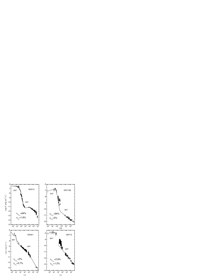
Figure 9: Comparisons of the joint-BAT-XRT light curves in the XRT band for some GRBs having extremely high or low efficiencies at $t_{dec}$.

In Fig.10 we plot $\eta_{\gamma}^{(1)}$ as a function of the hardness ratio $HR$. We again find that while there exists a shallow correlation between $\eta_{\gamma,t_{b}}^{(1)}$ and $HR$ (with index $1.12\pm 0.90$), such a correlation essentially disappears when $\eta_{\gamma}$ at $t_{\rm dec}$ is considered. This is consistent with the analysis in §2.2. The results suggest that if $E_{K}(t_{dec})$ is the relevant afterglow energy left over after the prompt emission, XRFs and GRBs intrinsically have similar radiative efficiencies, as opposed to the conclusion drawn using late-time X-ray data only.

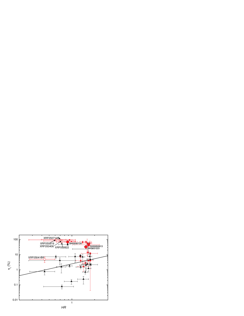
Figure 10: The radiative efficiency $\eta_{\gamma}^{(1)}$ against the hardness ratio $HR$. The circles represent the data at $t_{dec}$, and the triangles represent the data at $t_{b}$. The short-hard GRBs (larger solid circles) and the XRFs (open circles) at $t_{dec}$ are also marked. The dashed line is the best fit of the data at $t_{b}$, which shows a shallow correction between the two quantities similar to that shown in Figure 6.

Two short-hard GRBs 050724 and 050813 are in the spectral regime I. The results in Table 3 suggest that there is no noticeable difference between short, hard GRBs and long, soft GRBs as far as the radiative efficiencies are concerned. The same conclusion was drawn for the first short GRB with X-ray afterglow detection (GRB 050509b, Gehrels et al. 2005; Bloom et al. 2006), and is being verified by a larger sample of short GRBs in accumulation. To increase the short GRB sample, we have also performed the same analysis to GRB 051221A (e.g. A. Parsons et al. 2006, in preparation). The results are included in all the Tables and figures, making the total number of short bursts in our sample to 32. The inclusion of this burst strengthens the conclusion that short GRBs are no different from long GRBs in radiative efficiencies.

4.2.2 $\nu_{m}<\nu_{X}<\nu_{c}$

For the regime II bursts, we can set up an upper limit on $\epsilon_{B}$ using the light curves. Typically this limit is very low (say, $<10^{-4}$) since the afterglow light curves usually extend to very late epochs (say, $>1$ day). The efficiency estimated for these bursts have even larger uncertainties because $E_{K}$ depends on many unknown parameters, e.g. $\epsilon_{e}$, $\epsilon_{B}$, $n$, etc. Nonetheless, we perform some rough estimates with the following procedure.

To keep $\nu_{c}$ above $\nu_{X}$ for a long period of time (say, days), one must have a small $\epsilon_{B}$ and/or a small $n$. Sometimes one even needs to lower $\epsilon_{e}$ if one is reluctant to lower $n$. A lower $\epsilon_{B}$ and a lower $\epsilon_{e}$ would lead to a larger $E_{K}$ and hence, a lower $\eta_{\gamma}$. Since we do not know which parameter is in operation, we fix $\epsilon_{e}=0.1$ and $n=0.1$, and search $\epsilon_{B}$ downwards to find the highest $\epsilon_{B}$ that allows $\nu_{m}<\nu_{X}<\nu_{c}$ to be satisfied. In Table 4 we present our search results for the regime II bursts. The efficiency value listed does not represent the real value. There is no obvious reasons to argue why $\epsilon_{e}$ should be 0.1, why $n$ should be 0.1, or why $\epsilon_{B}$ is not even lower. Nonetheless, the value roughly indicates how $E_{K}$ and $\eta_{\gamma}$ look when the regime II spectral condition is satisfied. The results suggest that $\epsilon_{B}$ is rather low, in most cases lower than $10^{-4}$. The estimated $E_{K}$ is typically very high, and hence, the radiative efficiency is very low. This suggests that either these GRBs are intrinsically inefficient or the ambient densities of at least these GRBs are quite low, say $n\ll 0.1~{}{\rm cm}^{-3}$.

5 Conclusions and discussion

We present a detailed analysis on the prompt gamma-ray emission and the early X-ray afterglow emission for a sample of 31 GRBs detected by Swift and derived their radiative efficiencies. The sample includes both long and short GRBs and both normal GRBs and softer XRFs. This allows us to investigate how the GRB radiative efficiency vary globally within different populations. We summarize our findings in the following.

1. Due to the intrinsic limitation of the BAT instrument, it is very difficult to derive spectral parameters of the prompt emission and to extrapolate the BAT fluence to a broader band. We have developed a method by making use the hardness ratio information to derive spectral parameters assuming a Band function spectrum for all the bursts. This is probably the best effort with the available BAT data. The involved uncertainties is still large. It is also difficult to set errors to the quantities. The errors of $\Gamma_{1}$ and $\Gamma_{2}$ of the Band function are not accounted for in our analysis, but those of $E_{0}$ are included whenever possible. These errors are included to derive the errors of $S_{\gamma}$, which also include the uncertainties in the observations. Due to the intrinsic limitation of the method, the errors of $S_{\gamma}$ are likely under-estimated.

2. We compare our prompt emission data with those of BATSE (Preece et al. 2000) and HETE-2 (Lamb et al. 2005; Sakamoto et al. 2005) and generally find consistent results. Swift extends the fluence to the fainter regime and the hardness ratio to the softer regime with respect to BATSE. The derived properties of XRFs (including the 2:1 relative population between GRBs and XRFs) are generally consistent with those derived from the HETE-2 data.

3. The shallow decay component commonly detected in X-ray afterglows complicates the efficiency study. Previous analyses using late-time X-ray afterglow data (say, 10 hr) inevitably over-estimated $E_{K}$ and hence, under-estimated the GRB efficiency if the shallow decay is due to energy injection. We define two characteristic time epoches, the putative fireball deceleration time ($t_{\rm dec}$) and the epoch when the shallow decay is over ($t_{b}$), to study the efficiency problem. The efficiency derived at the former epoch [i.e. $\eta_{\gamma}(t_{dec})$] is likely the true efficiency for the models that interpret the shallow decay phase as due to energy injection (Zhang et al. 2006; Nousek et al. 2006; Panaitescu et al. 2006), while that derived at the later epoch [i.e. $\eta_{\gamma}(t_{b})$] is the true efficiency for some models that invoke precursor injection (Ioka et al. 2006) or delayed energy transition from the fireball to the circumburst medium (Kobayashi & Zhang 2006; Zhang & Kobayashi 2005).

4. We investigate both the observationally defined gamma-to-X fluence ratio ($R_{\gamma/X}$) and the theoretically defined efficiency ($\eta_{\gamma}$) at the two epochs. The former invokes direct observables and therefore is subject to less uncertainties. The later involve theoretical modeling, which depends on the uncertainties of many unknown microphysics parameters. The error of the latter is therefore difficult to quantify. Our approach is to fix model parameters, and only derive the errors introduced from the uncertainties of observations and data analyses. The errors of calculated efficiencies are therefore under-estimated. Nonetheless, some interesting features emerge from both the $R_{\gamma/X}$ analysis and the $\eta_{\gamma}$ analysis. At $t_{b}$, a shallow correlation between $R_{\gamma/X}$ or $\eta_{\gamma}$ and the hardness ratio is found. This is consistent with previous findings (Soderberg et al. 2004; Lloyd-Ronning & Zhang 2004; Lamb et al. 2005) that XRFs appear to be less efficient. However, the shallow correlation disappears when the analysis is performed at $t_{dec}$. This suggests that if the shallow decay is indeed due to energy injection, XRFs have similar radiative efficiencies as normal GRBs. The apparent low efficiency inferred using late time data must be attributed to some other reasons.

The result has important implications for understanding the nature of XRFs. In particular, it disfavors the model that interprets XRFs as events similar to GRBs but having smaller Lorentz factor contrasts and therefore lower radiative efficiencies (e.g. Barraud et al. 2005), if the shallow decay phase is due to energy injection. It suggests that XRFs are dim because the initial kinetic energy is also low, and that they gain larger kinetic energies later through energy injection. While there is no straightforward reason for energy injection in the radial direction (e.g. due to a long-lived central engine or pile-up of slow ejecta) for XRFs, some geometric models of XRFs indeed expect energy “injection” from the horizontal directions. These models, such as the quasi-universal Gaussian-like structured jet model (Zhang et al. 2004a; Dai & Zhang 2005; Yamazaki et al. 2004), invoke relativistic ejecta with variable luminosities and possibly variable Lorentz factors in a wide range of angles. While GRBs correspond to the cases when observers view the bright core component (e.g. the line of sight is inside the typical Gaussian angle), XRFs are those cases when observers view the off-axis jet at a larger viewing angle. As long as the bulk Lorentz factor of the ejecta is still relativistic in these directions, the prompt emission of XRFs is weaker (because of the low energy in the direction) but with a comparable efficiency as in the core direction, since the initial kinetic energy in the direction is also low. Later as the jet is decelerated, the observer in the off-axis direction would progressively receive the energy contribution from the energetic core so that the light curve shows an early shallow decay (e.g. Kumar & Granot 2003; Salmonson 2003). At later times, the effective kinetic energy in the viewing direction is enhanced, leading to an apparently high kinetic energy (and hence, an apparently low radiative efficiency). Such a picture might be consistent with the data. In fact, the long-term X-ray afterglow lightcurve of XRF 050416A could be modeled by such a model (Mangano et al. 2006).

Other geometric models of XRFs have been also discussed in the literature. The model involving sharp-edge jets viewed off beam (Yamazaki et al. 2002) predicts an initial rising light curve and a steep decay after reaching the peak due to sideways expansion, which is not favored by the data. Granot et al. (2005) suggested a smoother edge, which in effect is similar to the Gaussian jet model (Zhang et al. 2004a). The two-component jet model (Zhang et al. 2004b; Huang et al. 2004; Liang & Dai 2004; Peng et al. 2005) could be consistent with the data as long as the second component is not distinct enough to result in noticeable light curve features that are not detected. Power law structured jets (Zhang & Mészáros 2002b; Rossi et al. 2002) may also interpret XRFs (Jin & Wei 2004; D’Alessio et al. 2006), but the model predicts too large a XRF population (Lamb et al. 2005; Zhang et al. 2004a). Finally, the varying opening angle model for XRFs invoke very wide jets for XRFs (Lamb et al. 2005). However, there is no straightforward reason to expect the significant change of $E_{K}$ (and hence, $\eta_{\gamma}$) at early times in this model.

It is possible that the shallow decay phase is not due to energy injection. Numerical simulations (Kobayashi & Zhang 2006) suggest that the time scale for a fireball to transfer energy from the ejecta to the medium is long. It could be that the observed shallow decay phase reflects the epochs during which the energy transfer is going on. A Poynting-flux-dominated flow may further extend the energy transfer period further due to the inability of tapping kinetic energy of the shell with the presence of a reverse shock (Zhang & Kobayashi 2005). If this is the case, $E_{K}(t_{b})$ is the relevant kinetic energy to define GRB efficiency, and XRFs are then indeed intrinsically inefficient GRBs (e.g. Barraud et al. 2005). More detailed early data and modeling are needed to reveal whether such a possibility holds.

5. The absolute value of radiative efficiency is subject to the uncertainties of afterglow parameters. By inspecting the spectral index and the temporal decay index of the X-ray afterglows, we identify 22 bursts whose afterglow cooling frequency is below the X-ray band. In this regime the radiative efficiency is insensitive to parameters except for $\epsilon_{e}$. Assuming $\epsilon_{e}=0.1$, we find that $\eta_{\gamma}(t_{b})$ of most bursts are smaller than $10\%$, while $\eta_{\gamma}(t_{\rm dec})$ ranges from a few percents to $>90\%$. Some bursts have a low efficiency throughout, and they correspond to those bursts whose X-ray afterglow light curve smoothly join the prompt emission light curve without a distinct steep decay component or an extended shallow decay component.

The standard internal shock models predict that the GRB efficiency is only around $1\%$ (Kumar 1999; Panaitescu et al. 1999). Our results indicate that some GRBs satisfy such a constraint. On the other hand, a group of GRBs with an early shallow decay component challenge the internal shock model if $E_{K}(t_{\rm dec})$ is the relevant quantity to define the efficiency, as is required in most energy injection models. Suggestions have been made in the literature to increase the efficiency (e.g. Beloborodov 2000; Kobayashi & Sari 2001; Fan et al. 2004; Rees & Mészáros 2005; Pe’er et al. 2005). For those models that invoke $E_{K}(t_{b})$ to define the efficiency (e.g. Ioka et al. 2006; Kobayashi & Zhang 2006), the data are consistent with the expectation of the internal shock model. The typical efficiency in such a case is $10\%$ or lower.

6. The three short GRBs (050724, 050813 and 051221A) have similar efficiencies as long GRBs at both $t_{\rm dec}$ and $t_{b}$, despite their distinct progenitor systems (Gehrels et al. 2005; Fox et al. 2005; Villasenor et al. 2005; Hjorth et al. 2005; Barthelmy et al. 2005; Berger et al. 2005c; Bloom et al. 2006). Such a trend is being verified by more and more short GRB data, and will be reinforced by a larger sample of short GRBs in the future.

7. Although most of the X-ray afterglows in our sample are above the cooling frequency, 9 GRBs do have a cooling frequency higher than the X-ray band for a very long time, suggesting a very small $\epsilon_{B}$ and/or a low medium density $n\ll 0.1~{}{\rm cm}^{-3}$. An extremely low medium density may not be at odd for long GRBs. If some of these long GRBs explode in superbubbles created by precedented supernovae or GRBs, the ambient medium could reach such a low density.

Table 1: Prompt Gamma-Ray data for the GRBs in our sample

GRB	$T_{90}$	$\Gamma_{PL}$	$\chi^{2}$	$HR_{\rm obs}$	$\log S_{\gamma,obs}$	$\Gamma_{1}$	$\Gamma_{2}$	$E_{p}$	$\chi^{2}$	$\log S_{\gamma}$	$z^{ref.}$
	(s)				(erg s-1)			(keV)		(erg s-1)
GRB050126	30.0	-1.36${}_{-0.15}^{+0.15}$	1.20	1.60(.23)	-6.07(.04)	-1.00	-2.30	157${}^{+129.}_{-53.}$	1.19	-5.63(.23)	1.290
GRB050128	13.8	NaN		1.66(.14)	-5.29(.02)	-.71	-2.19	118${}^{+18.}_{-14.}$	0.87	-4.87(.05)
GRB050215B	10.4	-2.45${}^{+0.73}_{-1.02}$	0.84	.84(.23)	-6.63(.07)	-1.00	-2.45	$\sim$18	0.83	$\sim$-6.24
GRB050219A	23.0	NaN		1.73(.11)	-5.38(.02)	-.32	-2.30	102${}^{+8.}_{-8.}$	0.91	-5.01(.03)
GRB050315	96.0	-2.10${}_{-0.09}^{+0.09}$	0.87	.93(.08)	-5.49(.02)	-1.28	-2.20	37${}^{+8.}_{-8.}$	0.88	-5.10(.03)	1.950
GRB050319	15.0	-2.15${}_{-0.21}^{+0.20}$	0.83	.99(.19)	-5.91(.05)	-1.25	-2.15	$\sim$ 28	0.82	$\sim$-5.51	3.240
GRB050401	38.0	NaN		1.50(.11)	-5.07(.02)	-1.15	-2.65	132${}^{+16.}_{-16.}$	0.96	-4.74(.04)	2.900
GRB050406	5.0	-2.59${}^{+0.38}_{-0.45}$	1.23	.74(.32)	-7.09(.10)	-1.00	-2.59	$\sim$ 24	1.22	$\sim$-6.70
GRB050416A	5.4	-3.09${}^{+0.22}_{-0.24}$	0.93	.44(.16)	-6.37(.06)	-1.00	-3.22	$<15$	0.90	$\sim$-5.97	.654
GRB050422	60.0	-1.38${}_{-0.22}^{+0.22}$	0.98	1.54(.28)	-6.21(.05)	-.90	-2.30	123${}^{+99.}_{-42.}$	0.79	-5.83(.20)
GRB050502B	17.5	-1.65${}^{+0.14}_{-0.15}$	1.02	1.31(.18)	-6.33(.04)	-1.30	-2.30	102${}^{+85.}_{-36.}$	1.03	-5.95(.10)
GRB050525	11.5	NaN		1.30(.03)	-4.81(.01)	-1.01	-2.72	80${}^{+3.}_{-3.}$	0.41	-4.55(.01)	.606
GRB050607	26.5	-1.20${}_{-0.07}^{+0.07}$	0.98	1.75(.16)	-6.22(.04)	-1.04	-2.00	393${}^{+368.}_{-132.}$	0.99	-5.52(.27)
GRB050712	48.0	-1.48${}_{-0.18}^{+0.18}$	0.99	1.42(.24)	-5.96(.05)	-1.00	-2.30	126${}^{+103.}_{-44.}$	1.02	-5.57(.18)
GRB050713A	70.0	NaN		1.39(.09)	-5.28(.02)	-1.12	-2.30	312${}^{+50.}_{-50.}$	1.22	-4.72(.08)
GRB050713B	75.0	-1.53${}_{-0.17}^{+0.17}$	0.83	1.40(.22)	-5.34(.04)	-1.00	-2.30	109${}^{+59.}_{-32.}$	0.83	-4.97(.11)
GRB050714B	87.0	-2.59${}^{+0.32}_{-0.37}$	0.88	.69(.43)	-6.24(.08)	-1.00	-2.59	$\sim$20	0.86	$\sim$ -5.85
GRB050716	69.0	NaN		1.57(.10)	-5.20(.02)	-.87	-2.00	119${}^{+19.}_{-16.}$	0.88	-4.70(.04)
GRB050717	70.0	NaN		1.63(.07)	-5.84(.03)	-1.12	-2.30	1890${}^{+1600.}_{-760.}$	0.78	-4.85(.22)
GRB050721	39.0	-1.87${}^{+0.16}_{-0.17}$	1.04	1.06(.25)	-5.51(.06)	-1.12	-2.05	45${}^{+23.}_{-35.}$	1.04	-5.08(.09)
GRB050724	3.0	-2.11${}^{+0.24}_{-0.26}$	0.84	.88(.22)	-5.93(.06)	-0.65	-2.11	$\sim$25	0.83	$\sim$-5.45	.258
GRB050726	30.0	-0.99${}^{+0.21}_{-0.20}$	1.23	2.14(.43)	-5.70(.05)	-1.00	-2.30	$>$984	1.20	$>$-4.79
GRB050801	20.0	-1.95${}^{+0.19}_{-0.20}$	1.16	1.03(.27)	-6.51(.07)	-1.40	-2.00	$\sim 33$	1.14	$\sim$-6.02
GRB050802	20.0	-1.54${}_{-0.14}^{+0.14}$	0.93	1.37(.19)	-5.66(.04)	-1.12	-2.30	118${}^{+77.}_{-40.}$	0.95	-5.27(.13)	1.710
GRB050803	150.0	-1.43${}_{-0.11}^{+0.11}$	0.97	1.51(.15)	-5.65(.03)	-1.05	-2.30	150${}^{+68.}_{-38.}$	0.97	-5.24(.12)
GRB050813	.6	-1.42${}_{-0.39}^{+0.39}$	1.35	1.66(.65)	-7.37(.11)	-.40	-2.30	86${}^{+101.}_{-59.}$	1.29	-7.03(.27)
GRB050814	65.0	-1.85${}_{-0.18}^{+0.18}$	1.09	1.10(.20)	-5.74(.05)	-1.23	-2.77	58${}^{+28.}_{-16.}$	1.05	-5.48(.05)
GRB050819	40.0	-2.64${}^{+0.29}_{-0.32}$	0.99	.61(.22)	-6.45(.07)	-1.00	-2.64	$<$15	1.04	$<$-6.06(.07)
GRB050820A	270.0	-1.24${}_{-0.17}^{+0.17}$	1.26	1.73(.16)	-5.08(.02)	-1.00	-2.25	284${}^{+82.}_{-55.}$	1.27	-4.52(.12)	2.612
GRB050822	102.0	-2.48${}_{-0.15}^{+0.15}$	0.97	.73(.10)	-5.58(.03)	-1.00	-2.48	$\sim 36$	0.96	$\sim$ -5.19
GRB050826	45.0	-1.12${}^{+0.29}_{-0.28}$	0.81	1.76(.43)	-6.35(.07)	-.93	-2.30	$>240$	0.81	$>$-5.82
GRB051221A	1.4	NaN		1.53(.08)	-5.94(.01)	-1.08	-2.30	402${}^{+93.}_{-72.}$	1.06	-5.27(.11)	.547

Redshift references: (z1)Berger et al. (2005a), (z2) Berger et al. (2005b), (z3)Fynbo et al. (2005a), (z4)Fynbo et al. (2005b), (z5)Cenko et al. (2005), (z6)Foley et al. (2005), (z7)Berger et al. (2005c), (z8)Fynbo et al. (2005c), (z9)Ledoux et al. (2005), (z10) Berger & Soderberg (2005).

Table 2: Observations and Fitting Results of X-ray Afterglows

GRB	$\beta$	$\alpha_{1}$	$\alpha_{2}$	$\log(t_{b}/s)$	$\log S_{x,t_{\rm dec}}$	$\log S_{x,{t_{b}}}$	$\log S_{x,1h}$	$\log S_{x,10h}$
GRB050126	1.59( .38)	.95( .27)	–	–	-8.37(1.05)	-8.23( .60)	-8.27( .69)	-8.22( .59)
GRB050128	.85( .12)	.65( .10)	1.25( .10)	3.36( .10)	-7.30( .16)	-6.78( .18)	-6.79( .19)	-7.02( .23)
GRB050215B	.51( .50)	.82( .08)	–	–	-8.31( .75)	-7.79( .70)	-7.98( .71)	-7.80( .70)
GRB050219A	1.02( .20)	.59( .08)	–	–	-8.40( .40)	-7.26( .30)	-7.64( .32)	-7.23( .30)
GRB050315	1.50( .40)	.01( .09)	.74( .05)	4.10( .14)	-9.11( .08)	-7.07( .10)	-7.55( .08)	-6.89( .13)
GRB050319	2.02( .47)	.52( .03)	1.77( .19)	4.94( .13)	-8.14( .12)	-6.64( .18)	-7.24( .12)	-6.76( .12)
GRB050401	.98( .05)	.68( .05)	1.35( .05)	3.74( .04)	-7.01( .10)	-6.42( .11)	-6.44( .11)	-6.65( .12)
GRB050406	1.37( .25)	.51( .10)	–	–	-10.11( .33)	-8.05( .11)	-9.20( .14)	-8.71( .06)
GRB050416A	.80( .29)	.40( .05)	.95( .05)	3.18( .03)	-8.51( .10)	-7.68( .10)	-7.61( .10)	-7.55( .12)
GRB050422	2.23(1.09)	.86( .04)	–	–	-8.60( .20)	-8.20( .16)	-8.35( .17)	-8.21( .16)
GRB050502B	.81( .28)	.86( .01)	–	–	-8.38( .04)	-7.97( .03)	-8.12( .03)	-7.98( .03)
GRB050525	1.07( .02)	1.10( .05)	1.45( .05)	3.44( .05)	-6.29( .11)	-6.52( .12)	-6.56( .12)	-6.96( .13)
GRB050607	.77( .48)	1.01( .05)	2.46(1.65)	5.11( .24)	-7.97( .36)	-8.06( .49)	-7.99( .36)	-8.00( .36)
GRB050712	.90( .06)	.72( .01)	–	–	-7.86( .17)	-7.48( .14)	-7.62( .15)	-7.49( .14)
GRB050713A	1.30( .07)	.65( .10)	1.15( .10)	4.00( .04)	-7.55( .27)	-6.86( .27)	-6.96( .27)	-6.89( .28)
GRB050713B	.70( .11)	.30( .11)	.97( .07)	4.21( .23)	-8.23( .20)	-6.66( .24)	-7.06( .20)	-6.59( .29)
GRB050714B	4.50( .70)	.50( .06)	–	–	-8.17( .32)	-6.82( .26)	-7.36( .27)	-6.86( .26)
GRB050716	.33( .03)	1.06( .07)	–	–	-7.41( .38)	-7.58( .31)	-7.51( .32)	-7.57( .31)
GRB050717	1.15( .10)	1.49( .01)	–	–	-6.63( .05)	-8.00( .04)	-7.47( .04)	-7.96( .04)
GRB050721	.74( .15)	1.28( .01)	–	–	-6.78( .06)	-7.60( .05)	-7.30( .05)	-7.58( .05)
GRB050724	.95( .07)	.90( .0.1)	–	–	-9.21( .33)	-7.86( .07)	-8.56( .14)	-8.21( .06)
GRB050726	.94( .07)	.91( .10)	2.45( .10)	4.06( .04)	-7.45( .11)	-7.30( .12)	-7.28( .11)	-7.96( .14)
GRB050801	.72( .54)	1.10( .02)	–	–	-7.70( .09)	-7.99( .06)	-7.89( .07)	-7.99( .06)
GRB050802	.91( .19)	.65( .10)	1.65( .10)	3.76( .04)	-7.46( .10)	-6.80( .11)	-6.82( .10)	-7.26( .14)
GRB050803	.71( .16)	.61( .10)	–	–	-7.58( .28)	-6.77( .08)	-7.04( .14)	-6.65( .06)
GRB050813	2.42( .89)	.70( .10)	2.12( .10)	2.26( .12)	-9.40( .13)	-9.29( .20)	-10.69( .30)	-11.81( .36)
GRB050814	1.08( .08)	.62( .06)	–	–	-8.63( .34)	-7.51( .28)	-7.97( .29)	-7.59( .28)
GRB050819	1.18( .23)	-.06( .06)	.65( .10)	4.26( .16)	-10.85( .10)	-8.20( .11)	-8.89( .10)	-8.04( .14)
GRB050820A	.87( .09)	1.18( .01)	–	–	-6.07( .03)	-6.46( .01)	-6.27( .02)	-6.45( .01)
GRB050822	1.60( .06)	.46( .11)	.95( .04)	4.14( .31)	-8.20( .29)	-7.11( .33)	-7.37( .29)	-7.03( .38)
GRB050826	1.27( .47)	1.10( .01)	–	–	-7.41( .05)	-7.70( .04)	-7.60( .05)	-7.70( .04)
GRB051221A	1.04( .20)	1.07( .03)	–	–	-7.99( .11)	-8.13( .06)	-8.12( .06)	-8.19( .05)

Table 3: The derived kinetic energies and gamma-ray Efficiencies at $t_{dec}$ and $t_{b}$ for the GRBs in the spectral regime $\nu_{X}>\max(\nu_{m},\nu_{c})$ by assuming $(\epsilon_{e},\epsilon_{B})=(0.1,0.01)^{(1)}$ and $(\epsilon_{e},\epsilon_{B})=(0.1,0.0001)^{(2)}$

GRB	$\log E_{K}^{(1)}(t_{\rm dec})$	$\eta_{\gamma}^{(1)}(t_{\rm dec})$∗	$\log E_{K}^{(1)}(t_{b})$	$\eta_{\gamma}^{(1)}(t_{b})$∗	$\log E_{K}^{(2)}(t_{\rm dec})$	$\eta_{\gamma}^{(2)}(t_{\rm dec})$∗	$\log E_{K}^{(2)}(t_{b})$	$\eta_{\gamma}^{(2)}(t_{b})$∗
	(erg)	(100%)	(erg)	(100%)	(erg)	(100%)	(erg)	(100%)
GRB050126	51.86(.84)	57.78(48.81)	53.60(.48)	2.39( 2.84)	52.26(.84)	35.27(45.68)	54.00(.48)	.97(1.16)
GRB050128	54.48(.16)	4.03(1.51)	55.01(.17)	1.22(.50)	54.49(.16)	3.99(1.49)	55.02(.17)	1.21(.50)
GRB050219A	52.84(.39)	57.21(22.20)	54.05(.30)	7.57( 4.85)	52.85(.39)	56.09(22.33)	54.07(.30)	7.25(4.66)
GRB050315	51.69(.06)	93.55(.96)	54.59(.08)	1.79(.33)	52.09(.06)	85.24( 2.00)	54.99(.08)	.72(.13)
GRB050319	52.45(.10)	$\sim$ 70	55.59(.14)	$\sim 0.2$	52.85(.10)	$\sim$48	55.99(.14)	$\sim$.1
GRB050401	55.05(.10)	2.79(.70)	55.66(.11)	.70(.19)	55.06(.10)	2.76(.69)	55.66(.11)	.70(.18)
GRB050406	50.67(.28)	$\sim$80	54.38(.09)	$\sim$0.1	50.99(.28)	$\sim$66	54.69(.09)	$\sim$.04
GRB050416A	52.34(.10)	$\sim$5	53.18(.10)	$\sim$.8	52.35(.10)	$\sim$5	53.18(.10)	$\sim$0.8
GRB050422	51.80(.16)	68.99(12.56)	53.83(.13)	2.01( 1.06)	52.20(.16)	46.97(14.62)	54.23(.13)	.81(.43)
GRB050502B	53.40(.04)	3.99(.99)	53.84(.03)	1.51(.37)	53.41(.04)	3.95(.98)	53.84(.03)	1.50(.37)
GRB050525	53.50(.11)	7.64(1.78)	53.45(.11)	8.49(2.03)	53.56(.11)	6.61( 1.55)	53.52(.11)	7.36( 1.78)
GRB050607	53.82(.36)	4.11(4.06)	53.75(.49)	4.78(5.86)	53.82(.36)	4.06( 4.02)	53.75(.49)	4.72( 5.80)
GRB050712	54.18(.14)	1.63(.86)	55.03(.14)	.24(.13)	54.19(.14)	1.61(.85)	55.03(.14)	.23(.12)
GRB050713A	52.92(.24)	68.02(12.41)	54.37(.24)	7.07(3.76)	53.19(.24)	53.84(14.18)	54.63(.24)	4.00( 2.20)
GRB050714B	50.80(.25)	$\sim$96	53.49(.21)	$\sim 4$	51.20(.25)	$\sim 89$	53.89(.21)	$\sim 2$
GRB050717	53.91(.05)	14.11( 6.38)	53.22(.04)	44.47(12.90)	54.05(.05)	10.65(5.01)	53.36(.04)	36.74(12.14)
GRB050724	50.40(.29)	69.23(14.68)	50.81(.07)	46.54(5.16)	50.40(.29)	68.98(14.75)	50.81(.07)	46.26(5.15)
GRB050813	51.03(.10)	44.81(16.69)	51.45(.16)	23.63(13.13)	51.43(.10)	24.43(12.46)	51.85(.16)	10.96(7.10)
GRB050814	52.17(.32)	67.78(16.47)	53.59(.27)	7.38(4.31)	52.25(.32)	63.80(17.42)	53.67(.27)	6.26(3.70)
GRB050819	49.95(.09)	$\sim 99$	53.02(.10)	$\sim$7	50.11(.09)	$\sim$98.	53.18(.10)	$\sim 5$
GRB050822	52.43(.23)	$\sim$69	54.59(.27)	$\sim$ 1.55(.94)	52.83(.23)	$\sim$47	54.99(.27)	$\sim.6$
GRB050826	53.01(.05)	$>12$	53.80(.04)	$>2$	53.25(.05)	$>7$	54.04(.04)	$>1$
GRB051221A	51.92(.11)	32.56( 7.83)	51.90(.06)	33.57(6.54)	51.96(.11)	30.61( 7.57)	51.94(.06)	31.59( 6.33)

^∗ The derived $\eta$ is insensitive to the redshift. For those bursts whose redshifts are not available we take $z=2$ in the calculation. The errors of $\eta$ are calculated by considering only the errors from the extrapolated gamma-ray fluences and the observed X-ray fluxes. Therefore, the errors of $\eta$ only reflect the observational errors. $E_{K}$ is sensitive to microphysics parameters that are poorly constrained. The true errors of $\eta$ should be significantly larger than what are reported here.

Table 4: Derived kinetic energies and gamma-ray efficiencies at $t_{dec}$ and $t_{b}$ for the GRBs in the spectral regime $\nu_{m}<\nu_{X}<\nu_{c}$ with $\epsilon_{e}=0.1$

GRB	$\epsilon_{B}$	$E_{K,52}(t_{\rm dec})$	$\eta_{\gamma}(t_{\rm dec})$	$E_{K,52}(t_{b})$	$\eta_{\gamma}(t_{b})$
		(erg)	(100%)	(erg)	(100%)
GRB050215B	$3\times 10^{-6}$	53.65( 1.49)	$\sim 1$	54.17( 1.40)	$\sim$0.4
GRB050713B	$4\times 10^{-6}$	52.01( .35)	90.68( 7.19)	54.98( .42)	1.03( 1.02)
GRB050716	$3\times 10^{-7}$	55.96( .76)	.20( .36)	55.09( .62)	1.48( 2.10)
GRB050721	$9\times 10^{-5}$	54.55( .10)	2.11( .66)	53.54( .08)	18.29( 4.35)
GRB050726	$5\times 10^{-5}$	53.22( .16)	$>$48	54.38( .18)	$>$6
GRB050801	$2\times 10^{-4}$	52.84( .15)	$\sim 11$	52.93( .10)	$\sim$9
GRB050802	$2\times 10^{-5}$	52.95( .16)	29.60( 9.72)	54.79( .17)	.61( .29)
GRB050803	$6\times 10^{-6}$	53.12( .48)	29.37( 23.78)	54.79( .14)	.88( .37)
GRB050820A	$7\times 10^{-7}$	56.50( .04)	.14( .04)	56.22( .02)	.27( .07)

References

- (1) Amati, L., et al. 2002, A&A, 390, 81
- (2) Band, D., et al. 1993, ApJ, 413, 281
- (3) Barthelmy, S. et al. 2005a, Nature, 438, 994
- (4) ——. 2005b, Space Sci. Rev. 120, 143
- (5) Barraud, C., Daigne, F., Mochkovitch, R., Atteia, J. L. 2005, A&A, 440, 809
- (6) Beloborodov, A. M. 2000, ApJ, 539, L25
- (7) Berger, E., Kulkarni, S. R. & Frail, D. A. 2003, ApJ, 590, 379
- (8) Berger, E. et al. 2005a, ApJ, 629, 328
- (9) Berger E., et al. 2005b, ApJ, 634, 501
- (10) Berger, E. et al. 2005c, Nature, 438, 988
- (11) Berger, E. & Soderberg, A. M. 2005, GCN 4384
- (12) Bloom, J. S. et al. 2006, ApJ, 638, 354
- (13) Burrows, D. N. et al. 2005a, Space Sci. Rev. 120, 165
- (14) Burrows, D. N. et al. 2005b, Science, 309, 1833
- (15) Cenko S. B. et al. 2005, GCN 3542
- (16) Chevalier, R. A.& Li, Z. Y. 2000, ApJ, 536, 195
- (17) Cui, X. H., Liang, E. W., Lu, R. J. 2005, ChJAA, 5, 151
- (18) Dai, X. & Zhang, B. 2005, ApJ, 621, 875
- (19) Dai, Z. G. 2004, ApJ, 606, 1000
- (20) Dai, Z. G. & Lu, T. 1998, A&A, 333, L87
- (21) Dai, Z. G., Wang, X. Y., Wu, X. F. & Zhang, B. 2006, Science, 311, 1127
- (22) Dermer, C. D, Chiang, J., Böttcher, M. 1999, ApJ, 513, 656
- (23) D’Alessio, V., Piro, L. & Rossi, E. M. 2006, A&A, in press (astro-ph/0511272)
- (24) Eichler, D. & Granot, J. 2006, ApJ, 641, L5
- (25) Fan, Y. Z. & Piran, T. 2006, MNRAS, 369, 197
- (26) Fan, Y. Z., & Wei, D. M. 2005, MNRAS, 364, L42
- (27) Fan, Y. Z., Wei, D. M., & Zhang, B. 2004, MNRAS, 354, 1031
- (28) Foley R. J. et al. 2005, GCN Circ. 3483, http://gcn.gsfc.nasa.gov/gcn/gcn3/3483.gcn3
- (29) Fox, D. B. et al. 2005, Nature, 437, 845
- (30) Frail, D. A., et al. 2001, ApJ, 562, L55
- (31) Freedman, D. L. & Waxman, E. 2001, ApJ, 547, 922
- (32) Fynbo, J. P. U., et al. 2005a, GCN Circ. 3136, http://gcn.gsfc.nasa.gov/gcn/gcn3/3136.gcn3
- (33) Fynbo,J. P. U., et al. 2005, GCN 3749
- (34) Fynbo, J. P. U., et al. 2005b, GCN Circ. 3176, http://gcn.gsfc.nasa.gov/gcn/gcn3/3176.gcn3
- (35) Gehrels, N. et al. 2004, ApJ, 611, 1005
- (36) Gehrels, N. et al. 2005, Nature, 437, 851
- (37) Ghirlanda, G., Celotti, A., Ghisellini, G. 2003, A&A, 406, 879
- (38) Granot, J., Konigl, A. & Piran, T. 2006, MNRAS, 370, 1946
- (39) Granot, J. & Kumar, P. 2006, MNRAS, 366, L13
- (40) Granot, J., Ramirez-Ruiz, E., & Perna, R. 2005, ApJ, 630, 1003
- (41) Golenetskii, S. et al. 2005a, GCN 3179
- (42) Golenetskii, S. et al. 2005b, GCN
- (43) Golenetskii, S. et al. 2005c, GCN
- (44) Golenetskii, S. et al. 2005d, GCN
- (45) Heise, J. et al. 2003, AIP Conf. Proc. 662, 229
- (46) Hjorth, J. et al. 2005, Nature, 437, 859
- (47) Huang, Y. F., Dai, Z. G., Lu, T. 2002, MNRAS, 332, 735
- (48) Huang, Y. F., Wu, X. F., Dai, Z. G., Ma, H. T. & Lu, T. 2004, ApJ, 605, 300
- (49) Hurley, K., Sari, R., & Djorgovski, S. G. 2002, astro-ph/0211620
- (50) Ioka, K., Kobayashi, S. & Zhang, B. 2005, ApJ, 631, 429
- (51) Ioka, K., Toma, K., Yamazaki, R. & Nakamura, T. 2006, A&A, in press (astro-ph/0511749)
- (52) Jin, Z.-P. & Wei, D.-M. 2004, ChJAA, 4, 473
- (53) King, A., O’Brien, P. T., Goad, M. R., Osborne, J., Olsson, E. & Page, K. 2005, ApJ, 630, L113
- (54) Kippen, M. et al. 2003, AIP Conf. Proc. 662, 244
- (55) Kobayashi, S., Piran, T., & Sari, R. 1999, ApJ, 513, 669
- (56) Kobayashi, S., Ryde, F. & MacFadyen, A. 2002, ApJ, 577, 302
- (57) Kobayashi, S. & Sari, R. 2001, ApJ, 551, 934
- (58) Kobayashi, S. & Zhang, B. 2006, ApJ, submitted (astro-ph/0608132)
- (59) Krimm, H. A. et al. 2006, ApJ, in press (astro-ph/0605507)
- (60) Kumar, P. 1999, ApJ, 532, L113
- (61) Kumar, P. & Granot, J. 2003, ApJ, 591, 1075
- (62) Kumar, P.& Panaitescu, A. 2000, ApJ, 541, L51
- (63) Kumar, P., & Piran, T. 2000, ApJ, 532, 286
- (64) Lamb, D. Q., Donaghy, T. Q. & Graziani, C. 2005, ApJ, 620, 355
- (65) Ledoux C. et al. 2005, GCN Circ. 3860
- (66) Liang, E. W. et al. 2006, ApJ, 646, 351
- (67) Liang, E. W., Dai, Z. G., Wu, X. F. 2004, ApJ, 606, L29
- (68) Liang, E. W., Dai, Z. G. 2004, ApJ, 608, L9
- (69) Lloyd, N. M., Petrosian, V. & Mallozzi, R. S. 2000, ApJ, 534, 227
- (70) Lloyd-Ronning, N. M. & Zhang, B. 2004, ApJ, 613, 477
- (71) Mangano, V. et al. 2006, ApJ, in press (astro-ph/0603738)
- (72) Mészáros, P. 2002, ARA&A, 40, 137
- (73) Mészáros, P., Ramirez-Ruiz, E., Rees, M. J. & Zhang, B. 2002, ApJ, 578, 812
- (74) Mészáros, P., & Rees, M. J. 1997, ApJ, 476, 232
- (75) Nousek, J. et al. 2006, ApJ, 642, 389
- (76) O’Brien, P. et al. 2006, ApJ, in press (astro-ph/0601125)
- (77) Panaitescu, A., & Kumar, P. 2001, ApJ, 560, L49
- (78) Panaitescu, A., Mészáros, P., & Rees, M. J. 1998, ApJ, 503, 314
- (79) Panaitescu, A., Mészáros, P., Gehrels, N., Burrows, D. & Nousek, J. 2006, MNRAS, 366, 1357
- (80) Panaitescu, A., Spada, M. & Mészáros, P. 1999, ApJ, 522, L105
- (81) Parson, A. et al. 2006, ApJ, to be submitted
- (82) Pe’er, A., Mészáros, P. & Rees, M. J. 2005, 635, 476
- (83) Peng, F., Königl, A. & Granot, J. 2005, ApJ, 626, 966
- (84) Perna, R., Armitage, P. J. & Zhang, B. 2006, ApJ, 636, L29
- (85) Piran, T. 1999, Phys. Rep. 314, 575
- (86) ——. 2005, Rev. Mod. Phys., 76, 1143
- (87) Preece, R. D., Briggs, M. S., Mallozzi, R. S., Pendleton, G. N., Paciesas, W. S., & Band, D. L. 2000, ApJS, 126, 19
- (88) Proga, D. & Zhang, B. 2006, MNRAS, 370, L61
- (89) Rees, M. J., & Mészáros, P. 1994, ApJ, 430, L93
- (90) ——. 1998, ApJ, 496, L1
- (91) ——. 2005, ApJ, 628, 847
- (92) Roming, P. W. A. et al., 2006, ApJ, in press (astro-ph/0509273)
- (93) Rossi, E., Lazzati, D. & Rees, M. J. 2002, MNRAS, 332, 945
- (94) Sakamoto, T. et al. 2005, ApJ, 629, 311
- (95) ——. 2006, ApJ, 636, L73
- (96) Salmonson, J. D. 2003, ApJ, 592, 1002
- (97) Sari, R. & Esin, A. A. 2001, ApJ, 548, 787
- (98) Sari, R., & Mészáros, P. 2000, ApJ, 535, L33
- (99) Sari, P., Piran, T. & Narayan, R. 1998, ApJ, 497, L17
- (100) Schady, P. et al. 2006, ApJ, 643, 276
- (101) Soderberg, A. et al. 2004, ApJ, 606, 994
- (102) ——. 2005, 627, 877
- (103) Tagliaferri, G. et al. 2005, Nature, 436, 985
- (104) Toma, K., Ioka, K., Yamazaki, R. & Nakamura, T. 2006, ApJ, 640, L139
- (105) Villasenor, J. S. et al. 2005, Nature, 437, 855 bibitem[]1280 Wijers, R. A. M. J.& Galama, T. J. 1999, ApJ, 523, 177
- (106) Wu, X. F., Dai, Z. G., Liang, E. W. 2004, ApJ, 615, 359
- (107) Wu, X. F., Dai, Z. G., Huang, Y. F., & Lu, T. 2005, ApJ, 619, 968
- (108) Wu, X. F., Dai, Z. G., Wang, X. Y., Huang, Y. F., Feng, L. L., Lu, T., 2006, ApJ, submitted (astro-ph/0512555)
- (109) Yamazaki, R., Ioka, K. & Nakamura, T. 2002, ApJ, 571, L31
- (110) Yamazaki, R., Ioka, K. & Nakamura, T. 2004, ApJ, 607, L103
- (111) Yost, S., Harrison, F. A., Sari, R., & Frail, D. A. 2003, ApJ, 597, 459
- (112) Zhang, B., Dai, X., Lloyd-Ronning, N. M. & Mészáros, P. 2004a, ApJ, 601, L119
- (113) Zhang, B., Fan, Y. Z., Dyks, J., Kobayashi, S., Mészáros, P., Burrows, D. N., Nousek, J. A. & Gehrels, N. 2006, ApJ, 642, 354
- (114) Zhang, B., & Kobayshi, S. 2005, ApJ, 628, 315
- (115) Zhang, B., & Mészáros, P. 2001, ApJ, 552, L35
- (116) ——. 2002a, ApJ, 566, 712
- (117) ——. 2002b, ApJ, 571, 876
- (118) ——. 2002c, ApJ, 581, 1236
- (119) ——. 2004, IJMPA, 19, 2385
- (120) Zhang, W., Woosley, S. E., & Heger, A. 2004b, ApJ, 608, 365