On The Size of Structures in the Solar Corona

Abstract

Fine-scale structure in the corona appears not to be well resolved by current imaging instruments. Assuming this to be true offers a simple geometric explanation for several current puzzles in coronal physics, including: the apparent uniform cross-section of bright threadlike structures in the corona; the low EUV contrast (long apparent scale height) between the top and bottom of active region loops; and the inconsistency between loop densities derived by spectral and photometric means. Treating coronal loops as a mixture of diffuse background and very dense, unresolved filamentary structures address these problems with a combination of high plasma density within the structures, which greatly increases the emissivity of the structures, and geometric effects that attenuate the apparent brightness of the feature at low altitudes. It also suggests a possible explanation for both the surprisingly high contrast of EUV coronal loops against the coronal background, and the uniform “typical” height of the bright portion of the corona (about 0.3 $R_{\odot}$) in full-disk EUV images. Some ramifications of this picture are discussed, including an estimate (10-100 km) of the fundamental scale of strong heating events in the corona.

1 Introduction

Since the introduction of EUV coronal imaging, bright coronal loops have been seen to have uniform thickness; several examples are illustrated in Figure 1. Because coronal bright structures are thought to be magnetically confined, this is a surprising result. Uniform-thickness flux bundles require constant magnetic field strength along the feature; this implies that tall, uniform-thickness bright structures in the corona must somehow be confined not only against gas pressure, but also against magnetic pressure. Much recent work has been devoted to understanding the physics of these structures, and several terms have been used to describe them. I suggest “thread” as a purely observational term to refer to thin, curvilinear features such as may be seen in the image plane of a solar instrument, avoiding any particular physical model for the corresponding coronal structure; phrases such as “filamentary structure”, “flux tube”, or “elementary structure”, which themselves carry some implicit meaning about the physics, may then be used to describe the structure in the corona itself. Furthermore, throughout this article I refer to objects in the image plane of a telescope as “features” and objects in the solar corona as “structures”.

Thin thread features are nearly always seen embedded in larger coronal features (for example active region loops) that expand with altitude as expected from force-free or potential field lines, but the smallest threads very clearly have uniform thickness in solar EUV images. Considerable effort has been put into understanding the physics of the corresponding solar structures. Aschwanden and Nitta (2000) pointed out that inhomogeneous structure can influence the ionization temperature gradient inferred via filter-ratio or differential emission-measure techniques applied to EUV image features. Comparison of TRACE-visible active region loops to simple hydrostatic atmospheric models shows that the tops of tall threaded loops seem overdense by a factor of up to 100 compared to hydrostatic solutions or, equivalently, that the threads have apparent intensity scale heights much longer than the calculated thermal scale height in the corona (e.g. Doyle et al. 1985; Aschwanden and Nitta 2000; Winebarger et al. 2003; Fuentes et al. 2006). Supporting a longer-than-thermal density scale height over such ranges requires extreme measures, such as ballistic siphon flows or wave pressure, that are not reflected in the spectral data. Simple calculation shows that doubling the density scale height of a 0.2 $R_{\odot}$ tall structure requires a basal speed of over 150 km sec^-1, compared to typical active region loop Doppler shifts of only 20-100 km sec^-1 as observed with SOHO/CDS (Fredvik et al. 2002). Taller structures or more uniform density profiles require even higher speeds for such support.

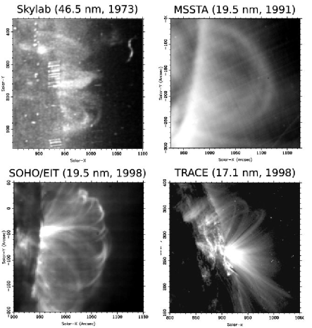
Figure 1: Limb images at the same spatial scale from four different UV imagers demonstrate the long-observed constant-width appearance of coronal loops. The apparent constant width varies from instrument to instrument. It is due to resolution effects in data from the Skylab “overlappograph” (Tousey et al. 1977; Feldman 1987) at ~8”, the Multi-Spectral Solar Telescope Array (Walker et al. 1991) at ~10”, and the Extreme-Ultraviolet Imaging Telescope (Delaboudiniere et al. (1995)) at 5”. I argue that the Transition Region and Coronal Explorer (Handy et al. 1998), the highest resolution existing EUV imager at ~1”, also does not resolve the filamentary structure within active regions.

The emission from some of these filamentary structures has been identified by Aschwanden and Nightingale (2005) as nearly thermally homogeneous, leading those authors to identify some particularly cleanly presented threads as “elementary” coronal structures having uniform cross-section versus position and a filling factor nea unity with constant temperature and density. Fuentes et al. (2006) have made detailed quantitative studies of threads’ profiles in a large sample of active regions . However, similar thin, bright active region loops yield much higher densities from density-sensitive line ratios than expected from photometric considerations (Warren and Winebarger 2003).

These inconsistencies all appear to be tied to a measurement that is not solid: the width of the structures themselves. The uniform thickness features seen in each panel of Figure 1 are close to the resolution limit of the corresponding telescope. In fact, TRACE, the highest resolution EUV telescope currently available, shows that active region loops appear composed of uniform-thickness threads about 1-2 Mm in width, which diverge one from the other as might be expected of individual field lines. One may conclude that the constant width of threads observed with earlier instruments was an instrumental effect: the underlying structures must have expanded with altitude as do complete bundles of threads in TRACE images. That conclusion, in turn, raises the question of whether constant-width features in the TRACE images are due to thin, variable width structures that are simply not well resolved.

Assuming that threaded loops observed with TRACE are not fully resolved eliminates two important problems. First, it avoids the theoretical problem of how to keep the structures confined compared to the surrounding general expansion, because if unresolved the structures do not have to be confined at all compared to a force-free field. In that case, they may expand laterally with altitude at the same relative rate as a force-free flux tube, provided only that each feature’s cross-section remains below or at least near the telescope resolution limit. Secondly, it provides a geometric explanation for the very long apparent scale height of active region loops seen with TRACE, rendering the measured intensity profiles consistent with hydrostatic equilibrium within each loop: if the size of the feature is permitted to vary with height, then geometrical considerations can provide sufficient extra brightness at high altitudes to explain the typical coronal intensity profiles, even if the loops are supported only hydrostatically.

Coronal loops are visible to surprisingly high altitudes with EUV imagers in general and TRACE in particular. It is not uncommon for an active region on the limb to be seen out to 140 Mm (0.2 $R_{\odot}$) or higher, and the “background corona” is visible out to about 0.3 $R_{\odot}$ in typical images from EIT Delaboudiniere et al. 1995. The scale height of 1-2 MK plasma near the solar surface is 50-100 Mm respectively (0.07 - 0.14 $R_{\odot}$), smaller than these typical EUV feature heights. If the plasma in the loops is in hydrostatic equilibrium, both the top and bottom of a uniform-thickness coronal structure as tall as 0.2-0.3 $R_{\odot}$ should not be readily visible in a linear scale image. However, if the thickness of the structure varies then the instrument images a different volume of plasma in a single pixel at different altitudes. Higher up, the tube should be both broader and thicker, and hence brighter, than would be expected for a uniform thickness flux tube. This effect is large enough to compensate for a hydrostatic density profile with altitude, out to (coincidentally) 0.2-0.3 $R_{\odot}$, after which the hydrostatic lapse rate dominates and the features rapidly dim. In turn, this provides a very clean explanation for the overall coronal morphology as seen with EUV imagers.

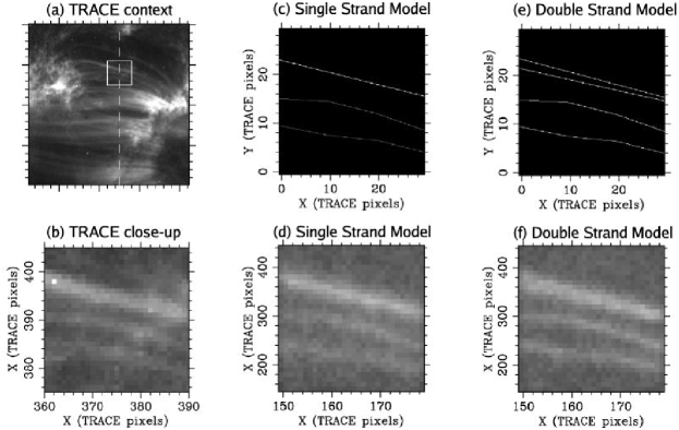
Figure 2: A simple forward model of threaded loops in an active region imaged by TRACE in the 171 Å passband on 1999 April 7 at 1:26 UT. (a) Context image of the active region. (b) Close-up of a small region of interest. (c) A simple model of “elementary” coronal structures (d) The model after convolution, pixelation, noise and pedestal were added. (e) A tapered dual-strand model of the top thread. (f) Dual-strand model after convolution, pixelation, noise, and pedestal. Neither of the two models is readily distinguished from the TRACE image.

In the following sections, I explore the hypothesis that elementary coronal features are not resolved and demonstrate that it is consistent with individual TRACE images and a hydrostatic corona. §2 is a discussion of telescope resolution, including a forward model of a simple structure close to the resolution limit of a telescope, and a demonstration of confusion effects in interpretation of solar data. §3 demonstrates that unresolved structure can greatly enhance the apparent scale height of bright features in the corona. §4 uses a forward model to reproduce the general appearance of active regions seen with TRACE using only geometry and hydrostatic density profiles. §5 is a study of the morphology of several threaded active regions observed with TRACE, including estimates of the size scale of unresolved features at the base of the active regions. All of these analyses are simple but sufficient to demonstrate a geometrical effect that has previously been ignored and that strongly affects interpretation of coronal EUV images. In §6, I conclude that unresolved loop structure is the simplest explanation for the observed intensity profile and apparent uniform thickness of active region loops observed with TRACE, discuss implications for the time evolution of active region threads, and call for higher resolution observations.

2 Telescope resolution

The TRACE telescope has a pixel size of 0.5 arc seconds (Handy et al. 1998) and a point-spread function with a full-width at half-maximum of about 2.25 pixels (e.g. Golub et al. 1999; Gburek, Sylwester, and Martens 2006). This is similar to the observed width of coronal threads in TRACE EUV images of active regions, weakening inferences that may be drawn from the image geometry about the size of the corresponding coronal structures on the Sun. Some authors (e.g. Fuentes et al. 2006) have taken great care in analyzing the size of active region filamentary structures based on observations of threads, but even such careful studies may have doubt shed on them by interaction between barely resolved structures, background noise, and other superposed features in the image plane. These effects can mimic those of a larger PSF, greatly weakening the commonly-held hypothesis that threads are adequately resolved in TRACE images (and hence that the size of solar filamentary structures may be determined from the image-plane size of the corresponding features).

To demonstrate the effects of random noise and telescope PSF on simple, compact linear structures, I implemented a simple 2-D forward model of the TRACE point-spread function to demonstrate the effects of noise and background structure on resolution of fine-scale loops. Figure 2 shows a simple treatment of three threads in an active region observed by TRACE. A small region-of-interest was modeled as three or four infinitely thin threads that were convolved with a circularly symmetric model PSF with a FWHM of 2.25 TRACE pixels; pixelated; and subjected to background pedestal and both uncorrelated (“photon”) and locally correlated (“solar background”) noise fields. I ran two forward models of the image: one with a single bright thread at the top and one with two less bright threads at distances of up to two TRACE pixels. The models were not distinguishable, indicating that structures with apparent size less than two TRACE pixels cannot be distinguished visually from structures of zero width. In either case, the resulting bright features had apparent visual widths of 5-6 TRACE pixels, or about 2-3 PSF widths, in the presence of background photon noise and solar structure. This highlights the difficulty of estimating feature widths with a non-Gaussian PSF (as found by Gburek, Sylwester, and Martens 2006) in the presence of background noise: the visual width or even the measured FWHM of an image plane feature in the presence of additive background signal and photon noise may be significantly wider than expected from straightforward analysis of the PSF size.

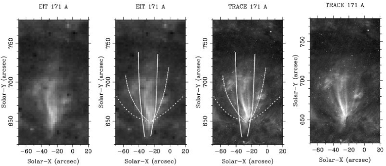
Figure 3: Two views of the same polar plume, imaged by TRACE and SOHO/EIT at 1999 Aug 27 19:00 UT, show the interplay between instrument resolution and derived structure size, even in features many pixels across. In the central panels, visual edges of the plume have been traced using the EIT data (solid lines), using the TRACE data with a conservative approach (dot-dashed lines), and using the TRACE data with the faintest visible edge at the extreme periphery of the plume (dashed lines). The outlines of the plume are surprisingly dependent on the instrument.

The visual result here is consistent with the results of Fuentes et al. (2006) in analyzing forward models of cylindrical structures near the TRACE resolution limit. Both results highlight the difficulty of separating the size of structures near the telescope’s ultimate limit. The Fuentes analysis uses the standard deviation of the feature’s brightness considered as a random-variable distribution, and is more rigorous than the present visual-width argument, but also demonstrates the importance of telescope PSF to the derived width of small structures in the corona from features in the image plane. Fuentes et al. argue that the PSF is small enough to not affect their main results on thread width versus altitude, but that argument depends strongly on the derived PSF of the instrument and may depend on other image interpretion effects that are not considered directly in that analysis.

In real data several effects worsen considerably the strength of image interpretation beyond a simple linear analysis of feature spreading by convolution with a PSF: most solar structures are not compact in cross-section; the image background contains features that can be confused with the feature of interest; and brightness variation across the cross-section of a linear feature may interact with background noise to produces spurious feature “edges” that are inconsistent with edges derived from the same structure viewed at a different resolution.

Figure 3 shows an example of the importance of resolution even to interpretation of structures that are significantly larger than the point-spread function of the observing telescope. Two images are shown of the same polar plume, taken with ~5 arc second resolution (by EIT) and with ~1 arc second resolution (by TRACE). The two images were collected within 30 seconds of one another and were both in the 171 Å EUV band, so the strongest differences between them are due to the instruments themselves. While some dark pixels are visible in the EIT image, and both images are subject to different patterns of cosmic ray hits, the largest difference is in the resolution of the images.

The EIT image shows the plume as a bright, thin feature embedded in a larger, round diffuse region on the Sun. With the higher resolution available to TRACE, we can identify many bright features in the plume and recognize that the plume has both a diffuse component and a threadlike component. By comparing resolution effects between the images at 5 arc second resolution and 1 arc second resolution near the limits of EIT, we can identify the sorts of visual effects that are to be expected near the resolution limit of TRACE.

The outer panels of Figure 3 are raw images; the inner panels are the same two images, but with co-aligned visually identified edges marked. The solid lines in the central panels show edge tracings using the EIT data alone; the dashed lines show edge tracings using the TRACE data, with the inner (dot-dash) set corresponding to the clearest visible edge of the plume as a whole and the outer (dash) set corresponding to the outermost visually identifiable edge.

The first, and most relevant, discrepancy to notice between the instruments is that the identified expansion factor is radically different between the two data sets. Although the plume is ~6 EIT pixels across at its brightest position (considerably larger than the EIT point-spread function) the expansion factor of the EIT edge tracing is less than two in the first 30 Mm of altitude. In the TRACE image there is both a diffuse component to the plume and also many small, bright threads that outline a much broader magnetic structure with a much larger overall expansion ratio than is visible with EIT.

The discrepancy in expansion ratio across the two instruments can be explained in terms of the interaction between resolution, geometric cross section, and background features. Near the center, the plume is denser and has a higher depth along the line-of-sight, making the core more visible than the exterior and giving rise to a visual edge with low expansion factor in the EIT image. At the base of the plume, resolution effects limit the smallest visible size of the overall structure, and higher up, only the brightest portion of the plume is visible and separable from the solar background, reducing the apparent cross section of the structure. These two effects conspire to produce a dramatically lower expansion ratio than is apparent in the TRACE data. Note that near the base of the plume the EIT visual edges cut laterally across field lines: the edge is defined by the gradient in intensity, which in turn depends both on variation in the visual chord length and also on the falling density versus altitude. The brightness at the base of the plume includes components both from the individual threads that are visible in the TRACE image and also from the diffuse material that fills the bulk of the plume’s volume; but even 30-40 arc seconds above the base of the plume, the diffuse emission falls below the intensity of background features and the threads dominate the visual appearance of the plume.

Other types of confusion are worth mention. Surrounding the base of the plume in the EIT image is a large, roughly circular region of diffuse emission that appears to be a supergranule or part of the network. Comparison with TRACE indicates that, although network brightenings are evident in the background, much of the brightness around the plume core is in fact due to the plume itself.

Additional problems with the lower resolution image include a lack of visual distinction between foreground and background objects. This leads both to an apparent twisting visible as a crescent-shaped bright feature in the plume core, and to an error in the position of the plume footpoint. At higher resolution the crescent is resolved as a coincidental alignment of a background network brightening and a foreground thread, while the base of the plume is seen to be confused with a foreground network brightening that extends the visual feature in the EIT image.

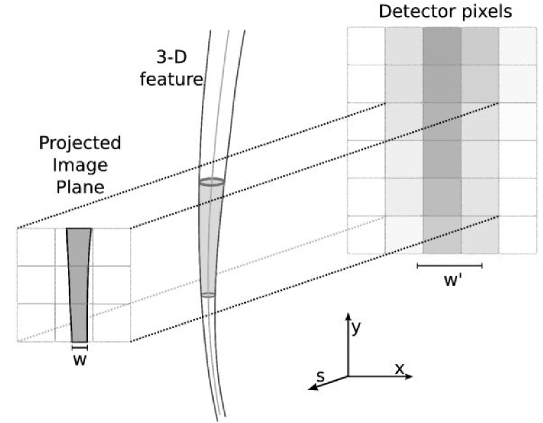
Figure 4: Geometry of optically thin solar imaging with finite resolution and pixel size. Features exist in 3-D (center) but images are brightness integrals along the line of sight $s$ (left). Physical instruments have instrumental spreading and pixel quantization (right), so that a feature with image plane width $w$ in fact yields a feature of apparent width $w^{\prime}$. The apparent brightness of the feature is proportional both to the emissivity within the feature and to the volume (shaded at center) of the feature within each pixel.

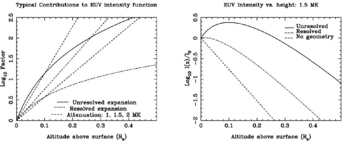
Figure 5: Unresolved, expanding filamentary structures explain the strong visibility of coronal features in EUV, out to about$1.3\,R_{\odot}$. LEFT: interplay of expansion for a typical active-region and three different scale heights (1.0 MK, 1.5 MK, and 2.0 MK). RIGHT: relative intensity versus height for structures at 1.5 MK, both with and without geometrical corrections. Without the geometric correction, coronal features are expected to be strongly attenuated above about 0.1 $R_{\odot}$ for all but the hottest features; with the correction, unresolved or barely-resolved features can be expected to remain visible out to ~0.3 $R_{\odot}$ (as is seen with EIT and TRACE).

The presence of various ambiguities and confusion in even quite large structures indicates that one must use extreme caution when analyzing structures that are close in size to the resolution of the source telescope, even when the apparent structure is several times larger than the PSF of the instrument. The reason is that visual context is needed to distinguish structural elements that give rise to the features in an image plane. Near the resolution limit, textural and alignment cues are not available because such cues are blurred out by the finite resolving power of the instrument.

In this case, the width of the EIT-determined plume structure is ~6 EIT pixels (15 arc seconds) near the base at solar-Y=660, quite a bit larger than the EIT PSF width of ~1-2 pixel (Delaboudiniere et al. (1995)); but improving the resolution by a factor of 3-5 (in the TRACE image) reveals the plume to be much wider: 30-60 arc seconds across at the same altitude.

3 Feature intensity profiles

EUV images from TRACE and EIT show structures extending up to about 0.2 $R_{\odot}$ from the surface of the Sun, or about 1.5-3 coronal scale heights (at temperatures of 1-2 MK); this is surprising because coronal volume emissivity in collisionally excited EUV lines varies as the square of the density, hence the emissivity ratio between the top and bottom of a hydrostatically supported active region loop should be of order $e^{-3}-e^{-6},$ i.e. at most a few times $10^{-2}$ (e.g. Aschwanden et al. 2000; Winebarger et al. 2003), rather than (as observed) of order $1$. The tallest active region loops, at  0.3 $R_{\odot}$, display yet more of a discrepancy. A more careful look at the geometry shows that the observed intensity of an unresolved coronal feature varies much more slowly than the plasma emissivity, resolving the discrepancy between the hydrostatic scale height and observed intensity profile, without dynamic or other support mechanisms to change the high altitude emissivity.

EUV imaging in optically thin, collisionally excited lines such as are visible through TRACE measures a brightness integral along the line of sight. The geometry of thin-feature imaging is summarized in Figure 4. The brightness at any location in the image plane of a non-vignetted EUV telescope may be described (DeForest et al. 1991) by a brightness integral:

$$\Phi(x,y)=tf^{2}\int ds\left(K_{tel}(T(s,x,y))n_{e}^{2}(s,x,y)\right)$$

where $\Phi$ is fluence (energy per unit area) on the detector plane; $x$ and $y$ are focal plane coordinates; $t$ is exposure time; $f$ is the f-ratio of the telescope; $s$ is distance along the line of sight; $K_{tel}$ is a temperature response kernel that includes the effects of telescope wavelength passband, atomic physics, and the solar elemental abundances; and $n_{e}$ is local electron density in the corona as a function of focal plane location and distance along the line of sight. For DEM-style analyses, the integral is rewritten, in the manner of Lebesgue, into an integral over T; but the simplest case is a single, compact structure at one location along the line of sight.

Consider a telescope pixel with a line of sight that includes a single elementary structure – an isothermal thread that approximates a long cylinder with slowly varying radius $r(s)$ along its length, with uniform density across its cross section, and with no other structures along the line of sight. If the thread is unresolved by the telescope, and extends along the $x$ axis, then the fluence $\Phi$ deposited in each pixel is given by:

$$\Phi_{ur}(x,y) = tf^{2}p\int\int dyds\left(K_{tel}(T_{struct})n_{e}^{2}\right)$$ (1)

$$=tf^{2}p\pi r^{2}\,K_{tel}(T_{struct})n_{e,struct}^{2}$$

$$\propto r^{2}n_{e,struct}^{2}$$

where $n_{e,struct}$ and $T_{struct}$ are the density and temperature inside the structure, $p$ is the linear size of a pixel, and $r$ is the diameter of the (unresolved) solar structure being observed.

Even if the structure is fully resolved and therefore the brightness is spread across more pixels as the radius increases, geometry still enters the brightness distribution as the depth of the feature varies. In a resolved structure the brightness scales as

$$\Phi_{r}(x,y)\propto rn_{e,struct}^{2}$$ (2)

under the same approximation as in Equation 1. Clearly, structures near the resolution limit of a given telescope will have a pixel brightness that varies between the 2nd and 1st powers of $r$ as the geometry transitions between the fully unresolved and fully resolved cases.

Consider, then, an unresolved coronal loop of temperature $10^{6}$K, height $0.2R_{\odot}$ (2.7 scale heights) and a linear expansion factor 8-10, typical of expansion ratios in modeled active region loops (J. Klimchuk, priv. comm.). Then the pixel brightness ratio $P_{top}/P_{base}$ is between $(8^{2})(e^{-5.4})$ and $(10^{2})(e^{-5.4})$, or 0.3-0.5; this is consistent with brightness ratios in active regions observed with TRACE. A naive treatment, ignoring geometry, might predict a brightness ratio of just $e^{-5.4}$, or $4\times 10^{-3}$, which is much more contrast than is actually observed.

Hence, for unresolved, isothermal, elementary coronal structures that expand with the bulk structure around them, we expect that

$$\frac{I_{ur}(z)}{I_{0}}\propto f_{local}^{2}(z)\,e^{-2z/h}$$ (3)

where $z$ is height above the surface of the Sun, $I(z)$ is the observed feature intensity in EUV, $I_{0}$ is its basal intensity, $f_{local}$ is the local linear expansion ratio introduced for coronal holes by Munro and Jackson (1977), and $h$ is the scale height (25-50 Mm for coronal plasma at 1-2 MK).

Combining Equation 3 with a typical feature expansion curve explains both the peculiar brightness of the EUV corona out to about 1.2-1.3 $R_{\odot}$ and its sudden disappearance above that height. Close to the surface, the expansion factor rises rapidly with altitude, canceling the density gradient with altitude; but farther away, the exponential falloff of density overwhelms the geometric effect. The balance is illustrated in Figure 5, which treats flux tubes in the field from a potential dipole embedded 50 Mm under the surface of the Sun; this field has a linear expansion ratio of 7.5 between the photosphere and 0.2 $R_{\odot}$.

It is important to note that even threads that are resolved near the top of an active region loop may not be resolved farther down. Such a partially-resolved structure will follow the “unresolved” intensity curves in Figure 5 near its footpoints, and steepen gradually to be parallel to the “resolved” intensity curve as the cross section exceeds the telescope’s minimum resolvable width. Both the “resolved” and “unresolved” curves fall off more slowly than the simple $e^{-2z/h}$ curve that might be expected for a constant-diameter feature, because of the increased depth at higher altitudes. Hence, all localized, optically thin structures that expand with altitude (even those which are resolved spatially) will have apparent intensity scale heights that are long compared to the coronal density scale height, simply due to the geometry of the structures. This depth effect is important to image analysis of large structures such as the diffuse brightening around active regions (e.g. Cirtain 2005), even though those structures may be fully resolved in the image data.

4 A hydrostatic active region model

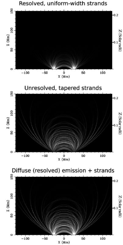
Figure 6: Rendered models of a hydrostatic active region: (TOP) constant-width threads; (CENTER) unresolved variable-width threads. (BOTTOM) A complete active region model including both diffuse (resolved) emission and unresolved variable-width bright threads with low filling factor.

To gain a better understanding of the simple analytic case above, I generated hydrostatic coronal models of a very simple active region by tracing a bundle of 300 random field lines through a potential dipole field, and modeling collisionally excited, optically thin EUV emission from a plasma structure associated with each of the field lines. Each thread is modeled as a hydrostatic plasma with randomly selected temperature between 1.0 - 1.5 MK and randomly selected base density that varies over a factor of 10. The emission is calculated using a simple broad-response-kernel approximation:

$$P_{pix}=\int d^{2}A_{pix}\left(\int ds\left(n_{e}^{2}\right)\right)$$ (4)

in which $P_{pix}$ is the optical power delivered to each pixel, $d^{2}A_{pix}$ represents integration over the area of the pixel in a perfect telescope, $ds$ is a coordinate along the line of sight, and $n_{e}$ is the modeled electron density. This is similar to the response-kernel method described above but neglects the $K_{tel}(T)$ temperature response kernel of the telescope (here approximated by selecting only features in a temperature range appropriate to TRACE Fe XII images). For a collection of slowly-varying elementary structures, and neglecting any background brightness, the triple integral over $d^{2}A_{pix}ds$ reduces to a sum over all features along the line of sight:

$$P_{pix}=\sum_{i}V_{i,pix}n_{e,i}(z)$$ (5)

where $i$ indexes all the features in the model, $V_{i,pix}$ is the volume occupied by the intersection of the pixel extended along its line of sight and the $i^{th}$ feature of interest, and $n_{e,i}$ is the density in the $i^{th}$ feature at the altitude of that intersection. The volume is determined by the length (measuring along the feature in 3-space) of the intersection, and by the cross-section of the feature. The features are treated as small flux tubes, so their cross sectional area is proportional to $1/B$, the reciprocal of the local field strength.

The top two images in Figure 6 show the results of the hydrostatic model for two feature geometries. In the top frame, the brightness at each pixel was calculated using a constant diameter for each thread (assumed to have circular cross section). In the center frame, the brightness was calculated using tapered (but still unresolved) flux tubes. The models are projected into the (X,Z) plane for the rendering, so that the height dependence can be seen. The brightness of the two simple models corresponds well to the plots in Figure 5.

The apparent increase in scale height of the threads in Figure 6(center) is only an optical illusion due to the small filling factor and high density of the structures. The hydrostatic scale height is approximately the same throughout the modeled corona (varying by only a factor of 1.5), so that the emissivity of the plasma in the threads must be very much brighter than that of the surrounding material. The thread brightness is comparable to the background brightness only because the underlying flux tube fills a small percentage of each pixel; this attenuates the total brightness of the thread, so that the underlying structure must be quite bright to be visible at all. However, the $n_{e}^{2}$ dependence of collisionally excited radiation accomplishes the job: to achieve an increase of 100 in volume emissivity it is only necessary to increase density (and hence pressure) by a factor of 10. In active region bases the average value of $\beta$ is of order $10^{-4}$ or lower, which might thus be raised to $10^{-3}$ in the dense structures. Hence, the structures may still be magnetically dominated and yet also be dense enough to be visible. The main practical limit to overall plasma density in each structure is the total energy input, which must balance the radiative losses along the entire length of the loop.

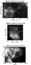
Figure 7: Three active region images seen with TRACE in the 195 Å EUV passband, selected for visual clarity of loop structures. Several hand-traced loops composed of filamentary threads are marked.

Put another way, the surprising aspect of Figure 6(center) is not that the tops of the thin structures are bright but rather that their bases are faint. In this model, they are strongly attenuated by the tapering geometry of the magnetic field.

Modeling only these super-bright unresolved elementary structures does not yield a realistic image of a typical active region, because the tapering of the structures produces footpoints that are too faint (though some active region loops do indeed appear to have fainter bases than tops in the EUV). That problem may be addressed by considering each active region to consist of a collection of very dense, unresolved flux tubes embedded in a larger, resolved volume with much lower density; this approach agrees with the experimental result by Cirtain (2005) that active regions have both fine and diffuse components. The bottom panel of Figure 6 demonstrates the result of summing the two types of emission, yielding a fair approximation of a typical active region’s brightness structure with minimal physics (only potential-like magnetic expansion factors and hydrostatic density profiles).

One may expect that emission from the base of the active region will be dominated by high-filling-factor plasma with close to the conventional density and temperature values, but that visual features at the top of the active region will be mainly small bright structures with similar scale height and much greater density compared to the bulk volume of the active region. In fact, the ratio of emission from large-scale spaces and unresolved threads is expected to be more or less the same at the top of the active region as a whole and at the bottom, but the expansion of the magnetic flux tubes between the bottom and the top allows the threads to be distinguished spatially at the top of the active region. At the base of the active region, both the bright flux tubes and the spaces between them are smaller and therefore superimposed by the telescope. There, the pixel brightness is dominated by the material between the threads, because of the much greater filling factor of the interthread material.

5 Elementary Structures seen with TRACE?

I studied the morphology of several active regions with threadlike loop structure observed in the EUV with TRACE. I present 8 typical cases in three separate active region complexes. The images were selected for visual clarity of the loop structures in the active region, and for variety of loop types. Each active region contained bright threads that were isolated enough to afford visual identification not only of the threads but also of complete bundles. Three active region images, and some loop identifications, are shown in Figure 7.

It is difficult to measure the taper of a curved coronal loop, so I traced out individual bright features with a simple point-and-click procedure, and then resampled the images to straighten the polygon by splicing the piecewise-linear segments into a straight line segment while retaining image scale. The resulting plots show the bright feature and its environs as a straight line, much like a navigational chart of a river. In these plots vertical is always a close approximation of the transverse direction, so the width of the composite loop of which each bright feature is a member is readily apparent.

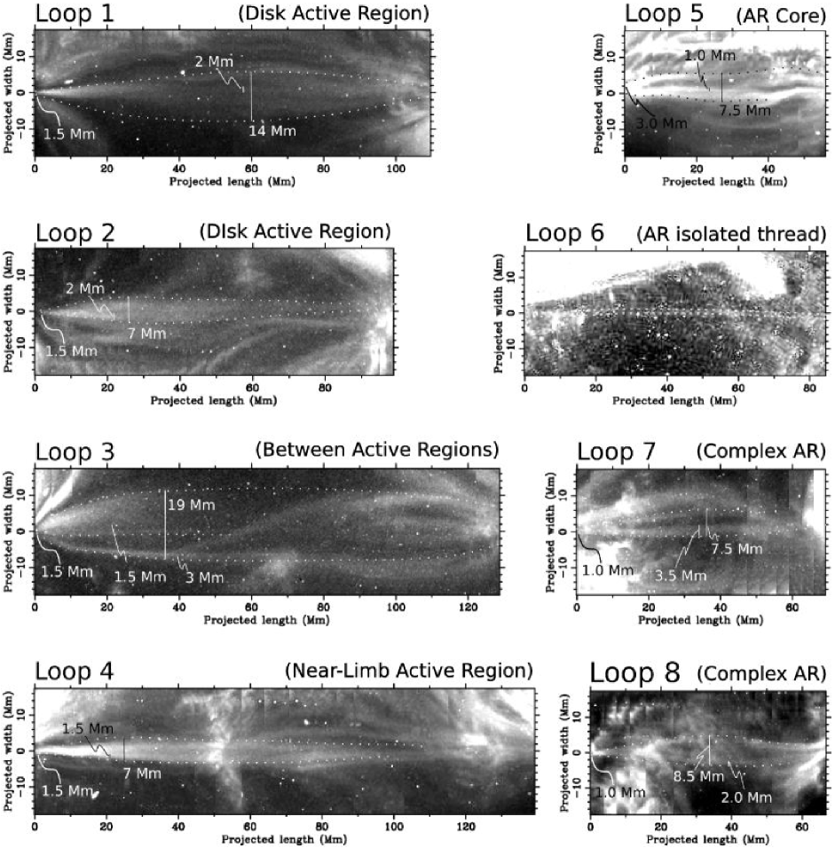
Figure 8: Loops from Figure 7, straightened along a hand-traced curve. Note the presence of small constant-apparent-width features near the telescope resolution limit, embedded within much larger variable-width loops. Tracings near the left side of each image are more to be trusted than those near the right. See text for full discussion.

I hand-traced the edges of the loop bundle containing each loop thread, yielding the curved dashed lines in Figure 8, and identified cross-sectional apparent sizes of both the bundle and thread at several points. I selected individual loops for clarity of features near one footpoint; that footpoint is always at the leftmost side of the image, so that tracings are more to be trusted on the left than on the right. That is in keeping with Fuentes & Klimchuk’s (2006) observation that features are difficult to trace footpoint-to-footpoint. All of the loop bundles contain several bright threads, each of which has similar appearance to the “elementary” structures identified by Aschwanden and Nightingale (2005); in fact, Loop 6 is one of the structures identified by them as elementary. Note that these constant-width threadlike features are at or near the telescope resolution limit and are therefore not easily distinguishable from much narrower structures that happen to not be resolved; in fact, near the base of each loop bundle the several threads appear to merge into a single bright feature with about the same width as the individual threads themselves. Further, although some of the features are clearly larger than the resolution limit near the top of the loop (for example, Loop 7), if in fact they taper with the surrounding bundle then each of them is much smaller than the resolution limit near the footpoint; treating the features as if they were resolved along their entire length thus results in a gross underestimate of the expansion factor within the thread, even for threads that are obviously resolved near their widest points.

In each loop (other than Loop 6) in Figure 8, the footpoint apparent width and the loop central apparent width have been marked. Without knowing the unresolved profile of the features it is difficult to know the effect of the TRACE point spread function, because feature profile strongly affects how the apparent width varies when a small feature is convolved with a comparably sized kernel. In a noise-free measurement, feature widths add in quadrature, but the presence of background beightness and the types of confusion demonstrated in Figure 3 the noise-free FWHM of a feature may be considerably different than its apparent visual width.

Taking the TRACE point spread function to be 2.375 pixels (0.83 Mm) in width (the average of the minor and major PSF axes given by Gburek, Sylwester, and Martens (2006)), and ignoring background or confusion effects in the features, it is possible to generate rough estimates of the real apparent widths of the structures that give rise to the features in Figure 8. Subtracting (in quadrature) the Gburek width of 0.83 Mm gives expansion ratios varying from 2.6 (in Loop 4) to 15.1 (in Loop 3), with a mean of 9.7 across all loops. These numbers should be considered estimates only, because of the issues outlined in the previous paragraph.

Loop 3 in particular is interesting because it has both a high expansion ratio and a faint thread with an apparent size of 1.5 Mm (estimated real size of 1.25 Mm using subtraction in quadrature). If we assume that the cross-section of Loop 3 is self-similar, scaling smoothly down to the footpoint, we find an estimate (which should be taken as an upper bound) of 80km for the size of elementary structures in the lower corona. Neglecting the point spread function entirely yields a more conservative upper bound estimate of 110km: if the underlying structure were larger at the base, it would appear wider near the top of the active region. We have thus derived an estimate of the size of TRACE-visible elementary structures at the base of the corona, using hypothesis that the structures are barely resolved by TRACE near the loop top but taper proportionally with their enclosing bundle as expected in a near-force-free plasma.

The 110km upper bound based on morphological taper can be corroborated by the brightness profile of small, long, isolated features such as that in Loop 6. Such features (dubbed “elementary” by Aschwanden and Nightingale (2005)) have constant apparent widths of ~1.5-2Mm, maximum altitudes of ~0.1 $R_{\odot}$, and nearly constant brightness along their length. If indeed these very long, very fine features are unresolved and supported hydrostatically, then their footpoint sizes must be well under 100km to sustain the brightness uniformity across their several scale heights of altitude extent.

Using the fact that the structures are bright enough to be visible with TRACE, we can also derive a lower bound on their size. The limiting minimum size of a particular observed structure is set by the need to maintain $\beta\lesssim 1$ near the footpoint of the structures while emitting sufficient EUV photons per unit volume to be visible against nearby resolved structures. The smaller the structure, the denser the plasma must be, with $\beta\sim 1$ representing a practical maximum pressure (and density) for the plasma.

Taking $B=1000G$, $\beta=1$, and $T=10^{6}K$ at the base of the corona over a sunspot, one finds a maximum electron density of $10^{14}cm^{-3}$, compared to a “background” diffuse density of $10^{10}cm^{-3}-10^{11}cm^{-3}$ in the bases of active regions; this sets the minimum size to a few $\times 10^{-2}$ TRACE pixels, or ~10 km, at the base of the active region. If the faint structure at the center of Loop 3 (for example) were that narrow at its base, it would be visible with about the correct brightness and an actual width at its top of ~150 km (0.5 TRACE pixel), which is consistent with the existing apparent width of 2 diagonal TRACE pixels. Hence, elementary structures accessible to detection by TRACE most likely have a cross-field scale between 10-100 km at the base of the corona. To fully resolve such structures would require 15-150 milliarcsecond resolution from near Earth, or 6 arcsecond resolution from a hypothetical solar probe spacecraft located at 3-20 $R_{\odot}$.

One might not expect that many currently-visible features are much smaller than 75km (the estimated size of Loop 3) at their bases: Klimchuk (2006, priv. comm.) has pointed out that selecting the brightest, clearest fine structures to study is equivalent to selecting structures close to the resolution limit of the telescope. This selection effect may bias the current result toward large (~75km) filamentary structures.

6 Discussion & Conclusions

I have demonstrated that spatial resolution effects are sufficient to explain both the peculiar cross-sectional structure and extended height of active region loops as seen with current EUV imagers, using only hydrostatic equilibrium of the plasma contained in the loops and geometric effects due to the non-resolved nature of the loops. This offers simple explanations for several current theoretical difficulties with observed active region loops, giving weight to the hypothesis that elementary coronal structures are simply not resolved but are affected by geometric effects that are not distinguishable to current imagers.

The geometric effects attenuate the brightness of unresolved structures near their bases. If ignored, this can result in a gross underestimate of the basal density in the structures and hence an overestimate of the pressure scale height within them. More generally, semi-empirical analyses that compare the subjective appearance of forward-modeled intensity data with solar images will yield incorrect results if the geometry of unresolved structures is not incorporated in the model. While some analyses (e.g. Fuentes et al. 2006) consider spatial resolution issues, all current analysis of active region loops seems to use the uniform apparent widths of narrow coronal threads in TRACE images as evidence of the uniformity of the corresponding structures’ actual widths. This inference gives rise to many difficulties in the understanding of active region loops, and it is arguably the weakest link in the current chain of inference from observational results to comparison with theory. Therefore the question of loop width requires extremely careful consideration.

In particular, by comparing simultaneous images of a single feature from both EIT and TRACE, I have shown that resolution effects can cause confusion in visual analysis even of structures up to ~6x the FWHM of the pixel-convolved PSF of an EUV imaging instrument (EIT). One may reasonably conclude that structures with apparent sizes below about 6x the FWHM of the TRACE PSF (~13 TRACE pixels) may also be subject to such ambiguity and confusion. Simple analysis of the images themselves cannot rule out such confusion effects, so that the sizes and even unique identifications of features smaller than about 4-5 Mm across are only weakly supported by image data from TRACE.

It is important to understand that any difficulty with interpreting TRACE images of small features is not isolated to that instrument: imaging distributed, optically thin objects is difficult, and near the resolution limit of any telescope the interpretation of the images becomes strongly model dependent. Forward modeling of the images produced by a particular type of structure is not sufficient reason to conclude that the features observed in real data correspond to resolved structures on the Sun. Better resolution or, at a bare minimum, truly adversarial hare-and-hounds type exercises are required.

Furthermore, even fully resolving a coronal structure is not sufficient reason to ignore geometric intensity effects. Even fully resolved loops vary in thickness along the line of sight and that variation must be considered and modeled in the course of drawing inferences about scale height and other effects from image data. Geometric effects in fully resolved structures are not as strong as in unresolved structures, but are sufficiently important to feature brightness profiles that they may act as a trap for the unwary.

This analysis is timely in part because much recent work attempts to find physical mechanisms on the Sun for phenomena that could potentially be understood in terms of instrumental effects. I have demonstrated that thread morphology in active region loops (and, by extension, in similar structures such as quiet sun loops and polar plumes) is not well constrained by current imaging instruments. Taking possible resolution effects into account renders the imaging data consistent with a naive hydrostatic model of the solar corona and explains both the high feature contrast and relatively uniform height (about $0.2-0.3R_{\odot}$) of nearly all large, bright coronal features seen with EUV imaging instruments.

Recent work by Aschwanden (2005) and Aschwanden and Nightingale (2005) describes imaging of individual elementary loop structures in the corona, based on differential emission measure analysis of individual TRACE images. Similar filter-ratio analyses (e.g. DeForest 1995; Kankelborg 1996) have found “elementary” EUV structures (in the sense of being nearly isothermal in multiple-passband analyses of EUV telescope data) that were resolved by the Multi-Spectral Solar Telescope Array (Walker et al. (1991)) on spatial scales of ~10 arcseconds, close to the resolution limit of that instrument; but it is now obvious from the TRACE data that multiple arcsecond size structures are essentially always inhomogeneous.

The present analysis suggests that recent results regarding coronal elementary structures may be similar to the older ones: the structures are likely not resolved by TRACE in the usual sense. I suggest that, like earlier measurements, thread features in TRACE images are most likely distinguished merely by virtue of containing a single bright structure (or group of structures at a particular temperature) that happens to be much denser and brighter than other adjacent magnetic structures passing through the same pixels in the image plane.

What is different between the 1-arcsecond class data from TRACE and images from prior instruments is that TRACE has sufficient resolution to distinguish some of the bundled nature of coronal loops, allowing the use of the taper of those bundles to infer something about the fundamental scale of the corona. This was not possible with images with multiple arcsecond resolution.

Further, the hypothesis that the small threads seen with TRACE are both elementary (isothermal and uniform density across the structure) and unresolved also yields an estimate of the fundamental size scale at the base of the corona based on the smallest features seen higher up. That estimate (10km-100km) suggests that a high resolution imager or solar probe mission will be needed to resolve such elementary structures. The upper size figure is derived (in §5) from direct morphological scaling of observed threads within active region loops, and the lower figure is derived from brightness considerations and the need to confine the plasma magnetically: elementary structures could in principle be smaller still, but they would most likely be too faint to see with TRACE. The size range of 10-100 km is consistent with reconnective heating induced by the motion of g-band bright points seen in the intergranular lanes of quiet sun and decaying active regions, or by the motion of penumbral rolls and similar very fine scale features near sunspots, suggesting that microflare mechanisms driven by local surface motion may be responsible for the large scale threaded appearance of active regions.

Taking the corona to have both a low-filling-factor, high density component and a high-filling-factor, lower density component (e.g. Cirtain 2005 and references therein) yields an elegant explanation for the overall appearance and high feature contrast of the EUV corona. In particular, bright structures on the limb of full-disk images from EIT and from TRACE are easily seen to extend up to  0.3 $R_{\odot}$ above the surface of the Sun but fade rapidly into the background above that altitude. This effect may be seen as a direct result of the interplay between expansion of fine structures and exponential decrease in their density as in Figure 5.

Finally, very dense, unresolved structures could account for the surprisingly high intensity contrast of small features seen throughout the corona with EUV imagers. If bright coronal loops do indeed have emissivities 100x-1000x higher than the surrounding “diffuse” corona, and are indeed tapered below the resolution limit of the telescope, then the interplay of resolution and geometric effects accounts very handily for two surprising aspects of EUV loops seen with EIT, TRACE and other EUV telescopes: the high intensity contrast (order unity) of coronal loops at moderate altitudes of 0.1-0.3 $R_{\odot}$ compared to the background corona, despite a factor-of-100 difference in length between the portion of the line of sight inside the EIT loop and the portion in the surrounding corona; and the comparatively low intensity contrast (of about unity) of coronal loop footpoints compared to the surrounding corona, despite large differences in altitude between the top and bottom of the loop. The loops (and their components, TRACE threads) may be understood as very bright, unresolved structures that taper with altitude, so that their integrated brightness close to the bottom of the corona is quite small despite even higher emissivity than at moderate altitudes of 0.2-0.3 $R_{\odot}$

Temporal behavior can be used to test the importance of geometric effects and very dense threads, even without a high resolution telescope. The thermodynamics of long active region loops are dominated by radiative cooling, with smaller contributions from conduction and (in the presence of flow) advection. Because the emissivity of the plasma varies as $n_{e}^{2}$, the cooling time scales inversely as density. The radiative cooling time of typical active region plasma is order of 1000 seconds, which is consistent with the typical fading time reported by Schrijver et al. (1999) of  500 seconds. If threads are 10x denser than the surrounding material, the cooling time should be correspondingly shorter - on the order of perhaps 60 seconds. This is not necessarily inconsistent if the heating mechanism of the threads has a longer time scale and the threads themselves are close to thermal equilibrium. However, if no such fast-fading threads are ever observed, that would weakly falsify the proposition that coronal threads are currently-unresolved filamentary structures. Contrariwise, if even a small subset of active region EUV threads are shown to fade with time scales much faster than 5 minutes, that would support the proposition.

Throughout this discussion I have used the word “thread” (and the related phrases “threaded”, “multithreaded”, and “threadlike”) rather than the more conventional “filamentary structure”. The latter phrase is cumbersome and also leads to confusion with filaments; while the more recent alternative, “elementary structure”, has theoretical/modeling implications unrelated to the simple appearance of the features. Similarly, “loop” is not specific to arcsecond scale features observed in high resolution EUV images from instruments like TRACE, because it may also be considered to apply to larger bundles of threads, which form 10-30 arcsecond scale features in moderate resolution EUV images. I suggest using “thread” as a purely observational term to describe small, apparently-constant-width structures within coronal loops and other features in the image plane of a telescope, because the word is short, pithy, easy to remember via analogy to textiles in everyday experience, and not (yet) laden with non-observational nuance.

References

- Aschwanden [2005] M. J. Aschwanden. ApJ, 634: L193–L196, 2005.
- Aschwanden and Nightingale [2005] M. J. Aschwanden and R. W. Nightingale. ApJ, 633: 499–517, 2005.
- Aschwanden and Nitta [2000] M. J. Aschwanden and N. Nitta. ApJ, 535: L59–L62, 2000.
- Aschwanden et al. [2000] M. J. Aschwanden, R. W. Nightingale, and D. Alexander. ApJ, 541: 1059–1077, 2000.
- Cirtain [2005] J. W. Cirtain. The Solar EUV Corona: Resolved Loops and the Unresolved Active Region Corona. Ph.D. dissertation, Montana State University, 2005.
- DeForest [1995] C. E. DeForest. Ph.D. dissertation, Stanford University, 1995.
- DeForest et al. [1991] C. E. DeForest, C. C. Kankelborg, M. J. Allen, E. S. Paris, T. D. Willis, J. F. Lindblom, R. H. O’Neal, A. B. C. Walker, T. W. Barbee, and R. B. Hoover. Optical Engineering, 30: 1125–1133, 1991.
- Delaboudiniere et al. [1995] J.-P. Delaboudinière, G. E. Artzner, J. Brunaud, A. H. Gabriel, J. F. Hochedez, F. Millier, X. Y. Song, B. Au, K. P. Dere, R. A. Howard, R. Kreplin, D. J. Michels, J. D. Moses, J. M. Defise, C. Jamar, P. Rochus, J. P. Chauvineau, J. P. Marioge, R. C. Catura, J. R. Lemen, L. Shing, R. A. Stern, J. B. Gurman, W. M. Neupert, A. Maucherat, F. Clette, P. Cugnon, and E. L. van Dessel. Sol. Phys., 162: 291–312, 1995.
- Doyle et al. [1985] J. G. Doyle, H. E. Mason, and J. E. Vernazza. A&A, 150: 69–75, 1985.
- Feldman [1987] U. Feldman. Atlas of extreme ultraviolet spectroheliograms from 170 to 625 A. Volume 1; Volume 2. Washington, Naval Research Laboratory, E.O. Hulburt Center, 1987, edited by Feldman, Uri, 1987.
- Fredvik et al. [2002] T. Fredvik, O. Kjeldseth-Moe, S. V. H. Haugan, P. Brekke, J. B. Gurman, and K. Wilhelm. Advances in Space Research, 30: 635–640, 2002.
- Fuentes et al. [2006] M. C. L. Fuentes, J. A. Klimchuk, and P. Démoulin. ApJ, 639: 459–474, 2006. doi: 10.1086/499155.
- Gburek, Sylwester, and Martens [2006] S. Gburek, J. Sylwester, and P. Martens. Sol. Phys., in press.
- Golub and Pasachoff [1997] L. Golub and J. M. Pasachoff. The Solar Corona. The Solar Corona, by Leon Golub and Jay M. Pasachoff, p. 233. ISBN 0521480825. Cambridge, UK: Cambridge University Press., 1997.
- Golub et al. [1999] L. Golub, J. Bookbinder, E. Deluca, M. Karovska, H. Warren, C. J. Schrijver, R. Shine, T. Tarbell, A. Title, J. Wolfson, B. Handy, and C. Kankelborg. A new view of the solar corona from the transition region and coronal explorer (TRACE). Physics of Plasmas, volume 6(5): 2205-2216.
- Handy et al. [1998] B. N. Handy, M. E. Bruner, T. D. Tarbell, A. M. Title, C. J. Wolfson, M. J. Laforge, and J. J. Oliver. UV Observations with the Transition Region and Coronal Explorer. Sol. Phys., 183: 29–43, 1998.
- Harra et al. [2004] L. K. Harra, C. H. Mandrini, and S. A. Matthews. What causes solar active region loops to exist at transition region temperatures? Sol. Phys., 223: 57–76, 2004. doi: 10.1007/s11207-004-0937-x.
- Kankelborg [1996] C. C. Kankelborg. Ph.D. Thesis, 1996.
- Karpen et al. [2001] J. T. Karpen, S. K. Antiochos, M. Hohensee, J. A. Klimchuk, and P. J. MacNeice. Are Magnetic Dips Necessary for Prominence Formation? ApJ, 553: L85–L88, 2001. doi: 10.1086/320497.
- Munro and Jackson [1977] R. H. Munro and B. V. Jackson. Physical properties of a polar coronal hole from 2 to 5 solar radii. ApJ, 213: 874–+, 1977.
- Schrijver et al. [1999] C. J. Schrijver et al. A new view of the solar outer atmosphere by the Transition Region and Coronal Explorer Sol. Phys., 187: 261.
- Tousey et al. [1977] R. Tousey, J.-D. F. Bartoe, G. E. Brueckner, and J. D. Purcell. Extreme ultraviolet spectroheliograph ATM experiment S082A. Appl. Opt., 16: 870–878, 1977.
- Walker et al. [1991] A. B. C. Walker, J. F. Lindblom, J. G. Timothy, R. B. Hoover, T. W. Barbee, P. C. Baker, and F. R. Powell. High resolution imaging with multilayer soft X-ray, EUV and FUV telescopes of modest aperture and cost. In P. Y. Bely and J. B. Breckinridge, editors, Space astronomical telescopes and instruments; Proceedings of the Meeting, Orlando, FL, Apr. 1-4, 1991 (A92-45151 19-89). Bellingham, WA, Society of Photo-Optical Instrumentation Engineers, 1991, p. 320-333., pages 320–333, 1991.
- Warren and Winebarger [2003] H. P. Warren and A. R. Winebarger. Density and Temperature Measurements in a Solar Active Region. ApJ, 596: L113–L116, 2003. doi: 10.1086/379094.
- Winebarger et al. [2003] A. R. Winebarger, H. P. Warren, and J. T. Mariska. Transition Region and Coronal Explorer and Soft X-Ray Telescope Active Region Loop Observations: Comparisons with Static Solutions of the Hydrodynamic Equations. ApJ, 587: 439–449, 2003. doi: 10.1086/368017.