Testing the standard fireball model of GRBs using late X-ray afterglows measured by Swift

Abstract

We show that all X-ray decay curves of GRBs measured by Swift can be fitted using one or two components both of which have exactly the same functional form comprised of an early falling exponential phase followed by a power law decay. The 1st component contains the prompt $\gamma$-ray emission and the initial X-ray decay. The 2nd component appears later, has a much longer duration and is present for $\approx 80\%$ of GRBs. It most likely arises from the external shock which eventually develops into the X-ray afterglow. In the remaining $\approx 20\%$ of GRBs the initial X-ray decay of the 1st component fades more slowly than the 2nd and dominates at late times to form an afterglow but it is not clear what the origin of this emission is.

The temporal decay parameters and $\gamma$/X-ray spectral indices derived for 107 GRBs are compared to the expectations of the standard fireball model including a search for possible “jet breaks”. For $\sim 50\%$ of GRBs the observed afterglow is in accord with the model but for the rest the temporal and spectral indices do not conform to the expected closure relations and are suggestive of continued, late, energy injection. We identify a few possible jet breaks but there are many examples where such breaks are predicted but are absent.

The time, $T_{a}$, at which the exponential phase of the 2nd component changes to a final powerlaw decay afterglow is correlated with the peak of the $\gamma$-ray spectrum, $E_{peak}$. This is analogous to the Ghirlanda relation, indicating that this time is in some way related to optically observed break times measured for pre-Swift bursts. Many optical breaks have previously been identified as jet breaks but the differences seen between X-ray and optical afterglows suggest that this is not the explanation.

1 Introduction

The standard fireball shock model of GRBs (Mészáros 2002 and references therein) predicts that a broadband continuum afterglow spectrum is expected to arise from an external shock when the relativistically expanding fireball is decelerated by the surrounding low density medium. As relativistic electrons, accelerated in the shock to form a power law energy spectrum, spiral in the co-moving magnetic field we should see a characteristic fading synchroton radiation spectrum stretching from radio frequencies through the IR, optical and UV bands in to an X-ray and gamma ray high energy tail. The detailed form of the expected afterglow spectrum and its evolution are described by Sari, Piran and Narayan (1998) and Wijers and Galama (1999).

X-ray afterglows of GRBs were first detected by the Beppo-SAX satellite (1996-2002) and the detection of GRB970228 (Costa et al. 1997) and other X-ray afterglows provided positions of sufficient accuracy to enable follow-up ground-based optical observations. Faint optical afterglows were discovered and it was soon established that GRBs occurred at comological distances. The first redshift, z=0.835, was measured for GRB970508 (Metzger et al. 1997). A connection between GRBs and supernovae was revealed by observations of GRB980425/SN1998bw (Galama et al. 1998, Kulkarni et al. 1998) although the supernovae associated with GRBs showed very high expansion velocities (tens of thousands of kilometers per second) and were given a new classification of hypernovae. The XMM-Newton observatory also detected X-ray afterglows. In particular GRB030329 confirmed the hypernova connection (Tiengo et al. 2003, Stanek et al. 2003, Hjorth et al, 2003) and multiwavelength observations and analysis of this bright afterglow and similar events (Harrison et al. 2001, Panaitescu & Kumar 2001, 2002, 2003, Willingale et al. 2004) established that afterglows were broadly consistent with the expected synchrotron spectrum and temporal evolution.

If the relativistic outflow is collimated in the form of a jet then we expect to see an achromatic break in the decay at time $t_{j}$ days after the burst when the edge of the jet becomes visible (Rhoads 1997, 1999). Many optical observations of GRB afterglow decays exhibit a break a few days after the initial burst, which is identified with a jet break, consistent with a collimation angle, $\theta_{j}$ $\sim 3-40$ degrees (Frail et al. 2001, Bloom et al. 2003). Assuming the fireball emits a fraction $\eta_{\gamma}$ of its kinetic energy in the prompt $\gamma$-ray emission and the circumburst medium has constant number density $n$ the collimation angle is given by

$$\theta_{j}=0.161\left(\frac{t_{j}}{1+z}\right)^{3/8}\left(\frac{n\eta_{\gamma}}{E_{iso}}\right)^{1/8}$$ (1)

where z is the redshift, and $E_{iso}$ is the total energy in $\gamma$-rays in units of $10^{52}$ ergs calculated assuming the emission is isotropic (Sari et al. 1999). The collimation-corrected energy is then $E_{\gamma}=E_{iso}(1-\cos\theta_{j})$ and this shows a tight correlation with the peak energy of the spectrum in the source-frame, $E_{peak}^{src}\propto E_{\gamma}^{0.7}$ (the Ghirlanda relation: Ghirlanda et al. 2004). Jet breaks seen in the optical should also be observed, simultaneously, in the X-ray band.

Prior to the launch of Swift (Gehrels et al. 2004, Burrows et al. 2005) both X-ray and optical follow-up observations of GRBs and their afterglows were limited to late times greater than several hours and often a day or more after the GRB trigger. Since launch, Swift has detected an average of 2 GRBs per week and we now have a sample of over 100 GRBs for which we have quasi-continuous coverage in the X-ray band in the range $\sim 100$ to $\sim 10^{6}$ seconds after the initial trigger. The aim of this paper is to compare the observed X-ray afterglows with the expectations of the standard model. One possible approach is to correlate the behaviour seen in the X-ray band with simultaneous optical measurements. Panaitescu et al. (2006) present an analysis for 6 GRBs detected by Swift noting that, contrary to expectation, temporal breaks in the X-ray band were not seen simultaneously in the optical. Another approach is to use the Ghirlanda relation to predict the time of expected jet breaks for Swift GRBs for which we have redshifts and then look to see if such breaks were observed. Sato et al. (2006) applied this to 3 bursts without success and concluded these bursts indicate a large scatter in the Ghirlanda relation. A third possible approach, presented here, is to make a systematic statistical study of the structure and evolution of a large sample of X-ray decay curves (including the method employed by Sato).

2 The functional form of X-ray decays seen by Swift

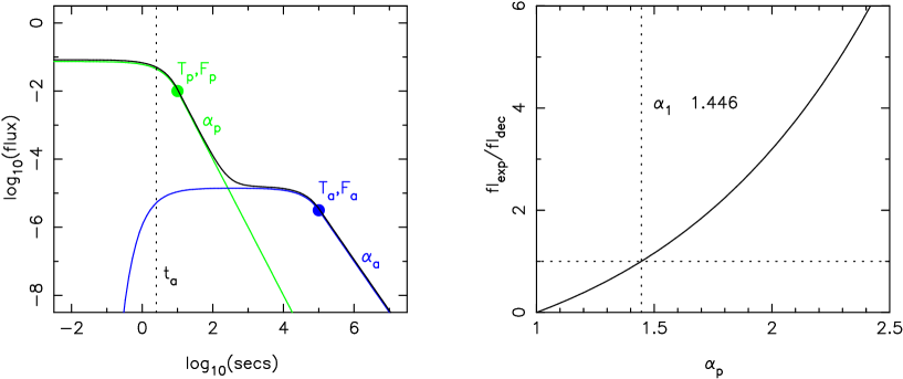
Figure 1: Left: The functional form of the decay and the fitted parameters. The prompt component (green) has no rise because time zero is set at the peak. The afterglow component (blue) rises at time $t_{a}$ as shown. Right: the ratio of the fluence in the exponential portion of the light curve to that in the power law decay as a function of $\alpha_{p}$. See Equations 3, 4 and 6.

An analysis of a sample of 40 X-ray decays observed by Swift by O’Brien et al. (2006), demonstrated that they all followed a similar pattern comprising an exponential decay in the prompt phase which relaxes to a power law decay at a time $T_{p}$. In most cases this initial power law decay flattens into a plateau or shallow decay which then gradually steepens and establishes a final afterglow power law decay at time $T_{a}$. Fig. 1 shows a schematic of the decay profile and the disposition of $T_{p}$ and $T_{a}$. Such behaviour is consistent with the presence of two emission components that overlap in time; a short duration prompt emission followed by an initial power law decay and designated by the subscript “p” and a much longer duration low luminousity afterglow component which starts as a slowly decaying plateau and ends with a steeper powerlaw, designated by the subscript “a”. The analysis reported by O’Brien et al. (2006) concentrated on the properties of the prompt “p” component and produced an estimate of $T_{p}$ using a scaled version of each X-ray light curve. In this paper we turn our attention to the later development of X-ray light curves and employ a function fitting procedure to estimate the parameters associated with both the prompt and afterglow components.

We have found that both components are well fitted by the same functional form:

$$f_{c}(t)=F_{c}\exp\left(\alpha_{c}-\frac{t\alpha_{c}}{T_{c}}\right)\exp\left(\frac{-t_{c}}{t}\right),\>\>t<T_{c}$$

$$f_{c}(t)=F_{c}\left(\frac{t}{T_{c}}\right)^{-\alpha_{c}}\exp\left(\frac{-t_{c}}{t}\right),\>\>t\geq T_{c}$$ (2)

The transition from the exponential to the power law occurs at the point $(T_{c},F_{c})$ where the two functional sections have the same value and gradient. The parameter $\alpha_{c}$ determines both the time constant of the exponential decay, $T_{c}/\alpha_{c}$, and the temporal decay index of the power law. The time $t_{c}$ marks the the initial rise and the maximum flux occurs at $t=\sqrt{t_{c}T_{c}/\alpha_{c}}$.

Having established this generic behaviour we have fitted the X-ray decay curves of all 107 GRBs detected by both the BAT and XRT on Swift up to August 1st 2006 using two components of the form $f(t)=f_{p}(t)+f_{a}(t)$. Parameters with suffix $p$ ($T_{p}$,…) refer to the prompt component and those with suffix $a$ ($T_{a}$,…) the afterglow component. Fig. 1 illustrates the functional form of the two components.

The X-ray light curves were formed from the combination of BAT and XRT data as described by O’Brien et al. (2006). The conventional prompt emission, seen predominantly by the BAT, occurs for $t<T_{p}$ and the plateau/shallow decay phase, seen by the XRT, at $t<T_{a}$. The fits were produced in two stages. The first stage used the BAT trigger time as time zero, $t_{0}$. In this fit the term $\exp(-t_{p}/t)$ was included in the prompt function $f_{p}$ so that a peak position was found for the prompt emission. This peak time was then used as time zero and a second fit done with $t_{p}=0$ (i.e. without an initial rise in the prompt component). Following this two stage procedure ensures that the prompt power law index fitted, $\alpha_{p}$, is referenced with respect to the estimated peak time rather than the somewhat arbitary BAT trigger time. In most cases the time of the initial rise, $t_{a}$, of the afterglow component, $f_{a}(t)$, was fixed at the transition time of the prompt emission $t_{a}=T_{p}$. In a few cases this was shifted to later times because a small dip was apparent in the light curves before the start of the plateau or the plateau started particularly early. There was no case in which the two components were sufficiently well separated such that this time could be fitted as a free parameter. i.e. we are unable to see the rise of the afterglow component because the prompt component always dominates/persists at early times and $t_{a}$ could be much less than $T_{p}$ for most GRBs. Many of the decays exhibit flares towards the end of the prompt phase, during the initial power law decay, on the plateau and even in the final decay phase. All large flares were masked out of the fitting procedure. Although apparently bright, such flares account for only $\sim 10\%$ of the total fluence in most cases.

Chi-squared fitting was performed in log(flux) vs. log(time) space using the parameters $\log_{10}(T_{p})$, $\log_{10}(T_{a})$ and logs of the products, i.e. $\log_{10}(F_{p}T_{p})$ and $\log_{10}(F_{a}T_{a})$. The error estimation therefore produced a statistical error on the product of flux and time directly and these products could then be used to calculate the fluence and an associated fluence error in each of the components. The fluences of the prompt exponential and prompt powerlaw decay phases are

$$fl_{exp}=\frac{F_{p}T_{p}}{\alpha_{p}}(\exp(\alpha_{p})-1)$$ (3)

$$fl_{dec}=\frac{F_{p}T_{p}}{\alpha_{p}-1}\left(1-\left(\frac{T_{p}}{t_{max}}\right)^{\alpha_{p}-1}\right)$$ (4)

where $t_{max}(>T_{p})$ is the end of the light curve or some late time when the decay is deemed to have terminated. If $\alpha_{p}>>1$ then $t_{max}$ can be set to infinity. The fluence of the exponential phase in the afterglow component is reduced by the initial exponential rise factor $\exp(-t_{a}/t)$ and is given approximately by

$$fl_{exp}=\frac{F_{a}T_{a}}{\alpha_{a}}\left(\exp(\alpha_{a}\left(1-\frac{t_{a}}{T_{a}}\right))-1\right)$$ (5)

The inclusion of the exponential rise term has negligible effect on the fluence of the decay phase. Another way of viewing $\alpha_{p}$ (or $\alpha_{a}$) is that it controls the ratio of fluences seen from the exponential phase, $t<T_{p}$ (or $T_{a}$), and the decay phase, $t>T_{p}$ (or $T_{a}$). If the peak time, $t_{p}$, is zero and $t_{max}\rightarrow\infty$ then the ratio of the fluences for the prompt component is

$$\frac{fl_{exp}}{fl_{dec}}=\frac{(\exp(\alpha_{p})-1)(\alpha_{p}-1)}{\alpha_{p}}$$ (6)

and $fl_{exp}/fl_{dec}=1$ when $\alpha_{p}=\alpha_{1}\equiv 1.446$. If $\alpha_{p}<<\alpha_{1}$ then the decay is slow and most of the energy appears for $t>T_{p}$ in the power law decay. If $\alpha_{p}>>\alpha_{1}$ then the decay is fast and most of the energy appears for $t<T_{p}$ in the early exponential phase. Fig. 1 shows the fluence ratio as a function of $\alpha_{p}$. A very similar expression holds for the fluence ratio of the afterglow component but this includes a minor adjustment because of the initial rise in the exponential phase, $t<t_{a}$.

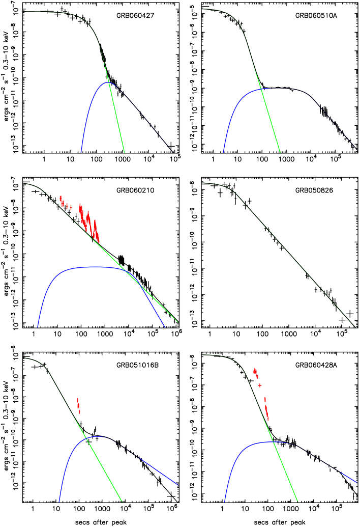
Figure 2: Examples of the fits to X-ray decay curves. The prompt and afterglow component functions are plotted in the same way as in Fig. 1. Top panels: the most common type in which the 2nd, afterglow, component dominates at late times. Middle panel left: a two component fit in which the afterglow component forms a bump in the decay but the extrapolation of the prompt component decay dominates at late times. Middle panel right: a single component fit, requiring no afterglow component. Bottom panels: two examples of fits which include a late temporal break. Flares are plotted in red and were excluded from the fitting procedure.

Table 1 lists the fitted parameters for all the GRBs in the sample. The type of decay fit (D) is also listed in Table 3. Of the 107 decays fitted, 85 required two components in which the afterglow component was dominant at the end of the observed light curve (D=1). In these cases the decay index of the prompt phase, $\alpha_{p}$ was usually greater than the $\alpha_{a}$ the final decay index of the afterglow. In a further 6 cases two components were required but the second component appeared as a hump in the middle of the initial decay and the prompt component reappeared and dominated again towards the end (D=2); these are marked^∗ in Table 1. For these objects the prompt decay is slow, $\alpha_{p}<1.5$, and it is usually the case that $\alpha_{p}<\alpha_{a}$. The remaining 16 required only one component (D=3) and did not exhibit a plateau phase with a subsequent power law decay. In 9 of these cases this was probably because the object was faint and the prompt emission faded below the XRT detection threshold before a putative plateau could be recognised. Fig. 2 shows typical examples of all these fitted types.

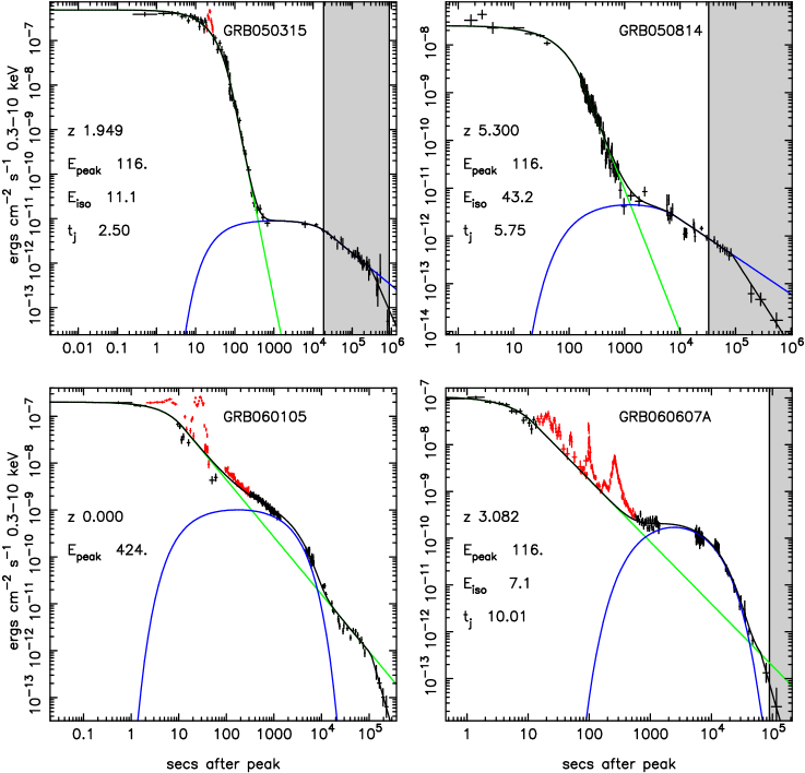
Figure 8: X-ray decays in which there is potential jet break. The shaded area indicates the expected range of $t_{j}$ calculated using the Ghirlanda relation for GRBs with a measured redshift. None of these has a measured $E_{peak}$ value so $116\pm 50$ keV has been assumed (see Section 5). The estimated $E_{iso}$ ($10^{52}$ ergs) and predicted $t_{j}$ (days) are listed on the left.

For 99 of the 107 GRBs the latter stages of the light curve are well represented by the one or two component functional fit described above. For those with two components the plateau gradually steepens in the exponential phase, $t<T_{a}$, and relaxes into a simple power law for $t\geq T_{a}$. For those with one component the prompt emission turns over into a final power law decay at $t\geq T_{p}$. However, in 8 cases there is clear evidence for a late temporal break. For these objects two extra parameters were included in the fit, a final break at time $T_{b}$ and a decay index $\alpha_{b}$ for $t>T_{b}$. Examples of these are also shown in Fig. 2 and Table 2 lists the fitted parameters. Such a late break usually occurs in the final decay of the afterglow component but in 3 GRBs, 060105, 060313 and 060607A, the late break is seen in the power law decay of the prompt component. For 060607A the break in the prompt component may have occured much earlier and the final break could be coincident with the end of the plateau, $T_{a}$ (see Fig. 8). However, there is no doubt that a break occurs near the end of the light curve and the decay after this break is very steep.

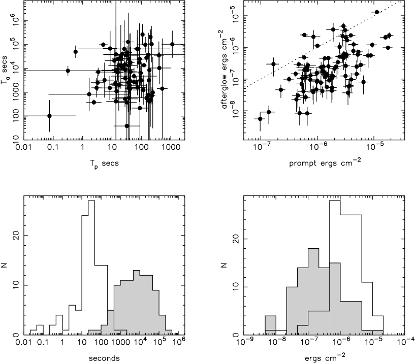
Figure 3: Top left: The afterglow duration $T_{a}$ vs. the prompt duration $T_{p}$ plotted for all objects in which the 2nd component dominates the prompt component at late times. Top right: The afterglow fluence calculated by integrating the 2nd component in the XRT band 0.3-10 keV vs. the prompt fluence calculated from the BAT $T_{90}$ flux 15-150 keV plus the XRT flux 0.3-10 keV in the initial decay ($fl_{dec})$. The dotted line indicates where the prompt and afterglow fluences are equal. Bottom left: Frequency distributions of $T_{p}$ (open histogram) and $T_{a}$ (shaded histogram). Bottom right: Frequency distributions of prompt fluence (open histogram) and afterglow fluence (shaded histogram).

Fig. 3 shows the distribution of $T_{a}$ vs. $T_{p}$ for those objects with two component fits. There is no correlation between these times. The frequency distributions of these times are shown in the bottom left panel. The same figure shows the distribution of afterglow fluence (the total fluence from the afterglow component) vs. the prompt fluence calculated as the sum of the $T_{90}$ fluence seen by the BAT and the fluence from the initial decay $fl_{dec}$ calculated from the XRT flux using the equation above. The dotted line indicates those objects for which the afterglow fluence is equal to the prompt fluence. There are a few objects on or just above this line while the rest are well below. There is a general trend that high prompt fluence leads to high afterglow fluence, as might be expected, but the scatter about this trend is large. This confirms the result from our earlier analysis (O’Brien et al. 2006) but for a larger sample. The frequency distributions of the fluences are shown in the lower right panel of Fig. 3.

3 Spectral evolution

Spectral fitting with XSPEC (Arnaud 1996) version 11.3.2 was used to determine the spectral index in the prompt phase ($\beta_{p}$, from the BAT data), the prompt decay ($\beta_{pd}$ from the XRT data), on the plateau ($\beta_{a}$, XRT data) and in the final decay ($\beta_{ad}$, XRT data) for $t>T_{a}$. In some cases the coverage was poor and/or the count rate low so it was not possible to separate $\beta_{pd}$ and $\beta_{a}$ or $\beta_{a}$ and $\beta_{ad}$. For the weakest bursts it was only possible to derive $\beta_{p}$ and one spectral index from the XRT, $\beta_{pd}$. When fitting late time spectra the absorption was fixed to the early time fitted values (both Galactic and intrinsic components) so that errors on the late time spectral indices were minimised. Table 3 lists these spectral indices for all the GRBs in the sample. The $\pm$ ranges quoted are at 90% confidence. The decay fit type D is also listed. When D=3 there is no 2nd component and hence no plateau. However, for some of these afterglows late time XRT data are available and a late spectral index could be derived independently from $\beta_{pd}$. These late spectral indicies are listed in the $\beta_{ad}$ column.

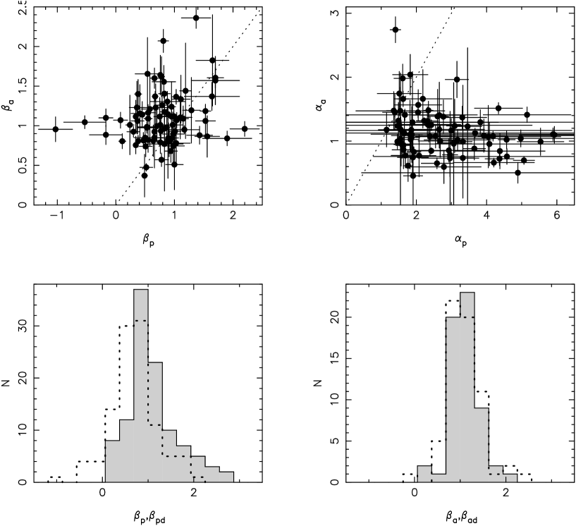
Figure 4: Top left: Comparison of the spectral indices $\beta_{a}$ (2nd, afterglow component) with $\beta_{p}$ (prompt BAT). Top right: Comparison of the decay index for the 2nd component, $\alpha_{a}$ with the prompt component, $\alpha_{p}$ for decays type $D=1$. The dotted lines indicate equality in both panels. Bottom left: Frequency distributions of the prompt component spectral indices, $\beta_{p}$ (dotted histogram) and $\beta_{pd}$ (shaded histogram). Bottom right: Frequency distributions of the afterglow component spectral indices, $\beta_{a}$ (dotted histogram) and $\beta_{ad}$ (shaded histogram).

Fig. 4 shows the distribution of the afterglow plateau spectral index $\beta_{a}$ vs. the prompt (BAT over $T_{90}$) spectral index $\beta_{p}$. The range of indices from the prompt emission is large, $-1.0$ to $2.2$ while the afterglow range is smaller, 0.4 to 2.3. Those objects for which the prompt emission is especially soft ($\beta_{p}>1.8$) or hard ($\beta_{p}<0.1$) evolve to produce an afterglow in the narrow range $0.7<\beta_{a}<1.2$. The frequency distributions of all the spectral indices are shown in bottom panels of Fig. 4. The same figure shows the distribution of $\alpha_{a}$ vs. $\alpha_{p}$ for decays $D=1$. Again, there is no correlation but the range of decay indices for the prompt component is large, 1.0 to 6.0, while the range for the 2nd afterglow component is much smaller, 0.5 to 2.0 with one object at $\alpha_{a}=2.7$. Note, there are 4 decays with $\alpha_{a}>3$ in Table 1 but these are all type $D=2$ marked^∗. In the majority of objects $\alpha_{a}\leq\alpha_{p}$.

4 The expected coupling between $\alpha$ and $\beta$ in the afterglow decay

The standard fireball model predicts that there should be a simple coupling between the temporal decay index in the final afterglow, $\alpha_{a}$, and the spectral index in the final afterglow, $\beta_{ad}$ (Sari, Piran & Narayan 1998). The exact form of the relationship depends on the density profile of the surrounding circum-stellar medium (CSM) and whether the decay is observed before or after a jet break (e.g. Panaitescu & Kumar 2002); because the spectrum is being red-shifted as the jet is slowed down by the CSM and after a jet break the peak flux of the observed synchrotron spectrum is also decaying with time. The top left panel of Fig. 5 shows the temporal decay index of the afterglow component, $\alpha_{a}$, vs. $\beta_{ad}$ the spectral index in the final decay for those objects where $t_{max}>T_{a}$ and for which we have a significant measurement of $\beta_{ad}$ at $t>T_{a}$. There is no correlation between $\alpha$ and $\beta$ and if there is any trend at all it is that some of the faster decays (large $\alpha$) occur for the smaller $\beta$ values. The lower band shown indicates the region of a pre-jet break coupling predicted by the model and the upper band the region expected post-jet break. In each case the lower edge of the band corresponds to the model in which the X-ray frequency is below the cooling break frequency and the CSM density is constant. The upper edge corresponds to the X-ray frequency above the cooling break frequency and a wind density $\propto r^{-2}$. Of the 70 objects plotted, 36 lie below the expectations of the standard model in the bottom right of the plot. For 17 the upper limit of the 90% confidence region in $\beta-\alpha$ doesn’t intersect the pre-jet break band. So for $\approx 50\%$ of GRBs the spectral index of the afterglow is too large to produce the observed temporal decay index. This can only occur under the model if there is significant energy injection such that the peak of the spectrum (or normalisation) is boosted fast enough to counteract the drop expected from the change in red-shift as the outflow slows down. It was pointed out by Nousek et al. (2006) that the spectrum and decay of the plateau phase of several Swift GRBs was inconsistent with the expectations of the model and that energy injection during this phase was a possible explanation. The current analysis shows that the same is also true for many objects during the subsequent decay phase, after the plateau. The lower left-hand panel of Fig. 5 shows $\alpha_{a}-(3/2)\beta_{ad}$ plotted as a function of $T_{a}$. This function will be zero for pre-jet break afterglows under the standard model (with uniform CSM and the X-ray frequency below the cooling frequency) and negative for afterglows with a value of $\alpha_{a}$ which is too small compared with the $\beta_{ad}$. The horizontal dashed line is the pre-jet break expectation if the X-ray frequency is above the cooling frequency. Consideration of GRB efficiencies (Zhang et al. 2006) indicates that more than 60% of afterglows in the sample described by O’Brien et al (2006) do lie above the cooling break. If this is the case for the present, larger, sample a significant fraction of the GRBs plotted as dots (pre-jet break) are also outside expectation. The figure also indicates that there is no correlation of this function with the time at which the final decay starts, so if energy injection is the explanation it is occurring at large times, $>10^{5}$ seconds as well as much earlier times. Of the remaining $\sim 50\%$ of objects plotted on the top left-panel of Fig. 5, 26 lie within the pre-jet break band while 8 lie above this close to or within the post-jet break region. It is conceivable that some of the anomalously large $\beta$ values could be associated with the fitted absorption (both Galactic and intrinsic). We checked this possibility but found no correlation between the position of an afterglow on the $\beta-\alpha$ plane and the fitted $N_{H}$.

The top right-hand panel of Fig. 5 shows the change in spectral index into the final decay from the plateau, $\Delta\beta=\beta_{ad}-\beta_{a}$ plotted vs. the plateau spectral index $\beta_{a}$. Here there is a trend. If $\beta_{a}$ is small then $\Delta\beta>0$ and the afterglow gets softer in the final decay. If $\beta_{a}$ is large then $\Delta\beta<0$ and the final decay is harder. The scatter of index $\beta_{ad}$ is smaller in the final decay, being confined to the range 0.0 to 2.2 as indicated on the top left plot. The gradual narrowing of the spectral index range as the afterglows develop can also be seen in the frequency distributions shown in the lower panels of Fig. 4. One object, GRB060218, has an anomously large final spectral index, $\beta_{ad}=3$, but this GRB was very peculiar in many respects, in particular for having a significant thermal component in the early X-ray spectrum, Campana et al. (2006). No $\beta_{a}$ was derived for this afterglow because the plateau is largely obscured by unusual, persistent, prompt emission. The trend in the change in spectral index from the plateau into the power law decay is independent of the position in the $\beta-\alpha$ plane occupied by the final decay.

The above discussion has considered those objects with a 2nd afterglow component that dominates in the later regions of the X-ray light curve (D=1). 22 of the X-ray decays required no 2nd component (D=3) or have a 2nd component which produced a hump in the decay but faded towards the end (D=2). In these cases the initial decay of the prompt component dominates at late times. The bottom right-hand panel of Fig. 5 shows the correlation between the late temporal decay index ($\alpha_{p}$) and spectral index of these objects. The behaviour is very similar to objects (D=1) shown in the top left panel. There is no obvious correlation and 8 of the 21 object fall below the expected correlation in the bottom right. Also plotted in this panel are the $\beta_{ad}$,$\alpha_{b}$ values for the late breaks listed in Table 2. Five of these lie within the pre-jet break band but three, GRB050814, GRB060105 and GRB060607A, are within the post-jet break region although the errors on the decay index after the late break temporal break, $\alpha_{b}$, are rather large. The complete X-ray light curve for GRB050814 containing the late temporal break is shown in the upper right panel of Fig. 8. Further analysis of GRB060105 is provided by Godet et al. (2006a). GRB06067A is similar to GRB060105.

5 Isotropic energy of the prompt and afterglow components

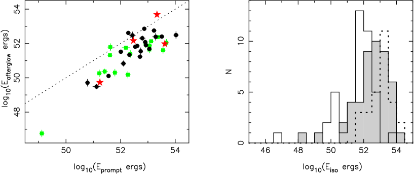
Figure 6: Left: The isotropic afterglow energy vs. the isotropic prompt energy. Symbols indicate the position of the afterglow in the $\beta$-$\alpha$ plane as in Fig. 5. The dotted line indicates equality between the prompt and afterglow energies. Right: The distribution of isotropic energies. Filled histogram $E_{prompt}$ and solid line histogram $E_{afterglow}$. The dotted histogram is the distribution of $E_{iso}$ for GRBs observed before the Swift era as tabulated by Frail et al. (2001), Bloom et al. (2003) and Ghirlanda et al. (2004).

Fig. 3 shows the correlation between the fluences in the prompt component (including the BAT $T_{90}$ 15 to 150 keV and the initial decay in the XRT 0.3 to 10 keV) and the afterglow component. For those bursts for which we have a redshift (z values listed in Table 3) these fluences can be used to estimate the equivalent isotropic energy. We assumed a cosmology with $H_{o}=71$ km s^-1 Mpc^-1, $\Lambda=0.27$ and $\Omega=0.73$ and calculated $E_{iso}$ over an energy band of 1 to 10000 keV in the rest frame applying a k-band correction independently for the BAT and XRT data. For many objects we don’t have a measured value of the peak energy in the spectrum. In such cases we assumed $E_{peak}=116$ keV (the median value for Swift bursts) and a spectral index of $\beta=2.3$ for $E>E_{peak}$. The mean $E_{peak}$ for BATSE (pre-Swift) bursts was 235 keV (170-340 keV 90% range) (Kaneko et al. 2006) which is significantly larger than for Swift bursts, mean 138 keV, median 116 keV. However the mean redshift for Swift bursts considered here is 2.46 while for pre-Swift bursts it is $\approx 1.52$ so we expect the mean/median $E_{peak}$ for Swift bursts to be $\sim 0.6$ the BATSE value. The mean value for the spectral index above $E_{peak}$ for BATSE bursts was 2.3 (Kaneko et al. 2006). Fig. 6 shows the equivalent isotropic energy for the two components. The symbols used are the same as in Fig. 5. It is clear that the total energy in the afterglow is not correlated with the position of the final afterglow in the $\beta$-$\alpha$ plane. Note that the correlation between the equivalent isotropic energy components evident in Fig. 6 is real but not particularly significant since it arises from applying the measured redshift in both axes. In many objects the total energy seen in X-rays from the afterglow is significant compared with the $\gamma$ and X-ray energy seen from the prompt component. The dotted histogram in the right panel shows the distribution of $E_{iso}$ values for GRBs observed by instruments pre-Swift taken from the tabulations in Frail et al. (2001), Bloom et al. (2003) and Ghirlanda et al. (2004). The maximum isotropic energy in the $Swift$ sample is similar to the maximum seen previously, $\approx 10^{54}$ ergs, but the distribution of energies seen by $Swift$ is broader, has a lower mean and extends to a lower limit of $\approx 10^{47}$ ergs.

6 Temporal breaks

The visibility of the 2nd component used here to fit the X-ray decay curves depends on the relative brightness of the prompt emission decay compared with the afterglow plateau and the times $T_{p}$ and $T_{a}$. If $T_{a}$ is not long after $T_{p}$ then the end of the plateau phase is not visible, as is the case for the decay shown at the top left of Fig. 2. However, for 64 of the 91 GRBs which required 2 components in the fit the end of the plateau is visible, as is the case for the exemplar GRB shown at the top right of Fig. 2. In such cases the plateau gets slowly steeper towards the end of the exponential phase and eventually relaxes to a power law. There is often no definitive or sharp break but the time $T_{a}$ is a robust measure of where this transition occurs, taking into account all the data available. Thus, the fitting provides 91 afterglow break times, $T_{a}$, from a total of 107 objects.

In some cases it may be that any jet break time associated with the edge of a putative jet becoming visible occurs at or before $T_{a}$. In such decays we expect the subsequent afterglow to lie somewhere in the top left of the $\beta-\alpha$ plane shown in Fig. 5 and the 8 candidates for such cases are shown as star symbols on this figure. Note that the error bars shown in Fig. 5 are at 90% confidence and there is one object lying in the lower pre-jet break band which is also consistent with the upper post-jet break band. The time $T_{a}$ for these GRBs is not a pure jet break time since in all cases the $T_{a}$ marks the end of the plateau phase which does not behave as a pre-jet afterglow (e.g. Nousek et al. 2006). The only evidence for a jet break having occurred in these 8 candidates is that the $\alpha$ and $\beta$ values of the subsequent decay have the right relationship for a post-jet break afterglow. Since 50% of afterglows don’t agree with the expected alpha-beta value, including the pre-jet break values, the argument in favour of jet breaks in these cases is weak. However, $T_{a}$ is a reasonable estimate of where any jet break may have occurred. Details of these 8 potential jet breaks are given at the top of Table 4.

As discussed above, an additional 8 GRBs required a late break to fit the data as illustrated at the bottom of Fig. 2. The positions of the final afterglows in the $\beta-\alpha$ plane for these GRBs are shown in the bottom right of Fig. 5 (plotted as triangles). Only 4 of these objects are good candidates for jet breaks and these are listed at the bottom of Table 4 and illustrated in Fig. 8. The jet break time ranges plotted were estimated using the Ghirlanda relation assuming $E_{peak}=116\pm 50$ keV (there are no measured values of $E_{peak}$ for these bursts). For GRB060607A, in the bottom right panel, the late break occurs slighly earlier the allowed band indicating that, for this break to be consistent with Ghirlanda, the $E_{peak}$ should be $<66$ keV. So, in summary, out of 72 afterglow breaks identified by the fitting procedure only 12 are followed by an afterglow which is consistent with post-jet break conditions and only 4 of these are isolated breaks independent of the end of the plateau phase. The remaining 60 have slow X-ray decays (low $\alpha$) and/or soft X-ray spectra (high $\beta$).

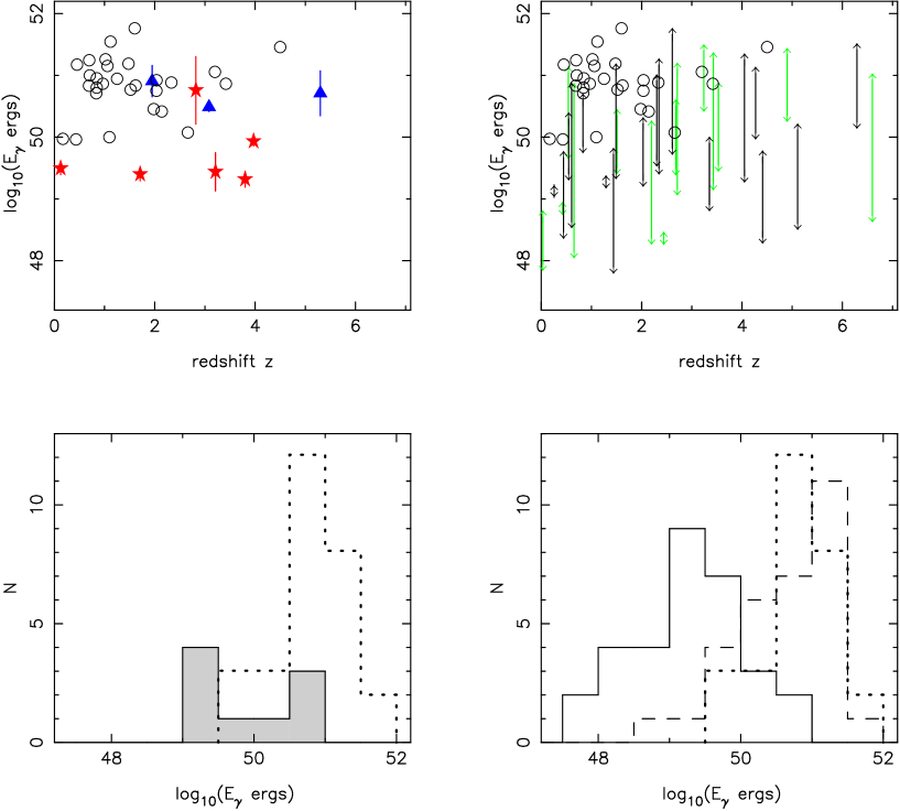
Figure 7: The jet energy $E_{\gamma}$ calculated using equation 1. Top left: The stars and triangles correspond to the jet break times listed in Table 4 (symbols as Fig. 5). The open circles are the values obtained using the $t_{j}$ and $E_{iso}$ tabulated by Frail et al. (2001), Bloom et al. (2003) and Ghirlanda et al. (2004). Top right: Ranges of $E_{\gamma}$ excluded by the X-ray decays without breaks, $t>T_{a}$. The lower points are from $T_{a}$ and upper from $t_{max}$ (the end of the light curve). Bottom left: The filled histogram shows the distribution of $E_{\gamma}$ for the breaks listed in Table 4. The dotted histogram is the Frail-Bloom-Ghirlanda sample.

The interest in jet breaks stems from Equation 1 which can provide an estimate of the jet angle $\theta_{j}$ and hence the collimation-corrected energy $E_{\gamma}$. For calculation of all the subsequent $E_{\gamma}$ values considered below we have assumed $n\eta_{\gamma}=0.6$ (or equivalently $n=3$ cm^-3 and $\eta_{\gamma}=0.2$). $\eta_{\gamma}=0.2$ has been widely assumed in pre-Swift analysis although recent work using Swift data (Zhang et al. 2006) indicates that the efficiency can be determined with more accuracy. However, since $E_{\gamma}\propto(n\eta_{\gamma})^{1/4}$ the resulting collimated energy is fairly insensitive to these parameters. For 9 of the objects in Table 4 we have redshifts and can estimate $E_{\gamma}$ using the jet break time. These are shown in Fig. 7. The symbols are the same as in Fig. 5. Also shown are the values derived for pre-Swift GRBs using the tabulations in Frail et al. (2001), Bloom et al. (2003) and Ghirlanda et al. (2004). For 31 others we have redshifts (as listed in Table 3) but there is no break between $T_{a}$ and the last data point at $t_{max}$. For these decays we can calculate a range of $E_{\gamma}$ which is excluded by the decay. These ranges are plotted in the top right-hand panel of Fig. 7 with the energy corresponding to $T_{a}$ at the lower end of each range and to $t_{max}$ at the upper end. For many afterglows the excluded range of $E_{\gamma}$ covers a substantial fraction of the pre-Swift distribution. The lower panels of the same figure shows the respective frequency distributions. The 3 objects with measured late breaks are in good agreement with the peak of the pre-Swift $E_{\gamma}$ distribution published by Frail and Bloom. Of the remaining 6 objects in which $T_{a}$ has been identified with a possible jet break 2 lie within the lower wing of the pre-Swift distribution and 4 lie below. The distribution of $E_{\gamma}$ values derived from the remaining $T_{a}$ values is similar in shape to the pre-Swift distribution calculated using optically observed jet break times but is offset to lower energies by a factor of $\approx 34$. This corresponds to an average jet break time which is a factor $\approx 110$ smaller or a jet angle which is a factor $\approx 10.5$ smaller. The times $T_{a}$ derived from the X-ray decay curves are, on average, a factor of $\approx 80$ smaller than the optical jet break times observed for pre-Swift GRBs. The peak of the distribution of $E_{\gamma}$ values calculated from $t_{max}$ is significantly higher than the pre-Swift distribution because many of the X-ray decays extend to later times without a temporal break.

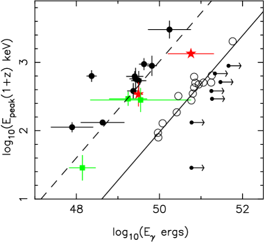
Figure 9: The open circles and solid line are the Ghirlanda relation. The points with error bars are Swift GRBs for which values of $E_{\gamma}$ were derived using the Ghirlanda relation assuming $t_{j}=T_{a}$. The symbols plotted are the same as in Fig. 5. The dashed line is a fit to the Swift sample assuming the slope is fixed at 0.706, the best fit value from Ghirlanda et al. (2004). The lower limits of energy shown were derived using the latest observed time as $t_{j}$ for GRBs with lasting afterglow decays which show no break (the light curves plotted in Fig. 10). $E_{peak}$ values used here and for Figures 8 and 10 were taken from Cummings et al. (2005), Crew et al. (2005), Golenetskii et al. (2005, 2006) or they were derived from spectal fitting of the BAT data.

$T_{a}$ is the only measure we have (or require) to specify the timescale of the 2nd afterglow component. It is clear from the discussion above that, in almost all cases, this does not represent a jet break time. However, given that it is the only time extracted from the X-ray data it may be related to the previously observed optical jet break times. There are 14 GRBs for which we have a $T_{a}$ value, a redshift and a measurement of the peak energy of the $\gamma$-ray spectrum, $E_{peak}$. For these objects we can construct a Ghirlanda type correlation between the peak energy in the rest frame $E_{peak}(z+1)$ and the collimated beam energy $E_{\gamma}$ calculated assuming $t_{j}=T_{a}$. This is shown alongside the conventional Ghirlanda relation in Fig. 9. The X-ray measurements show a similar behaviour, not as statistically significant as the optical version but with about the same gradient and an offset in $E_{\gamma}$ by a factor of $\approx 26$. For these cases the X-ray break times, $T_{a}$, are a factor of $\approx 90$ less than pre-Swift optical break times. Unfortunately none of the GRBs with potential X-ray jet breaks identified and plotted in Fig. 8 has a measured $E_{peak}$ value so these can’t be included on Fig. 9. However, we can calculate lower limits to $E_{\gamma}$, assuming $t_{j}=t_{max}$, for those decays without a late break but with an $E_{peak}$ and redshift measurement. These are included on Fig. 9. They all lie to the right of the Ghirlanda correlation. There is currently one afterglow observed by Swift, GRB050820A, for which we have derived a time $T_{a}$ and the optical coverage extends to $\sim 100\times T_{a}$ (Cenko et al. 2006). In this case the optical decay does appear to have a break at about the expected time, $t_{j}\approx 100\times T_{a}$. The Ghirlanda correlation was originally formulated by considering the jet model and the collimated jet energy however, the correlation derived here, using $T_{a}$ from the X-ray afterglows, has more in common with the model independent analysis described by Liang & Zhang (2005). The Liang-Zhang $E_{iso}-E_{peak}-t_{b,opt}$ correlation may well be related to the $E_{iso}-E_{peak}-T_{a}$ correlation plotted in Fig. 9.

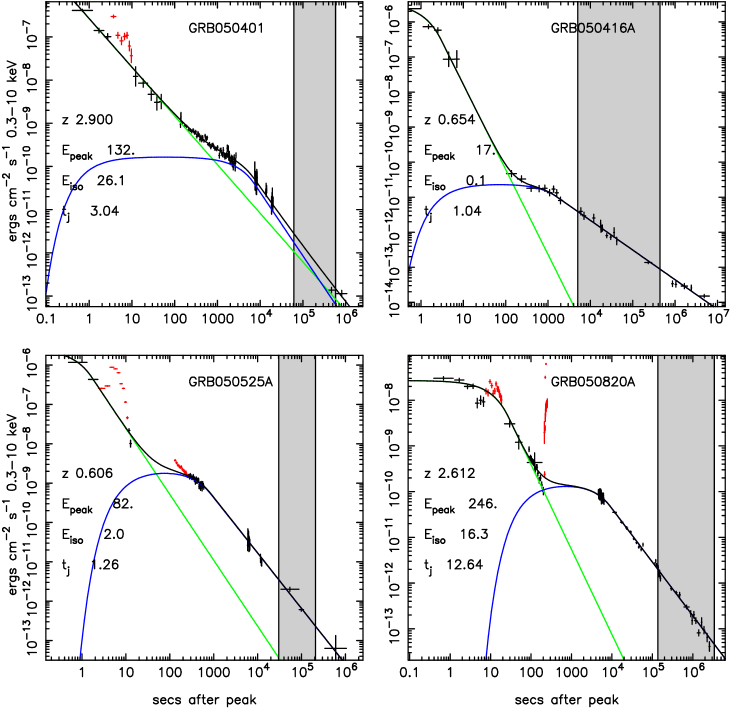
Figure 10: X-ray decays in which a predicted jet break is absent. $E_{peak}$ listed in keV, $E_{iso}$ in 10⁵² ergs and $t_{j}$ in days. The shaded area indicates the expected range for $t_{j}$. For GRB060510B and GRB060729 there is no measured $E_{peak}$ value so $116\pm 50$ keV has been assumed (see Section 5).

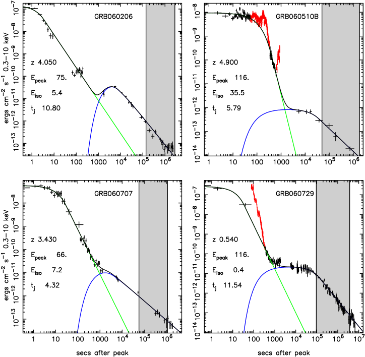
Figure 10: cont.

As a natural consequence of the above discussion, and following Sato et al. (2006), we can adopt a different approach and look for X-ray decays in which a predicted jet break is absent. Apart from GRB050401 (or XRF050401, Mangano et al. 2006, Sakamoto et al. 2006), GRB050416A and GRB050525A already considered by Sato et al. (2006) there are 5 other X-ray decays monitored by Swift which come under this category. Light curves for all 8 are shown in Fig. 10. In each case the expected range for the jet break time, $t_{j}$, is shown as the shaded area. Each decay was followed for at least a factor of 100 times longer than $T_{a}$ without any indication of a break in the temporal decay index. For GRB060206 there is some indication that the X-ray light curve is flattening for $t>10^{6}$ seconds. This is probably due to systematic errors in the background subtraction when the afterglow is very faint and/or contamination by a faint, nearby, background object. GRB050525A, GRB050820A, GRB060510B and GRB060729 are cases where there is a large flare at the end of the prompt phase and the late BAT and/or early XRT data are not well fitted by the prompt function. However, the plateau and subsequent power law decay are well represented by the afterglow component in all cases. The late afterglow of GRB060729 has currently been monitored for 77 days without any indication of a break.

Optical data are available for 5 of the final power law decays of these afterglows; GRB050525A (Blustin et al. 2006), GRB050820A (Aslan et al. 2006, Cenko et al. 2006), GRB060206 (Stanek et al. 2006, Monfardini et al. 2006), GRB060707 (de Ugarte Postigo et al. 2006, Jakobsson et al. 2006) and GRB060729 (Grupe et al. 2006). Optical jet breaks are not seen in any of these afterglows although the decays of GRB050525A, GRB060206 do gradually steepen at late times and there is a one final late measurement at $\sim 3\times 10^{6}$ seconds for GRB050820A which indicates that the optical decay has turned down (HST data presented in Cenko et al. 2006 as already mentioned above). We have fitted these optical afterglows with a simple power law over the period contemporary with the final X-ray decay ($t>T_{a}$) and the results are shown in Table 5. For 4 afterglows the X-ray and optical decay indices are consistent. For GRB050820A the optical index is formally significantly lower than the X-ray index but there is structure in the optical decay curve which is not well modelled by a single power law fit. For all 5 the X-ray and optical decays are remarkably similar and shallow with decay indices in the range 0.75-1.5 and they all have $\alpha,\beta$ reasonably consistent with a pre-jet break afterglow.

Two other objects, GRB050822 (Godet et al. 2006b) and GRB060218 (Campana et al. 2006) also have Swift X-ray light curves with extended coverage of a long power law decay without a break. Both these objects have soft spectra and are more reasonably considered as XRFs with $E_{peak}<25$ keV. For GRB060218 we have a measured redshift of 0.0333 (Mirabal & Halpern 2006). Adopting a range of $E_{peak}$ values consistent with an XRF (and a range of redshift values for GRB050822) it can be shown that a jet break should have been seen at some point in the X-ray light-curves of both these objects but none was observed (Godet et al. 2006b). For GRB060218 radio observations have shown that the fireball was probably isotropic (Soderberg et al. 2006) and similarly, in the cases of GRB050416A and GRB050822, it is possible that the jet opening angle was wide ($>20$ degrees). For the XRFs a large opening angle and consequent absence of a jet break is not unreasonable because $E_{iso}$ is typically rather low. There are also 9 further GRBs (050318, 050603, 050802, 060108, 060115, 060418, 060502A, 060614 and 060714) for which we can predict a range of jet break times and no break is seen. For these objects the lowest predicted $t_{j}$ is well before the last observed time but the upper limit on $t_{j}$ is after the last observed time so we cannot rule out the possibility that a break occurred too late (and too faint) to be seen by the Swift XRT. There is a suggestion of a late break for GRB060614 but inclusion of such a break is not statistically significant under the current analysis.

An important property of a jet break is that it should be achromatic, occurring across the spectrum with the same temporal profile. Panaitescu et al. (2006) show that temporal breaks for 6 GRBs seen by the Swift XRT are not present in optical data which span the same period of time. For 5 of these, GRB050802, GRB050922C, GRB050319, GRB050607 and GRB050713A the break in the X-ray decay is fitted as $T_{a}$ in the analysis presented above. Therefore for these objects optical data do not follow the X-ray profile modelled by the 2nd afterglow component and the observed X-ray break is unlikely to be a jet break. The remaining object, GRB050401, is fitted using 2 components but the 2nd component appears as a hump in the X-ray decay and the 1st component has a slow decay, $\alpha_{p}=1.12\pm 0.05$, that dominates near the end. So in this case the optical data seem to follow the behaviour of the power law decay of the 1st prompt component and not the 2nd component. Similar behaviour is exhibited by GRB060210 which has the same relationship between the 1st and 2nd X-ray component, $\alpha_{p}=1.0\pm 0.07$, and the available optical data (Stanek et al. 2006) follow the decay of the 1st component. Conversely, there are examples of GRB decays for which the X-ray and optical profiles do follow a similar pattern. Optical data for GRB060206 (Stanek et al. 2006) have a profile which closely follows the 2nd component of the X-rays. Stanek et al. argue that for this GRB there is a break which can be seen simultaneously in optical and X-rays but the present analysis finds no such X-ray break. Instead there is a gentle curvature in the X-ray (and optical) decay which is modelled by the slow transition from exponential to power law in the profile of the 2nd afterglow component. GRB050525A is another example in which curvature in the later stages of the X-ray and optical can be modelled as a break (Blustin et al. 2006). The present analysis finds no such break in the later stages of the X-ray decay of this burst either.

7 Conclusions

The X-ray decay curves of 107 GRBs observed by Swift have been fitted in a systematic way using the simple functional form given by Equation 2. They all require a prompt component with parameters $T_{p}$, $F_{p}$ and $\alpha_{p}$ and 85 require a 2nd afterglow component with parameters $T_{a}$, $F_{a}$ and $\alpha_{a}$. The parameters and associated confidence limits are all listed in Table 1. $T_{p}$ is similar to the familiar $T_{90}$ burst duration as discussed by O’Brien et al. (2006). $\alpha_{p}$ is a prompt parameter which was unavailable before the Swift era and indicates how fast the prompt emission is decaying as also discussed by O’Brien et al. (2006). The product $T_{p}F_{p}$ combined with $\alpha_{p}$ is a measure of the prompt fluence (see Equations 3 and 4). $\alpha_{p}$ also determines the distribution of energy. If $\alpha_{p}<1.446$ then more energy is emitted for $t>T_{p}$ during the prompt power law decay phase and if $\alpha_{p}>1.446$ more energy is emitted during the prompt exponential phase $t<T_{p}$. $T_{a}$ is the time when the final afterglow power law decay starts, $\alpha_{a}$ is the index of this final decay and also controls the curvature of the proceeding plateau phase and the product $T_{a}F_{a}$ along with $\alpha_{a}$ combine to give a fluence of the afterglow component (sum of Equations 3 and 4 replacing subscripts $p$ with $a$). $\alpha_{a}$ controls the distribution of energy in the 2nd functional component in the same way as $\alpha_{p}$ controls this distribution in the prompt component, as described above. In addition, spectral fitting has provided $\gamma$ and X-ray spectral indices over the phases of these functional fits as listed in Table 3. The combination of Tables 1 and 3 provides a rich data base for comparison with theoretical models.

The functional form used for the fits (Equation 2) is empirical rather than based on a physical model and it doesn’t accomodate flares. However, the exponential rise at time $t_{c}$ and transition from exponential to power law at $T_{c}$ are reminiscent of the theoretical discussion of the development of an afterglow given by Sari (1997). Employing exponentials, rather than power law sections with breaks, provides a curvature which neatly fits the data and produces a remarkably good representation of the underlying X-ray decay profile with the minimum number of parameters. In any physical model the number of parameters that could influence the shape of the X-ray light curves is large but some combination or subset of these are likely to be represented by the values tabulated here.

Most ($\approx 80\%$) GRBs have a 2nd afterglow component which dominates at later times and this is probably the expected emission from the external shock. For these objects the prompt and afterglow components appear to be physically distinct. Bursts marked^∗ in Table 1 (or D=2 in Table 3) have 2 component fits but the 1st prompt component dominates at later times. For these GRBs and those which only require 1 component in the fit (D=3 in Table 3) it is not clear where such an early prompt decay component comes from. It could be the external shock but if this is the case then the external shock is developing very early ($t<T_{p}$) and the prompt decay emission from this shock is distinct from the more common external shock emission seen in the 2nd component. In GRBs marked^∗ (D=2 in Table 3) both these external shock components are seen. For these objects it is not so obvious that the prompt and afterglow components fitted map directly to two physical entities. The hump in the decay curve could be a signature of the presence of different outflow structures (e.g. Eichler & Granot 2006) or a universal structured jet (e.g. Mészáros, Rees & Wijers 1998). Two of the GRBs, GRB051210 and GRB051221B, fitted by just one component (D=3 in Table 3) could be “naked GRBs” for which there is no external shock and the prompt decay arises solely from high latitude emission (Kumar & Panaitescu 2000). Such GRBs are expected to have $\alpha_{p}-\beta_{pd}=2$. This difference is $1.81\pm 0.2$ for GRB051210 and $1.73\pm 1.0$ for GRB051221B consistent with a high latitude interpretation. Neither of these bursts were detected after the 1st orbit post trigger. GRB051210 has an upper limit from the 2nd orbit consistent with the steep power law decay. For GRB051221B upper limits were obtained from the 2nd orbit and much later, $t=4.6\times 10^{5}$ seconds, both again consistent with a steep prompt decay and no afterglow or plateau. The remaining 14 single component prompt decays were not steep with mean $\alpha_{p}=1.35\pm 0.22$ and significantly lower $\alpha_{p}-\beta_{pd}$ values with a mean of $0.6\pm 0.4$. Although a rise time, $t_{a}$, was included in the afterglow function fit in most cases it was set at some arbitarily early time when any increase in this component would be obscured by the prompt emission. Thus, the functional fits provide very little evidence for any observational signature of the “onset” of the afterglow or a rising afterglow component predicted in some off-axis models (Eichler & Granot 2006). The afterglow could be established very early. Since the outflow is presumed to be moving close to the speed of light there may be very little time delay between prompt emission and emission from the external shock when the outflow begins to decelerate.

There is no tight correlation between the prompt component parameters and the afterglow component parameters. There is a trend that the larger the prompt fluence the larger the afterglow fluence, as might be expected, and the afterglow energy is usually considerably less than the prompt energy. In some cases the afterglow energy is about equal to the prompt but we never see afterglows which are much more energetic than the prompt emission; see Figures 3 and 6.

Almost all of the X-ray afterglows end up in the same region of the $\beta-\alpha$ plane, $0.5<\beta<2$ and $0.4<\alpha<2$, independent of the other parameters. However, $\approx 50\%$ of these afterglows are in the bottom right of the $\beta-\alpha$ plane with high $\beta$ and low $\alpha$, values not predicted by the standard fireball model. This may be due to persistent long lasting energy injection but this seems unlikely in such a high percentage of objects and at such late times. Furthermore the trend expected from the model, that high $\beta$ values should give high $\alpha$ values and vice versa, is not seen at any level of significance. If this is because of energy injection this energy injection is occurring in just the right number of afterglows and at just the right level such that the expected $\beta-\alpha$ coupling is hidden or masked. If, for example, energy injection were always present at some fixed level all afterglows would be shifted to lower $\alpha$ values but any correlation would be preserved. In fact, if energy injection occurred preferentially at late times post-jet break afterglows would be shifted to smaller $\alpha$ values but pre-jet break afterglows would not be altered and the overall correlation including both pre and post jet break afterglows might be tightened. The curvature or break which marks the end of the afterglow plateau phase at time $T_{a}$ is often accompanied by a small spectral change such that soft afterglows become somewhat harder and hard afterglows become softer bringing the final afterglow spectral index into the rather narrow range indicated above.

For the 91 GRBs which require a 2nd afterglow component we derive time $T_{a}$ which marks the end of the plateau and the start of the final decay. For 64 cases we can see this transition/break in the data. Do we see any jet breaks? For 8 GRBs the final temporal decay and spectral index $t>T_{a}$ are consistent with the jet model after a jet break has occurred but for 6 of these objects for which we have a redshift the $E_{\gamma}$ values are low compared with the distribution derived from consideration of optical jet breaks and the implied jet angles are small. 8 X-ray decays have a late break, $T_{b}>T_{a}$, and 4 of these have final $\alpha$ and $\beta$ values consistent with a post jet break afterglow. 3 of these have redshifts and $E_{\gamma}$ values which are in accord with the pre-Swift distribution. On the other hand there are 11 decays with long-lasting coverage, $t>T_{a}$, in which a jet break predicted using the Ghirlanda relation is definitely not seen and there are a further 9 objects in which a break is not seen but it may have occurred at a rather late time beyond the coverage provided by the sensitivity limit of the Swift XRT. 13 decays (in the top right and bottom left panels of Fig. 5) have been identified as lying in the post jet-break region of the $\beta-\alpha$ plane (star symbols). For such decays the electron energy distribution index is expected to be equal to the decay index. Two of these decays, GRB060421 and GRB060526, have decay indices $<1.6$ (see Table 4), probably too low to be the same as the electron index.

There are currently $\sim 10$ afterglows for which there are both X-ray and optical data available during the X-ray plateau and into the final decay (and there are a few more objects for which such data will soon be publically available). The X-ray and optical often follow a similar trend but temporal breaks which are seen in one band are not always seen in the other. This is probably because the end of the plateau and start of the final power law is marked by a continuous curvature such that the light curves in both bands are slowly getting steeper. Rather than fitting isolated temporal breaks independently in either band we suggest that simultaneous fitting of a profile as described by Equation 2 in an attempt to find a value for $T_{a}$ which is consistent with both the X-ray and optical data would be more illuminating. Such a joint fit would also provide a best estimate of the fluence ratio between the X-ray and optical bands (or equivalently the X-ray/optical flux ratio).

If we assume that $T_{a}$ is a jet break time $t_{j}$ and calculate $E_{\gamma}$ for those objects with redshifts the distribution of $E_{\gamma}$ which results is very similar to the distribution derived from optical jet breaks but is offset to lower energies by a factor $\approx 34$ implying that any optical jet break should be seen at time $t_{j}\approx 110\times T_{a}$. Furthermore, for those GRBs for which we have an $E_{peak}$ value for the $\gamma$-ray spectrum the peak energy in the rest frame is correlated with the collimated energy estimate $E_{\gamma}$, in the form of a Ghirlanda relation, but with the $E_{\gamma}$ values offset to lower energy by a factor $\approx 26$ which implies that $t_{j}\approx 90\times T_{a}$. It appears that $T_{a}$ extracted from X-ray decays in the present analysis has properties related to $t_{j}$ derived from optical data. Whether this apparent connection is purely statistical in nature or has some deeper significance remains to be seen but it is doubtful that either $T_{a}$ or $t_{j}$ are actually “jet break” times. However, it is likely that the end of the plateau phase, $T_{a}$, does depend on the total energy in the outflow, the collimation angle of the outflow and the density of the CSM and that the $E_{iso}-E_{peak}-T_{a}$ correlation reported here is related to the $E_{iso}-E_{peak}-t_{b,opt}$ relation discussed by Liang & Zhang (2005).

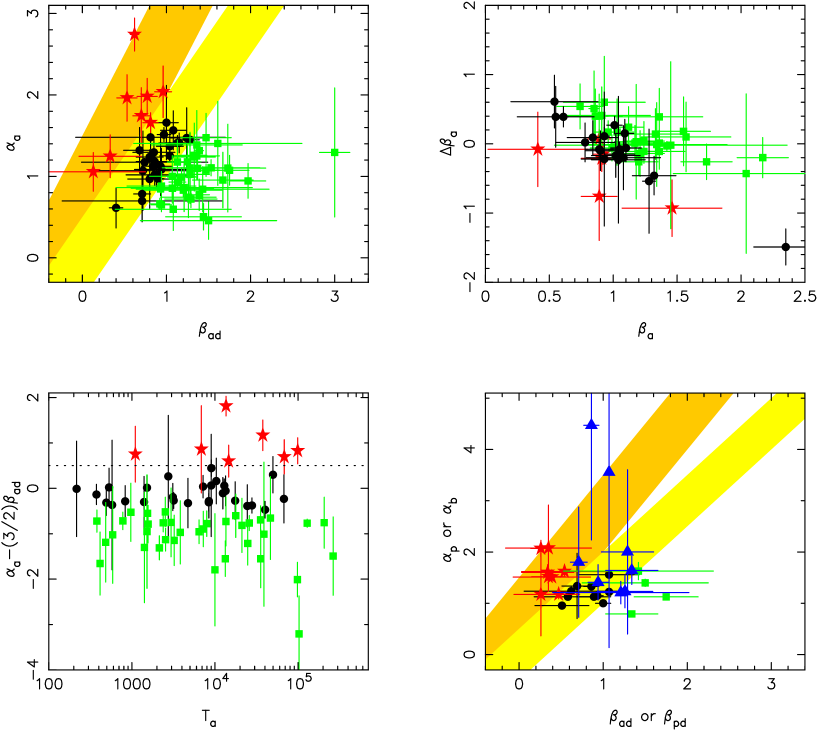
Figure 5: Top left-hand panel: the temporal decay index of the afterglow plotted vs. the spectral decay index in the final afterglow decay. The lower band (yellow) indicates the area expected to be occupied by a pre-jet break afterglow and the upper band (orange) the area post-jet break. GRBs which fall in the pre-jet break region are plotted as circular dots (black), those which fall above this in the post-jet break region are plotted as stars (red) and those below the pre-jet break band are plotted as squares (green). The same symbols are used in the other three panels. Top right-hand panel: change in spectral index $\beta_{ad}-\beta_{a}$ vs. the plateau spectral index $\beta_{a}$. Bottom left-hand panel: $\alpha_{a}-(3/2)\beta_{ad}$ vs. the duration of the afterglow $T_{a}$. This function is expected to be zero for a pre-jet break afterglow in a uniform CSM with the X-ray frequency below the cooling break frequency. The dotted line indicates the zero if the X-ray frequency is above the cooling break frequency. Bottom right-hand panel: the temporal decay index vs. the spectral index for afterglow power law decay in objects which require only one component in the fitting or in which the prompt component dominates at the end of the X-ray light-curve. The $\beta_{ad}$ vs. $\alpha_{b}$ for the late temporal breaks listed in Table 2 are also shown as triangles (blue). The bands shown are the same as for the top left-hand panel.

Bottom right: The dotted histogram is the Frail-Bloom-Ghirlanda sample. The solid line histogram is the distibution derived from $T_{a}$ and the dashed line histogram from $t_{max}$.

Table 1: Best fit parameters for the Swift X-ray decay curves together with upper and lower 90% confidence limits. Times are in seconds and fluxes in ergs cm^-2 s^-1 0.3-10 keV. $t_{p}$ is the prompt peak time with respect to the BAT trigger time used as time zero. ^∗2 component fits in which the 1st prompt component dominates towards the end of the X-ray light curve. ^†These GRBs have less than 50% of $T_{90}$ included in the fitting.

GRB	$t_{p}$	$\log_{10}(T_{p})$	$\log_{10}(F_{p}T_{p})$	$\alpha_{p}$	$\log_{10}(T_{a})$	$\log_{10}(F_{a}T_{a})$	$\alpha_{a}$
050126	$0.89$	$1.95_{\;1.70}^{\;2.26}$	$-6.96_{-8.10}^{-6.86}$	$4.05_{\;3.04}^{\;7.17}$	$2.34_{\;1.34}^{\;5.64}$	$-8.10_{-10.74}^{-6.47}$	$1.07_{\;0.63}^{\;1.61}$
050128	$1.50$	$0.51_{\;0.32}^{\;0.77}$	$-7.02_{-7.11}^{-6.89}$	$1.16_{\;1.02}^{\;1.49}$	$3.40_{\;3.07}^{\;3.73}$	$-6.88_{-7.10}^{-6.79}$	$1.18_{\;0.99}^{\;1.52}$
050219A†	$0.50$	$1.30_{\;0.30}^{\;2.30}$	$-7.07_{-7.12}^{-7.03}$	$1.55_{\;1.49}^{\;1.61}$	$4.49_{\;3.49}^{\;5.81}$	$-7.28_{-8.89}^{-6.03}$	$1.03_{\;0.00}^{\;11.63}$
050315	$2.04$	$1.95_{\;1.89}^{\;2.01}$	$-6.26_{-6.43}^{-6.16}$	$4.37_{\;4.03}^{\;4.84}$	$4.39_{\;4.13}^{\;4.66}$	$-6.94_{-7.07}^{-6.82}$	$0.72_{\;0.63}^{\;0.84}$
050318	$0.00$	$-1.13_{-2.13}^{-1.22}$	$-6.59_{-8.40}^{-4.23}$	$1.39_{\;1.26}^{\;1.96}$	$2.01_{\;1.37}^{\;2.68}$	$-5.99_{-6.30}^{-5.77}$	$1.45_{\;1.22}^{\;1.78}$
050319†	$10.56$	$1.52_{\;1.37}^{\;1.68}$	$-5.87_{-5.94}^{-5.80}$	$2.61_{\;2.37}^{\;2.94}$	$4.67_{\;4.40}^{\;4.93}$	$-6.70_{-6.78}^{-6.61}$	$1.39_{\;1.01}^{\;1.86}$
050401∗	$0.02$	$-0.31_{-1.31}^{\;0.07}$	$-6.54_{-6.61}^{-6.05}$	$1.13_{\;1.09}^{\;1.18}$	$3.87_{\;3.69}^{\;4.11}$	$-6.54_{-6.62}^{-6.48}$	$1.47_{\;1.27}^{\;1.94}$
050406	$0.62$	$1.13_{\;0.73}^{\;1.37}$	$-6.90_{-7.11}^{-6.66}$	$3.06_{\;2.39}^{\;3.42}$	$2.62_{\;1.62}^{\;12.22}$	$-8.42_{-14.25}^{\>\>7.36}$	$0.96_{\;0.00}^{\;5.04}$
050412∗	$0.90$	$0.90_{\;0.64}^{\;1.43}$	$-7.95_{-8.12}^{-7.75}$	$1.17_{\;0.83}^{\;2.45}$	$2.72_{\;0.30}^{\;5.29}$	$-9.05_{-67.12}^{-7.05}$	$5.63_{\;0.00}^{\;11.27}$
050416A	$0.04$	$0.47_{\;0.32}^{\;0.66}$	$-6.03_{-6.21}^{-5.95}$	$2.43_{\;2.17}^{\;3.11}$	$3.19_{\;2.69}^{\;3.48}$	$-7.79_{-7.94}^{-7.66}$	$0.85_{\;0.80}^{\;0.90}$
050421∗	$0.00$	$1.12_{\;0.48}^{\;1.83}$	$-7.54_{-7.86}^{-7.19}$	$1.34_{\;1.07}^{\;2.34}$	$2.32_{\;2.11}^{\;2.88}$	$-7.24_{-7.36}^{-6.59}$	$4.79_{\;2.63}^{\;10.06}$
050422	$1.99$	$1.58_{\;1.25}^{\;2.17}$	$-6.79_{-7.14}^{-6.63}$	$2.78_{\;2.33}^{\;4.45}$	$2.77_{\;1.77}^{\;5.45}$	$-9.04_{-11.87}^{-7.71}$	$0.60_{\;0.32}^{\;0.84}$
050502B	$0.53$	$1.50_{\;0.86}^{\;1.74}$	$-7.98_{-8.65}^{-7.67}$	$4.58_{\;3.62}^{\;11.21}$	$1.59_{\;0.59}^{\;4.35}$	$-8.51_{-10.20}^{-8.10}$	$0.76_{\;0.61}^{\;0.86}$
050505	$3.18$	$1.58_{\;1.41}^{\;2.45}$	$-6.44_{-7.36}^{-6.33}$	$1.55_{\;1.37}^{\;3.90}$	$4.39_{\;4.15}^{\;4.87}$	$-6.92_{-7.28}^{-6.87}$	$1.47_{\;1.31}^{\;2.05}$
050509B	$0.01$	$-1.52_{-1.78}^{-1.20}$	$-9.24_{-9.43}^{-9.02}$	$1.17_{\;1.09}^{\;1.27}$
050525A†	$0.60$	$0.22_{-0.78}^{-0.25}$	$-6.09_{-8.09}^{-4.09}$	$1.67_{\;0.00}^{\;4.12}$	$2.92_{\;1.69}^{\;3.06}$	$-6.33_{-6.39}^{-6.31}$	$1.41_{\;1.30}^{\;1.48}$
050603	$0.23$	$0.94_{\;0.83}^{\;1.29}$	$-7.13_{-7.32}^{-7.08}$	$1.52_{\;1.41}^{\;2.66}$	$4.83_{\;3.69}^{\;5.13}$	$-7.12_{-7.36}^{-7.08}$	$1.74_{\;1.52}^{\;2.21}$
050607	$0.49$	$1.08_{\;0.83}^{\;1.46}$	$-6.63_{-6.73}^{-6.47}$	$1.87_{\;1.70}^{\;2.30}$	$4.32_{\;3.80}^{\;4.81}$	$-7.96_{-8.18}^{-7.85}$	$1.10_{\;0.79}^{\;1.66}$
050712	$3.55$	$1.86_{\;1.74}^{\;1.98}$	$-6.60_{-6.65}^{-6.55}$	$1.57_{\;1.46}^{\;1.70}$	$4.83_{\;4.30}^{\;5.24}$	$-7.47_{-7.71}^{-7.34}$	$0.97_{\;0.65}^{\;1.36}$
050713A†	$1.00$	$1.31_{\;1.21}^{\;1.57}$	$-6.17_{-6.73}^{-6.09}$	$2.65_{\;2.22}^{\;4.80}$	$4.09_{\;3.90}^{\;4.29}$	$-6.81_{-6.86}^{-6.75}$	$1.18_{\;1.09}^{\;1.30}$
050713B	$0.22$	$2.17_{\;2.09}^{\;2.24}$	$-6.43_{-6.54}^{-6.34}$	$3.06_{\;2.74}^{\;3.39}$	$4.45_{\;4.27}^{\;4.63}$	$-6.57_{-6.66}^{-6.49}$	$0.97_{\;0.85}^{\;1.11}$
050714B	$32.63$	$2.27_{\;2.15}^{\;2.39}$	$-6.43_{-6.88}^{-6.36}$	$4.89_{\;4.51}^{\;13.41}$	$2.62_{\;1.62}^{\;4.44}$	$-7.84_{-12.36}^{-7.28}$	$0.50_{\;0.34}^{\;0.66}$
050716†	$0.35$	$1.93_{\;1.88}^{\;1.99}$	$-6.38_{-6.41}^{-6.35}$	$1.66_{\;1.60}^{\;1.73}$	$4.24_{\;3.24}^{\;5.88}$	$-7.51_{-8.56}^{-7.07}$	$1.12_{\;0.75}^{\;1.47}$
050717	$1.47$	$1.36_{\;1.33}^{\;1.39}$	$-6.34_{-6.35}^{-6.33}$	$1.52_{\;1.49}^{\;1.55}$
050721	$0.14$	$1.57_{\;1.46}^{\;1.69}$	$-6.14_{-6.17}^{-6.09}$	$1.77_{\;1.65}^{\;1.92}$	$3.18_{\;2.18}^{\;6.32}$	$-8.02_{-8.28}^{-7.49}$	$0.61_{\;0.34}^{\;0.83}$
050724	$0.03$	$2.35_{\;2.30}^{\;2.39}$	$-6.44_{-6.54}^{-6.37}$	$3.32_{\;3.09}^{\;3.62}$	$5.02_{\;4.50}^{\;6.00}$	$-6.74_{-7.02}^{-6.41}$	$0.99_{\;0.26}^{\;2.03}$
050726	$0.17$	$1.03_{\;0.92}^{\;1.12}$	$-6.95_{-6.99}^{-6.92}$	$1.15_{\;1.13}^{\;1.17}$
050730	$2.03$	$2.09_{\;2.01}^{\;2.18}$	$-6.59_{-6.61}^{-6.57}$	$1.41_{\;1.31}^{\;1.60}$	$4.13_{\;4.07}^{\;4.21}$	$-6.04_{-6.15}^{-5.95}$	$2.74_{\;2.57}^{\;2.98}$
050801	$0.09$	$1.51_{\;1.15}^{\;1.79}$	$-7.50_{-9.32}^{-7.06}$	$3.67_{\;2.51}^{\;11.55}$	$2.57_{\;2.27}^{\;2.80}$	$-7.76_{-7.84}^{-7.68}$	$1.13_{\;1.05}^{\;1.20}$
050802	$1.07$	$1.19_{\;1.02}^{\;1.41}$	$-6.41_{-6.49}^{-6.33}$	$1.63_{\;1.50}^{\;1.83}$	$3.96_{\;3.86}^{\;4.05}$	$-6.87_{-6.91}^{-6.84}$	$1.66_{\;1.54}^{\;1.79}$
050803	$25.50$	$2.25_{\;2.16}^{\;2.38}$	$-7.09_{-7.62}^{-6.87}$	$4.21_{\;3.53}^{\;5.84}$	$2.89_{-1.50}^{\;3.68}$	$-7.24_{-10.25}^{-6.96}$	$0.66_{\;0.60}^{\;0.73}$
050813	$0.02$	$-0.38_{-0.67}^{-0.01}$	$-7.72_{-7.88}^{-7.52}$	$1.63_{\;1.48}^{\;1.82}$
050814	$5.16$	$2.27_{\;2.23}^{\;2.32}$	$-6.61_{-6.68}^{-6.55}$	$2.96_{\;2.76}^{\;3.20}$	$3.93_{\;3.26}^{\;4.49}$	$-7.66_{-7.99}^{-7.50}$	$0.78_{\;0.44}^{\;1.13}$
050819	$5.33$	$1.86_{\;1.74}^{\;1.97}$	$-6.61_{-6.75}^{-6.48}$	$3.46_{\;3.09}^{\;3.89}$	$4.81_{\;3.81}^{\;5.60}$	$-7.96_{-8.67}^{-6.94}$	$1.23_{\;0.00}^{\;11.92}$
050820A	$0.02$	$1.45_{\;1.22}^{\;1.81}$	$-6.93_{-6.99}^{-6.88}$	$1.86_{\;1.52}^{\;2.70}$	$3.96_{\;3.84}^{\;4.04}$	$-6.36_{-6.37}^{-6.32}$	$1.17_{\;1.14}^{\;1.21}$
050822	$0.13$	$1.31_{\;1.11}^{\;1.59}$	$-6.48_{-6.57}^{-6.37}$	$1.63_{\;1.48}^{\;1.90}$	$4.41_{\;4.23}^{\;4.57}$	$-7.05_{-7.12}^{-7.00}$	$0.93_{\;0.87}^{\;1.00}$
050824	$52.69$	$1.42_{-1.42}^{\;1.68}$	$-6.40_{-6.92}^{-6.13}$	$2.08_{\;1.75}^{\;2.71}$	$4.82_{\;4.28}^{\;6.66}$	$-7.24_{-7.51}^{-7.19}$	$0.77_{\;0.59}^{\;1.25}$
050826	$1.05$	$1.04_{\;0.88}^{\;1.20}$	$-7.17_{-7.25}^{-7.08}$	$1.12_{\;1.09}^{\;1.17}$
050904†	$8.60$	$2.61_{\;2.50}^{\;3.27}$	$-6.59_{-7.38}^{-6.51}$	$2.19_{\;1.88}^{\;3.53}$	$4.02_{\;3.18}^{\;4.52}$	$-7.20_{-7.48}^{-6.86}$	$1.66_{\;1.26}^{\;2.17}$
050908	$1.31$	$1.23_{\;1.03}^{\;1.50}$	$-6.03_{-6.10}^{-5.96}$	$2.39_{\;2.10}^{\;2.94}$	$3.31_{\;2.03}^{\;4.17}$	$-7.77_{-8.09}^{-7.57}$	$1.07_{\;0.78}^{\;1.40}$
050915A	$2.58$	$2.07_{\;1.87}^{\;2.58}$	$-7.70_{-11.96}^{-7.35}$	$5.54_{\;5.08}^{\;6.40}$	$3.09_{\;2.33}^{\;3.54}$	$-7.81_{-8.21}^{-7.63}$	$0.99_{\;0.80}^{\;1.22}$
050915B	$2.67$	$2.18_{\;2.14}^{\;2.21}$	$-6.50_{-6.61}^{-6.40}$	$5.06_{\;4.76}^{\;5.37}$	$2.76_{\;1.76}^{\;3.35}$	$-8.26_{-9.31}^{-8.09}$	$0.70_{\;0.63}^{\;0.76}$
050916	$8.22$	$2.00_{\;1.00}^{\;3.00}$	$-6.85_{-6.95}^{-6.76}$	$3.32_{\;3.04}^{\;3.67}$	$3.50_{\;2.50}^{\;4.22}$	$-7.87_{-8.40}^{-7.66}$	$0.74_{\;0.39}^{\;1.11}$
050922B	$31.45$	$2.31_{\;2.24}^{\;2.37}$	$-5.71_{-5.80}^{-5.64}$	$3.09_{\;2.87}^{\;3.33}$	$5.32_{\;4.97}^{\;5.59}$	$-6.85_{-7.00}^{-6.76}$	$1.24_{\;0.87}^{\;1.70}$
050922C	$0.08$	$0.38_{\;0.17}^{\;0.67}$	$-6.84_{-7.31}^{-6.77}$	$2.33_{\;2.22}^{\;4.09}$	$2.58_{\;2.48}^{\;2.69}$	$-7.03_{-7.06}^{-6.99}$	$1.26_{\;1.22}^{\;1.30}$
051001	$0.81$	$2.71_{\;2.60}^{\;2.94}$	$-7.12_{-7.91}^{-7.07}$	$4.38_{\;3.58}^{\;6.15}$	$3.15_{\;2.15}^{\;5.24}$	$-8.08_{-8.45}^{-7.75}$	$0.84_{\;0.56}^{\;1.12}$
051006	$2.70$	$1.34_{\;1.25}^{\;1.43}$	$-6.71_{-6.75}^{-6.67}$	$1.62_{\;1.54}^{\;1.70}$
051016A	$0.45$	$1.62_{\;1.34}^{\;2.00}$	$-6.51_{-6.84}^{-6.42}$	$2.93_{\;2.45}^{\;4.50}$	$3.47_{\;2.47}^{\;4.89}$	$-8.16_{-10.50}^{-7.65}$	$0.85_{\;0.67}^{\;1.04}$
051016B	$0.01$	$0.75_{\;0.52}^{\;1.13}$	$-6.21_{-6.34}^{-6.06}$	$1.90_{\;1.60}^{\;2.48}$	$3.51_{\;2.70}^{\;4.15}$	$-6.52_{-6.95}^{-6.36}$	$0.74_{\;0.43}^{\;0.93}$
051021B	$0.00$	$1.35_{\;1.25}^{\;1.45}$	$-7.13_{-7.17}^{-7.09}$	$1.51_{\;1.42}^{\;1.61}$
051109A	$0.52$	$1.13_{\;0.50}^{\;1.45}$	$-6.53_{-6.84}^{-6.44}$	$1.52_{\;1.34}^{\;1.97}$	$3.93_{\;3.70}^{\;4.08}$	$-6.67_{-6.83}^{-6.56}$	$1.25_{\;1.18}^{\;1.32}$
051109B	$0.71$	$1.75_{\;1.08}^{\;2.61}$	$-7.40_{-8.56}^{-7.23}$	$3.92_{\;2.71}^{\;7.97}$	$3.67_{\;3.27}^{\;3.94}$	$-8.00_{-8.20}^{-7.89}$	$1.09_{\;0.84}^{\;1.35}$
051111	$0.11$	$1.28_{\;1.24}^{\;1.33}$	$-5.79_{-5.82}^{-5.76}$	$1.56_{\;1.54}^{\;1.58}$
051117A	$4.95$	$2.04_{\;2.01}^{\;2.08}$	$-6.02_{-6.04}^{-5.98}$	$1.82_{\;1.73}^{\;1.94}$	$5.42_{\;5.06}^{\;5.91}$	$-7.37_{-7.50}^{-7.28}$	$1.10_{\;0.82}^{\;1.89}$
051117B	$1.41$	$1.24_{\;1.01}^{\;1.44}$	$-7.43_{-7.54}^{-7.33}$	$1.60_{\;1.46}^{\;1.76}$
051210	$1.24$	$2.00_{\;1.00}^{\;3.00}$	$-7.38_{-7.42}^{-7.33}$	$2.07_{\;1.91}^{\;2.23}$
051221A	$0.06$	$-0.24_{-0.29}^{-0.19}$	$-6.54_{-6.57}^{-4.54}$	$1.49_{\;1.47}^{\;1.51}$	$4.70_{\;4.44}^{\;4.94}$	$-7.63_{-7.71}^{-7.57}$	$1.32_{\;1.08}^{\;1.64}$
051221B	$18.06$	$1.82_{\;1.47}^{\;2.37}$	$-7.50_{-7.63}^{-7.37}$	$2.08_{\;1.71}^{\;3.39}$
051227†	$0.02$	$0.37_{\;0.12}^{\;0.58}$	$-7.67_{-7.79}^{-7.56}$	$1.13_{\;1.08}^{\;1.18}$
060105†∗	$2.06$	$1.08_{\;0.98}^{\;1.19}$	$-6.15_{-6.22}^{-6.08}$	$1.22_{\;1.19}^{\;1.25}$	$4.30_{\;4.24}^{\;4.34}$	$-8.93_{-9.09}^{-8.93}$	$9.92_{\;9.13}^{\;19.84}$
060108	$1.05$	$1.21_{\;1.04}^{\;1.41}$	$-6.97_{-7.03}^{-6.90}$	$2.32_{\;2.08}^{\;2.69}$	$4.40_{\;4.19}^{\;4.60}$	$-7.43_{-7.50}^{-7.36}$	$1.31_{\;1.11}^{\;1.55}$
060109†	$0.12$	$1.32_{\;1.12}^{\;2.00}$	$-6.97_{-7.11}^{-6.82}$	$2.05_{\;1.71}^{\;3.06}$	$4.13_{\;3.97}^{\;4.29}$	$-7.27_{-7.32}^{-7.23}$	$1.57_{\;1.35}^{\;1.83}$
060111A	$2.81$	$1.14_{\;1.02}^{\;1.44}$	$-6.28_{-13.71}^{-6.20}$	$1.69_{\;1.52}^{\;2.33}$	$3.33_{\;2.33}^{\;5.75}$	$-7.83_{-10.91}^{-6.65}$	$0.77_{\;0.51}^{\;0.90}$
060111B	$0.17$	$1.96_{\;1.81}^{\;2.07}$	$-7.12_{-7.32}^{-6.93}$	$3.31_{\;2.61}^{\;4.00}$	$3.49_{\;3.26}^{\;3.67}$	$-7.48_{-7.56}^{-7.41}$	$1.37_{\;1.19}^{\;1.55}$
060115	$0.02$	$1.64_{\;1.42}^{\;1.83}$	$-6.79_{-6.87}^{-6.72}$	$1.84_{\;1.64}^{\;2.08}$	$3.86_{\;2.86}^{\;5.47}$	$-7.52_{-8.43}^{-7.30}$	$1.02_{\;0.86}^{\;1.22}$
060116	$10.51$	$2.25_{\;2.10}^{\;2.34}$	$-7.60_{-10.32}^{-7.48}$	$5.89_{\;4.87}^{\;15.23}$	$2.68_{\;2.08}^{\;3.09}$	$-7.43_{-7.52}^{-7.32}$	$1.11_{\;1.01}^{\;1.21}$
060124	$0.64$	$1.34_{\;1.18}^{\;1.53}$	$-6.73_{-6.79}^{-6.67}$	$2.05_{\;1.82}^{\;2.37}$	$4.60_{\;4.47}^{\;4.69}$	$-6.22_{-6.23}^{-6.20}$	$1.45_{\;1.37}^{\;1.53}$
060202†	$0.03$	$2.14_{\;1.81}^{\;2.39}$	$-6.22_{-6.37}^{-6.10}$	$1.59_{\;1.39}^{\;1.84}$	$4.99_{\;4.70}^{\;5.34}$	$-6.92_{-7.02}^{-6.82}$	$0.94_{\;0.76}^{\;1.18}$
060204B	$2.72$	$1.24_{\;1.06}^{\;1.53}$	$-6.69_{-6.78}^{-6.59}$	$1.36_{\;1.23}^{\;1.64}$	$4.13_{\;3.95}^{\;4.33}$	$-7.16_{-7.30}^{-7.07}$	$1.48_{\;1.22}^{\;1.82}$
060206	$1.41$	$0.53_{\;0.46}^{\;0.61}$	$-6.93_{-6.97}^{-6.89}$	$1.47_{\;1.41}^{\;1.53}$	$3.86_{\;3.68}^{\;4.00}$	$-6.55_{-6.61}^{-6.50}$	$1.24_{\;1.18}^{\;1.29}$
060210†∗	$0.01$	$0.43_{\;0.27}^{\;0.62}$	$-6.87_{-6.97}^{-6.76}$	$1.00_{\;0.97}^{\;1.07}$	$4.46_{\;4.17}^{\;4.79}$	$-6.85_{-7.16}^{-6.75}$	$1.76_{\;1.51}^{\;2.86}$
060211A	$28.76$	$2.39_{\;2.34}^{\;2.44}$	$-6.62_{-6.76}^{-6.52}$	$3.65_{\;3.38}^{\;4.01}$	$2.99_{\;1.99}^{\;4.48}$	$-8.11_{-10.29}^{-7.56}$	$0.88_{\;0.68}^{\;1.04}$
060211B	$0.01$	$1.38_{\;1.17}^{\;1.59}$	$-7.23_{-7.31}^{-7.16}$	$1.91_{\;1.68}^{\;2.22}$	$4.00_{\;3.00}^{\;5.00}$	$-8.39_{-8.62}^{-8.18}$	$0.46_{\;0.00}^{\;1.64}$
060218	$0.81$	$3.05_{\;2.54}^{\;3.26}$	$-6.46_{-7.40}^{-6.37}$	$1.89_{\;1.82}^{\;6.72}$	$5.01_{\;4.53}^{\;5.64}$	$-7.45_{-7.94}^{-7.03}$	$1.29_{\;0.77}^{\;2.35}$
060219	$3.40$	$1.14_{\;0.78}^{\;1.65}$	$-6.00_{-6.13}^{-5.88}$	$2.65_{\;2.29}^{\;3.78}$	$4.59_{\;4.04}^{\;4.95}$	$-7.38_{-7.52}^{-7.27}$	$1.41_{\;0.93}^{\;1.96}$
060223A	$0.09$	$1.44_{\;1.22}^{\;2.09}$	$-7.30_{-10.20}^{-6.90}$	$3.82_{\;3.07}^{\;13.13}$	$2.73_{\;2.37}^{\;3.05}$	$-8.19_{-8.29}^{-8.10}$	$1.30_{\;1.12}^{\;1.50}$
060306†	$0.43$	$-0.50_{-1.50}^{\;0.09}$	$-6.29_{-6.99}^{-4.29}$	$1.46_{\;1.40}^{\;1.54}$	$3.90_{\;3.71}^{\;4.10}$	$-6.91_{-6.98}^{-6.86}$	$0.99_{\;0.88}^{\;1.11}$
060312	$1.18$	$1.62_{\;1.48}^{\;1.83}$	$-6.73_{-7.24}^{-6.67}$	$3.18_{\;2.75}^{\;4.65}$	$3.15_{\;2.68}^{\;3.45}$	$-7.66_{-7.84}^{-7.53}$	$1.02_{\;0.88}^{\;1.20}$
060313	$0.20$	$-0.13_{-0.34}^{\;0.14}$	$-7.30_{-7.44}^{-7.11}$	$0.79_{\;0.74}^{\;0.84}$
060319	$4.25$	$0.93_{\;0.62}^{\;1.32}$	$-6.67_{-6.81}^{-6.52}$	$1.64_{\;1.44}^{\;2.08}$	$3.18_{\;2.59}^{\;3.59}$	$-7.65_{-7.99}^{-7.41}$	$0.86_{\;0.53}^{\;1.12}$
060323	$2.55$	$1.60_{\;1.30}^{\;2.47}$	$-7.33_{-8.18}^{-7.23}$	$2.77_{\;2.69}^{\;3.00}$	$3.29_{\;2.89}^{\;3.59}$	$-7.76_{-7.90}^{-7.68}$	$1.38_{\;1.14}^{\;1.66}$
060403	$3.88$	$1.55_{\;1.48}^{\;1.62}$	$-6.95_{-6.96}^{-6.94}$	$1.40_{\;1.33}^{\;1.47}$
060413	$24.50$	$2.24_{-0.74}^{\;2.28}$	$-6.10_{-6.23}^{-6.02}$	$3.16_{\;2.87}^{\;3.53}$	$4.58_{\;4.44}^{\;4.70}$	$-6.38_{-6.43}^{-6.33}$	$1.96_{\;1.69}^{\;2.26}$
060418	$2.39$	$1.75_{\;1.70}^{\;1.79}$	$-5.73_{-5.77}^{-5.72}$	$2.35_{\;2.23}^{\;2.49}$	$3.44_{\;3.26}^{\;3.58}$	$-6.87_{-6.95}^{-6.82}$	$1.48_{\;1.33}^{\;1.62}$
060421	$0.88$	$1.15_{\;0.99}^{\;1.84}$	$-6.99_{-8.30}^{-6.92}$	$2.36_{\;2.00}^{\;7.88}$	$3.04_{\;2.54}^{\;3.43}$	$-7.31_{-7.49}^{-7.17}$	$1.25_{\;1.03}^{\;1.55}$
060427	$0.20$	$2.31_{\;2.30}^{\;2.39}$	$-7.04_{-7.18}^{-6.82}$	$5.15_{\;4.55}^{\;7.05}$	$2.69_{\;1.69}^{\;3.82}$	$-7.44_{-7.62}^{-7.03}$	$1.41_{\;1.29}^{\;1.53}$
060428A	$3.04$	$1.12_{\;0.98}^{\;1.28}$	$-5.61_{-5.74}^{-5.53}$	$2.59_{\;2.27}^{\;3.17}$	$3.38_{\;2.99}^{\;3.61}$	$-6.49_{-6.73}^{-6.38}$	$0.65_{\;0.55}^{\;0.72}$
060428B	$5.86$	$2.26_{\;2.22}^{\;2.29}$	$-6.04_{-6.14}^{-5.94}$	$4.57_{\;4.33}^{\;4.82}$	$3.50_{\;3.06}^{\;3.86}$	$-7.88_{-8.03}^{-7.78}$	$1.02_{\;0.88}^{\;1.16}$
060502A	$1.02$	$1.63_{\;1.52}^{\;1.78}$	$-6.56_{-6.78}^{-6.53}$	$2.68_{\;2.43}^{\;3.68}$	$4.25_{\;3.36}^{\;4.49}$	$-7.10_{-7.46}^{-7.01}$	$1.00_{\;0.76}^{\;1.26}$
060502B	$0.00$	$-1.16_{-1.44}^{-0.78}$	$-8.48_{-8.62}^{-8.27}$	$1.24_{\;1.16}^{\;1.34}$
060510A	$0.01$	$1.40_{\;1.29}^{\;1.54}$	$-5.21_{-5.47}^{-5.07}$	$4.34_{\;3.84}^{\;5.21}$	$4.11_{\;4.04}^{\;4.18}$	$-5.49_{-5.52}^{-5.45}$	$1.51_{\;1.43}^{\;1.60}$
060510B†	$117.20$	$2.60_{\;2.46}^{\;2.79}$	$-7.20_{-8.53}^{-7.16}$	$4.08_{\;3.16}^{\;11.33}$	$4.55_{\;4.01}^{\;5.15}$	$-7.90_{-8.15}^{-7.79}$	$0.96_{\;0.72}^{\;1.40}$
060512	$0.35$	$1.18_{\;0.90}^{\;2.40}$	$-5.69_{-5.92}^{-5.58}$	$2.99_{\;2.54}^{\;9.41}$	$3.85_{\;2.85}^{\;4.19}$	$-8.05_{-8.14}^{-7.87}$	$1.17_{\;1.01}^{\;1.38}$
060522	$7.00$	$2.36_{\;2.23}^{\;2.44}$	$-7.80_{-9.95}^{-7.62}$	$4.97_{\;3.86}^{\;9.16}$	$2.86_{\;2.61}^{\;3.32}$	$-7.81_{-7.90}^{-7.73}$	$1.04_{\;0.93}^{\;1.20}$
060526	$0.62$	$1.20_{\;1.03}^{\;1.39}$	$-6.82_{-6.89}^{-6.76}$	$1.87_{\;1.68}^{\;2.13}$	$3.84_{\;3.51}^{\;4.31}$	$-7.39_{-7.48}^{-7.25}$	$1.06_{\;0.89}^{\;1.37}$
060604	$0.02$	$1.49_{\;1.10}^{\;1.92}$	$-6.49_{-6.66}^{-6.35}$	$1.56_{\;1.33}^{\;2.10}$	$4.55_{\;4.26}^{\;4.83}$	$-7.20_{-7.34}^{-7.12}$	$1.18_{\;0.99}^{\;1.38}$
060605	$2.02$	$1.44_{\;1.33}^{\;1.82}$	$-7.33_{-7.43}^{-7.26}$	$1.83_{\;1.58}^{\;2.58}$	$4.16_{\;4.03}^{\;4.29}$	$-7.15_{-7.24}^{-7.08}$	$2.04_{\;1.76}^{\;2.39}$
060607A†∗	$1.01$	$1.09_{\;0.98}^{\;1.23}$	$-6.45_{-6.51}^{-6.38}$	$1.33_{\;1.27}^{\;1.40}$	$4.75_{\;4.73}^{\;4.78}$	$-8.38_{-8.80}^{-6.82}$	$8.48_{\;8.14}^{\;16.97}$
060614†	$0.29$	$0.70_{\;0.58}^{\;0.85}$	$-6.21_{-6.27}^{-6.16}$	$1.61_{\;1.47}^{\;1.97}$	$5.00_{\;4.91}^{\;5.08}$	$-6.60_{-6.65}^{-6.56}$	$1.98_{\;1.78}^{\;2.22}$
060707	$1.03$	$1.45_{\;1.27}^{\;1.55}$	$-6.63_{-6.69}^{-6.58}$	$1.93_{\;1.71}^{\;2.11}$	$3.58_{\;2.87}^{\;4.05}$	$-7.46_{-7.70}^{-7.20}$	$0.83_{\;0.75}^{\;0.91}$
060708	$0.74$	$1.82_{\;1.77}^{\;1.88}$	$-6.31_{-6.47}^{-6.20}$	$4.18_{\;3.80}^{\;4.64}$	$3.41_{\;3.16}^{\;3.66}$	$-7.13_{-7.20}^{-7.06}$	$1.08_{\;1.00}^{\;1.15}$
060712	$9.79$	$1.57_{\;1.30}^{\;1.87}$	$-6.42_{-6.53}^{-6.30}$	$2.55_{\;2.26}^{\;3.18}$	$4.12_{\;3.51}^{\;4.39}$	$-7.47_{-7.60}^{-7.39}$	$1.08_{\;0.90}^{\;1.27}$
060714	$0.02$	$1.87_{\;1.64}^{\;2.19}$	$-6.40_{-6.54}^{-6.34}$	$2.43_{\;2.07}^{\;3.40}$	$3.20_{\;2.79}^{\;3.41}$	$-6.73_{-6.80}^{-6.63}$	$1.25_{\;1.18}^{\;1.34}$
060717	$0.02$	$1.55_{\;1.28}^{\;1.89}$	$-7.17_{-7.34}^{-7.00}$	$2.96_{\;2.33}^{\;3.96}$	$3.40_{\;2.40}^{\;4.61}$	$-8.88_{-10.98}^{-6.66}$	$0.73_{\;0.00}^{\;2.14}$
060719	$0.01$	$1.98_{\;1.91}^{\;2.07}$	$-6.70_{-7.17}^{-6.43}$	$5.93_{\;5.11}^{\;7.12}$	$3.81_{\;3.47}^{\;4.07}$	$-7.08_{-7.16}^{-7.02}$	$1.10_{\;0.98}^{\;1.24}$
060729	$0.01$	$1.55_{\;1.33}^{\;1.71}$	$-5.99_{-6.12}^{-5.88}$	$2.22_{\;1.99}^{\;2.44}$	$5.11_{\;5.07}^{\;5.15}$	$-6.09_{-6.13}^{-6.07}$	$1.32_{\;1.27}^{\;1.37}$
060801	$0.00$	$-0.30_{-0.52}^{-0.03}$	$-8.45_{-8.57}^{-8.28}$	$0.95_{\;0.91}^{\;1.00}$

Table 2: Late temporal breaks with 90% confidence limits. $T_{b}$ is the break time in seconds. The decay index before the break was either $\alpha_{p}$ or $\alpha_{a}$ as shown depending on which component dominates at the end of the X-ray light curve. The final decay index after the late break is given by $\alpha_{b}$. $\Delta\alpha$ is the change in decay index across the break. For 060607A the late break is close to the decaying section of the 2nd component so the $\Delta\alpha$ value maybe misleading/incorrect.

GRB	$\alpha_{p}$	$\alpha_{a}$	$\log_{10}(T_{b})$	$\alpha_{b}$	$\Delta\alpha$
050315		$0.72$	$5.48_{\;5.10}^{\;5.75}$	$2.00_{\;0.86}^{\;4.07}$	$1.28_{\;0.14}^{\;3.35}$
050814		$0.78$	$4.93_{\;4.41}^{\;5.36}$	$1.80_{\;1.01}^{\;3.16}$	$1.02_{\;0.23}^{\;2.38}$
051016B		$0.74$	$4.57_{\;4.00}^{\;5.16}$	$1.23_{\;0.94}^{\;1.57}$	$0.49_{\;0.19}^{\;0.83}$
060105	$1.22$		$5.04_{\;4.66}^{\;5.26}$	$3.56_{\;1.45}^{\;8.29}$	$2.33_{\;0.23}^{\;7.07}$
060313	$0.79$		$3.87_{\;3.52}^{\;4.04}$	$1.64_{\;1.37}^{\;1.92}$	$0.85_{\;0.58}^{\;1.13}$
060319		$0.86$	$4.77_{\;4.06}^{\;5.39}$	$1.21_{\;1.00}^{\;1.44}$	$0.34_{\;0.14}^{\;0.58}$
060428A		$0.65$	$5.14_{\;4.84}^{\;5.34}$	$1.41_{\;1.10}^{\;1.79}$	$0.76_{\;0.45}^{\;1.14}$
060607A	$1.33$		$4.81_{\;4.06}^{\;63.51}$	$4.47_{\;0.00}^{\;8.94}$	$3.14_{\;-1.33}^{\;7.61}$

Table 3: Spectral indices; $\beta_{p}$ prompt phase, $\beta_{pd}$ initial decay, $\beta_{a}$ plateau and $\beta_{ad}$ final decay after the plateau. Limits are 90% confidence. Column D is the type of decay fit from Table 1; 1 - components p and a required with component a dominant at end, 2 - components p and a required with component p dominant at end, 3 - only component p required. Column z is the measured redshift taken from http://swift.gsfc.nasa.gov/docs/swift/archive/grb_table/. References for all the redshifts are provided on this WWW data table.

GRB	D	$\beta_{p}$	$\beta_{pd}$	$\beta_{a}$	$\beta_{ad}$	z
050126	1	$0.41\pm 0.15$	$1.59\pm 0.38$		$0.72\pm 0.62$	1.290
050128	1	$-0.53\pm 0.36$	$0.85\pm 0.12$	$0.96\pm 0.11$	$1.13\pm 0.12$
050219A	1	$-1.03\pm 0.29$	$1.02\pm 0.20$		$0.89\pm 0.24$
050315	1	$1.15\pm 0.09$	$1.49\pm 0.19$	$0.89\pm 0.07$	$1.29\pm 0.31$	1.949
050318	1	$1.01\pm 0.10$	$0.93\pm 0.30$			1.440
050319	1	$1.10\pm 0.20$	$2.02\pm 0.47$	$0.85\pm 0.04$	$1.36\pm 0.54$	3.240
050401	2	$0.52\pm 0.07$	$0.98\pm 0.05$	$1.00\pm 0.06$	$0.89\pm 0.20$	2.900
050406	1	$1.64\pm 0.47$	$1.37\pm 0.25$			2.440
050412	2	$-0.26\pm 0.18$	$0.26\pm 0.32$
050416A	1	$2.20\pm 0.25$	$0.80\pm 0.29$	$0.99\pm 0.17$	$0.93\pm 0.08$	0.654
050421	2	$0.64\pm 0.46$	$0.27\pm 0.36$	$-0.11\pm 0.50$	$0.69\pm 0.18$
050422	1	$0.54\pm 0.21$	$2.23\pm 0.60$		$1.08\pm 0.69$
050502B	1	$0.64\pm 0.15$	$0.81\pm 0.28$
050505	1	$0.55\pm 0.12$	$0.80\pm 0.07$	$1.09\pm 0.07$	$1.24\pm 0.19$	4.270
050509B	3	$0.47\pm 0.25$	$0.47\pm 0.25$			0.225
050525A	1	$-0.17\pm 0.12$	$1.07\pm 0.02$		$1.13\pm 0.22$	0.606
050603	1	$0.11\pm 0.06$	$0.75\pm 0.26$	$0.91\pm 0.16$	$0.70\pm 0.10$	2.821
050607	1	$0.97\pm 0.17$	$0.77\pm 0.48$	$0.74\pm 0.18$	$1.28\pm 0.27$
050712	1	$0.50\pm 0.19$	$0.91\pm 0.06$	$0.90\pm 0.12$	$0.80\pm 0.26$
050713A	1	$0.55\pm 0.07$	$1.30\pm 0.07$	$1.32\pm 0.17$	$0.86\pm 0.22$
050713B	1	$0.53\pm 0.15$	$0.70\pm 0.11$	$1.05\pm 0.12$	$0.90\pm 0.07$
050714B	1	$1.70\pm 0.41$	$1.70\pm 0.41$		$1.44\pm 0.45$
050716	1	$-0.17\pm 0.28$	$0.33\pm 0.03$	$0.84\pm 0.20$	$0.93\pm 0.14$
050717	3	$0.36\pm 0.05$	$0.63\pm 0.11$		$0.35\pm 0.20$
050721	1	$0.78\pm 0.12$	$0.74\pm 0.15$		$0.40\pm 0.08$
050724	1	$1.17\pm 0.26$	$0.95\pm 0.07$			0.257
050726	3	$0.01\pm 0.17$	$0.94\pm 0.07$		$0.93\pm 0.07$
050730	1	$0.52\pm 0.11$	$0.33\pm 0.08$		$0.62\pm 0.05$	3.970
050801	1	$1.03\pm 0.24$	$0.72\pm 0.54$		$0.84\pm 0.14$
050802	1	$0.66\pm 0.15$	$0.91\pm 0.19$	$0.89\pm 0.11$	$0.81\pm 0.09$	1.710
050803	1	$0.47\pm 0.11$	$0.71\pm 0.16$		$0.92\pm 0.12$	0.422
050813	3	$0.37\pm 0.37$	$1.42\pm 0.86$			1.800
050814	1	$0.98\pm 0.19$	$1.08\pm 0.08$		$0.71\pm 0.10$	5.300
050819	1	$1.56\pm 0.21$	$1.18\pm 0.23$		$0.55\pm 0.47$
050820A	1	$0.24\pm 0.07$	$0.87\pm 0.09$	$1.28\pm 0.05$	$0.74\pm 0.75$	2.612
050822	1	$1.53\pm 0.09$	$1.60\pm 0.06$	$1.24\pm 0.14$	$1.13\pm 0.10$
050824	1	$1.90\pm 0.42$	$0.91\pm 0.15$	$0.84\pm 0.13$		0.830
050826	3	$0.10\pm 0.28$	$1.27\pm 0.47$		$1.75\pm 0.38$
050904	1	$0.38\pm 0.04$	$0.44\pm 0.04$	$0.61\pm 0.04$	$1.00\pm 0.14$	6.290
050908	1	$0.91\pm 0.11$	$2.35\pm 0.27$	$0.80\pm 0.27$		3.350
050915A	1	$0.37\pm 0.11$	$1.12\pm 0.34$	$1.06\pm 0.23$
050915B	1	$0.89\pm 0.06$	$1.45\pm 0.10$	$0.93\pm 0.18$	$0.71\pm 0.95$
050916	1	$0.83\pm 0.32$	$0.77\pm 0.84$
050922B	1	$1.11\pm 0.16$	$1.64\pm 0.08$	$1.34\pm 0.55$	$1.33\pm 0.25$
050922C	1	$0.34\pm 0.03$	$1.10\pm 0.09$	$0.91\pm 0.38$	$1.32\pm 0.16$	2.198
051001	1	$1.19\pm 0.10$	$0.49\pm 0.06$	$1.45\pm 0.91$	$1.43\pm 0.79$
051006	3	$0.68\pm 0.16$	$0.54\pm 0.51$
051016A	1	$0.95\pm 0.16$	$1.16\pm 0.73$		$1.07\pm 0.49$
051016B	1	$1.53\pm 0.17$	$1.89\pm 0.81$	$0.86\pm 0.21$	$1.26\pm 0.33$	0.936
051021B	3	$0.57\pm 0.10$	$0.39\pm 0.46$
051109A	1	$0.53\pm 0.15$	$0.98\pm 0.12$	$0.93\pm 0.04$	$1.04\pm 0.12$	2.346
051109B	1	$0.98\pm 0.19$	$1.00\pm 0.28$	$0.55\pm 0.30$	$0.94\pm 0.32$
051111	3	$0.38\pm 0.11$	$1.28\pm 0.24$		$1.07\pm 0.36$	1.549
051117A	1	$0.76\pm 0.03$	$1.06\pm 0.02$	$1.55\pm 0.21$	$1.73\pm 0.45$
051117B	3	$0.74\pm 0.25$	$0.34\pm 0.31$
051210	3	$0.00\pm 0.00$	$0.26\pm 0.12$
051221A	1	$0.34\pm 0.04$	$0.83\pm 0.11$		$0.68\pm 0.19$	0.547
051221B	3	$0.32\pm 0.13$	$0.35\pm 0.51$
051227	3	$0.57\pm 0.17$	$0.41\pm 0.22$		$0.58\pm 0.40$
060105	2	$0.07\pm 0.02$	$1.11\pm 0.03$		$1.07\pm 0.03$
060108	1	$0.94\pm 0.11$	$0.98\pm 0.25$	$0.68\pm 0.22$		2.030
060109	1	$0.99\pm 0.18$	$1.16\pm 0.17$		$1.08\pm 0.15$
060111A	1	$0.67\pm 0.05$	$1.35\pm 0.04$		$1.39\pm 0.12$
060111B	1	$0.08\pm 0.12$	$1.16\pm 0.21$	$1.10\pm 0.12$	$1.04\pm 0.16$
060115	1	$0.79\pm 0.08$	$0.72\pm 0.06$	$1.24\pm 0.16$	$1.28\pm 0.23$	3.530
060116	1	$0.36\pm 0.13$	$1.20\pm 0.40$	$0.93\pm 0.32$	$1.53\pm 0.58$	6.600
060124	1	$0.89\pm 0.13$	$0.86\pm 0.11$	$1.01\pm 0.06$	$1.28\pm 0.11$	2.300
060202	1	$0.81\pm 0.09$	$1.32\pm 0.03$	$2.17\pm 0.20$	$1.97\pm 0.21$
060204B	1	$0.38\pm 0.06$	$0.92\pm 0.09$	$1.33\pm 0.21$	$1.47\pm 0.30$
060206	1	$0.76\pm 0.05$	$0.63\pm 0.33$	$0.78\pm 0.23$	$0.80\pm 0.16$	4.050
060210	2	$0.69\pm 0.12$	$1.02\pm 0.04$	$1.05\pm 0.07$	$1.00\pm 0.09$	3.910
060211A	1	$0.83\pm 0.08$	$0.99\pm 0.08$		$0.94\pm 0.41$
060211B	1	$0.58\pm 0.15$	$0.92\pm 0.45$		$1.50\pm 0.81$
060218	1	$1.37\pm 0.25$	$1.72\pm 0.19$		$3.00\pm 0.18$	0.030
060219	1	$1.65\pm 0.28$	$2.15\pm 1.06$	$2.04\pm 0.57$	$1.61\pm 1.00$
060223A	1	$0.77\pm 0.08$	$0.90\pm 0.23$	$1.02\pm 0.19$	$0.85\pm 0.25$	4.410
060306	1	$0.83\pm 0.07$	$1.04\pm 0.23$	$1.17\pm 0.19$	$1.18\pm 0.17$
060312	1	$0.87\pm 0.05$	$1.27\pm 0.10$	$1.08\pm 0.29$	$0.88\pm 0.36$
060313	3	$-0.37\pm 0.05$	$0.66\pm 0.16$		$1.34\pm 0.31$
060319	1	$1.29\pm 0.15$	$1.16\pm 0.18$	$1.18\pm 0.17$	$1.21\pm 0.81$
060323	1	$0.51\pm 0.11$	$0.74\pm 0.18$
060403	3	$-0.01\pm 0.06$	$0.64\pm 0.21$		$1.50\pm 0.75$
060413	1	$0.70\pm 0.04$	$0.86\pm 0.10$	$1.46\pm 0.39$	$0.53\pm 0.12$
060418	1	$0.66\pm 0.03$	$1.26\pm 0.06$	$1.04\pm 0.21$	$0.81\pm 0.89$	1.490
060421	1	$0.49\pm 0.05$	$0.54\pm 0.33$	$0.41\pm 0.39$	$0.33\pm 0.37$
060427	1	$0.90\pm 0.17$	$1.90\pm 0.21$	$0.54\pm 0.34$	$1.15\pm 0.17$
060428A	1	$1.04\pm 0.07$	$2.35\pm 0.25$	$1.20\pm 0.15$	$0.94\pm 0.12$
060428B	1	$1.70\pm 0.14$	$1.80\pm 0.11$	$2.35\pm 0.25$	$0.86\pm 0.07$
060502A	1	$0.45\pm 0.05$	$2.37\pm 0.34$	$1.21\pm 0.19$	$1.07\pm 0.27$	1.510
060502B	3	$0.26\pm 0.25$	$0.95\pm 0.55$		$0.62\pm 0.56$
060510A	1	$0.76\pm 0.08$	$2.73\pm 0.30$	$1.05\pm 0.07$	$0.97\pm 0.08$
060510B	1	$0.78\pm 0.05$	$1.27\pm 0.33$	$1.57\pm 0.35$	$1.67\pm 0.36$	4.900
060512	1	$1.43\pm 0.22$	$0.88\pm 0.16$			0.443
060522	1	$0.55\pm 0.11$	$0.95\pm 0.13$	$0.82\pm 0.22$		5.110
060526	1	$1.00\pm 0.15$	$0.87\pm 0.10$	$0.89\pm 0.14$	$0.13\pm 0.62$	3.210
060604	1	$0.88\pm 0.30$	$2.72\pm 0.19$	$1.36\pm 0.20$	$1.25\pm 0.16$	2.680
060605	1	$0.30\pm 0.11$	$0.25\pm 0.43$	$0.89\pm 0.09$	$0.96\pm 0.10$	3.800
060607A	2	$0.47\pm 0.05$	$0.94\pm 0.10$	$0.80\pm 0.06$	$0.86\pm 0.09$	3.082
060614	1	$0.96\pm 0.03$	$0.88\pm 0.12$	$0.92\pm 0.08$	$0.77\pm 0.12$	0.125
060707	1	$0.75\pm 0.10$	$0.84\pm 0.24$	$1.03\pm 0.13$	$1.20\pm 0.46$	3.430
060708	1	$0.66\pm 0.08$	$2.22\pm 0.51$	$1.73\pm 0.20$	$1.47\pm 0.16$
060712	1	$0.82\pm 0.20$	$2.07\pm 0.33$	$1.36\pm 0.34$	$1.75\pm 0.23$
060714	1	$0.95\pm 0.07$	$1.36\pm 0.31$	$1.12\pm 0.12$	$1.36\pm 0.27$	2.710
060717	1	$0.68\pm 0.26$	$1.23\pm 0.42$
060719	1	$1.03\pm 0.08$	$1.47\pm 0.62$	$1.36\pm 0.11$	$1.37\pm 0.15$
060729	1	$0.83\pm 0.10$	$1.64\pm 0.05$	$1.42\pm 0.04$	$1.39\pm 0.05$	0.540
060801	3	$-0.55\pm 0.18$	$0.51\pm 0.32$

Table 4: Potential jet breaks. Jet break times, $T_{j}$, in seconds. For the top 8 GRBs the break must have occurred at or before the end of the plateau and the jet break time given is $T_{a}$. For the bottom 4 the break was observed in the decay after the plateau and is listed in Table 2. $\alpha_{jd}$ and $\beta_{jd}$ are the indices measured after the break. The estimated jet angle $\theta_{j}$ (degrees) and jet energy $\log_{10}(E_{\gamma}\>ergs)$ are listed for GRBs with measured redshifts, $z$.

GRB	$\log_{10}(T_{j})$	$\alpha_{jd}$	$\beta_{jd}$	$z$	$\theta_{j}$	$\log_{10}(E_{\gamma})$
050603	$4.83_{\;3.69}^{\;5.13}$	$1.74_{\;1.52}^{\;2.21}$	$0.70\pm 0.10$	2.821	3.0	50.8
050730	$4.13_{\;4.07}^{\;4.21}$	$2.74_{\;2.57}^{\;2.98}$	$0.62\pm 0.05$	3.970	1.6	49.9
050802	$3.96_{\;3.86}^{\;4.05}$	$1.66_{\;1.54}^{\;1.79}$	$0.81\pm 0.09$	1.710	2.2	49.4
060413	$4.58_{\;4.44}^{\;4.70}$	$1.96_{\;1.69}^{\;2.26}$	$0.53\pm 0.12$
060421	$3.04_{\;2.54}^{\;3.43}$	$1.25_{\;1.03}^{\;1.55}$	$0.33\pm 0.37$
060526	$3.84_{\;3.51}^{\;4.31}$	$1.06_{\;0.89}^{\;1.37}$	$0.13\pm 0.62$	3.210	1.5	49.4
060605	$4.16_{\;4.03}^{\;4.29}$	$2.04_{\;1.76}^{\;2.39}$	$0.96\pm 0.10$	3.800	2.2	49.3
060614	$5.00_{\;4.91}^{\;5.08}$	$1.98_{\;1.78}^{\;2.22}$	$0.77\pm 0.12$	0.125	10.8	49.5
050315	$5.48_{\;5.10}^{\;5.75}$	$2.00_{\;0.86}^{\;4.07}$	$1.29\pm 0.31$	1.949	6.8	50.9
050814	$4.93_{\;4.41}^{\;5.36}$	$1.80_{\;1.01}^{\;3.16}$	$0.71\pm 0.10$	5.300	2.7	50.7
060105	$5.04_{\;4.66}^{\;5.26}$	$3.56_{\;1.45}^{\;8.29}$	$1.07\pm 0.03$
060607A	$4.81_{\;4.06}^{\;63.51}$	$4.47_{\;0.00}^{\;8.94}$	$0.86\pm 0.09$	3.082	3.4	50.3

Table 5: Comparison of the final X-ray decay index, $\alpha_{ad}$, with the optical decay index, $\alpha_{opt}$, for afterglows with no jet break. ^∗This error is dominated by systematic curvature of the decay rather than photometric accuracy.

GRB	$T_{a}$ secs	$\alpha_{ad}$ (90%)	$\alpha_{opt}$
050525A	$8.3\times 10^{2}$	1.30-1.48	$1.46\pm 0.15$
050820A	$9.1\times 10^{3}$	1.14-1.21	$1.03\pm 0.04$
060206	$7.2\times 10^{3}$	1.18-1.29	$1.26\pm 0.2^{\ast}$
060707	$3.8\times 10^{3}$	0.75-0.91	$0.97\pm 0.09$
060729	$1.2\times 10^{5}$	1.19-1.34	$1.27\pm 0.03$

References

- Amati et al. (2002) Amati L. et al., 2002, A&A, 390, 81
- Arnaud (1996) Arnaud K., 1996, in Jacoby G., Barnes J., eds, Astronomical Data Analysis Software and Systems, ASP Conf. Series Vol 101, p17
- Aslan et al. (2006) Aslan Z. et al., 2006, GCN 3896
- Blustin (2006) Blustin A.J. et al., 2006, ApJ 637, 901
- Burrows et al. (2005) Burrows D.N. et al., 2005, Sp. Sc. Rev., in press (astro-ph/0508071)
- Bloom et al. (2003) Bloom J.S., Frail D.A. and Kulkarni S.R., 2003, ApJ 594, 674
- Campana et al. (2006) Campana, S. et al., Nature, 442, 1008
- Cenko et al. (2006) Cenko S.B. et al., 2006, astro-ph/0608183
- Costa et al. (1997) Costa E. et al., 1997, Nature, 387, 793
- Crew et al. (2005) Crew G. et al., GCN 4021, 2005
- Cummings et al. (2005) Cummings J. et al., GCN 3479, 2005
- Eichler & Granot (2006) Eichler D. & Granot J., 2006, ApJ 641, L5-L8
- Frail et al. (2001) Frail D.A. et al., 2001, ApJ, 562, L55
- Galama et al. (1998) Galama T.J. et al., 1998, Nature 395, 670
- Gehrels et al. (2004) Gehrels, N. et al., 2004, ApJ 611, 1005
- Ghirlanda et al. (2004) Ghirlanda G., Ghisellini G. and Lazzati D., 2004, ApJ 616, 331
- Godet et al. (2006) Godet O. et al., 2006a, ApJ, submitted
- Godet et al. (2006) Godet O. et al., 2006b, ApJ, in prep
- Golenetskii et al. (2005) Golenetskii S. et al., 2005, GCN 3474, GCN 3518, GCN 4328, GCN 4394
- Golenetskii et al. (2006) Golenetskii S. et al., 2006, GCN 4599, GCN 4989
- Grupe et al. (2006) Grupe D. et al., 2006, ApJ, in prep
- Harrison et al. (2001) Harrison F.A. et al., 2001, ApJ 559, 123
- Hjorth et al. (2003) Hjorth J. et al., 2003, Nature, 423, 847
- Jakobsson et al. (2006) Jakobsson P. et al., 2006, GCN 5298
- Kaneko et al. (2006) Kaneko Y. et al., 2006, ApJS 166, 298
- Kulkarni et al. (1998) Kulkarni et al. 1998, Nature, 395, 663
- Kumar & Panaitescu (2000) Kumar P. & Panaitescu A., 2000, ApJ, 541, L51
- Liang & Zhang (2005) Liang E. & Zhang B., 2005, ApJ 633, 611-623
- Mangano et al. (2006) Mangano V. et al., subitted ApJ, astro-ph/0603738
- Mészáros (2002) Mészáros P., 2002, ARA&A, 40, 137
- Mészáros et al. (1998) Mészáros P., Rees M.J. & Wijers R.A.M.J., 1998, ApJ 499, 301
- Metzger et al. (1997) Metzger M.R. et al., 1997, Nature, 387, 878
- Mirabal & Halpern (2006) Mirabal N. & Halpern J.P., 2006, GCN 4792
- Monfardini et al. (2006) Monfardini A. et al., 2006, ApJ 648, 1125-1131
- Nousek et al. (2006) Nousek, J.A. et al., 2006, ApJ, 642, 389
- O’Brien et al. (2006) O’Brien P.T., Willingale R., Osborne J.P., Goad M.R., Page K.L. et al., 2006, ApJ in press.
- Panaitescu & Kumar (2001) Panaitescu A. & Kumar P., 2001, ApJ 554, 667
- Panaitescu & Kumar (2002) Panaitescu A. & Kumar P., 2002, ApJ 571, 779
- Panaitescu & Kumar (2003) Panaitescu A. & Kumar P., 2003, ApJ 592, 390
- Panaitescu et al. (2006) Panaitescu A., Mészáros P., Burrows D. et al., 2006, MNRAS,
- de Ugarte Postigo (2006) de Ugarte Postigo, A. et al., 2006, GCN 5288, 5290
- Rhoads (1997) Rhoads J.E., 1997, ApJ 487, L1
- Rhoads (1999) Rhoads J.E., 1999, ApJ 525, 737
- Sakamoto et al. (2006) Sakamoto et al., 2006, ApJ. 636, 73
- Sari (1997) Sari R., 1998, ApJ 489, L37
- Sari, Piran & Halpern (1999) Sari R., Piran T., Halphern J.P., 1999, ApJ, 524, L43
- Sata et al. (2006) Sato G. et al., 2006, ApJ, submitted
- Soderberg et al. (2006) Soderberg A.M. et al., 2006, Nature, 442, 1014
- Stanek et al. (2003) Stanek K.Z. et al., 2003, ApJ, 591, L17
- Stanek et al. (2006) Stanek K.Z. et al., 2006, astro-ph/0602495
- Tiengo et al. (2003) Tiengo A., Mereghetti S., Ghisellini G., Rossi E., Ghirlanda G. and Schartel W., 2003, A&A 409, 983
- Wijers & Galama (1999) Wijers R.A.M.J. & Galama T.J., 1999, ApJ 523, 177
- Willingale et al. (2004) Willingale R., Osborne J.P., O’Brien P.T., Ward M.J., Levan A. and Page K.L., 2004, MNRAS 349, 31-38
- Zhang et al. (2006) Zhang B. et al., 2006, astro-ph/060177, ApJ, in press