The Millisecond Magnetar Central Engine in short GRBs

Abstract

One favored progenitor model for short duration gamma-ray bursts (GRBs) is the coalescence of two neutron stars (NS$-$NS). One possible outcome of such a merger would be a rapidly spinning, strongly magnetized neutron star (known as a millisecond magnetar). These magnetars may be “supra-massive,” implying that would collapse to black holes after losing centrifugal support due to magnetic dipole spin down. By systematically analyzing the Burst Alert Telescope (BAT)-XRT light curves of all short GRBs detected by Swift, we test how consistent the data are with this central engine model of short GRBs. We find that the so-called “extended emission” feature observed with BAT in some short GRBs is fundamentally the same component as the “internal X-ray plateau” as observed in many short GRBs, which is defined as a plateau in the light curve followed by a very rapid decay. Based on how likely a short GRB is to host a magnetar, we characterize the entire Swift short GRB sample into three categories: the “internal plateau” sample, the “external plateau” sample, and the “no plateau” sample. Based on the dipole spin down model, we derive the physical parameters of the putative magnetars and check whether these parameters are consistent with expectations from the magnetar central engine model. The derived magnetar surface magnetic field $B_{\rm p}$ and the initial spin period $P_{0}$ fall into a reasonable range. No GRBs in the internal plateau sample have a total energy exceeding the maximum energy budget of a millisecond magnetar. Assuming that the beginning of the rapid fall phase at the end of the internal plateau is the collapse time of a supra-massive magnetar to a black hole, and applying the measured mass distribution of NS$-$NS systems in our Galaxy, we constrain the neutron star equation of state (EOS). The data suggest that the NS EOS is close to the GM1 model, which has a maximum non-rotating NS mass of $M_{\rm TOV}\sim 2.37M_{\odot}$.

1. Introduction

Gamma-ray bursts (GRBs) are classified into categories of “long soft” and “short hard” (SGRB) based on the observed duration ($T_{90}$) and hardness ratio of their prompt gamma-ray emission (Kouveliotou et al. 1993). Long GRBs are found to be associated with core-collapse supernovae (SNe; e.g. Galama et al. 1998; Hjorth et al. 2003; Stanek et al. 2003; Campana et al. 2006; Xu et al. 2013), and typically occur in irregular galaxies with intense star formation (Fruchter et al. 2006). They are likely related to the deaths of massive stars, and the “collapsar” model has been widely accepted as the standard paradigm for long GRBs (Woosley 1993; MacFadyen & Woosley 1999). The leading central engine model is a hyper-accreting black hole (e.g. Popham et al. 1999; Lei et al. 2013). Alternatively, a rapidly spinning, strongly magnetized neutron star (millisecond magnetar) may be formed during core collapse. In this scenario, magnetic fields extract the rotation energy of the magnetar to power the GRB outflow (Usov 1992; Thompson 1994; Dai & Lu 1998; Wheeler et al. 2000; Zhang & Mészáros 2001; Metzger et al. 2008, 2011; Lyons et al. 2010; Bucciantini et al. 2012; Lü & Zhang 2014).

In contrast, short GRBs are found to be associated with nearby early-type galaxies with little star formation (Barthelmy et al. 2005; Berger et al. 2005; Gehrels et al. 2005; Bloom et al. 2006), to have a large offset from the center of the host galaxy (e.g. Fox et al. 2005; Fong et al. 2010), and to have no evidence of an associated SNe (Kann et al. 2011, Berger 2014 and references therein). The evidence points toward an origin that does not involve a massive star. The leading scenarios include the merger of two neutron stars (NS$-$NS, Paczýnski 1986; Eichler et al. 1989) or the merger of a neutron star and a black hole (Paczýnski 1991). For NS$-$NS mergers, the traditional view is that a BH is formed promptly or following a short delay of up to hundreds of milliseconds (e.g. Rosswog et al. 2003; Rezzolla et al. 2011; Liu et al. 2012). Observations of short GRBs with Swift, on the other hand, indicated the existence of extended central engine activity following at least some short GRBs in the form of extended emission (EE; Norris & Bonnel 2006), X-ray flares (Barthelmy et al. 2005; Campana et al. 2006), and, more importantly, “internal plateaus” with rapid decay at the end of the plateaus (Rowlinson et al. 2010, 2013). These observations are difficult to interpret within the framework of a black hole central engine, but are consistent with a rapidly spinning millisecond magnetar as the central engine (e.g. Dai et al. 2006; Gao & Fan 2006; Metzger et al. 2008; Rowlinson et al. 2010, 2013; Gompertz et al. 2013, 2014).

About 20% of short GRBs detected with Swift have EE (Sakamoto et al. 2011) following their initial short, hard spike. Such EE typically has a lower flux than the initial spike, but can last for tens of seconds (e.g. Perley et al. 2009). The first short GRB with EE detected with Swift was GRB 050724, which had a hard spike of $T_{90}\sim$ 3s followed by a soft tail with a duration of $\sim$150 s in the Swift Burst Alert Telescope (BAT; Barthelmy et al. 2005) band. The afterglow of this GRB lies at the outskirt of an early-type galaxy at a redshift of $z$=0.258. It is therefore a “smoking-gun” burst of the compact star merger population (Barthelmy et al. 2005; Berger et al. 2005). GRB 060614 is a special case with a light curve characterized by a short/hard spike (with a duration $\sim$ 5s) followed by a series of soft gamma-ray pulses lasting $\sim$100 s. Observationally, it belongs to a long GRB without an associated SNe (with very deep upper limits of the SN light, e.g. Della Valle et al. 2006; Fynbo et al. 2006; Gal-Yam et al. 2006). Some of its prompt emission properties, on the other hand, are very similar to a short GRB (e.g. Gehrels et al. 2006). Through simulations, Zhang et al. (2007b) showed that if this burst were a factor of 8 less luminous, it would resemble GRB 050724 and appear as a short GRB with EE. Norris & Bonnell (2006) found a small fraction of short GRBs in the BATSE catalog qualitatively similar to GRB 060614. It is interesting to ask the following two questions. Are short GRBs with EE different from those without EE? What is the physical origin of the EE?

Swift observations of the X-ray afterglow of short GRBs, on the other hand, provide some interesting clues. A good fraction of Swift short GRBs exhibit an X-ray plateau followed by a very sharp drop with a temporal decay slope of more than 3. The first case was GRB 090515 (Rowlinson et al. 2010). It showed a nearly flat plateau extending to over 180 s before rapidly falling off with a decay slope of $\alpha\sim 13$. Such rapid decay cannot be accommodated by any external shock model, and so the entire X-ray plateau emission has to be attributed to the internal dissipation of a central engine wind. Such an “internal plateau” has previously been observed in some long GRBs (e.g. Troja et al. 2007; Lyons et al. 2010), but they are also commonly observed in short GRBs (Rowlinson et al. 2013). These plateaus can be interpreted as they internal emission of a spinning-down magnetar which collapses into a black hole at the end of the plateau (Troja et al. 2007; Rowlinson et al. 2010; Zhang 2014).

If magnetars are indeed operating in some short GRBs, then several questions emerge. What fraction of short GRBs have a millisecond magnetar central engine? What are the differences between short GRBs with EE and those that have an internal plateau but no EE? Is the total energy of the magnetar candidates consistent with the maximum rotation energy of the magnetars according to the theory? What are the physical parameters of the magnetar candidates derived from observational data? How can one use the data to constrain the equation of state (EOS) of neutron stars?

This paper aims to address these interesting questions through a systematic analysis of both Swift/BAT and X-ray Telescope (XRT) data. The data reduction details and the criteria for sample selection are presented in §2. In §3, the observational properties of short GRBs and their afterglows are presented. In §4, the physical parameters of the putative magnetars are derived and their statistical properties are presented. The implications on the NS EOS are discussed. The conclusions are drawn in §5 with some discussion. Throughout the paper, a concordance cosmology with parameters $H_{0}=71$ km s^-1 Mpc ^-1, $\Omega_{M}=0.30$, and $\Omega_{\Lambda}=0.70$ is adopted.

2. Data reduction and sample selection criteria

The Swift BAT and XRT data are downloaded from the Swift data archive. We systematically process the BAT and XRT GRB data to extract light curves and time-resolved spectra. We developed an IDL script to automatically download and maintain all of the Swift BAT data. The HEAsoft package version 6.10, including bateconvert, batbinevt Xspec, Xselect, Ximage, and the Swift data analysis tools are used for data reduction. The details of the data analysis method can be found in several previous papers (Liang et al. 2007; Zhang et al. 2007c; Lü et al. 2014) in our group, and Sakamoto et al. (2008).

We analyze 84 short GRBs observed with Swift between 2005 January and 2014 August. Among these, 44 short GRBs are either too faint to be detected in the X-ray band, or do not have enough photons to extract a reasonable X-ray light curve. Our sample therefore only comprises 40 short GRBs, including 8 with EE.

We extrapolate the BAT (15-150 keV) data to the XRT band (0.3-10 KeV) by assuming a single power-law spectrum (see also O’Brien et al. 2006; Willingale et al. 2007; Evans et al. 2009). We then perform a temporal fit to the light curve with a smooth broken power law in the rest frame,

$$F=F_{0}\left[\left(\frac{t}{t_{b}}\right)^{\omega\alpha_{1}}+\left(\frac{t}{t_{b}}\right)^{\omega\alpha_{2}}\right]^{-1/\omega}$$ (1)

to identify a possible plateau in the light curve. Here, $t_{b}$ is the break time, $F_{b}=F_{0}\cdot 2^{-1/\omega}$ is the flux at the break time $t_{b}$, $\alpha_{1}$ and $\alpha_{2}$ are decay indices before and after the break, respectively, and $\omega$ describes the sharpness of the break. The larger the $\omega$ parameter, the sharper the break. An IDL routine named “mpfitfun.pro” is employed for our fitting (Markwardt 2009). This routine performs a Levenberg-Marquardt least-square fit to the data for a given model to optimize the model parameters.

Since the magnetar signature typically invokes a plateau phase followed by a steeper decay (Zhang & Mészáros 2001), we search for such a signature to decide how likely a GRB is to be powered by a magnetar. Similar to our earlier work (Lü & Zhang 2014), we introduce three grades to define the likelihood of a magnetar engine.

• The internal plateau(Internal) sample: this sample is defined by those bursts that exhibit a plateau followed by a decay with $t^{-2}$ or steeper than 3. The $t^{-2}$ decay is expected by the magnetar dipole spin down model (Zhang & Mészáros 2001), while a slope steeper than three is an indication that the emission is powered by internal dissipation of the magnetar wind, since essentially no external shock model can account for such a steep decay. This sample is similar to the “Gold” sample defined by Lü & Zhang (2014), but with the inclusion of two GRBs with a $t^{-2}$ decay following the plateau. These two GRBs (GRB 061201 and GRB 070714B) also have a plateau index close to 0 as demanded by the magnetar spin down model, and therefore are strong candidates for magnetar internal emission. For those cases with a post-plateau decay index steeper than three, the rapid decay at the end of plateau may mark the implosion of the magnetar into a black hole (Troja et al. 2007; Zhang 2014). Altogether there are 20 short GRBs identified as having such a behavior, 13 of which have redshift measurements and 7 of which are short GRBs with EE. For these latter GRBs, the extrapolated X-ray light curves from the BAT band in the EE phase resemble the internal plateaus directly detected in the XRT band in other GRBs. The light curves of these 22 GRBs are presented in Fig.1, along with the smooth broken power-law fits. The fitting parameters are summarized in Table 1.

• The external plateau (External) sample: this sample includes those GRBs with a plateau phase followed by a normal decay segment with a post-decay index close to -1. The pre- and post-break temporal and spectral properties are consistent with the external forward shock model with the plateau phase due to continuous energy injection into the blastwave. This sample is similar to the Silver and Aluminum samples in Lü & Zhang (2014). We identified 10 GRBs in this group. The XRT light curves are presented in Figure 2 along with the smooth broken power-law fits. The fitting results are presented in Table 1.

• No plateau (Non) sample: we identify 8 GRBs that do not have a significant plateau behavior. They either have a single power-law decay, or have erratic flares that do not present a clear magnetar signature.

Figure 3 collects all of the light curves of the GRBs in our samples. The Internal sample with or without EE is collected in Figures 3(a) and 3(b); the External sample (without EE) is collected in Figure 3(c); and the Non sample are collected in Figure 3(d).

3. Derived physical parameters and statistics

In this section, we derive physical parameters of the short GRBs in various samples, and perform some statistics to compare among different samples.

3.1. EE and internal plateau

Our first task is to investigate whether short GRBs with EE are fundamentally different from those without EE. The EE has been interpreted within the magnetar model as the epoch of tapping the spin energy of the magnetar (Metzger et al. 2008; Bucciantini et al. 2012). On the other hand, a good fraction of short GRBs without EE have an internal plateau that lasts for hundreds of seconds, which can also be interpreted as the internal emission of a magnetar during the spin-down phase (Troja et al. 2007; Yu et al. 2010; Rowlinson et al. 2013; Zhang 2014). It would be interesting to investigate whether or not there is a connection between the two groups of bursts.

Analyzing the whole sample, we find that the short GRBs with EE do not show a plateau in the XRT band (except GRB 060614, which shows an external plateau at a later epoch). Extrapolating the BAT data to the XRT band, the EE appears as an internal plateau (Figure.1). Fitting the joint light curve with a broken power-law model, one finds that there is no significant difference in the distribution and cumulative distribution of the plateau durations for the samples with and without EE (Figure 4(a)). The probability ($p$) that the two samples are consistent with one another, as calculated using a student’s t-test, is 0.65. Figure 4(b) shows the redshift distributions of those short GRBs in our sample which have redshift measurements. Separating the sample into EE and non-EE sub-samples does not reveal a noticeable difference. In Figure 4(c), we show the flux distribution of the plateau at the break time. It is shown that the distribution for the EE sub-sample (mean flux $\log F_{b}=-8.74\pm 0.12~{}{\rm ergs~{}s^{-1}~{}cm^{-2}}$) is systematically higher than that for the non-EE sub-sample (mean flux $\log F_{b}=-9.84\pm 0.07~{}{\rm ergs~{}s^{-1}~{}cm^{-2}}$). However, the combined sample (Figure 4(d)) shows a single-component log-normal distribution with a mean flux of $\log F_{b}=-9.34\pm 0.07~{}{\rm ergs~{}s^{-1}~{}cm^{-2}}$, with a student’s t-test probability of $p=0.76$ of belonging to the same parent sample. This suggests that the EE GRBs are simply those with brighter plateaus, and the detection of EE is an instrumental selection effect. We also calculate the luminosity of the internal plateau at the break time for both the GRBs with and without EE. If no redshift is measured, then we adopt $z=$0.58, the center value for the measured redshift distribution (Figure 4(b)). We find that the plateau luminosity of the EE ($\log L_{0}=49.41\pm 0.07~{}{\rm ergs~{}s^{-1}}$) is systematically higher than the no-EE sample ($\log L_{0}=48.68\pm 0.04~{}{\rm ergs~{}s^{-1}}$), see Figure 4(e). However, the joint sample is again consistent with a single component ($\log L_{0}=48.91\pm 0.07~{}{\rm ergs~{}s^{-1}}$, Figure 4(f)), with a student’s t-test probability of $p=0.74$. For the samples with the measured redshifts only, our results (shown in the inset of Figure 4(e) and 4(f)), the results are similar.

The distributions of the plateau duration, flux, and luminosity suggest that the EE and X-ray internal plateaus are intrinsically the same phenomenon. The different plateau luminosity distribution, along with the similar plateau duration distribution, suggest that the fraction of short GRBs with EE should increase with softer, more sensitive detectors. The so-called “EE” detected in the BAT band is simply the internal plateau emission when the emission is bright and hard enough.

3.2. The host offset and local environment of Internal and External samples

One curious question is why most (22) short GRBs have an internal plateau, whereas some others (10) show an external plateau. One naive expectation is that the External sample may have a higher circumburst density than the Internal sample, and so the external shock emission will be greatly enhanced. It has been found that short GRBs typically have a large offset from their host galaxies (Fong et al. 2010; Fong & Berger 2013; Berger 2014), so that the local interstellar medium (ISM) density may be much lower than that of long GRBs (e.g. Fan et al. 2005; Zhang et al. 2009; Kann et al. 2011). This is likely due to the asymmetric kicks during the SNe explosions of the binary systems when the two compact objects (NS or BH) were born (e.g. Bloom et al. 1999, 2002). If the circumburst density is the key factor in creating a difference between the Internal and External samples, then one would expect that the offset from the host galaxy is systematically smaller for the External sample than the Internal sample.

With the data collected from the literature (Fong et al 2010, Leibler & Berger 2010, Fong & Berger 2013, Berger 2014), we examine the environmental effect of short GRBs within the Internal and External samples. The masses, ages, and specific star formation rates of the host galaxies do not show statistical differences between the two samples. The physical offsets and the normalized offsets of these two samples are shown in the left and right panels of Figure 5. It appears that the objects in the External sample tend to have smaller offsets than those in the Internal sample, both for the physical and normalized offsets. This is consistent with the above theoretical expectation. Nonetheless, the two samples are not well separated in the offset distributions. Some GRBs in the External sample still have a large offset. This may suggest a large local density in the ISM or intergalactic medium (IGM) far away from the galactic center, or that some internal emission of the nascent magnetars may have observational signatures similar to the external shock emission.

3.3. Energetics and luminosity

Similar to Lü & Zhang (2014), we derive the isotropic $\gamma$-ray energy ($E_{\rm\gamma,iso}$) and isotropic afterglow kinetic energy ($E_{\rm K,iso}$) of all of the short GRBs in our sample. To calculate $E_{\rm\gamma,iso}$, we use the observed fluence in the detector’s energy band and extrapolate it to the rest-frame $1-10^{4}$ keV using spectral parameters with $k$-correction (for details, see Lü & Zhang, 2014). If no redshift is measured, then we use $z=$0.58 (see Table 2).

To calculate $E_{\rm K,iso}$, we apply the method described in Zhang et al. (2007a). Since no stellar wind environment is expected for short GRBs, we apply a constant density model. One important step is to identify the external shock component. If an external plateau is identified, then it is straightforward to use the afterglow flux to derive $E_{\rm K,iso}$. The derived $E_{\rm K,iso}$ is constant during the normal decay phase, but it depends on the time during the shallow decay phase (Zhang et al. 2007a). We therefore use the flux in the normal decay phase to calculate $E_{\rm K,iso}$. For the Non sample, no plateau is derived and we use any epoch during the normal decay phase to derive $E_{\rm K,iso}$. For GRBs in the Internal sample, there are two possibilities. (1) In some cases, a normal decay phase is detected after the internal plateau, e.g. GRBs 050724, 062006, 070724A, 071227, 101219A, and 111121A in Figure 1. For these bursts, we use the flux at the first data point during the normal decay phase to derive $E_{\rm K,iso}$. (2) For those bursts whose normal decay segment is not observed after the rapid decay of the internal plateau at later times (the rest of GRBs in Figure 1), we use the last data point to place an upper limit to the underlying afterglow flux. An upper limit of $E_{\rm K,iso}$ is then derived.

We adopt two typical values of the circumburst density to calculate the afterglow flux, $n=1~{}{\rm cm^{-3}}$ (a typical density of the ISM inside a galaxy) and $n=10^{-3}~{}{\rm cm^{-3}}$ (a typical density in the ISM/IGM with a large offset from the galaxy center). For the late epochs we are discussing, fast cooling is theoretically disfavored and we stick to the slow cooling ($\nu_{m}<\nu_{c}$) regime. Using the spectral and temporal information from the X-ray data, we can diagnose the spectral regime of the afterglow based on the closure relations (e.g. Zhang & Mészáros 2004; see Gao et al. 2013a for a complete review). Most GRBs belong to the $\nu>{\rm max}(\nu_{m},\nu_{c})$ regime, and we use Equations(10) and (11) of Zhang et al. (2007a) to derive $E_{\rm K,iso}$. In some cases, the spectral regime $\nu_{m}<\nu<\nu_{c}$ is inferred and Equation (13) of Zhang et al. (2007a) is adopted to derive $E_{\rm K,iso}$

In order to place an upper limit of $E_{\rm K,iso}$ for the Internal sample GRBs without a detected external shock component, one needs to assume the spectral regime and decay slope of the normal decay. To do so, we perform a statistical analysis of the decay slope and spectral index in the normal decay phase using the External and Non samples (Figure 6). Fitting the distributions with a Gaussian distribution, we obtain center values of $\alpha_{0,c}=1.21\pm 0.04$ and $\beta_{X,c}=0.88\pm 0.05$. We adopt these values to perform the calculations. Since $2\alpha_{0}\approx 3\beta_{X}$ is roughly satisfied, the spectral regime belongs to $\nu_{m}<\nu<\nu_{c}$, and again Equation (13) of Zhang et al. (2007a) is again used to derive the upper limit of $E_{\rm K,iso}$.

In our calculations, the microphysics parameters of the shocks are assigned to standard values derived from the observations (e.g. Panaitescu & Kumar 2002; Yost et al. 2003): $\epsilon_{e}$=0.1 and $\epsilon_{B}=0.01$. The Compton parameter is assigned to a typical value of $Y=1$. The calculation results are shown in Table 2.

After obtaining the break time $t_{b}$ through light curve fitting, we derive the bolometric luminosity at the break time $t_{b}$:

$$L_{b}=4\pi D_{L}^{2}F_{b}\cdot k,$$ (2)

where $F_{b}$ is the X-ray flux at $t_{b}$ and $k$ is the $k$-correction factor. For the Internal sample, we derive the isotropic internal plateau energy, $E_{X,iso}$, using the break time and break luminosity (Lü & Zhang 2014), i.e.

$$E_{X,iso}\simeq L_{b}\cdot\frac{t_{b}}{1+z}$$ (3)

This energy is also the isotropic emission energy due to internal energy dissipation.

Comparisons of the statistical properties of various derived parameters for the Internal and External samples are presented in Figure 7. Figure 7(a) and (b) show the distributions of the internal plateau luminosity and duration. For the External sample, no internal plateau is detected and we place an upper limit on the internal plateau luminosity using the observed luminosity of the external plateau. The internal plateau luminosity of the Internal sample is $L_{b}\sim 10^{49}~{}{\rm ergs~{}s^{-1}}$. The distribution of the upper limits of $L_{b}$ of the External sample peaks at a smaller value of $L_{b}\sim 10^{47.5}~{}{\rm ergs~{}s^{-1}}$. This suggests that the distribution of internal plateau luminosity $L_{b}$ has an intrinsically very broad distribution (Figure 7(a)). The distribution of the duration of the plateaus for the Internal sample peaks around 100 s, which is systematically smaller than the duration of the plateaus in the External sample, which peaks around $10^{3.3}$ s. In Figure 7(a) and (b), we also compare the plateau luminosity and duration distributions of our sample with those of long GRBs (Dainotti et al. 2015) and find that the Internal sample is quite different from long GRBs, whereas the External sample resembles the distributions of the long GRBs well. According to our interpretation, the duration of the internal plateaus is defined by the collapse time of a supra-massive neutron star (Troja et al. 2007; Zhang 2014). For the external plateaus, the duration of the plateau is related to the minimum of the spin-down time and the collapse time of the magnetar. Therefore, by definition, the External sample should have a higher central value for the plateau duration than the Internal sample. The observations are consistent with this hypothesis.

Figure 7(c) and (d) show the distribution of $\gamma-$ray energy ($E_{\gamma,iso}$) and the internal dissipation energy ($E_{X,iso}$). The $E_{\gamma,iso}$ of the Internal sample is a little bit less than that of the External sample, but $E_{X,iso}$ is much larger (for the External sample, only an upper limit of $E_{X,iso}$ can be derived). This means that internal dissipation is a dominant energy release channel for the Internal sample. Figures 7(e) and (f) show the distributions of the blastwave kinetic energy ($E_{K,iso}$) for different values of the number density, $n=1~{}{\rm cm^{-3}}$ and $n=10^{-3}~{}{\rm cm^{-3}}$. In both cases, $E_{K,iso}$ of the Internal sample is systematically smaller than that for the External sample. The results are presented in Tables 2 and 3.

In Figures 7(g) and (h) (for $n=1,10^{-3}~{}{\rm cm^{-3}}$, respectively), we compare the inferred total energy of GRBs ($E_{\rm total}=E_{\gamma}+E_{\rm X}+E_{\rm K}$) with the total rotation energy $E_{\rm rot}$ of the millisecond magnetar:

$$E_{\rm rot}=\frac{1}{2}I\Omega_{0}^{2}\simeq 3.5\times 10^{52}~{}{\rm erg}~{}M_{2.46}R_{6}^{2}P_{0,-3}^{-2},$$ (4)

where $I$ is the moment of inertia, $R$, $P_{0}$, and $\Omega_{0}$ are the radius, initial period, and initial angular frequency of the neutron star, and $M$ is normalized to the sum of the masses of the two NSs ($2.46M_{\odot}$) in the observed NS$-$NS binaries in our Galaxy. Hereafter, the convention $Q=10^{x}Q_{x}$ is adopted in cgs units for all of the parameters except the mass. It is found that the total energy of the GRBs are below the $E_{\rm rot}$ line if the medium density is high ($n=1~{}{\rm cm^{-3}}$). This energy budget is consistent with the magnetar hypothesis, namely, all of the emission energy ultimately comes from the spin energy of the magnetar. For a low-density medium ($n=10^{-3}~{}{\rm cm^{-3}}$), however, a fraction of GRBs in the External sample exceed the total energy budget. The main reason for this is that a larger $E_{\rm K,iso}$ is needed to compensate a small $n$ in order to achieve a same afterglow flux. If these GRBs are powered by a magnetar, then the data demand a relatively high $n$. This is consistent with the argument that the External sample has a large $n$ and so the external shock component is more dominant.

Figure 8(a) shows the observed X-ray luminosity at $t=10^{3}$ s ($L_{t=10^{3}{\rm s}}$) as a function of the decay slope $\alpha_{2}$. Figures 8(b) and 8(c) show the respective distributions of $L_{t=10^{3}s}$ and $\alpha_{2}$. The Internal and External samples are marked in red and black, respectively. On average, the Internal sample has a relatively smaller $L_{t=10^{3}s}$ than that of the External sample (Figure 8(b)). The fitting results from the distributions of various parameters are collected in Table 3.

4. The millisecond magnetar central engine model and implications

In this section, we place the short GRB data within the framework of the millisecond magnetar central engine model and derive the relevant model parameters of the magnetar, and discuss the physical implications of these results.

4.1. The millisecond magnetar central engine model

We first briefly review the millisecond magnetar central engine model of short GRBs. After the coalescence of the binary NSs, the evolutionary path of the central post-merger product depends on the unknown EOS of the neutron stars and the mass of the protomagnetar, $M_{\rm p}$. If $M_{\rm p}$ is smaller than the non-rotating Tolman-Oppenheimer-Volkoff maximum mass $M_{\rm TOV}$, then the magnetar will be stable in equilibrium state (Cook et al. 1994; Giacomazzo & Perna 2013, Ravi & Lasky 2014). If $M_{\rm p}$ is only slightly larger than $M_{\rm TOV}$, then it may survive to form a supra-massive neutron star (e.g. Duez et al. 2006), which would be supported by centrifugal force for an extended period of time, until the star is spun down enough so that centrifugal force can no longer support the star. At this epoch, the neutron star would collapse into a black hole.

Before the supra-massive neutron star collapses, it would spin down due to various torques, the most dominant of which may be the magnetic dipole spin down (Zhang & Mészáros 2001). The characteristic spin-down timescale $\tau$ and characteristic spin-down luminosity $L_{0}$ depend on $\Omega_{0}=2\pi/P_{0}$ and the surface magnetic field at the pole $B_{p}$, which read (Zhang & Mészáros 2001)

$$\tau = \frac{3c^{3}I}{B_{p}^{2}R^{6}\Omega_{0}^{2}}=\frac{3c^{3}IP_{0}^{2}}{4\pi^{2}B_{p}^{2}R^{6}}$$ (5)

$$= 2.05\times 10^{3}~{}{\rm s}~{}(I_{45}B_{p,15}^{-2}P_{0,-3}^{2}R_{6}^{-6}),$$

$$L_{0} = \frac{I\Omega_{0}^{2}}{2\tau}=1.0\times 10^{49}~{}{\rm erg~{}s^{-1}}(B_{p,15}^{2}P_{0,-3}^{-4}R_{6}^{6}).$$ (6)

For a millisecond magnetar, the open field line region opens a very wide solid angle, and so the magnetar wind can be approximated as roughly isotropic.

Another relevant timescale is the collapse time of a supra-massive magnetar, $t_{\rm col}$. For the Internal sample, the observed break time $t_{b}$ either corresponds to $t_{\rm col}$ or $\tau$, depending on the post-break decay slope $\alpha_{2}$. If $\alpha_{2}\simeq 2$, then the post-break decay is consistent with a dipole spin-down model, so that $t_{b}$ is defined by $\tau$ and one has $t_{\rm col}>\tau$. On the other hand, if the post-decay slope is steeper than 3, i.e. $\alpha_{2}>3$, then one needs to invoke an abrupt cessation of the GRB central engine to interpret the data (Troja et al. 2007; Rowlinson et al. 2010, 2013; Zhang 2014). The break time is then defined by the collapse time $t_{\rm col}$, and one has $t_{\rm col}\leq\tau$. Overall, one can write

$$\tau\left\{\begin{array}[]{ll}=t_{\rm b}/(1+z),&\alpha_{2}=2,\\ \geq t_{\rm b}/(1+z),&\alpha_{2}>3.\end{array}\right.$$ (9)

and

$$t_{col}\left\{\begin{array}[]{ll}>t_{\rm b}/(1+z),&\alpha_{2}=2,\\ =t_{\rm b}/(1+z),&\alpha_{2}>3.\end{array}\right.$$ (12)

In both cases, the characteristic spin-down luminosity is essentially the plateau luminosity, which may be estimated as

$$L_{0}\simeq L_{\rm b}$$ (13)

4.2. Magnetar parameters and correlations

With the above model, one can derive magnetar parameters and perform their statistics. Two important magnetar parameters to define magnetar spin down, i.e. the initial spin period $P_{0}$ and the surface polar cap magnetic field $B_{\rm p}$, can be solved from the characteristic plateau luminosity $L_{0}$ (Equation (6)) and the spin-down timescale $\tau$ (Equation (5); (Zhang & Mészáros 2001), i.e.

$$B_{\rm p,15}=2.05~{}{\rm G}(I_{45}R_{6}^{-3}L_{0,49}^{-1/2}\tau_{3}^{-1}),$$ (14)

$$P_{0,-3}=1.42~{}{\rm s}~{}(I_{45}^{1/2}L_{0,49}^{-1/2}\tau_{3}^{-1/2}).$$ (15)

Since the magnetar wind is likely isotropic for short GRBs (in contrast to long GRBs; Lü & Zhang 2014), the measured $L_{0}$ and $\tau$ can be directly used to derive these two parameters. For the Internal sample, both $P_{0}$ and $B_{\rm p}$ can be derived if $\alpha_{2}=2$. If $\alpha_{2}>3$, we can derive the upper limit for $P_{0}$ and $B_{\rm p}$. The results are presented in Table 2 and Figure 9(a).

Figure 9(b) shows the distribution of the collapse times for our Internal sample. For GRB 061201 and GRB 070714B, the decay slope following the plateau is $\alpha_{2}\sim 2$, which means that we never see the collapsing feature. A lower limit of the collapse time can be set by the last observational time, so that the stars should be stable long-lived magnetars. For the collapsing sample, the center value of the $t_{\rm col}$ distribution is $\sim 100$ s, but the half width spans about one order of magnitude.

Figure 10(a) presents an anti-correlation between $L_{0}$ and $t_{\rm col}$, i.e.

$$\log L_{0,49}=(-2.79\pm 0.39)\log t_{col,2}-(0.45\pm 0.28)$$

with $r=0.87$ and $p<0.0001$. This suggests that a longer collapse times tends to have a lower plateau luminosity. This is consistent with the expectation of the magnetar central engine model. The total spin energy of the millisecond magnetars may be roughly standard. A stronger dipole magnetic field tends to power a brighter plateau, making the magnetar spin down more quickly, and therefore giving rise to a shorter collapse time (see also Rowlinson et al. 2014).

Figure 10(b) presents an anti-correlation between $E_{\rm total,iso}$ and $t_{\rm col}$.

$$\log E_{\rm total,iso,52}=(-1.08\pm 0.27)\log t_{\rm col,2}+(0.11\pm 0.18)$$

with $r=0.71$ and $p=0.0009$. This may be understood as the follows. A higher plateau luminosity corresponds to a shorter spin-down timescale. It is possible that in this case, the collapse time is closer to the spin-down timescale, and so most energy is already released before the magnetar collapses to form a black hole. A lower plateau luminosity corresponds to a longer spin-down timescale, and it is possible that the collapse time can be much shorter than the spin-down timescale, so that only a fraction of the total energy is released before the collapse.

Empirically, (Dainotti et al. 2008, 2010, 2013) discovered an anti-correlation between $L_{b}$ and $t_{b}$ for long GRBs. In Figure 10(c) we plot our short GRB Internal + External sample and derive an empirical correlation of

$$\log L_{b,49}=(-1.41\pm 0.14)\log t_{b,3}-(0.46\pm 0.37),$$ (18)

with $r=0.88$ and $p<0.001$. The slope of the correlation is slightly steeper than that of the “Dainotti relation” (e.g. Dainotti et al. 2008, data see gray dots in Fig.10(c)). This is probably related to different progenitor systems for long and short GRBs, in particular, the dominance of Internal plateaus in our sample. Rowlinson et al. (2014) performed a joint analysis of both long and short GRBs taking into account for the intrinsic slope of the luminosity-time correlation (Dainotti et al. 2013). We focus on short GRBs only but studied the Internal and External sub-samples separately.

4.3. Constraining the neutron star EOS

The inferred collapsing time can be used to constrain the neutron star EOS (Lasky et al. 2014; Ravi & Lasky 2014). The basic formalism is as follows.

The standard dipole spin-down formula gives (Shapiro & Teukolsky 1983)

$$P(t) = P_{0}(1+\frac{4\pi^{2}}{3c^{3}}\frac{B_{p}^{2}R^{6}}{IP_{0}^{2}}t)^{1/2}$$ (19)

$$= P_{0}(1+\frac{t}{\tau})^{1/2}.$$

For a given EOS, a maximum NS mass for a non-rotating NS, i.e. $M_{\rm TOV}$, can be derived. When an NS is supra-massive but rapidly rotating, a higher mass can be sustained. The maximum gravitational mass ($M_{\rm max}$) depends on spin period, which can be approximated as (Lyford et al. 2003)

$$M_{\rm max}=M_{\rm TOV}(1+\hat{\alpha}P^{\hat{\beta}})$$ (20)

where $\hat{\alpha}$ and $\hat{\beta}$ depend on the EOS. The numerical values of $\hat{\alpha}$ and $\hat{\beta}$ for various EOSs have been worked out by Lasky et al. (2014), and are presented in Table 4 along with $M_{\rm TOV}$, $R$, and $I$.

As the neutron star spins down, the maximum mass $M_{\rm max}$ gradually decreases. When $M_{\rm max}$ becomes equal to the total gravitational mass of the protomagnetar, $M_{p}$, the centrifugal force can no longer sustain the star, and so the NS will collapse into a black hole. Using equation Equation(19) and Equation (20), one can derive the collapse time:

$$t_{\rm col} = \frac{3c^{3}I}{4\pi^{2}B_{\rm p}^{2}R^{6}}[(\frac{M_{\rm p}-M_{\rm TOV}}{\hat{\alpha}M_{\rm TOV}})^{2/\hat{\beta}}-P_{0}^{2}]$$ (21)

$$= \frac{\tau}{P_{\rm 0}^{2}}[(\frac{M_{\rm p}-M_{\rm TOV}}{\hat{\alpha}M_{\rm TOV}})^{2/\hat{\beta}}-P_{0}^{2}].$$

As noted, one can infer $B_{p}$, $P_{0}$, and $t_{\rm col}$ from the observations. Moreover, as the Galactic binary NS population has a tight mass distribution (e.g., Valentim et al. 2011; Kiziltan et al. 2013), one can infer the expected distribution of protomagnetar masses, which is found to be $M_{p}=2.46^{0.13}_{-0.15}M_{\odot}$ (for details see Lasky et al. 2014). The only remaining variables in Equation (16) are related to the EOS, implying that the observations can be used to derive constraints on the EOS of nuclear matter. For most GRBs in our Internal sample, only the lower limit of $\tau$ is derived from $t_{b}$ (Equation (9)). One can also infer the maximum $\tau$ by limiting $P_{0}$ to the break-up limit. Considering the uncertainties related to gravitational wave radiation, we adopt a rough limit of 1 millisecond. By doing so, one can then derive a range of $\tau$, and hence a range of $M_{p}$ based on the data and a given EOS.

Figure 11 presents the collapse time ($t_{\rm col}$) as a function of protomagnetar mass ($M_{p}$) for each short GRB in the Internal sample with redshift measurements. Five NS equations of state, i.e. SLy (black, Douchin & Haensel. 2001), APR (red, Akmal et al. 1998), GM1 (green, Glendenning & Moszkowski. 1991), AB-N, and AB-L (blue and cyan, Arnett & Bowers. 1997) are shown in different vertical color bands. The gray shaded region is the protomagnetar mass distribution, $M_{p}$, discussed above. The horizontal dashed line is the observed collapse time for each short GRB. Our results show that the GM1 model gives an $M_{p}$ band fall in the 2$\sigma$ region of the protomagnetar mass distribution, so that the correct EOS should be close to this model. The maximum mass for non-rotating NS in this model is $M_{\rm TOV}=2.37M_{\odot}$.

Lasky et al. (2014) applied the observational collapse time of short GRBs to constrain the NS EOS (see also a rough treatment by Fan et al. 2013a). Our results are consistent with those of Lasky et al. (2014), but using a larger sample. Another improvement is that we introduce a range of $\tau$ rather than one single $\tau$ to derive the range of plausible $M_{p}$, since the observed collapse time only gives the lower limit of $\tau$. This gives a range of the allowed $M_{p}$ (rather than a fine-tuned value for the single $\tau$ scenario) for each GRB for a given observed $t_{b}$.

5. Conclusions and Discussion

In this paper, by systematically analyzing the BAT-XRT light curves of short GRBs detected by Swift before 2014 August, we systematically examine the millisecond magnetar central engine model of short GRBs. About 40 GRBs have bright X-ray afterglows detected with Swift/XRT, 8 0f which have EE detected with Swift/BAT. Based on the existence of plateaus, their observation properties, and how likely a GRB is powered by a millisecond magnetar central engine, we characterized short GRBs into three samples: Internal (plateau), External (plateau), and Non (plateau). We compared the statistical properties of our samples and derived or placed limits on the magnetar parameters $P_{0}$ and $B_{p}$ from the data. Using the collapse time $t_{\rm col}$ of the protomagnetar inferred from the plateau break time $t_{b}$ in the Internal sample, we went on to constrain the NS EOS. The following interesting results are obtained.

• At least for the Internal sample, the data seem to be consistent with the expectations of the magnetar central engine model. Assuming isotropic emission, the derived magnetar parameters $B_{p}$ and $P_{0}$ fall into a reasonable range. The total energy (sum of $E_{\rm\gamma}$, $E_{\rm X}$, and $E_{\rm K}$) is within the budget provided by the spin energy of the millisecond magnetar ($E_{\rm rot}\sim 3.5\times 10^{52}~{}{\rm erg}$). The $L_{0}-t_{col}$ anti-correlation is generally consistent with the hypothesis that the total spin energy of the magnetar may be standard, and a higher dipolar magnetic field powers a brighter but shorter plateau.

• The so-called EE following some short GRBs is essentially the brightest internal plateau commonly observed in short GRBs. A more sensitive and softer detector would detect more EE from short GRBs.

• The External sample may also be consistent with having a magnetar central engine, even though the evidence is not as strong. If both the Internal and External samples are powered by a millisecond magnetar central engine, then the difference between the two samples may be related to the circumburst medium density. The physical and host-normalized offsets of the afterglow locations for the Internal sample is somewhat larger than those of the External sample, even though the separation between the two samples is not clear cut. In any case, it is consistent with this expectation. The total energy budget of the GRB is within the magnetar energy budget for the External sample only if the ambient density is relatively large, and hence powers a strong external shock emission component. There is no significant difference between those two groups for the star formation rate, metallicity, and age of the host galaxy.

• Using the collapse time of supra-massive protomagnetar to form a black hole and the distribution of the total mass of NS$-$NS binaries in the Galaxy, one can constrain the NS EOS. The data point toward an EOS model close to GM1, which has a non-spinning maximum NS mass $M_{\rm TOV}\sim 2.37M_{\odot}$.

The short GRB data are consistent with the hypothesis that the post-merger product of an NS$-$NS merger is a supra-massive neutron star. The existence of such a long-lived post-merger product opens some interesting prospects in the multi-messenger era. In particular, the dipole spin-down power of the supra-massive NS can power bright electromagnetic radiation even if the short GRB jet does not beam toward earth, and so some interesting observational signatures are expected to be associated with gravitational wave signals in the Advanced LIGO/Virgo era (Fan et al. 2013b; Gao et al. 2013; Yu et al. 2013; Zhang 2013; Metzger & Piro 2014). Another interesting possibility is that a fast radio burst (e.g. Lorimer et al. 2007; Thornton et al. 2013) may be released when the supra-massive magnetar collapses into a black hole (Falcke & Rezzolla 2014; Zhang 2014). The discovery of an FRB following a GRB at the end of the internal plateau (see Bannister et al. 2012) would nail down the origin of FRBs, although such observations require fast telescope response times given the expected distribution of collapse times following SGRBs (see figure 9(b) and Ravi & Lasky 2014). The GRB-FRB associations, if proven true, would be invaluable for cosmology studies (Deng & Zhang 2014; Gao et al. 2014; Zheng et al. 2014 Zhou et al. 2014).

Recently, Rezzolla & Kumar (2014) and Ciolfi & Siegel (2014) proposed a different model to interpret the short GRB phenomenology. In their model, the post-merger product is also a supra-massive NS, but the collapse time is allocated as the epoch of the short GRB itself, rather than the end of the Internal plateau. Our conclusions drawn in this paper do not apply to that model. A crucial observational test to differentiate between our model and theirs is whether or not there exists strong X-ray emission before the short GRB itself. This may be tested in the future with a sensitive wide-field XRT.

Table 1Observed properties of short GRBs in our samples.

GRB	$z$	$T_{90}$/EE	$\Gamma_{\gamma}$	$\beta_{X}$	Host Offset	Host Offset	$t_{b}$	$\alpha_{1}$	$\alpha_{2}$	$\chi^{2}$/dof	Ref
name		(s)			(kpc)	$(r_{e})$	(s)
Internal
050724	0.2576	3/154	1.89$\pm$0.22	0.58$\pm$0.19	2.76$\pm$0.024	—	139$\pm$9	0.20$\pm$0.1	4.16$\pm$0.05	980/835	(1, 2)
051210	(0.58)	1.27/40	1.06$\pm$0.28	1.1$\pm$0.18	24.9$\pm$24.6	4.65$\pm$4.6	67$\pm$4	0.15$\pm$0.04	2.96$\pm$0.09	118/132	(1, 2)
051227	(0.58)	3.5/110	1.45$\pm$0.24	1.1$\pm$0.4	—	—	89$\pm$5	0.10$\pm$0.05	3.19$\pm$0.13	681/522	(3, 4, 5)
060801	1.13	0.49/N	1.27$\pm$0.16	0.43$\pm$0.12	—	—	212$\pm$11	0.10$\pm$0.11	4.35$\pm$0.26	81/75	(1)
061006	0.4377	0.5/120	1.72$\pm$0.17	0.76$\pm$0.28	1.3$\pm$0.24	0.35$\pm$0.07	99$\pm$7	0.17$\pm$0.03	9.45$\pm$1.14	111/138	(1, 2)
061201	0.111	0.76/N	0.81$\pm$0.15	1.2$\pm$0.22	32.47$\pm$0.06	14.91$\pm$0.03	2223$\pm$43	0.54$\pm$0.06	1.84$\pm$0.08	20/24	(1, 6)
070714B	0.9224	3/100	1.36$\pm$0.19	1.01$\pm$0.16	12.21$\pm$0.53	5.55$\pm$0.24	82$\pm$2	0.10$\pm$0.07	1.91$\pm$0.03	672/581	(1, 6)
070724A	0.46	0.4/N	1.81$\pm$0.33	0.5$\pm$0.3	5.46$\pm$0.14	1.5$\pm$0.04	77$\pm$6	0.01$\pm$0.1	6.45$\pm$0.46	256/222	(1, 6)
071227	0.381	1.8/100	0.99$\pm$0.22	0.8$\pm$0.3	15.5$\pm$0.24	3.28$\pm$0.05	69$\pm$8	0.27$\pm$0.08	2.92$\pm$0.06	244/212	(1, 6)
080702A	(0.58)	0.5/N	1.34$\pm$0.42	1.03$\pm$0.35	—	—	586$\pm$14	0.51$\pm$0.22	3.56$\pm$0.31	3/5	(7)
080905A	0.122	1/N	0.85$\pm$0.24	0.45$\pm$0.14	17.96$\pm$0.19	10.36$\pm$0.1	13$\pm$3	0.19$\pm$0.09	2.37$\pm$0.07	43/52	(6, 7)
080919	(0.58)	0.6/N	1.11$\pm$0.26	1.09$\pm$0.36	—	—	340$\pm$26	0.40$\pm$0.14	5.20$\pm$0.55	7/5	(7)
081024A	(0.58)	1.8/N	1.23$\pm$0.21	0.85$\pm$0.3	—	—	102$\pm$5	0.27$\pm$0.02	5.89$\pm$0.3	50/42	(7)
090510	0.903	0.3/N	0.98$\pm$0.21	0.75$\pm$0.12	10.37$\pm$2.89	1.99$\pm$0.39	1494$\pm$87	0.69$\pm$0.04	2.33$\pm$0.11	112/132	(6, 7)
090515	(0.58)	0.036/N	1.61$\pm$0.22	0.75$\pm$0.12	75.03$\pm$0.15	15.53$\pm$0.03	178$\pm$3	0.10$\pm$0.08	12.62$\pm$0.5	42/38	(6, 7)
100117A	0.92	0.3/N	0.88$\pm$0.22	1.1$\pm$0.26	1.32$\pm$0.33	0.57$\pm$0.13	252$\pm$9	0.55$\pm$0.03	4.59$\pm$0.13	84/92	(6, 7, 8)
100625A	0.425	0.33/N	0.91$\pm$0.11	1.3$\pm$0.3	—	—	200$\pm$41	0.26$\pm$0.44	2.47$\pm$0.18	3/6	(7, 9)
100702A	(0.58)	0.16/N	1.54$\pm$0.15	0.88$\pm$0.11	—	—	201$\pm$6	0.62$\pm$0.13	5.28$\pm$0.23	82/69	(7)
101219A	0.718	0.6/N	0.63$\pm$0.09	0.53$\pm$0.26	—	—	197$\pm$10	0.13$\pm$0.19	20.52$\pm$8.01	3/5	(7)
111121A	(0.58)	0.47/119	1.66$\pm$0.12	0.75$\pm$0.2	—	—	56$\pm$9	0.10$\pm$0.13	2.26$\pm$0.04	274/289	(7)
120305A	(0.58)	0.1/N	1.05$\pm$0.09	1.4$\pm$0.3	—	—	188$\pm$14	0.73$\pm$0.14	6.49$\pm$0.63	14/18	(7)
120521A	(0.58)	0.45/N	0.98$\pm$0.22	0.73$\pm$0.19	—	—	270$\pm$55	0.30$\pm$0.27	10.74$\pm$4.76	3/7	(7)
External
051221A	0.55	1.4/N	1.39$\pm$0.06	1.07$\pm$0.13	1.92$\pm$0.18	0.88$\pm$0.08	25166$\pm$870	0.12$\pm$0.13	1.43$\pm$0.04	52/63	(1, 2, 7)
060313	(0.58)	0.71/N	0.71$\pm$0.07	1.06$\pm$0.15	2.28$\pm$0.5	1.23$\pm$0.23	2294$\pm$65	0.3$\pm$0.15	1.52$\pm$0.04	54/45	(1, 2, 7)
060614	0.1254	5/106	2.02$\pm$0.04	1.18$\pm$0.09	—	—	49840$\pm$3620	0.18$\pm$0.06	1.9$\pm$0.07	70/54	(1,10)
070714A	(0.58)	2/N	2.6$\pm$0.2	1.1$\pm$0.3	—	—	892$\pm$34	0.11$\pm$0.09	0.95$\pm$0.06	15/18	(7)
070809	0.219	1.3/N	1.69$\pm$0.22	0.37$\pm$0.21	33.22$\pm$2.71	9.25$\pm$0.75	8272$\pm$221	0.18$\pm$0.06	1.31$\pm$0.17	17/22	(6, 7)
080426	(0.58)	1.7/N	1.98$\pm$0.13	0.92$\pm$0.24	—	—	566$\pm$97	0.11$\pm$0.16	1.29$\pm$0.05	28/21	(7)
090426	2.6	1.2/N	1.93$\pm$0.22	1.04$\pm$0.15	0.45$\pm$0.25	0.29$\pm$0.14	208$\pm$53	0.12$\pm$0.07	1.04$\pm$0.04	15/11	(6, 7)
100724A	1.288	1.4/N	1.92$\pm$0.21	0.94$\pm$0.23	—	—	5377$\pm$331	0.72$\pm$0.08	1.61$\pm$0.12	16/19	(11, 12)
130603B	0.356	0.18/N	1.83$\pm$0.12	1.18$\pm$0.18	5.21$\pm$0.17	1.05$\pm$0.04	3108$\pm$356	0.4$\pm$0.02	1.69$\pm$0.04	126/109	(6, 13, 14)
130912A	(0.58)	0.28/N	1.21$\pm$0.2	0.56$\pm$0.11	—	—	231$\pm$54	0.04$\pm$0.39	1.34$\pm$0.04	28/21	(15)

References. — (1)Zhang et al.(2009),(2)Fong et al.(2010),(3)Hullinger et al.(2005),(4)Butler et al.(2007),(5)Gompertz et al.(2014),(6)Fong & Berger(2013),(7)Rowlinson et al.(2013),(8)Fong et al.(2011),(9)Fong et al.(2013),(10)Lü & Zhang.(2014),(11)Thoene et al.(2010),(12)Markwardt et al.(2010),(13)Cucchiara et al.(2013),(14)Barthelmy et al.(2013),(15)Krimm et al.(2013).

Table 2The derived properties of the short GRBs in our samples.

GRB	$E_{\rm\gamma,iso,51}$	$L_{b,49}$	$\tau_{3}$	$B_{p,15}$	$P_{0,-3}$	$L_{47}(10^{3}s)$	$E_{K,iso,51}$	$E_{K,iso,51}$	$E_{X,iso,51}$
Name	($\rm erg$)	($\rm erg~{}s^{-1}$)	(s)	(G)	($s^{-1}$)	($\rm erg~{}s^{-1}$)	($n=1,\rm erg$)	($n=10^{-3},\rm erg$)	($\rm erg$)
Internal
050724	$0.09^{+0.11}_{-0.02}$	1.1$\pm$0.16	0.11$\uparrow$	17.15$\downarrow$	4.04$\downarrow$	0.05$\pm$0.006	0.97$\pm$0.13	2.37$\pm$0.26	1.25$\pm$0.14
051210	$0.22^{+0.036}_{-0.036}$	2.23$\pm$0.26	0.04$\uparrow$	32.69$\downarrow$	4.68$\downarrow$	0.32$\downarrow$	0.34$\downarrow$	1.89$\downarrow$	0.94$\pm$0.10
051227	$1.20^{+1.6}_{-0.5}$	1.89$\pm$0.02	0.05$\uparrow$	28.68$\downarrow$	4.57$\downarrow$	0.66$\pm$0.086	2.69$\pm$0.35	5.65$\pm$0.26	0.98$\pm$0.11
060801	$1.70^{+0.2}_{-0.2}$	0.73$\pm$0.07	0.14$\uparrow$	17.81$\downarrow$	4.57$\downarrow$	0.46$\downarrow$	3.84$\downarrow$	2.03$\downarrow$	0.98$\pm$0.16
061006	$2.20^{+1.2}_{-1.2}$	3.37$\pm$0.32	0.04$\uparrow$	18.31$\downarrow$	3.16$\downarrow$	0.17$\pm$0.022	6.37$\pm$0.83	6.37$\pm$0.83	2.06$\pm$0.23
061201	$0.18^{+0.02}_{-0.01}$	(1$\pm$0.11)E-3	2$\pm$0.043	31.17$\pm$2.36	30.80$\pm$1.97	0.15$\pm$0.019	0.74$\pm$0.10	1.84$\pm$0.21	0.02$\pm$0.01
070714B	$11.60^{+4.1}_{-2.2}$	6.22$\pm$0.09	0.04$\pm$0.002	19.12$\pm$1.08	2.77$\pm$0.09	1.40$\pm$0.182	4.40$\pm$0.57	9.47$\pm$0.41	2.67$\pm$0.29
070724A	$0.03^{+0.01}_{-0.01}$	13.1$\pm$7.2	0.05$\uparrow$	10.89$\downarrow$	1.73$\downarrow$	0.05$\pm$0.007	7.99$\pm$1.04	7.99$\pm$1.04	6.81$\pm$4.56
071227	$2.20^{+0.8}_{-0.8}$	0.77$\pm$0.01	0.05$\uparrow$	44.93$\downarrow$	7.16$\downarrow$	0.05$\pm$0.007	0.91$\pm$0.12	2.07$\pm$0.23	0.40$\pm$0.04
080702A	$0.13^{+0.208}_{-0.0556}$	(7$\pm$0.25)E-3	0.37$\uparrow$	64.41$\downarrow$	27.40$\downarrow$	0.02$\pm$0.002	0.26$\downarrow$	0.84$\downarrow$	0.03$\pm$0.01
080905A	$7^{+11}_{-4}$	2.76$\pm$0.9	0.01$\uparrow$	102.83$\downarrow$	7.87$\downarrow$	0.01$\downarrow$	0.37$\downarrow$	0.72$\downarrow$	0.33$\pm$0.18
080919	$0.42^{+0.41}_{-0.278}$	0.05$\pm$0.01	0.22$\uparrow$	41.98$\downarrow$	13.63$\downarrow$	0.11$\pm$0.014	0.20$\downarrow$	1.01$\downarrow$	0.11$\pm$0.04
081024A	$0.56^{+0.69}_{-0.278}$	0.78$\pm$0.14	0.06$\uparrow$	36.34$\downarrow$	6.42$\downarrow$	0.41$\downarrow$	0.50$\downarrow$	0.95$\downarrow$	0.50$\pm$0.12
090510	$3^{+5}_{-2}$	0.18$\pm$0.03	0.75$\uparrow$	6.36$\downarrow$	3.85$\downarrow$	7.90$\pm$1.027	3.71$\pm$0.48	7.79$\pm$0.85	1.38$\pm$0.37
090515	$0.08^{+0.16}_{-0.042}$	1.24$\pm$0.05	0.11$\uparrow$	16.29$\downarrow$	3.82$\downarrow$	0.28$\downarrow$	0.83$\downarrow$	0.93$\downarrow$	1.40$\pm$0.10
100117A	$2.50^{+0.3}_{-0.3}$	0.45$\pm$0.04	0.16$\uparrow$	19.06$\downarrow$	5.32$\downarrow$	0.02$\downarrow$	0.12$\downarrow$	0.92$\downarrow$	0.72$\pm$0.09
100625A	$0.64^{+0.031}_{-0.031}$	0.042$\pm$0.03	0.13$\uparrow$	79.67$\downarrow$	19.75$\downarrow$	0.02$\pm$0.003	0.07$\downarrow$	0.11$\downarrow$	0.05$\pm$0.05
100702A	$0.47^{+0.045}_{-0.045}$	0.97$\pm$0.14	0.13$\uparrow$	16.36$\downarrow$	4.07$\downarrow$	1.20$\downarrow$	1.82$\downarrow$	4.04$\downarrow$	1.24$\pm$0.22
101219A	$4.80^{+0.3}_{-0.3}$	0.56$\pm$0.05	0.12$\uparrow$	23.84$\downarrow$	5.65$\downarrow$	0.23$\downarrow$	4.14$\pm$0.54	10.03$\pm$1.11	0.64$\pm$0.10
111121A	$2.80^{+0.25}_{-0.25}$	14$\pm$0.8	0.04$\uparrow$	15.22$\downarrow$	2.02$\downarrow$	1.57$\pm$0.204	9.80$\pm$1.27	22.64$\pm$1.49	5.04$\pm$0.55
120305A	$0.29^{+0.0112}_{-0.0112}$	0.48$\pm$0.09	0.13$\uparrow$	23.30$\downarrow$	5.80$\downarrow$	0.11$\pm$0.014	0.45$\pm$0.06	0.89$\pm$0.10	0.61$\pm$0.17
120521A	$0.23^{+0.0115}_{-0.0356}$	0.07$\pm$0.003	0.17$\uparrow$	44.68$\downarrow$	12.90$\downarrow$	1.01$\downarrow$	2.46$\downarrow$	4.42$\downarrow$	0.12$\pm$0.03
External
051221A	$2.80^{+2.1}_{-1.1}$	(1.78$\pm$0.09)E-5	—	—	—	0.63$\pm$0.08	16.29$\pm$2.12	35.56$\pm$3.91	0.31$\pm$0.032
060313	$12.90^{+0.889}_{-7.56}$	(2.74$\pm$0.21)E-2	—	—	—	3.00$\pm$0.39	8.11$\pm$1.05	17.21$\pm$1.89	0.45$\pm$0.054
060614	$2.40^{+0.4}_{-0.4}$	(2.55$\pm$0.12)E-4	—	—	—	0.04$\pm$0.01	7.06$\pm$0.92	14.56$\pm$1.61	0.11$\pm$0.012
070714A	$0.42^{+1.25}_{-0.069}$	(1.3$\pm$0.15)E-2	—	—	—	0.70$\pm$0.09	13.94$\pm$1.81	13.94$\pm$1.81	0.07$\pm$0.013
070809	$0.01^{+0.01}_{-0.01}$	(3.2$\pm$0.31)E-5	—	—	—	0.05$\pm$0.01	2.25$\pm$0.29	5.61$\pm$0.62	0.02$\pm$0.003
080426	$0.82^{+1.25}_{-0.0556}$	(3.53$\pm$1.01)E-2	—	—	—	0.83$\pm$0.11	4.71$\pm$0.61	10.35$\pm$1.14	0.13$\pm$0.064
090426	$4.20^{+5}_{-0.4}$	2.46$\pm$0.48	—	—	—	12.50$\pm$1.63	52.84$\pm$6.87	128.09$\pm$14.09	1.43$\pm$0.690
100724A	$0.7^{+0.1}_{-0.1}$	(2.85$\pm$0.32)E-2	—	—	—	5.20$\pm$0.68	13.83$\pm$1.80	30.42$\pm$3.34	0.67$\pm$0.180
130603B	$2.20^{+0.2}_{-0.2}$	(1.2$\pm$0.05)E-2	—	—	—	1.60$\pm$0.21	6.12$\pm$0.80	13.46$\pm$1.26	0.27$\pm$0.055
130912A	$0.73^{+0.08}_{-0.08}$	0.21$\pm$0.09	—	—	—	1.50$\pm$0.20	20.15$\pm$2.62	49.53$\pm$5.45	0.30$\pm$0.237

Table 3The center values and standard deviations of the Gaussian fits of various distributions.

Name	Internal	External
${\rm log}(L_{b})~{}{\rm erg~{}s^{-1}}$	($49.06\pm 0.15$)$~{}{\rm erg~{}s^{-1}}$	($47.55\pm 0.16$) $~{}{\rm erg~{}s^{-1}}$
$log(t_{\rm b})~{}{\rm s}$	($2.01\pm 0.06$) $~{}{\rm s}$	($3.41\pm 0.04$) $~{}{\rm s}$
$log(E_{\rm\gamma,iso})~{}{\rm erg}$	($50.78\pm 0.16$)$~{}{\rm erg}$	($51.25\pm 0.08$) $~{}{\rm erg}$
$log(E_{\rm X,iso},n=1~{}{\rm cm^{-3}})~{}{\rm erg}$	($50.86\pm 0.11$)$~{}{\rm erg}$	($51.35\pm 0.04$) $~{}{\rm erg}$
$log(E_{\rm X,iso},n=10^{-3}~{}{\rm cm^{-3}})~{}{\rm erg}$	($51.74\pm 0.18$)$~{}{\rm erg}$	($52.32\pm 0.06$)$~{}{\rm erg}$
$log(E_{\rm total,iso},n=1~{}{\rm cm^{-3}})~{}{\rm erg}$	($51.36\pm 0.06$)$~{}{\rm erg}$	($51.82\pm 0.04$)$~{}{\rm erg}$
$log(E_{\rm total,iso},n=10^{-3}~{}{\rm cm^{-3}})~{}{\rm erg}$	($51.61\pm 0.07$)$~{}{\rm erg}$	($52.39\pm 0.03$)$~{}{\rm erg}$
$log(t_{\rm col})~{}{\rm s}$	($1.96\pm 0.02$) $~{}{\rm s}$	—
$log(L_{\rm t=10^{3}s})~{}{\rm erg~{}s^{-1}}$	($46.09\pm 0.07$)$~{}{\rm erg~{}s^{-1}}$	($47.08\pm 0.09$)$~{}{\rm erg~{}s^{-1}}$

Table 4The parameters of various NS EOS models

	SLy	APR	GM1	AB-N	AB-L
$M_{TOV}(M_{\odot}$)	2.05	2.20	2.37	2.67	2.71
R (km)	9.99	10.0	12.05	12.9	13.7
$I(10^{45}~{}{\rm g~{}cm^{2}})$	1.91	2.13	3.33	4.30	4.70
$\hat{\alpha}(10^{-10}~{}{s^{-\hat{\beta}}})$	1.60	0.303	1.58	0.112	2.92
$\hat{\beta}$	-2.75	-2.95	-2.84	-3.22	-2.82

References. — The neutron star EOS parameters are derived in Lasky et al. (2014) and Ravi & Lasky (2014).

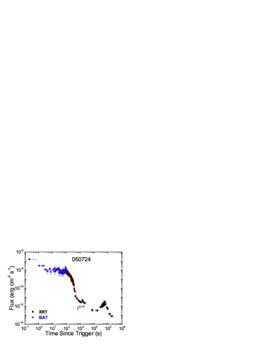
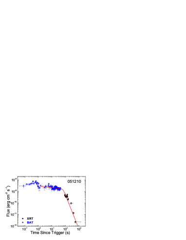
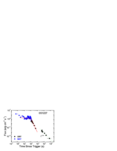
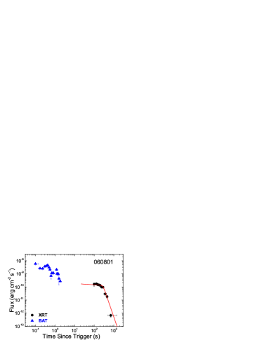
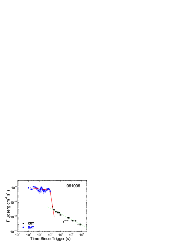
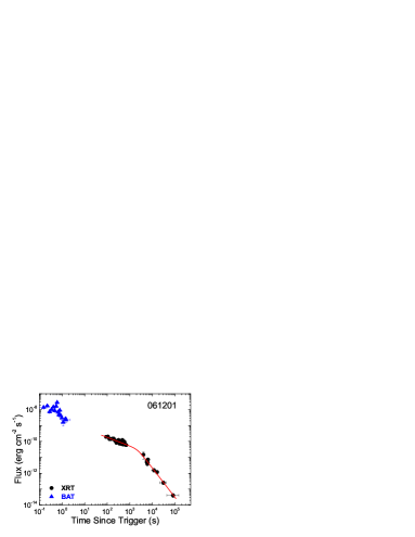
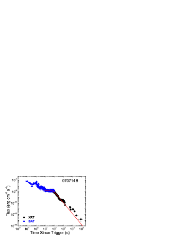
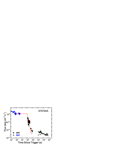
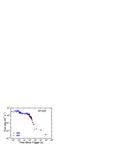
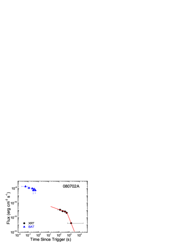
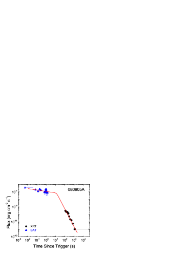
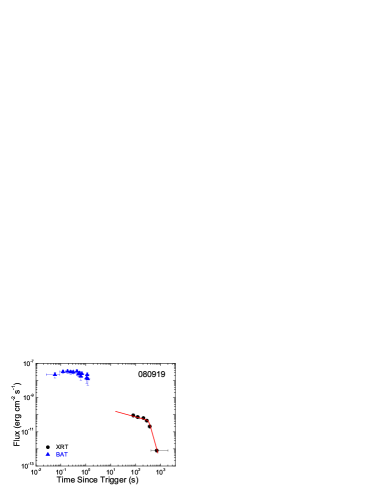
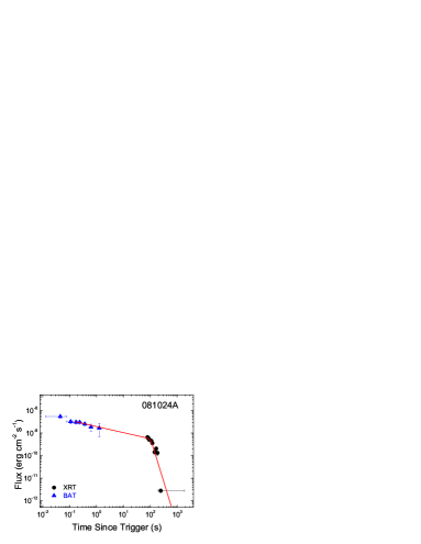
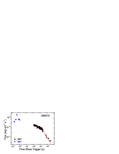
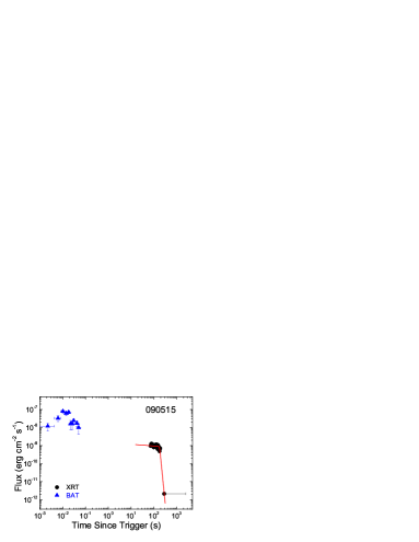
Figure 1.— The BAT-XRT rest-frame light curves of the GRBs in our Internal sample. Blue triangles are BAT data extrapolated to the XRT band, and black points (with error bars) are the XRT data. The red solid curves are the best fits with a smooth power-law model to the data. The green dotted lines are the best fits with power-law model after the steeper decay.

Fig.1— continued.

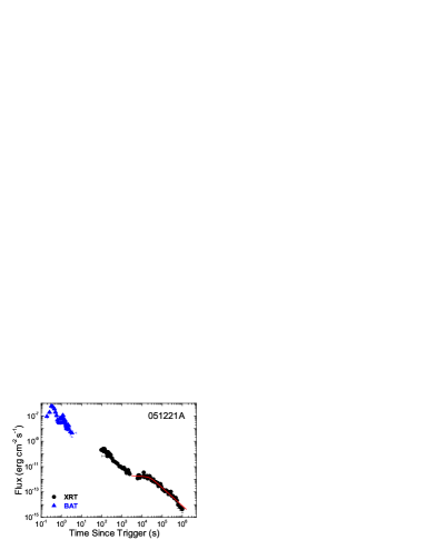
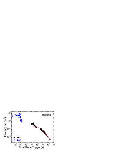
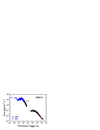
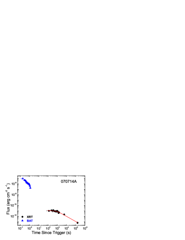
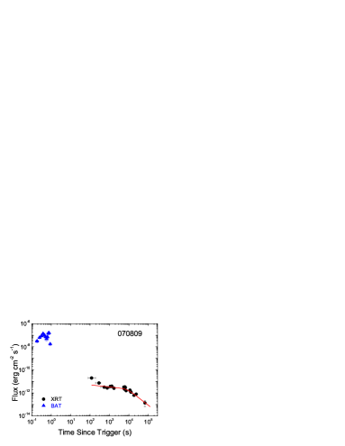
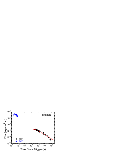
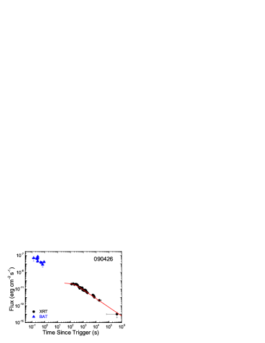
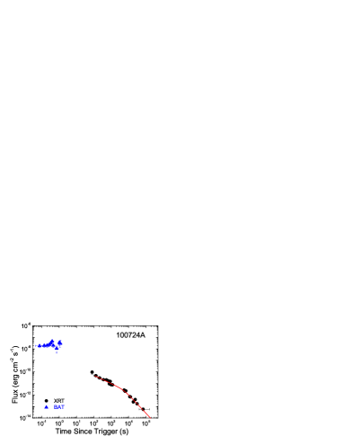
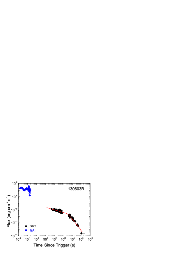
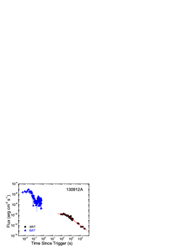
Figure 2.— Similar to Figure 1, but for the External sample.

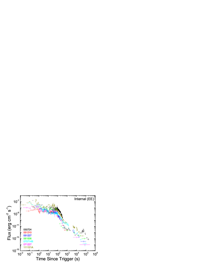
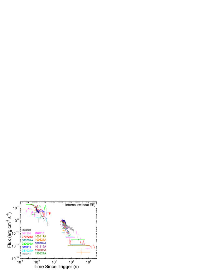
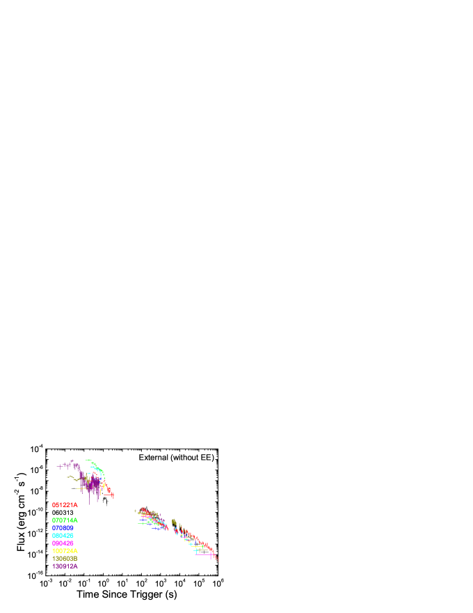
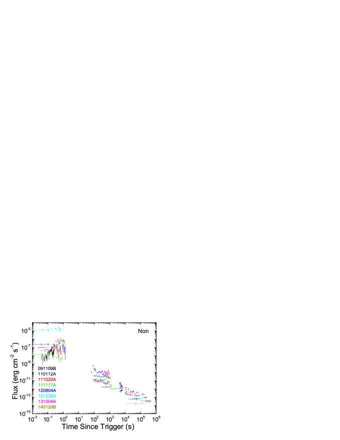
Figure 3.— Ensemble of X-ray light curves (0.3-10 keV) of the GRBs in our Internal sample with EE, Internal sample without EE, External sample, and Non sample.

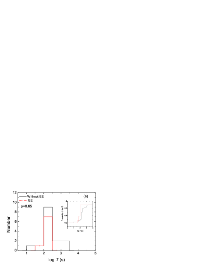
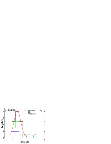
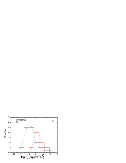
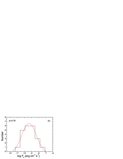
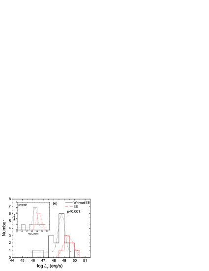
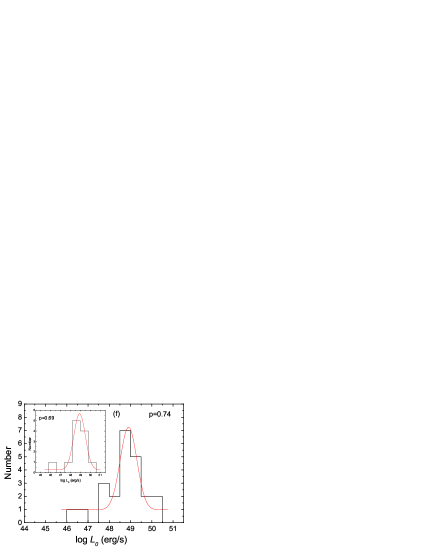
Figure 4.— (a) Duration distributions of the extended emission for EE sample, and the internal plateau emission for the no-EE sample. Inset: the cumulative duration distributions for the EE and no-EE sub-samples. (b) The redshift distribution of all short GRBs with $z$ measurements. The red solid line is the best Gaussian fit with a center value $z_{c}=0.58$. The green and blue histograms are the redshift distributions for the EE and no-EE sub-samples, respectively. (c) The plateau flux distributions of both EE (red, solid line + bar) and no-EE (black, solid line) GRBs in our Internal sample. The dotted lines are the best Gaussian fits to the distributions. (d) A joint fit to the flux distribution of all the GRBs in the Internal plateau (both EE and no-EE included). (e) The plateau luminosity distributions of both EE (red, solid line + bar) and no-EE (black, solid line) GRBs in our Internal sample. The dotted lines are the best Gaussian fits to the distributions. (f) A joint fit to the luminosity distribution of all the GRBs in the Internal plateau (both EE and no-EE included). The insets in (e) and (f) are for the GRBs with measured redshifts only.

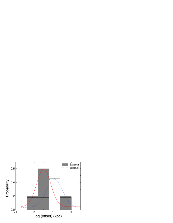
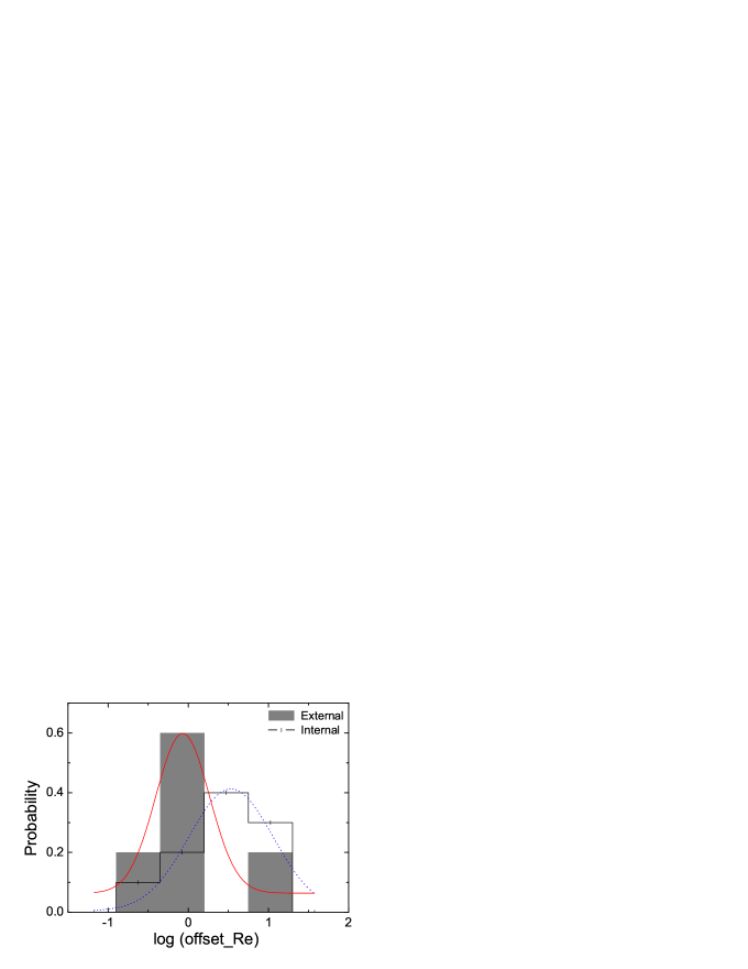
Figure 5.— Distributions of the physical offsets and host-normalized offsets of the Internal and External samples. The solid and dash lines are the best Gaussian fitting for the Internal and External samples, respectively.

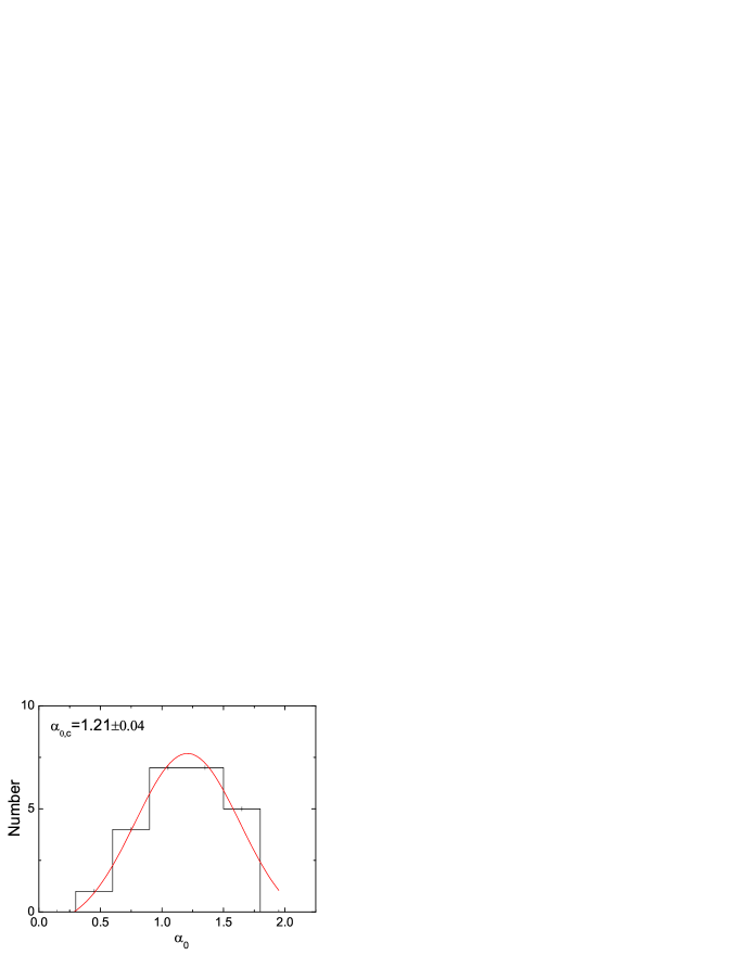
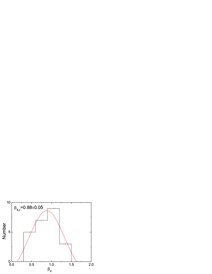
Figure 6.— Distributions of the decay slope $\alpha_{0}$ and spectral index $\beta_{X}$ in the normal decay phase in our External and Non samples. The solid lines are the best Gaussian fits to the distributions.

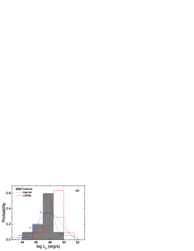
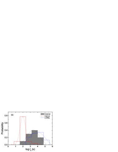
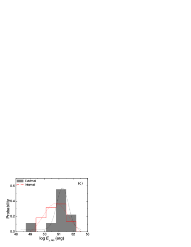
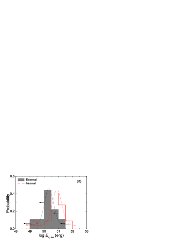
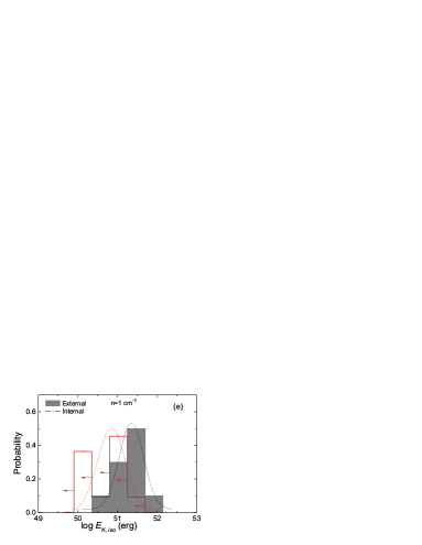
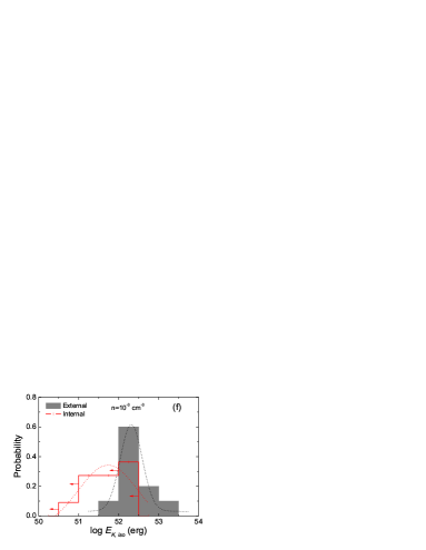
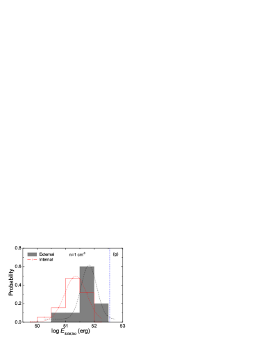
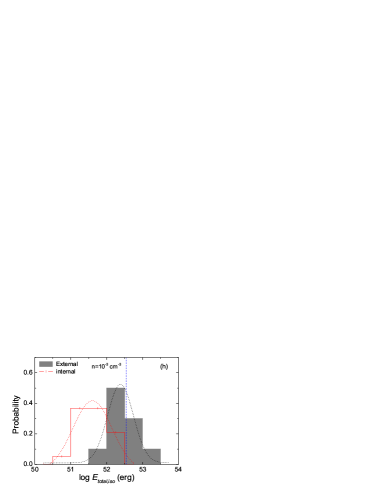
Figure 7.— Comparisons of various properties between the Internal (red, open histogram) sample and the External (black, gray histogram) samples. The best-fit Gaussian profiles are over-plotted with the respective colors. The eight panels denote histograms of $L_{b}$, $t_{b}$, $E_{\rm\gamma,iso}$, $E_{\rm X,iso}$, $E_{\rm K,iso}$ and $E_{\rm total,iso}$, respetively, with the last two parameters plotted twice for two different medium densities, $n=1,10^{-3}~{}{\rm cm^{-3}}$. The vertical dotted line in panels (g) and (h) denotes the total rotation energy budget of a millisecond magnetar. If no redshift is measured, then $z=0.58$ is adopted in the calculations.

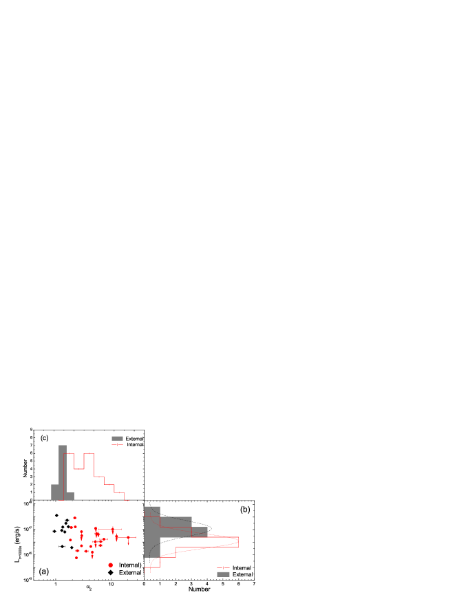
Figure 8.— One-dimensional (panels (b) and (c)) and two-dimensional (panel (a)) $L(t=1000~{}{\rm s})-\alpha_{2}$ distributions of the GRBs in our samples. The red diamonds and black dots denote the Internal and External samples, respectively, and the arrows indicate the upper limits.

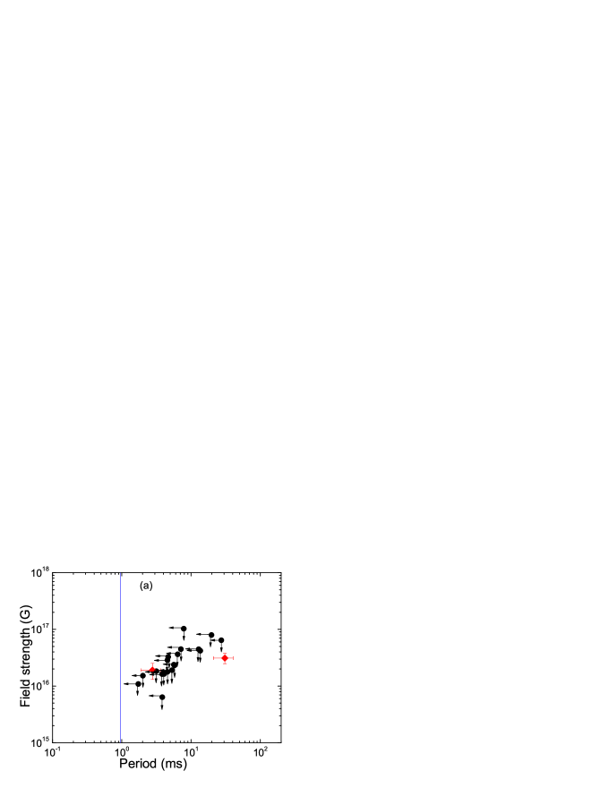
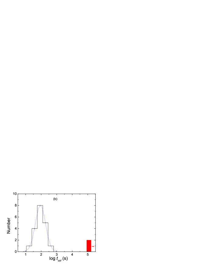
Figure 9.— (a) Inferred magnetar parameters, initial spin period $P_{0}$ vs. surface polar cap magnetic field strength $B_{p}$ derived for our Internal sample. The red diamonds indicate GRB 061201 and GRB 070714B, which have $\tau$ measured from $t_{b}$. All the other GRBs only have the lower limit of $\tau$. The arrows denote upper limits. The vertical solid line is the break-up spin period limit for a neutron star (Lattimer & Prakash 2004). (b) The distribution of the collapse time for our Internal sample. The dotted line is the best Gaussian profile fit.

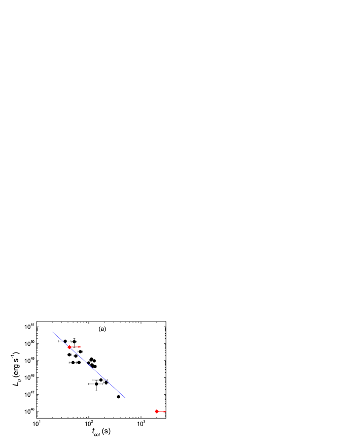
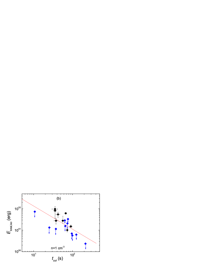
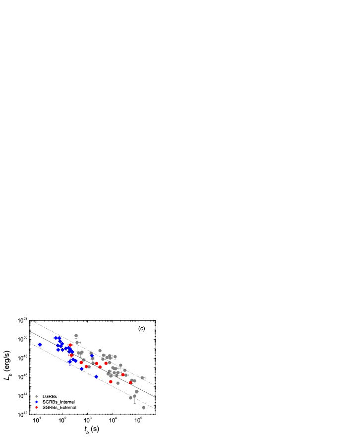
Figure 10.— (a) $L_{0}-t_{col}$ anti-correlation for our Internal samples. The red diamonds are GRB 061201 and GRB 070714B, and the arrows denote the lower limits of the collapse time. (b) The $E_{\rm total,iso}-t_{col}$ anti-correlation for our Internal sample using $n=1~{}{\rm cm^{-3}}$ to calculate $E_{\rm K,iso}$. The blue diamonds indicate the upper limits to calculate $E_{\rm K,iso}$, and the red solid line is the best-fitting line. (c) The empirical $L_{b}-t_{b}$ correlation derived from the short GRBs in our sample (red for External and blue for Internal samples) compared with the Dainotti relation for long GRBs (gray). The solid line is the best power-law fit to the SGRBs sample, and the two dotted lines denote the 2$\sigma$ region of the fit.

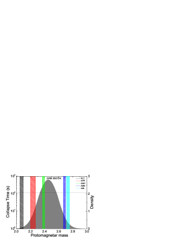
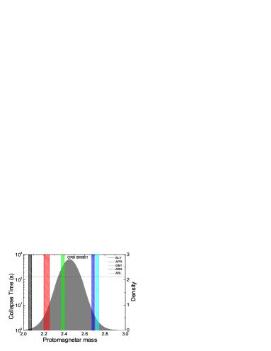
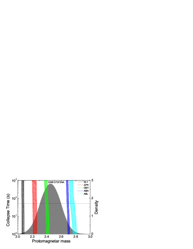
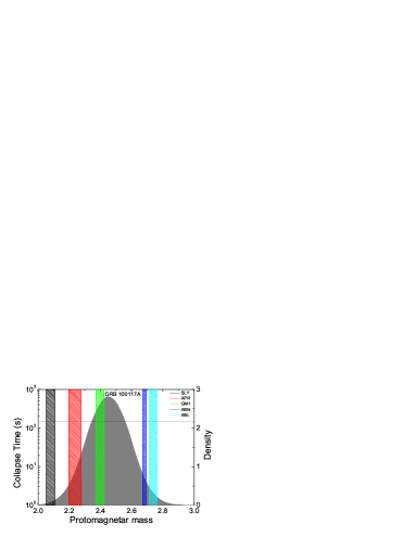
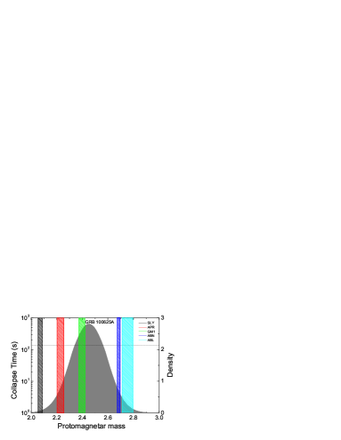
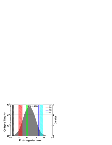
Figure 11.— Collapse time as a function of the protomagnetar mass. The shaded region is the protomagnetar mass distribution derived from the total mass distribution of the Galactic NS$-$NS binary systems. The predicted results for 5 equations of state are shown in each panel: SLy (black), APR (red), GM1 (green), AB-N (blue), and AB-L (cyan). The horizontal dotted line is the observed collapse time for each GRB.

References

- Akmal et al. (1998) Akmal, A., Pandharipande, V. R., & Ravenhall, D. G. 1998, PhRevC, 58, 1804
- Arnett & Bowers (1977) Arnett, W. D., & Bowers, R. L. 1977, ApJS, 33, 415
- Bannister et al. (2012) Bannister, K. W., Murphy, T., Gaensler, B. M., & Reynolds, J. E. 2012, ApJ, 757, 38
- Barthelmy et al. (2013) Barthelmy, S. D., Baumgartner, W. H., Cummings, J. R., et al. 2013, GCN, 14741, 1
- Barthelmy et al. (2005) Barthelmy, S. D., Chincarini, G., Burrows, D. N., et al. 2005, Natur, 438, 994
- Berger et al. (2005) Berger, E., Price, P. A., Cenko, S. B., et al. 2005, Natur, 438, 988
- Berger (2014) Berger, E. 2014, ARA&A, 52, 43
- Bloom et al. (2002) Bloom, J. S., Kulkarni, S. R., & Djorgovski, S. G. 2002, AJ, 123, 1111
- Bloom et al. (1999) Bloom, J. S., Kulkarni, S. R., Djorgovski, S. G., et al. 1999, Natur, 401, 453
- Bloom et al. (2006) Bloom, J. S., Prochaska, J. X., Pooley, D., et al. 2006, ApJ, 638, 354
- Bucciantini et al. (2012) Bucciantini, N., Metzger, B. D., Thompson, T. A., & Quataert, E. 2012, MNRAS, 419, 1537
- Butler et al. (2007) Butler, N. R., Kocevski, D., Bloom, J. S., & Curtis, J. L. 2007, ApJ, 671, 656
- Campana et al. (2006) Campana, S., Mangano, V., Blustin, A. J., et al. 2006, Natur, 442, 1008
- Campana et al. (2006) Campana, S., Tagliaferri, G., Lazzati, D., et al. 2006, A&A, 454, 113
- Ciolfi & Siegel (2015) Ciolfi, R., & Siegel, D. M. 2015, ApJL, 798, L36
- Cook et al. (1994) Cook, G. B., Shapiro, S. L., & Teukolsky, S. A. 1994, ApJ, 424, 823
- Cucchiara et al. (2013) Cucchiara, A., Prochaska, J. X., Perley, D., et al. 2013, ApJ, 777, 94
- Dai & Lu (1998) Dai, Z. G., & Lu, T. 1998, A&A, 333, L87
- Dai et al. (2006) Dai, Z. G., Wang, X. Y., Wu, X. F., & Zhang, B. 2006, Sci, 311, 1127
- Dainotti et al. (2008) Dainotti, M. G., Cardone, V. F., & Capozziello, S. 2008, MNRAS, 391, L79
- Dainotti et al. (2015) Dainotti, M. G., Del Vecchio, R., Shigehiro, N., & Capozziello, S. 2015, ApJ, 800, 31
- Dainotti et al. (2013) Dainotti, M. G., Petrosian, V., Singal, J., & Ostrowski, M. 2013, ApJ, 774, 157
- Dainotti et al. (2010) Dainotti, M. G., Willingale, R., Capozziello, S., Fabrizio Cardone, V., & Ostrowski, M. 2010, ApJL, 722, L215
- Della Valle et al. (2006) Della Valle, M., Chincarini, G., Panagia, N., et al. 2006, Natur, 444, 1050
- Deng & Zhang (2014) Deng, W., & Zhang, B. 2014, ApJL, 783, LL35
- Douchin & Haensel (2001) Douchin, F., & Haensel, P. 2001, A&A, 380, 151
- Duez et al. (2006) Duez, M. D., Liu, Y. T., Shapiro, S. L., Shibata, M., & Stephens, B. C. 2006, PhRvL, 96, 031101
- Eichler et al. (1989) Eichler, D., Livio, M., Piran, T., & Schramm, D. N. 1989, Natur, 340, 126
- Evans et al. (2009) Evans, P. A., Beardmore, A. P., Page, K. L., et al. 2009, MNRAS, 397, 1177
- Falcke & Rezzolla (2014) Falcke, H., & Rezzolla, L. 2014, A&A, 562, AA137
- Fan et al. (2005) Fan, Y. Z., Zhang, B., Kobayashi, S., & Mészáros, P. 2005, ApJ, 628, 867
- Fan et al. (2013a) Fan, Y.-Z., Wu, X.-F., & Wei, D.-M. 2013a, PhRvD, 88, 067304
- Fan et al. (2013b) Fan, Y.-Z., Yu, Y.-W., Xu, D., et al. 2013b, ApJL, 779, LL25
- Fong & Berger (2013) Fong, W., & Berger, E. 2013, ApJ, 776, 18
- Fong et al. (2013) Fong, W., Berger, E., Chornock, R., et al. 2013, ApJ, 769, 56
- Fong et al. (2011) Fong, W., Berger, E., Chornock, R., et al. 2011, ApJ, 730, 26
- Fong et al. (2010) Fong, W., Berger, E., & Fox, D. B. 2010, ApJ, 708, 9
- Fox et al. (2005) Fox, D. B., Frail, D. A., Price, P. A., et al. 2005, Natur, 437, 845
- Fruchter et al. (2006) Fruchter, A. S., Levan, A. J., Strolger, L., et al. 2006, Natur, 441, 463
- Fynbo et al. (2006) Fynbo, J. P. U., Watson, D., Thöne, C. C., et al. 2006, Natur, 444, 1047
- Gal-Yam et al. (2006) Gal-Yam, A., Fox, D. B., Price, P. A., et al. 2006, Natur, 444, 1053
- Galama et al. (1998) Galama, T. J., Vreeswijk, P. M., van Paradijs, J., et al. 1998, Natur, 395, 670
- Gao et al. (2013) Gao, H., Lei W.-H., Zou Y.-C., Wu X.-F., Zhang B., 2013a, NewAR, 57, 141
- Gao et al. (2013) Gao, H., Ding, X., Wu, X.-F., Zhang, B., & Dai, Z.-G. 2013b, ApJ, 771, 86
- Gao et al. (2014) Gao, H., Li, Z., & Zhang, B. 2014, ApJ, 788, 189
- Gao & Fan (2006) Gao, W.-H., & Fan, Y.-Z. 2006, ChJAA, 6, 513
- Gehrels et al. (2006) Gehrels, N., Norris, J. P., Barthelmy, S. D., et al. 2006, Natur, 444, 1044
- Gehrels et al. (2005) Gehrels, N., Sarazin, C. L., O’Brien, P. T., et al. 2005, Natur, 437, 851
- Giacomazzo & Perna (2013) Giacomazzo, B., & Perna, R. 2013, ApJL, 771, LL26
- Glendenning & Moszkowski (1991) Glendenning, N. K., & Moszkowski, S. A. 1991, PhRvL, 67, 2414
- Gompertz et al. (2014) Gompertz, B. P., O’Brien, P. T., & Wynn, G. A. 2014, MNRAS, 438, 240
- Gompertz et al. (2013) Gompertz, B. P., O’Brien, P. T., Wynn, G. A., & Rowlinson, A. 2013, MNRAS, 431, 1745
- Hjorth et al. (2003) Hjorth, J., Sollerman, J., Møller, P., et al. 2003, Natur, 423, 847
- Hotokezaka et al. (2013) Hotokezaka, K., Kiuchi, K., Kyutoku, K. et al. 2013, PhRvD, 87, 024001
- Hullinger et al. (2005) Hullinger, D., Barbier, L., Barthelmy, S., et al. 2005, GCN, 4400, 1
- Kann et al. (2011) Kann, D. A., Klose, S., Zhang, B., et al. 2011, ApJ, 734, 96
- Kiziltan et al. (2013) Kiziltan, B., Kottas, A., De Yoreo, M., & Thorsett, S. E. 2013, ApJ, 778, 66
- Kouveliotou et al. (1993) Kouveliotou, C., Meegan, C. A., Fishman, G. J., et al. 1993, ApJL, 413, L101
- Krimm et al. (2013) Krimm, H. A., Barthelmy, S. D., Baumgartner, W. H., et al. 2013, GRB Coordinates Network, 15216, 1
- Lasky et al. (2014) Lasky, P. D., Haskell, B., Ravi, V., Howell, E. J., & Coward, D. M. 2014, PhRevD, 89, 047302
- Lei et al. (2013) Lei, W.-H., Zhang, B., & Liang, E.-W. 2013, ApJ, 765, 125
- Leibler & Berger (2010) Leibler, C. N., & Berger, E. 2010, ApJ, 725, 1202
- Liang et al. (2007) Liang, E.-W., Zhang, B.-B., & Zhang, B. 2007, ApJ, 670, 565
- Liu et al. (2012) Liu, T., Liang, E.-W., Gu, W.-M., et al. 2012, ApJ, 760, 63
- Lorimer et al. (2007) Lorimer, D. R., Bailes, M., McLaughlin, M. A., Narkevic, D. J., & Crawford, F. 2007, Science, 318, 777
- Lü & Zhang (2014) Lü, H.-J., & Zhang, B. 2014, ApJ, 785, 74
- Lü et al. (2014) Lü, H.-J., Zhang, B., Liang, E.-W., Zhang, B.-B., & Sakamoto, T. 2014, MNRAS, 442, 1922
- Lyford et al. (2003) Lyford, N. D., Baumgarte, T. W., & Shapiro, S. L. 2003, ApJ, 583, 410
- Lyons et al. (2010) Lyons, N., O’Brien, P. T., Zhang, B., et al. 2010, MNRAS, 402, 705
- MacFadyen & Woosley (1999) MacFadyen, A. I., & Woosley, S. E. 1999, ApJ, 524, 262
- Markwardt (2009) Markwardt, C. B. 2009, adass, 411, 251
- Markwardt et al. (2010) Markwardt, C. B., Barthelmy, S. D., Baumgartner, W. H., et al. 2010, GCN, 10972, 1
- Metzger et al. (2011) Metzger, B. D., Giannios, D., Thompson, T. A., Bucciantini, N., & Quataert, E. 2011, MNRAS, 413, 2031
- Metzger et al. (2008) Metzger, B. D., Quataert, E., & Thompson, T. A. 2008, MNRAS, 385, 1455
- Metzger & Piro (2014) Metzger, B. D., & Piro, A. L. 2014, MNRAS, 439, 3916
- Norris & Bonnell (2006) Norris, J. P., & Bonnell, J. T. 2006, ApJ, 643, 266
- O’Brien et al. (2006) O’Brien, P. T., Willingale, R., Osborne, J., et al. 2006, ApJ, 647, 1213
- Paczynski (1986) Paczynski, B. 1986, ApJL, 308, L43
- Paczynski (1991) Paczynski B., 1991, AcA, 41, 257
- Panaitescu & Kumar (2002) Panaitescu, A., & Kumar, P. 2002, ApJ, 571, 779
- Perley et al. (2009) Perley, D. A., Metzger, B. D., Granot, J., et al. 2009, ApJ, 696, 1871
- Popham et al. (1999) Popham, R., Woosley, S. E., & Fryer, C. 1999, ApJ, 518, 356
- Ravi & Lasky (2014) Ravi, V., & Lasky, P. D. 2014, MNRAS, 441, 2433
- Rezzolla et al. (2011) Rezzolla, L., Giacomazzo, B., Baiotti, L., et al. 2011, ApJL, 732, LL6
- Rezzolla & Kumar (2015) Rezzolla, L., & Kumar, P. 2015, ApJ, 802, 95
- Rosswog et al. (2003) Rosswog, S., Ramirez-Ruiz, E., & Davies, M. B. 2003, MNRAS, 345, 1077
- Rowlinson et al. (2014) Rowlinson, A., Gompertz, B. P., Dainotti, M., et al. 2014, MNRAS, 443, 1779
- Rowlinson et al. (2013) Rowlinson, A., O’Brien, P. T., Metzger, B. D., Tanvir, N. R., & Levan, A. J. 2013, MNRAS, 430, 1061
- Rowlinson et al. (2010) Rowlinson, A., O’Brien, P. T., Tanvir, N. R., et al. 2010, MNRAS, 409, 531
- Sakamoto et al. (2008) Sakamoto, T., Barthelmy, S. D., Barbier, L., et al. 2008, ApJS, 175, 179
- Sakamoto et al. (2011) Sakamoto, T., Barthelmy, S. D., Baumgartner, W. H., et al. 2011, ApJS, 195, 2
- Shapiro & Teukolsky (1983) Shapiro, S., & Teukolsky, S. 1983, The Physics of Compact Objects
- Siegel et al. (2014) Siegel, D. M., Ciolfi, R., & Rezzolla, L. 2014, ApJL, 785, LL6
- Stanek et al. (2003) Stanek, K. Z., Matheson, T., Garnavich, P. M., et al. 2003, ApJL, 591, L17
- Thoene et al. (2010) Thoene, C. C., de Ugarte Postigo, A., Vreeswijk, P., et al. 2010, GCN, 10971, 1
- Thompson (1994) Thompson, C. 1994, MNRAS, 270, 480
- Thornton et al. (2013) Thornton, D., Stappers, B., Bailes, M., et al. 2013, Science, 341, 53
- Troja et al. (2007) Troja, E., Cusumano, G., O’Brien, P. T., et al. 2007, ApJ, 665, 599
- Usov (1992) Usov, V. V. 1992, Natur, 357, 472
- Valentim et al. (2011) Valentim, R., Rangel, E., & Horvath, J. E. 2011, MNRAS, 414, 1427
- Wheeler et al. (2000) Wheeler, J. C., Yi, I., Höflich, P., & Wang, L. 2000, ApJ, 537, 810
- Willingale et al. (2007) Willingale, R., O’Brien, P. T., Osborne, J. P., et al. 2007, ApJ, 662, 1093
- Willingale et al. (2010) Willingale, R., Genet, F., Granot, J., & O’Brien, P. T. 2010, MNRAS, 403, 1296
- Woosley (1993) Woosley, S. E. 1993, ApJ, 405, 273
- Xu et al. (2013) Xu, D., de Ugarte Postigo, A., Leloudas, G., et al. 2013, ApJ, 776, 98
- Yost et al. (2003) Yost, S. A., Harrison, F. A., Sari, R., & Frail, D. A. 2003, ApJ, 597, 459
- Yu et al. (2010) Yu, Y.-W., Cheng, K. S., & Cao, X.-F. 2010, ApJ, 715, 477
- Yu et al. (2013) Yu, Y.-W., Zhang, B., & Gao, H. 2013, ApJL, 776, LL40
- Zhang (2014) Zhang, B. 2014, ApJL, 780, LL21
- Zhang (2013) Zhang, B. 2013, ApJL, 763, LL22
- Zhang et al. (2007) Zhang, B., Liang, E., Page, K. L., et al. 2007a, ApJ, 655, 989
- Zhang & Mészáros (2004) Zhang, B., & Mészáros, P. 2004, International Journal of Modern Physics A, 19, 2385
- Zhang & Mészáros (2001) Zhang, B., & Mészáros, P. 2001, ApJL, 552, L35
- Zhang et al. (2007) Zhang, B., Zhang, B.-B., Liang, E.-W., et al. 2007b, ApJL, 655, L25
- Zhang et al. (2009) Zhang, B., Zhang, B.-B., Virgili, F. J., et al. 2009, ApJ, 703, 1696
- Zhang et al. (2007) Zhang, B.-B., Liang, E.-W., & Zhang, B. 2007c, ApJ, 666, 1002
- Zheng et al. (2014) Zheng, Z., Ofek, E. O., Kulkarni, S. R., Neill, J. D., & Juric, M. 2014, ApJ, 797, 71
- Zhou et al. (2014) Zhou, B., Li, X., Wang, T., Fan, Y.-Z., & Wei, D.-M. 2014, PhRevD, 89, 107303