Gamma-ray burst early optical afterglows: implications for the initial Lorentz factor and the central engine

Abstract

Early optical afterglows have been observed from GRB 990123, GRB 021004, and GRB 021211, which reveal rich emission features attributed to reverse shocks. It is expected that Swift will discover many more early afterglows. Here we investigate in a unified manner both the forward and the reverse external shock emission components, and introduce a straightforward recipe for directly constraining the initial Lorentz factor of the fireball using early optical afterglow data. The scheme is largely independent of the shock microphysics. We identify two types of combinations of the reverse and forward shock emission, and explore their parameter regimes. We also discuss a possible diagnostic for magnetized ejecta. There is evidence that the central engine of GRB 990123 is strongly magnetized.

1. Introduction

The standard Gamma-ray burst (GRB) afterglow model (Mészáros & Rees 1997a; Sari, Piran & Narayan 1998) invokes synchrotron emission of electrons from the forward external shock, and has been proven successful in interpreting the late time broadband afterglows. At these late times the fireball is already decelerated and has entered a self-similar regime, in which precious information about the early ultra-relativistic phase is lost. In the very early afterglow epoch, the emission from the reverse shock propagating into the fireball itself also plays a noticeable role, especially in the low frequency bands, e.g. optical or radio (Mészáros & Rees 1997a; Sari & Piran 1999b), and information about the fireball initial Lorentz factor could be in principle retrieved from the reverse shock data. For a long time, evidence for reverse shock emission was available only from GRB 990123 (Akerlof et al. 1999; Sari & Piran 1999a; Mészáros & Rees 1999; Kobayashi & Sari 2000). Recently, thanks to prompt localizations of GRBs by the High Energy Transient Explorer 2 (HETE-2) (e.g. Shirasaki et al. 2002; Crew et al. 2002) and rapid follow-ups by robotic optical telescopes (e.g. Fox 2002; Li et al. 2002; Fox & Price 2002; Park et al. 2002; Wolzniak et al. 2002), reverse shock emission has also been identified from GRB 021211 (Fox et al. 2003; Li et al. 2003; Wei 2003) and possibly also from GRB 021004 (Kobayashi & Zhang 2003a). It is expected that the Swift mission will record many GRB early optical afterglows after its launch scheduled in December 2003, which will unveil a rich phenomenology of early afterglows.

Here we propose a paradigm to analyze the early optical afterglow data, starting from tens of seconds after the gamma-ray trigger. By combining the emission information from both the forward and the reverse shocks, we discuss a way to derive or constrain the initial Lorentz factor of the fireball directly from the observables. The method does not depend on the absolute values of the poorly-known shock microphysics (e.g. the electron and magnetic equipartition parameters $\epsilon_{e}$ and $\epsilon_{B}$, and the electron power-law index $p$). We also categorize the early optical afterglows into two types and discuss the parameter regimes for both cases.

2. Forward and reverse shock comparison

We consider a relativistic shell (fireball ejecta) with an isotropic equivalent energy $E$ and an initial Lorentz factor $\gamma_{0}$ expanding into a homogeneous interstellar medium (ISM) with particle number density $n$ at a redshift $z$. Some GRB afterglows may occur in the progenitors’ stellar winds (e.g. Chevalier & Li 1999). The combined reverse vs. forward shock emission for the wind environment is easy to be distinguished from what is discussed here, and has been discussed separately (Kobayashi & Zhang 2003b).

For the homogeneous ISM case, in the observer’s frame, one can define a timescale when the accumulated ISM mass is $1/\gamma_{0}$ of the ejecta mass, i.e., $t_{\gamma}=[(3E/4\pi\gamma_{0}^{2}nm_{p}c^{2})^{1/3}/2\gamma_{0}^{2}c](1+z)$. This is the fireball deceleration time if the burst duration $T<t_{\gamma}$ (the so-called thin-shell regime, Sari & Piran 1995). For $T>t_{\gamma}$, the deceleration time is delayed to $T$ (thick-shell regime). The critical condition $T=t_{\gamma}$ defines a critical initial Lorentz factor

$$\gamma_{c}\simeq 125E_{52}^{1/8}n^{-1/8}T_{2}^{-3/8}\left(\frac{1+z}{2}\right)^{3/8}~{},$$ (1)

where the convention $Q=10^{x}Q_{x}$ is used. So one has $\gamma_{0}<\gamma_{c}$ for the thin-shell case, and $\gamma_{0}>\gamma_{c}$ for the thick-shell case. When the reverse shock crosses the shell, the observer time and the ejecta Lorentz factor are (Sari & Piran 1995; Kobayashi, Piran & Sari 1999)

$$t_{\times}={\rm max}(t_{\gamma},T), \gamma_{\times}={\rm min}(\gamma_{0},\gamma_{c}),$$ (2)

where the first and second values in the above expressions correspond to the thin and thick shell cases, respectively. Since $T$ and $z$ can be directly measured, e.g. by Swift, and $E$ and $n$ could be inferred from broadband afterglow fitting (e.g. Panaitescu & Kumar 2001), $\gamma_{c}$ is essentially an observable in an idealized observational campaign. Some estimates (or fits) about the microphysics parameters ($\epsilon_{e}$, $\epsilon_{B}$, $p$, etc.) have to be involved when inferring $E$ and $n$, but $\gamma_{c}$ is insensitive to the inaccuracy of measuring $n$ and $E$. The correction to $\gamma_{c}$ is less than a factor of 2 even if the uncertainty of either $E$ or $n$ is by a factor of 100.

The forward shock synchrotron spectrum can be approximated as a four-segment power-law with breaks at the cooling frequency $\nu_{c}$, typical frequency $\nu_{m}$ and the self-absorption frequency $\nu_{a}$ (Sari et al. 1998). So is the reverse shock emission spectrum at $t<t_{\times}$. For $t>t_{\times}$, there is essentially no emission above $\nu_{c}$ for the reverse shock emission. For both shocks, the typical frequency, cooling frequency and the peak flux scale as $\nu_{m}\propto\gamma B\gamma_{e}^{2}$, $\nu_{c}\propto\gamma^{-1}B^{-3}t^{-2}$, and $F_{\nu,m}\propto\gamma BN_{e}$, where $\gamma$ is the bulk Lorentz boost, $B$ is the comoving magnetic field, $\gamma_{e}$ is the typical electron Lorentz factor in the shock-heated region, and $N_{e}$ is the total number of emitting electrons. Using similar analyses in Kobayashi & Zhang 2003a, we can derive

$$\frac{\nu_{m,r}(t_{\times})}{\nu_{m,f}(t_{\times})} \sim \hat{\gamma}^{-2}{\cal R}_{B}~{},$$ (3)

$$\frac{\nu_{c,r}(t_{\times})}{\nu_{c,f}(t_{\times})} \sim {{\cal R}_{B}}^{-3}~{},$$ (4)

$$\frac{F_{\nu,m,r}(t_{\times})}{F_{\nu,m,f}(t_{\times})} \sim \hat{\gamma}{\cal R}_{B}~{},$$ (5)

where

$$\hat{\gamma}\equiv\frac{\gamma_{\times}^{2}}{\gamma_{0}}={\rm min}(\gamma_{0},\frac{\gamma_{c}^{2}}{\gamma_{0}})\leq\gamma_{c}~{},$$ (6)

$${\cal R}_{B}\equiv\frac{B_{r}}{B_{f}}=\left(\frac{\epsilon_{B,r}}{\epsilon_{B,f}}\right)^{1/2}~{},$$ (7)

and the subcripts ‘f’ and ‘r’ indicate forward and reverse shock, respectively. By deriving the second equation in eq.(7), we have taken into account the fact that the internal energy densities are the same in both the forward- and reverse-shocked regions, as evident in the standard hydrodynamical shock jump conditions. We have also assumed that the $\epsilon_{e}$ and $p$ parameters are the same for both the forward and reverse-shocked regions, but with different $\epsilon_{B}$’s (as parameterized by ${\cal R}_{B}$). The reason we introduce the ${\cal R}_{B}$ parameter is that in some central engine models (e.g. Usov 1992; Mészáros & Rees 1997b; Wheeler et al. 2000), the fireball wind may be endowed with “primordial” magnetic fields, so that in principle $B_{r}$ could be higher than $B_{f}$. We note that all the previous investigations have assumed the same microphysics parameters in both shocks.

The forward shock emission is likely to be in the “fast cooling” regime ($\nu_{c,f}<\nu_{m,f}$) initially and in the “slow cooling” regime ($\nu_{c,f}>\nu_{m,f}$) at later times (Sari et al. 1998). For the reverse shock emission, it can be deduced from eqs. (3, 4) and eq.(11) of Sari et al. (1998) that slow cooling ($\nu_{c,r}>\nu_{m,r}$) is generally valid as long as ${\cal R}_{B}$ is not much greater than unity.

The lightcurves can be derived by specifying the temporal evolution of $\nu_{m}$, $\nu_{c}$, and $F_{\nu,m}$. To first order, in the forward shock (Mészáros & Rees 1997a) we have

$$\nu_{m,f}\propto t^{-3/2}, F_{\nu,m,f}\propto t^{0}$$ (8)

while in the reverse shock for $t>t_{\times}$ (Kobayashi 2000) we have approximately

$$\nu_{m,r}\propto t^{-3/2}, F_{\nu,m,r}\propto t^{-1}$$ (9)

The optical-band lightcurve for the forward shock is well-described by the “low-frequency” case of Sari et al. (1998, their Fig.2b), characterized by a turnover of the temporal indices from 1/2 to $\sim-1$ at the peak time $t_{p,f}$ (at which $\nu_{m,f}$ crosses the observational band, e.g. the typical R-band frequency $\nu_{R}$). The optical lightcurve for the reverse shock emission is more complicated, depending on whether the shell is thin or thick, whether it is in the slow or fast cooling regime, and how $\nu_{R}$ compares with $\nu_{m,r}(t_{\times})$ and $\nu_{c,r}(t_{\times})$ (see Kobayashi 2000 for a complete discussion). For reasonable parameters, however, the cases of $\nu_{R}>\nu_{c,r}$ and $\nu_{R}<\nu_{a,r}$ are unlikely, and even if these conditions are satisfied, they do not produce interesting reverse shock signatures. Defining

$${\cal R}_{\nu}\equiv\frac{\nu_{R}}{\nu_{m,r}(t_{\times})},$$ (10)

and specifying the slow-cooling case (which is reasonable for a large sector of parameter regimes, see Kobayashi 2000), the reverse shock lightcurves are then categorized into four cases with various temporal indices separated by various break times. The four cases with their typical temporal power-law indices (in parentheses), which correspond to the thick and thin solid lines in Fig.2a and Fig.3a of Kobayashi (2000), are: (i) thin shell ${\cal R}_{\nu}>1$: $\sim(5,-2)$; (ii) thin shell ${\cal R}_{\nu}<1$: $\sim(5,-1/2,-2)$: (iii) thick shell ${\cal R}_{\nu}>1$: $\sim(1/2,-2)$; (iv) thick shell ${\cal R}_{\nu}<1$: $\sim(1/2,-1/2,-2)$. We note that in all four cases, the final temporal power-law index is $\sim-2$, corresponding to adiabatic cooling of the already accelerated electrons at $t_{\times}$, with $\nu_{R}>\nu_{m,r}$. Strictly speaking, by writing the final lightcurve as $F_{\nu,r}=F_{\nu,m,r}(\nu/\nu_{m,r})^{-(p-1)/2}\propto t^{-\alpha}$, and making use of eq.(9), we have

$$\alpha=\frac{3p+1}{4},$$ (11)

where $p$ is the power law index of the electrons in the reverse shock region. We can see that $\alpha\sim 2$ for typical $p$ values. Going backwards in time, this well-known $F_{\nu,r}\propto t^{-2}$ reverse shock lightcurve ends at $t_{\times}$ for ${\cal R}_{\nu}>1$ (with a rising lightcurve before that), but at the time when $\nu_{m,r}$ crosses $\nu_{R}$ for ${\cal R}_{\nu}<1$ (with a flatter declining lightcurve, $F_{\nu,r}\propto t^{-1/2}$, before) (Fig.1).

We define as $t_{p,r}$ the time when the $F_{\nu,r}\propto t^{-2}$ lightcurve starts and define the corresponding reverse shock spectral flux as $F_{\nu,p,r}$ (Fig.1). The lightcurve point $(t_{p,r},F_{\nu,p,r})$ is generally called the reverse shock peak, but strictly this is valid only when ${\cal R}_{\nu}>1$ (in which case $t_{p,r}=t_{\times}$). On the other hand, it is natural to define the forward shock peak at $(t_{p,f},F_{\nu,p,f})$ (Fig.1), where $F_{\nu,p,f}=F_{\nu,m,f}=$constant (eq.[8]). For practical purposes, it is illustrative to derive the ratio of the two peak times and that of the two peak fluxes by making use of eqs. (3), (5), (8), (9) and (11), i.e.

$${{\cal R}_{t}}\equiv\frac{t_{p,f}}{t_{p,r}}=\left\{\begin{array}[]{@{\,}ll}\hat{\gamma}^{4/3}{{\cal R}_{B}}^{-2/3}{\cal R}_{\nu}^{-2/3},&{\cal R}_{\nu}>1,\\ \hat{\gamma}^{4/3}{{\cal R}_{B}}^{-2/3},&{\cal R}_{\nu}<1,\end{array}\right.$$ (12)

$${{\cal R}_{F}}\equiv\frac{F_{\nu,p,r}}{F_{\nu,p,f}}=\left\{\begin{array}[]{@{\,}ll}\hat{\gamma}{\cal R}_{B}{\cal R}_{\nu}^{-2(\alpha-1)/3},&{\cal R}_{\nu}>1,\\ \hat{\gamma}{\cal R}_{B}{\cal R}_{\nu}^{2/3},&{\cal R}_{\nu}<1.\end{array}\right.$$ (13)

Notice that we have intentionally defined both ${{\cal R}_{t}}$ and ${{\cal R}_{F}}$ to be (usually) larger than unity, and that these expressions are valid regardless of whether the shell is thin or thick. Since we are working on the “ratios” of the quantities for both shocks, the absolute values of the microphysics parameters do not enter the problem. Instead, our expressions involve relative ratios of these parameters, so that they cancel out in eqs.(12) and (13) if they are the same in both shocks, as we have assumed in this paper (except for ${\cal R}_{B}$).

3. A recipe to constrain the initial Lorentz factor

Reverse shock emission data have been used to estimate the initial Lorentz factor of GRB 990123 (Sari & Piran 1999a; Kobayashi & Sari 2000; Wang, Dai & Lu 2000; Soderberg & Ramirez-Ruiz 2002; Fan et al. 2002), but these studies depend on poorly-known shock microphysics parameters such as, e.g., $\epsilon_{e}$, $\epsilon_{B}$, $p$, etc. Here we introduce a simple method which avoids or at least reduces the dependence on such parameters.

We first consider an “idealized” observational campaign, which may be realized with Swift or a similar facility. We assume that the optical lightcurve is monitored starting early enough that both the reverse and forward shock “peaks”, i.e., $(t_{p,r},F_{\nu,p,r})$ and $(t_{p,f},F_{\nu,p,f})$ are identified, and that the fast-decaying reverse shock lightcurve index $\alpha$ is measured. As a result, ${{\cal R}_{t}}$, ${{\cal R}_{F}}$ and $\alpha$ are all known parameters. Since our method is most useful when both peaks are measured, we strongly recommend that the Swift UVOT instrument closely follow GRB early lightcurves until the forward shock peak is identified. With eqs.(12) and (13), we can directly solve for $\hat{\gamma}$ and ${\cal R}_{\nu}$ for two ${\cal R}_{\nu}$ regimes, in terms of ${{\cal R}_{t}}$, ${{\cal R}_{F}}$ and $\alpha$, as well as a free parameter ${\cal R}_{B}$ (which is conventionally taken as unity). For ${\cal R}_{\nu}>1$ (in which case we see a rising lightcurve before $t_{p,r}$), we have

$$\hat{\gamma} = \left(\frac{{{\cal R}_{t}}^{(\alpha-1)}{{\cal R}_{B}}^{(2\alpha+1)/3}}{{{\cal R}_{F}}}\right)^{\frac{3}{4\alpha-7}},$$ (14)

$${\cal R}_{\nu} = \left(\frac{{{\cal R}_{t}}^{3/2}{{\cal R}_{B}}^{3}}{{{\cal R}_{F}}^{2}}\right)^{\frac{3}{4\alpha-7}},$$ (15)

and for ${\cal R}_{\nu}<1$ (in which case we see a $\propto t^{-1/2}$ decaying lightcurve before $t_{p,r}$), we have

$$\hat{\gamma} = {{\cal R}_{t}}^{3/4}{{\cal R}_{B}}^{1/2},$$ (16)

$${\cal R}_{\nu} = \left(\frac{{{\cal R}_{t}}^{3/2}{{\cal R}_{B}}^{3}}{{{\cal R}_{F}}^{2}}\right)^{-3/4}.$$ (17)

Finally, the initial Lorentz factor $\gamma_{0}$ can be determined from $\hat{\gamma}$ through

$$\gamma_{0}=\left\{\begin{array}[]{@{\,}ll}\hat{\gamma},&{\rm thin~{}shell}\\ \gamma_{c}^{2}/\hat{\gamma},&{\rm thick~{}shell}\end{array}\right.$$ (18)

Since $\gamma_{c}$ is essentially a known parameter (and in the thin-shell case $\gamma_{0}$ is independent of $\gamma_{c}$), we can derive two $\gamma_{0}$ values (except for an unknown parameter ${\cal R}_{B}$) directly from the data, which correspond to the thin and thick shell cases, respectively. When $t_{\times}$ (which is usually the earliest transition point of the rising lightcurve and the falling lightcurve) is measured, we can disentangle whether the shell is thin or thick by comparing $t_{\times}$ with $T$, i.e., $T\sim t_{\times}$ corresponds to the thick shell case, while $T<t_{\times}$ corresponds to the thin shell case.

In reality, due to delay of telescope response, the reverse shock peak time might not be caught definetely (e.g. the case for GRB 021004 and GRB 021211). However, even in this case, one can always define a “pseudo reverse shock peak” by recording the very first data point in the observed $\propto t^{-2}$ lightcurve. Denoting this point as $(\bar{t}_{p,r},\bar{F}_{\nu,p,r})$, one can similarly define

$$\bar{\cal R}_{t}\equiv\frac{t_{p,f}}{\bar{t}_{p,r}}\leq{{\cal R}_{t}},~{}~{}~{}\bar{\cal R}_{F}\equiv\frac{\bar{F}_{\nu,p,r}}{F_{\nu,p,f}}\leq{{\cal R}_{F}}.$$ (19)

Repeating the above procedure, one can derive $\bar{\hat{\gamma}}$ and $\bar{\cal R}_{\nu}$ using (15) and (17), respectively, but with parameters ${{\cal R}_{t}}$ and ${{\cal R}_{F}}$ substituted by their “bar” counterparts. The $\bar{\hat{\gamma}}$ and $\bar{\cal R}_{\nu}$ values, however, are only upper (or lower) limits for $\hat{\gamma}$ and ${\cal R}_{\nu}$ for ${\cal R}_{\nu}>1$ (or ${\cal R}_{\nu}<1$). Usually we may be able to estimate $t_{p,r}$, and hence ${{\cal R}_{t}}$, from other constraints (e.g. $t_{p,r}$ has to be larger than $T$, etc.). In such cases, we can derive $\hat{\gamma}$ and ${\cal R}_{\nu}$ from $\bar{\hat{\gamma}}$ and $\bar{\cal R}_{\nu}$ with some correction factors involving $(\bar{\cal R}_{t}/{{\cal R}_{t}})\leq 1$. Using eqs. (11), (12), (13), (19), and noticing $\bar{\cal R}_{F}/{{\cal R}_{F}}=(\bar{\cal R}_{t}/{{\cal R}_{t}})^{\alpha}$ (as derived from $F_{\nu,r}\propto t^{-\alpha}$), we have, for ${\cal R}_{\nu}>1$,

$$\hat{\gamma} = \bar{\hat{\gamma}}\left(\frac{\bar{\cal R}_{t}}{{{\cal R}_{t}}}\right)^{\frac{3}{(4\alpha-7)}}\leq\bar{\hat{\gamma}},$$ (20)

$${\cal R}_{\nu} = \bar{\cal R}_{\nu}\left(\frac{\bar{\cal R}_{t}}{{{\cal R}_{t}}}\right)^{\frac{3(4\alpha-3)}{2(4\alpha-7)}}\leq\bar{\cal R}_{\nu},$$ (21)

and for ${\cal R}_{\nu}<1$,

$$\hat{\gamma} = \bar{\hat{\gamma}}\left(\frac{\bar{\cal R}_{t}}{{\cal R}_{t}}\right)^{-\frac{3}{4}}\geq\bar{\hat{\gamma}},$$ (22)

$${\cal R}_{\nu} = \bar{\cal R}_{\nu}\left(\frac{\bar{\cal R}_{t}}{{\cal R}_{t}}\right)^{-\frac{12\alpha-9}{8}}\geq\bar{\cal R}_{\nu}.$$ (23)

With an estimated $\hat{\gamma}$, one can again estimate $\gamma_{0}$ using (18). Notice that, however, unless one catches $t_{p,r}$, both solutions for ${\cal R}_{\nu}>1$ and ${\cal R}_{\nu}<1$ are possible and one needs additional information to break the degeneracy. To do this, some knowledge (but not the precise values) of the microphysics parameters is usually needed. With eqs.(2), (3), (10), and eq.(1) of Kobayashi & Zhang (2003a), one can derive

$${\cal R}_{\nu}\sim 500{{\cal R}_{B}}^{-1}\gamma_{0,2}^{-2}n^{-1/2}\epsilon_{B,-2}^{-1/2}\epsilon_{e,-1}^{-2}\left(\frac{g}{1/3}\right)^{-2}\frac{(1+z)}{2},$$ (24)

where $g=(p-2)/(p-1)$. We can see that generally ${\cal R}_{\nu}>1$, but the ${\cal R}_{\nu}\lower 4.0pt\hbox{$\buildrel<\over{\sim}$}1$ case is also allowed for some extreme parameters.

There are two caveats about our method. First, it involves a value of ${\cal R}_{B}$ (the reverse to forward comoving magnetic field ratio), so one cannot determine $\gamma_{0}$ without specifying ${\cal R}_{B}$. The usual standard assumption is that ${\cal R}_{B}=1$; however, it may be $>1$, e.g. if the central engine is strongly magnetized. We note that there is another independent way to constrain $\gamma_{0}$. Generally if $t_{\times}$ can be measured one can directly derive (Sari & Piran 1999b)

$$\gamma_{0}\geq\gamma_{\times}=\gamma_{c}\left(\frac{T}{t_{\times}}\right)^{3/8},$$ (25)

which gives the value (or a lower limit) of $\gamma_{0}$ for the thin or thick shell case, respectively. This is the case for GRB 990123. When such independent information about $\gamma_{0}$ is available, constraints on ${\cal R}_{B}$ may be obtained (see §5 for discussion of GRB 990123).

Second, in the above treatment we have adopted the strict adiabatic assumption so that $F_{\nu,m,f}$ stays constant from $t_{\times}$ all the way to $t_{p,f}$. In principle, radiation loss during the early forward shock evolution may be important and ought to be taken into account. This introduces a correction factor $f_{rad}\sim(t_{p,f}/t_{\times})^{(17/16)\epsilon_{e}}$ (Sari 1997), which depends on $\epsilon_{e}$. Suppose the measured forward shock peak flux is $F_{\nu,p,f}$(obs), then the real value of $F_{\nu,p,f}$ to be used in the above method (e.g. to derive ${\cal R}_{F}$, eq.[13]) should be $F_{\nu,p,f}=f_{rad}F_{\nu,p,f}$(obs). For typical values of $\epsilon_{e}$, e.g., $\sim 0.1$, typically we have $f_{rad}<2$. Nonetheless, in detailed case studies, this correction factor should be taken into account.

4. Classification of early optical afterglows

Regardless of the variety of early lightcurves, the reverse shock $F_{\nu,r}\propto t^{-2}$ emission component is expected to eventually join with the forward shock emission lightcurve. We can identify two cases (Fig.1). Type I (Rebrightening): The reverse shock component meets the forward shock component before the forward shock peak time, as might have been observed in GRB 021004 (Kobayashi & Zhang 2003a). Type II (Flattening): The reverse shock component meets the forward shock component after the forward shock peak time. GRB 021211 may be a marginal such case (Fox et al. 2003; Li et al. 2003; Wei 2003).

The condition for a flattening type is $F_{\nu,r}(t_{p,f})>F_{\nu,p,f}$. Using eqs.(12) and (13), noticing $F_{\nu,r}\propto t^{-\alpha}$, the flattening or type-II condition turns out to be

$$\hat{\gamma}<{{\cal R}_{B}}^{\frac{2\alpha+3}{4\alpha-3}}{{\cal R}_{\nu}}^{\frac{2}{4\alpha-3}}\sim{{\cal R}_{B}}^{7/5}{{\cal R}_{\nu}}^{2/5}$$ (26)

for both ${\cal R}_{\nu}>1$ and ${\cal R}_{\nu}<1$, where the final expression is for the typical value $\alpha=2$. We can see that the type II condition is very stringent, especially when ${\cal R}_{B}$ is not much above unity. We expect that rebrightening lightcurves should be the common situation, unless the GRB central engines are typically strongly magnetized. When a flattening lightcurve is observed, it is likely that ${\cal R}_{\nu}\gg 1$, i.e, the peak frequency for the reverse shock emission is well below the optical band. A very large ${\cal R}_{\nu}$ should usually involve very low luminosities in both the reverse and forward shock emission. This might be the case of GRB 021211, which could have been categorized as an “optically dark” burst if the early reverse shock emission had not been caught. Alternatively, a flattening case may be associated with a strongly magnetized central engine, since a higher ${\cal R}_{B}$ can significantly ease the type II condition. Finally, a large radiative loss (with $\epsilon_{e}$ close to unity) may also at least contribute to a flattening lightcurve.

5. Case studies

Early optical afterglows have been detected from GRB 990123, GRB 021004 and GRB 021211. Unfortunately, none of these observations give us an “idealized” data set, i.e., none of these cases showed two distinctly identifiable peaks. Our method therefore cannot be straightforwardly applied to them. Nonetheless, we can use the correction factors mentioned in §3 to estimate $\gamma_{0}$ in these cases. We expect that Swift will provide ideal data sets for more bursts on which our method could be utilized directly.

1. GRB 990123: The basic parameters of this burst include (e.g. Kobayashi & Sari 2000 and references therein) $E_{52}\sim 140$, $z=1.6$, $T_{2}\sim 0.6$, $\alpha\sim 2$. This gives $\gamma_{c}\sim 305n^{-1/8}$ (notice weak dependence on $n$). The reverse shock peak was well determined: $(t_{p,r},F_{\nu,p,r})\sim(50{\rm s},1{\rm Jy})$. The lightcurve shows ${\cal R}_{\nu}>1$. Since the early rising ligtcurve is caught, $t_{\times}$ is directly measured, i.e., $t_{\times}\sim t_{p,r}\sim T$. This is a marginal case, and $\gamma_{0}\sim\gamma_{c}\sim 300n^{-1/8}$ (eq.[25]). Unfortunately, the forward shock peak was not caught. Assuming $t_{p,f}\sim 0.1$ d, one has ${{\cal R}_{t}}\sim 170$, and ${{\cal R}_{F}}\sim 5000$. The radiative correction factor is $f_{rad}\sim 2$ by adopting $\epsilon_{e}\sim 0.13$ (Panaitescu & Kumar 2001). With this correction, one has $\hat{\gamma}\sim(0.07{{\cal R}_{B}}^{5/3})^{3}$ (eq.[15]). By requiring $\hat{\gamma}\sim 300n^{-1/8}$, ${\cal R}_{B}\sim 15n^{-1/40}$ is required. We conclude that GRB 990123 is giving us the first evidence for a strongly magnetized central engine.

2. GRB 021004: The parameters of this burst are (e.g. Kobayashi & Zhang 2003a and references therein) $E_{52}\sim 5.6$, $z=2.3$, $T_{2}\sim 1$. We have $\gamma_{c}\sim 190n^{-1/8}$. The forward shock peak is reasonably well measured, but the reverse shock peak is not caught. Using the first data point as modeled in Kobayashi & Zhang (2003a), we have $\bar{\cal R}_{t}\sim 12$, $\bar{\cal R}_{F}\sim 2$. Solving for $\hat{\gamma}$ and ${\cal R}_{\nu}$, we get $\hat{\gamma}_{0}\leq 220{{\cal R}_{B}}^{5}$ for ${\cal R}_{\nu}>1$ and $\alpha\sim 2$ (in the asympototic phase), and $\hat{\gamma}\geq 6.5{{\cal R}_{B}}^{1/2}$ for ${\cal R}_{\nu}<1$. The detailed modeling of the lightcurve suggests ${\cal R}_{\nu}>1$ and a thin shell, so that $\gamma_{0}\sim 120$ for ${\cal R}_{B}\sim 1$ (Kobayashi & Zhang 2003a).

3. GRB 021211: The basic parameters of this burst include $E_{52}\sim 0.6$, $z=1.0$, $T_{2}\sim 0.15$, $\alpha\sim 1.8$ (Li et al. 2003; Fox et al. 2003; and references therein), so that $\gamma_{c}\sim 240n^{-1/8}$. Neither the forward nor the reverse shock peaks are identified. Assuming that the forward shock peak occurs close to the flattening break (marginal type-II flattening case), and taking the first data point of the early lightcurve, we get $\bar{\cal R}_{t}\sim 20$, $\bar{\cal R}_{F}\sim 30$. Since ${\cal R}_{\nu}<1$ is unlikely for a flattening (type-II) lightcurve (eq.[26]), we get $\hat{\gamma}\leq(0.4{{\cal R}_{B}}^{1.5})^{15}$ with ${\cal R}_{\nu}>1$. For any reasonable $\hat{\gamma}$, ${\cal R}_{B}$ has to be somewhat larger than unity. More information would be needed in order to estimate $\hat{\gamma}$ and $\gamma_{0}$.

6. Conclusions and implications

We have discussed a straightforward recipe for constraining the initial Lorentz factor $\gamma_{0}$ of GRB fireballs by making use of the early optical afterglow data alone. Data in other bands (e.g. X-ray or radio) are generally not required. The input parameters are ratios of observed emission quantities, so that poorly known model parameters related to the shock microphysics (e.g. $\epsilon_{e}$, $p$, etc.) largely cancel out if they are the same in both shocks. Otherwise, our method only invokes ratios of these parameters (e.g. ${\cal R}_{B}$, eq.[7]) and the absolute values of the microphysics parameters do not enter the problem. This approach is readily applicable in the Swift era when many early optical afterglows are expected to be regularly caught.

Regular determinations of the initial Lorentz factors of a large sample of GRBs would have profound implications for our understanding of the nature of bursts. Currently only lower limits on $\gamma_{0}$ are available for some bursts (e.g. Baring & Harding 1997; Lithwick & Sari 2001). Since in various models some crucial GRB parameters (such as the energy peak in the spectrum) depend on the fireball Lorentz factor in different ways (see Zhang & Mészáros 2002b for a synthesized study), a large sample of $\gamma_{0}$ data combined with other information (which is usually easier to be attained in the Swift era) may allow us to identify the location and mechanism of the GRB prompt emission through statistical analyses. Searching for the possible correlation between the GRB prompt emission luminosities and Lorentz factors can allow tests for the possible GRB jet structures proposed in some models (e.g. Zhang & Mészáros 2002a).

We have also classified the early optical afterglow lightcurves into two types. The rebrightening case (type-I) is expected to be common. The flattening case (type-II) may be rare, and when detected, is likely to involve a low luminosity or a strongly magnetized central engine.

It is worth emphasizing that there is evidence that the central engine of GRB 990123 is strongly magnetized. A similar conclusion may also apply to GRB 021211. If from future data a strongly magnetized ejecta is commonly inferred, this would stimulate the GRB community to seriously consider the role of strong magnetic fields on triggering the GRB prompt emission as well as collimating the GRB jets. Recently, the gamma-ray prompt emission of a bright burst, GRB 021206, was detected by the RHESSI mission and reported to be strongly polarized (Coburn & Boggs 2003). This can be interpreted as evidence for a strongly magnetized ejecta. Our method leads to an independent and similar conclusion for another bright burst, GRB 990123. We also note that, since a strong reverse shock component is detected, the fireball could not be completely Poynting flux dominated (which should have greatly suppressed the reverse shock emission, Kennel & Coroniti 1984). In other words, the fireball does not have to be in the high-$\sigma$ regime (see Zhang & Mészáros  2002b for a discussion of various fireball regimes). A likely picture is a kinematic-energy-dominated fireball entrained with a strong (maybe globally organized) magnetic component.

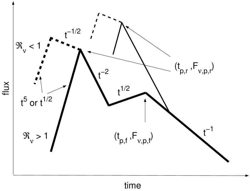
Figure 1.— Typical lightcurves of the reverse-forward shock emission combinations for the homogeneous ISM case. The thick lines depict a typical “rebrightening” (type I) lightcurve, while thin lines indicate a typical “flattening” (type II) lightcurve. The forward shock peak $(t_{p,f},F_{\nu,m,p})$ is defined at the transition point of the $\propto t^{1/2}$ to $\propto t^{-1}$ lightcurves. The reverse shock peak $(t_{p,r},F_{\nu,m,r})$ is defined at the beginning of the $\propto t^{-2}$ segment for the reverse shock emission. Before this point, the lightcurve is $\propto t^{5}$ (thin shell) or $\propto t^{1/2}$ (thick shell) for ${\cal R}_{\nu}\equiv\nu_{R}/\nu_{m,r}(t_{\times})>1$ (usually the case), and $\propto t^{-1/2}$ for ${\cal R}_{\nu}<1$.

References

- (1) Akerlof, C. W. et al. 1999, Nature, 398, 400
- (2) Baring, M. G. & Harding, A. K. 1997, ApJ, 491, 663
- (3) Chevalier, R. A. & Li, Z.-Y. 1999, ApJ, 520, L29
- (4) Coburn, W. & Boggs, S. E. 2003, Nature, 423, 415
- (5) Crew, G. et al. 2002, GCN 1734, (http://gcn.gsfc.nasa. gov/gcn/gcn3/1734.gcn3)
- (6) Fan, Y. Z., Dai, Z. G., Huang, Y. F. & Lu, T. 2002, ChJAA, 2, 449
- (7) Fox, D. W. 2002, GCN 1564 (http://gcn.gsfc.nasa.gov/gcn/gcn3/ 1564.gcn3)
- (8) Fox, D. W. & Price, P. A. 2002, GCN 1731 (http://gcn.gsfc.nasa. gov/gcn/gcn3/1731.gcn3)
- (9) Fox, D. W. et al. 2003, ApJ, 586, L5
- (10) Kennel, C. F., & Coroniti, F. V. 1984, ApJ, 283, 694
- (11) Kobayashi, S 2000, ApJ, 545, 807
- (12) Kobayashi, S, Piran, T & Sari, R. 1999, ApJ, 513, 669
- (13) Kobayashi, S, & Sari, R. 2000, ApJ, 542, 819
- (14) Kobayashi, S, & Zhang, B. 2003a, ApJ, 582, L75
- (15) —–. 2003b, ApJ, submitted (astro-ph/0304086)
- (16) Li, W., et al., 2002, GCN 1737 (http://gcn.gsfc.nasa.gov/gcn/gcn3/ 1737.gcn3)
- (17) Li, W., et al. 2003, ApJ, 586, L9
- (18) Lithwick, Y. & Sari, R. 2001, ApJ, 555, 540
- (19) Mészáros, P. & Rees,M.J. 1997a, ApJ, 476, 231
- (20) —–. 1997b, ApJ, 482, L29
- (21) —–. 1999, MNRAS, 306, L39
- (22) Panaitescu, A., & Kumar, P. 2001, ApJ, 560, L49
- (23) Park, H. S., Williams, G. & Barthelmy, S. 2002, GCN 1736
- (24) (http://gcn.gsfc.nasa. gov/gcn/gcn3/1736.gcn3)
- (25) Sari, R. 1997, ApJ, 489, L37
- (26) Sari, R. & Piran, T. 1995, ApJ, 455, L143
- (27) —–. 1999a, ApJ, 517, L109
- (28) —–. 1999b, ApJ, 520, 641
- (29) Sari, R., Piran, T. & Narayan, R. 1998, ApJ, 497, L17
- (30) Shirasaki, Y. et al. 2002, GCN 1565 (http://gcn.gsfc.nasa. gov/gcn/gcn3/1565.gcn3)
- (31) Soderberg, A. M., & Ramirez-Ruiz, E. 2002, MNRAS, 330, L24
- (32) Usov, V. V. 1992, Nature, 357, 472
- (33) Wang, X. Y., Dai, Z. G., & Lu, T. 2000, MNRAS, 319, 1159
- (34) Wei, D. M. 2003, A&A, 402, L9
- (35) Wheeler, J. C., Yi, I., Höflich, P. & Wang, L. 2000, ApJ, 537, 810
- (36) Wolzniak, P., et al. 2002, GCN 1757 (http://gcn.gsfc.nasa. gov/gcn/gcn3/1757.gcn3)
- (37) Zhang, B. & Mészáros, P. 2002a, ApJ, 571, 876
- (38) —–. 2002b, ApJ, 581, 1236
- (39)