Neutrinos From Individual Gamma-Ray Bursts in the BATSE Catalog

Abstract

We estimate the neutrino emission from individual gamma-ray bursts observed by the BATSE detector on the Compton Gamma-Ray Observatory. Neutrinos are produced by photoproduction of pions when protons interact with photons in the region where the kinetic energy of the relativistic fireball is dissipated allowing the acceleration of electrons and protons. We also consider models where neutrinos are predominantly produced on the radiation surrounding the newly formed black hole. From the observed redshift and photon flux of each individual burst, we compute the neutrino flux in a variety of models based on the assumption that equal kinetic energy is dissipated into electrons and protons. Where not measured, the redshift is estimated by other methods. Unlike previous calculations of the universal diffuse neutrino flux produced by all gamma-ray bursts, the individual fluxes (compiled at http://www.arcetri.astro.it/$\sim$ dafne/grb/) can be directly compared with coincident observations by the AMANDA telescope at the South Pole. Because of its large statistics, our predictions are likely to be representative for future observations with larger neutrino telescopes.

1 Introduction

The leading models for Gamma-Ray Bursts (GRB), bursts of 0.1-1 MeV photons typically lasting for 0.1-100 seconds (Fishman & Meegan 1995), involve a relativistic wind emanating from a compact central source. The ultimate energy source is rapid accretion onto a newly formed stellar mass black hole.

Observations suggest that the prompt $\gamma$-ray emission is produced by the dissipation (perhaps due to internal shocks) of the kinetic energy of a relativistically expanding wind, i.e. a “fireball”. Both synchrotron and inverse Compton emissions from the shock-accelerated electrons have been proposed as the GRB emission mechanism.

In this paper, we study in detail the production of neutrinos by protons accelerated along with electrons. We assume that equal energy of the fireball is dissipated in protons and electrons (or photons). This is the case in models where GRBs are the sources of the highest energy cosmic rays. The basic idea is that the protons produce pions decaying into neutrinos in interactions with the fireball photons, or with external photons surrounding the newly formed black hole.

Where previous calculations have estimated the universal diffuse flux of neutrinos produced by all GRBs over cosmological time, we estimate the flux from individual GRBs observed by the BATSE (Burst And Transient Source Experiment) experiment on the Compton Gamma-Ray observatory. The prediction can be directly compared with coincident observations performed with the AMANDA detector. Having these observations in mind, we specialize on neutrino emission coincident in time with the GRB. Opportunities for neutrino production exist after and, in some models, before the burst of $\gamma$-rays, e.g. when the fireball expands through the opaque ejecta of a supernova.

The calculations are performed in two models chosen to be representative and rather different versions of a large range of competing models. The first is generic for models where an initial event, such as a merger of compact objects or the instant collapse of a massive star to a black hole, produces the fireball (Waxman & Bahcall 1997 ;Guetta, Spada & Waxman 2001a, GSW hereafter). We calculate the neutrino production by photomeson interactions of relativistic protons accelerated in the internal shocks and the synchrotron photons that are emitted in these shocks. The neutrinos produced via this mechanism have typical energies of $\sim 10^{14}-10^{15}$ eV, and are emitted in coincidence with the GRBs, with their spectrum tracing the GRB photon spectrum. For an alternative model, we have chosen the supranova model where a massive star collapses to a neutron star with mass $\sim 2.5-3\,M_{\odot}$, which loses its rotational energy on a time scale $t_{\rm sd}$ of weeks to years, before collapsing to a black hole, thus triggering the GRB. Following Guetta and Granot (Guetta & Granot 2002a), we calculate the neutrino flux from interactions of the fireball protons with external photons in the rich radiation field created during the spindown of the supra-massive pulsar. Production on external photons turns out to be dominant for a wide range of parameters, $t_{\rm sd}\lesssim 0.2\;$yr for a typical GRB and $t_{\rm sd}\lesssim 2\;$yr for X-ray flashes. The neutrinos produced via this mechanism have energies $\varepsilon_{\nu}\sim 10^{15}-10^{17}\,(10^{19})\;$eV for typical GRB (X-ray flashes) and are emitted simultaneously with the prompt $\gamma$-ray (X-ray) emission. Their energy spectrum consists of several power law segments and its overall shape depends on the model parameters, especially $t_{\rm sd}$. If the mass of the supernova remnant is of the order of $\sim 10M_{\odot}$, and if the supernova remnant shell is clumpy, then for time separation $t_{\rm sd}<0.1$ yr the SNR shell has a Thomson optical depth larger than unity and obscures the radiation emitted by the GRB. Therefore, for $t_{\rm sd}\lesssim 0.1\;$yr, the $\nu$’s would not be accompanied by a detectable GRB providing us with an example of neutrino emission not coinciding with a GRB display.

As previously mentioned, to realistically estimate the neutrino fluxes associated with either of these models, we turn to the GRB data collected by BATSE. The BATSE records include spectral and temporal information which can be used to estimate neutrino spectra for individual bursts. We will perform these calculations for two version of each of the two models previously described. The two versions correspond to alternative choices of important parameters. The wide variety of GRB spectra results, not surprisingly, in a wide range of neutrino spectra and event rates. For approximately 800 bursts in the BATSE catalog, and for four choices of models, we have calculated the neutrino spectra and the event rates, coincident with GRBs, for a generic neutrino telescope. With 800 bursts, the sample should also be representative for data expected from much larger next-generation neutrino observatories.

Neutrino telescopes can leverage the directional and time information provided by BATSE to do an essentially background-free search for neutrinos from GRBs. Individual neutrino events within the BATSE time and angular window are a meaningful observation. A generic detector with 1 km² effective telescope area, during one year, should be able to observe 1000 bursts over $4\pi$ steradians. Using the BATSE GRBs as a template, we predict order 10 events, muons or showers, for both models. The rates in the supranova model depend strongly on $t_{\rm sd}$. In this model we anticipate $\sim 7$ events per year assuming $t_{\rm sd}\simeq 0.07$ yr, but only one event per ten years for $t_{\rm{sd}}\simeq 0.4$ yr. We will present detailed tabulated predictions further on. They can be accessed at http://www.arcetri.astro.it/$\sim$dafne/grb/.

Short duration GRBs, characterized by lower average fluences, are less likely to produce observable neutrino fluxes.

We find that GRBs with lower peak energies, X-ray flash candidates, yield the largest rates in the supranova model. For instance, for $t_{\rm{sd}}\simeq 0.07$ yr, we predict one event (muon or shower) for every 1000 bursts. If only 100, or so, X-ray flashes occur per year, as observations suggest, this will be difficult to observe. However, such events may be considerably more common and may contribute significantly to the diffuse high energy neutrino flux. Observations of neutrinos from this class of GRBs would be strong evidence for a supranova progenitor model.

The AMANDA collaboration has collected neutrino data in coincidence with BATSE observations (Barouch & Hardtke 2001). It operated the detector for 3 years (1997-1999) with an effective area of approximately 5,000 m² for GRBs events. In early 2000 the expanded detector reached an effective area of roughly 50,000 m². Unfortunately, only $\sim$ 100 coincident bursts could be observed with the completed detector before BATSE operations ceased in June 2000. With effective areas significantly below the canonical square kilometer discussed in this paper, AMANDA is not large enough to test the GRB models considered here. We estimate only 0.08 events in 1997-1999 and 0.3 in 2000.

Our estimate of 1–10 events in 1 year for a telescope with 1 kilometer square telescope area is consistent with previous, burst-averaged, determinations of the GRB neutrino flux (Alvarez, Halzen & Hooper 2000, Dermer & Atoyan 2003). Note that the effective area of IceCube for GRB will significantly exceed this reference value (PDD). The rate can be understood by a back-of-the-envelope estimate. A typical GRB produces a photon fluence on the order of $10^{-5}\,\rm{ergs}/\rm{cm}^{2}$, which we assume to be equal to the energy in protons. If $20\%$ of the proton energy is converted into pions, half to charged pions, and one quarter of the charged pion energy to muon neutrinos in the $\pi\rightarrow\mu\rightarrow e$ decay chain, then $\sim 5\times 10^{-7}\,\rm{ergs}/\rm{cm}^{2}/E_{\nu}$ neutrinos are generated. For a typical neutrino energy of $E_{\nu}\sim 100\,\rm{TeV}$, this yields $\sim 30$ neutrinos per square kilometer. At this energy the probability that a neutrino converts to a muon within range of the detector is $10^{-4}$ (Gaisser, Halzen, Stanev 1995). Therefore $3\times 10^{-3}\,$ muons are detected in association with a single GRB. With over 1000 GRBs in one year, we estimate a few muons per year in a kilometer-square detector. Fluctuations in fluence and other burst characteristics enhance this estimate significantly (see Figure 2, for instance), however, absorption of neutrinos in the Earth can reduce this number. These effects are included in the calculations of actual event rates throughout this paper.

Our estimates, while observable with future kilometer-scale observatories, may be conservative. We already mentioned bursts with no counterpart in photons. Also, occasional nearby bursts, much like supernova, could exceptionally provide higher event rates than our calculations reflect. We would like to point out the fact that the aim of the paper is not to do more precise calculations than the ones already done in the literature. We just want to generate results that can be compared with experiments that do coincidents observations with satellites.

The outline of the paper is somewhat unconventional. The detailed results are collected in a data archive at http://www.arcetri.astro.it/$\sim$dafne/grb. The details of the calculations of the neutrino fluxes in the two models are described in appendices A and B. In appendix C we collected the methods used to evaluate the rates of neutrino-induced muons, taus and showers in a generic detector with a given effective telescope area. The main body of the paper is organized as follows. In §2, we review GRB models and describe the mechanisms for neutrino production in GRBs. In §3 and §4 we describe the BATSE catalog of GRBs and we identify subclasses of events: long duration GRBs with and without measured redshift, short duration GRBs and X-ray flash candidates. In §5 we summarize our simulation of the response of a generic high energy neutrino telescope to the predicted neutrino fluxes. In §6 we analyse some anomalous bursts. Results and conclusions are collected in §7.

2 GRB Models and Neutrino Emission

Progenitor models of GRBs are divided into two main categories. The first category involves the merger of a binary system of compact objects, such as a double neutron star (Eichler et al. 1989), a neutron star and a black hole (Narayan, Pacyński & Piran 1992) or a black hole and a Helium star or a white dwarf (Fryer & Woosley 1998; Fryer, Woosley & Hartmann 1999). The second category involves the death of a massive star. It includes the failed supernova (Woosley 1993) or hypernova (Pacyński 1998) models, where a black hole is created promptly, and a large accretion rate from a surrounding accretion disk (or torus) feeds a strong relativistic jet in the polar regions. This type of model is known as the collapsar model. An alternative model within this second category is the supranova model (Vietri & Stella 1998), where a massive star explodes in a supernova and leaves behind a supra-massive neutron star (SMNS), of mass $\sim 2.5-3\,M_{\odot}$. It subsequently loses its rotational energy on a time scale $t_{\rm sd}$ of order weeks to years until it collapses to a black hole. This triggers the GRB. Long GRBs (with a duration $\gtrsim 2\;{\rm s}$) are usually attributed to the second category of progenitors, while short GRBs are attributed to the first category.

We select two models to investigate the opportunities for neutrino production in a GRB. The analysis can be easily extended to other models (see for example Razzaque, Mészáros & Waxman 2002; Dermer & Atoyan 2003). The first model is based on the standard fireball phenomenology where electrons and protons are shock accelerated in the fireball. Pions and neutrinos are produced by photoproduction interactions when the protons coexist in the fireball with photons. These are produced by synchrotron radiation of accelerated electrons. For a second model we turn to the supranova scenario where the supra-massive pulsar loses its rotational energy through a strong pulsar wind. This pulsar wind creates a rich external radiation field before the collapse to the final black hole and the creation of the GRB fireball. It is referred to as the pulsar wind bubble (PWB) (Königl & Granot 2002; Inoue, Guetta & Pacini 2002; Guetta & Granot 2003) and provides a target for the photoproduction of neutrinos by fireball protons. Let’s note in passing that the supranova model has several advantages compared to other collapsar models: (i) the jet does not have to penetrate the stellar envelope (Vietri & Stella 1998), (ii) it can naturally explain the X-ray line features observed in several afterglows (Piro et al. 2000; Lazzati, et al. 2001; Vietri et al. 2001), and (iii) the large fraction of the internal energy in the magnetic field and in electrons observed in the afterglow emission arise naturally (Königl & Granot 2002; Guetta & Granot 2003).

In all of the different scenarios mentioned above, the final stage of the process consists of a newly formed black hole with a large accretion rate from a surrounding torus, and involve a similar energy budget ($\lesssim 10^{54}\;{\rm ergs}$). Observations suggest that prompt $\gamma$-ray emission is produced by the dissipation of the kinetic energy within the fireball, due to internal shocks within the flow that arise from variability of the Lorentz factor, $\Gamma$, on a time scale $t_{v}$. The afterglow emission is thought to arise from an external shock that is driven into the ambient medium as it decelerates the ejected matter (Rees & Mészáros 1994; Sari & Piran 1997). In this so called ‘internal-external’ shock model, the duration of the prompt GRB is directly related to the time during which the central source is active. The emission mechanism is successfully described by synchrotron radiation from relativistic electrons that radiate in the strong magnetic fields. These are close to equipartition values within the shocked plasma. An additional radiation mechanism that may also play some role is synchrotron self-Compton (SSC) (Guetta & Granot 2002b), which is the upscattering of the synchrotron photons by relativistic electrons to higher energy.

Protons are expected to be accelerated along with the electrons in the region where the wind kinetic energy is converted into internal energy due to a dissipation mechanism like internal shocks. The conditions in the dissipation region allow proton acceleration up to $\varepsilon_{p,{\rm max}}\gtrsim 10^{20}\;$eV (Waxman 1995; Vietri 1995). The energy in $\gamma$-rays reflect the fireball energy in accelerated electrons and afterglow observations indicate that accelerated electrons and protons carry similar energy (Freedman & Waxman 2000). Our basic assumption in calculating neutrino emission from GRBs is that equal amounts of energy go into protons and photons. In models where GRB protons are the source of the highest energy cosmic rays, this assumption is supported by the approximate equality of the $\gamma$-ray fluence of all GRBs and the total energy in extragalactic cosmic rays.

Both internal shocks, responsible for the prompt GRB emission, and the external shock, responsible for the afterglow emission, have been proposed as possible sources of the highest energy cosmic rays (Waxman 1995 and Vietri 1995, respectively). A comparison between the two mechanisms has been done by Vietri, De Marco and Guetta (2003), but it is not easy to conceive, at this point, an observational test capable of distinguishing between the two models. The only hope appears to observe the production of high energy neutrinos which must accompany the in situ acceleration of particles. Occasionally, ultra-high energy protons will produce pions and neutrinos in collisions with photons in photon rich environment provided by the post–shock shells or by the pulsar wind bubble. If the protons are accelerated in internal shocks, the neutrinos produced will arrive at Earth simultaneously with the photons of the burst proper and will have an energy $\sim 10^{15}-10^{16}\,\rm{eV}$ (Waxman and Bachall 1997; GSW; Guetta & Granot 2002a). If accelerated in external shocks, they will arrive at Earth simultaneously with the photons of the afterglow and will have a higher energy, $\gtrsim 10^{17}$ eV (Vietri 1998a, 1998b, Waxman & Bahcall 2000).

General phenomenological considerations indicate that gamma-ray bursts are produced by the dissipation of the kinetic energy of a relativistic expanding fireball. Internal shocks that are mildly relativistic are believed to dissipate the energy. Therefore, the proton energy distribution should be close to that for Fermi acceleration in a Newtonian (non-relativistic) shock, $dn_{p}/d\varepsilon_{p}\propto\varepsilon_{p}^{-2}$. Moreover, the power law index of the electron and proton energy distributions are expected to be the same, and the values inferred for the electron distribution from the observed photon spectrum are $dn_{e}/d\varepsilon_{e}\propto\varepsilon_{e}^{-p}$ with $p\sim 2-2.5$. We shall, therefore, adopt $dn_{p}/d\varepsilon_{p}\propto\varepsilon_{p}^{-2}$. Plasma parameters in the dissipation region allow proton acceleration to energies greater than $10^{20}$ eV (Waxman 1995, Vietri 1995).

We will assume that the fireball is spherically symmetric. Note, however, that a jet-like fireball behaves as if it were a conical section of a spherical fireball as long as $\theta_{j}>1/\Gamma$, where $\theta_{j}$ is the jet opening angle and $\Gamma\gtrsim 300$ is the wind Lorentz factor. Therefore, our results apply without modification to a jet-like fireball. For a jet-like wind, the luminosity, $L$, in our equations should be understood as the luminosity of the fireball inferred by assuming spherical symmetry.

We have relegated all details of the calculation of neutrino production via photomeson interaction with GRB photons and PWB photons to appendices A and B, respectively. Throughout the paper, we will refer to the models by the following convention:

• Model 1: Neutrino flux from the interaction of high-energy protons with GRB photons. The fraction of proton energy transfered to pion energy is set to 0.2 as indicated by simulations of GSW (see apppendix A).

• Model 2: Neutrino flux from the interaction of high-energy protons with GRB photons. The fraction of proton energy transfered to pion energy is calculated as described in appendix A (see appendix A).

• Model 3: Neutrino flux from the interaction of high-energy protons with PWB photons, as in the supranova progenitor model. The time scale between supernova and GRB is set to $t_{\rm{sd}}=0.4$ yr (see appendix B).

• Model 4: Neutrino flux from the interaction of high-energy protons with PWB photons, as in the supranova progenitor model. The time scale between supernova and GRB is set to $t_{\rm{sd}}=0.07$ yr (see appendix B).

3 The BATSE Catalog

BATSE, the Burst And Transient Source Experiment, was a high energy astrophysics experiment launched on the Compton Gamma-Ray Observatory in 1991. BATSE, between its launch and the termination of its orbit in 2000, has observed and recorded data from over 8000 events including gamma-ray bursts, pulsars, terrestrial gamma-ray flashes, soft gamma repeaters and black holes.

The data BATSE recorded from gamma-ray bursts is publically available in the current BATSE catalog at http://f64.nsstc.nasa.gov/batse/grb/catalog/. For a description see Paciesas et al. 1999. The catalog includes information on the spectrum, time and location of each triggered burst. Each triggered event has been assigned a BATSE trigger number (between 105 and 8121 for GRBs) which we use to identify individual bursts.

Spectral information is recorded in four energy channels, 20-50 keV, 50-100 keV, 100-300 keV and above 300 keV. Using these four fluence measurements, we have fitted the spectrum of each GRB to a broken power law, treating the break energy, both spectral slopes and the normalization as free parameters; see Eq.(A6). We determine the Lorentz factor of the relativistic expanding ejecta using the break energy through Eq.(A18). For bursts with an observed break energy above 300 keV, or below 50 keV, it is difficult to determine both the break energy and the power law slope. For high energy breaks, the impact on this ambiguity is not critical. As explained in appendix A, the Lorentz factor is not dependent on the fit because it is fixed by the observed high energy of the event and the requirement that the fireball be optically thin. For very low spectral breaks (below 50 keV), for instance in events we classify as X-ray flash candidates, we acknowledge a significant degree of uncertainty in the Lorentz factor calculation and resulting neutrino spectra. In this case, the spectral break is only uncertain to about a factor of 2 or 3.

Detailed temporal information is available in the BATSE catalog, in the form of light curves. The BATSE time resolution varies between 2.048 seconds and 0.016 seconds. A resolution of 0.064 seconds is available for all bursts during the time following the trigger.

In the framework of the internal shock model, we need a variability time, $t_{v}$, $\lesssim 0.01s$ in order to get the 1MeV $\gamma-rays$ (Guetta, Spada & Waxman 2001b, Waxman 2001). In fact with a value of the Lorentz factor larger than the minimal value needed to be optically thin up to 100 Mev ($\sim 250$ see Eq.A17) the variability time, $t_{v}$, has to be $\lesssim 10ms$ to get the 1 MeV $\gamma$-rays.

How well the data support the model is still controversial and a detailed analysis on this issue is out of the aim of our paper. Since we refer to this model for our analysis we consider a value of $t_{v}=10$ ms for long duration GRBs in the rest of the paper. For short duration bursts we take $t_{v}=0.1$ ms and 0.050 seconds for X-ray flash candidates.

4 GRB Classes

We have divided the list of BATSE GRBs into four different classes: 1) long duration bursts (duration $\gtrsim 2\;{\rm s}$) with measured redshfit, 2) long duration bursts without measured redshift, 3) short duration bursts and 4) X-ray flashes. Major differences in temporal and spectral properties of long duration GRBs, short duration GRBs and X-ray flashes has lead to some speculation that they may involve different progenitors or mechanisms.

4.1 Long Duration GRBs With Measured Redshift

By observing the optical afterglow of GRBs, it is possible to measure spectral lines and, therefore, the redshift of an individual burst. Although to date the X-ray afterglow of on the order of 100 long duration GRBs have been observed, only 31 of them have been observed in the optical making a determination of the redshift possible. (No redshift has been identified for short GRBs). We first consider 13 of these that have a complete BATSE record.

The relationship between the comoving distance to an object and its redshift is given by:

$$d=\frac{c}{H}\int^{z}_{0}\frac{dz^{\prime}}{\sqrt{\Omega_{\Lambda}+\Omega_{\rm{M}}(1+z^{\prime})^{3}}}$$ (1)

Where $\Omega_{\Lambda}\simeq 0.7$ and $\Omega_{\rm{M}}\simeq 0.3$ are the fractions of the critical density of the Universe in dark energy and matter, respectively. $H$ is Hubble’s constant.

Once the distance to a GRB is known, and its fluence (or flux) has been measured, the isotropic-equivalent $\gamma$-ray luminosity can be calculated. From this and the value of $t_{v}=0.01\;\rm{s}$, together with the break energy of the GRB photon spectrum, we estimate the bulk Lorentz factor using Eqs.(A17, A18). Setting the efficiency for pion production $f_{\pi}=0.2$ for model 1 and using Eq.(A16) for model 2, we estimate the fraction of proton energy transfered into pions. Using Eqs.(A10, A11) the energy scale of synchrotron losses, $\varepsilon^{\rm{s}}_{\nu}$, is determined. From these informations we can determine the neutrino flux at Earth for each of the four models. For a more detailed discussion see appendices A and B.

4.2 Long Duration GRBs Without Measured Redshift

For the majority of the long duration bursts in the BATSE catalog no redshift is available. In this case, the $\gamma$-ray luminosity of long duration bursts, and, therefore, the distance, can be estimated by assuming a relationship between the observed variability and the luminosity of a GRB (Lloyd-Ronning & Ramierz-Ruiz 2002; Zhang & Meszaros 2002; Kobayashi, Ryde & MacFadyen 2002). Note that the variability of a GRB is not the same as its variability time, $t_{v}$, previously introduced.

The variability of burst is a measure of fluctuations in the temporal structure of the burst. It is defined such that pure noise should have a variability of zero, while the most variable bursts have very sudden and distinctive temporal features. We use the following definition of variability (Fenimore & Ramirez-Ruiz 2000):

$$V=Y^{-0.24}\frac{1}{N}\Sigma\frac{(F_{i}-F_{{0.30}\times{T_{90}}})^{2}-(F_{i}+B)}{F^{2}_{\rm{peak}}}$$ (2)

where $Y=(1+z)/3$, $F_{i}$ is the background subtracted fluence in a time bin $i$, $B$ is the average background in a single time bin, $F_{\rm{peak}}$ is the maximum fluence and $F_{{.30}\times{T_{90}}}$ is the average fluence over a time period centered at time bin $i$ of length 30% of the $T_{90}$ time (duration) of the burst.

The GRBs with observed redshifts have been used to empirically derive a relationship between the variability and the luminosity of the burst (Fenimore & Ramirez-Ruiz 2000; Reichart et al. 2001, Reichart & Lamb 2001):

$$L/d\Omega=3.1\times 10^{56}V^{3.35}\rm{erg}\,\,\rm{s}^{-1}.$$ (3)

A relationship between luminosity and the time lag between the peaks for light curves in different energy bands, has been observed in the GRB redshift data (Norris, Marani & Bonnell 2000), but appears to be less reliable. Therefore, we will only consider the luminosity-variability relationship.

Together with the fluence (flux) of a burst, the distance of a burst can be determined by the luminosity. Note that the variability, and therefore luminosity, of a burst depends on the redshift or distance to the burst. Therefore, we must do this calculation by iteration. The end result is a value of the luminosity and redshift for each burst. We would like to enphasize the fact that there are a lot of uncertainties in this way to estimate the redshift, however the knoweledge of the redshift is not so important in our analysis since the minimum variability time scales and the fluence are the most important quantities.

It is difficult to reliably calculate the variability of bursts with low flux. For this reason, we only consider bursts with a peak flux greater than 1.5 photons/$\rm{cm}^{2}\rm{sec}$ (over a 0.256 s time scale) and with at least 30 time bins (of 0.064 s width) of 5 sigma or more above the average background. The GRBs which do not meet these requirements have low fluence and are therefore likely to yield a low neutrino flux anyway. After these criteria were applied, 566 long duration bursts without measured redshift are left, making it our largest class.

Even for bursts which meet the above criteria, the luminosity estimated is only accurate to an order of magnitude. This corresponds to uncertainties of a factor of 2 or 3 in the fraction of proton energy transfered into pions and in the synchrotron loss energy.

4.3 Short Duration GRBs

Short duration GRBs, with no observation of an optical afterglow and, therefore, no measurement of redshift, cannot have a relationship between variability and luminosity empirically established. Additionally, variability is difficult to measure for short duration bursts. Left with no way to measure the $\gamma$-ray luminosity of, or distance to, a short duration GRBs, we choose to set $z=1$ for each burst. This introduces greater uncertainty than in the long duration GRBs case but, given the ambiguities in the burst characteristics, it is the best that can be done at this time. To be consistent, we considered only short bursts with a peak flux greater than 1.5 photons/$\rm{cm}^{2}\rm{sec}$ (over a 0.256 s time scale), as we did with for long duration GRBs. After this criteria was applied, 199 short duration bursts remained in this category.

Temporal structure and variations appear to occur on shorter time scales for short compared to long GRBs (McBreen et al. 2002). We therefore use a time scale of temporal fluctuations of $t_{v}=0.001\,\rm{s}$ for all short duration bursts, as opposed to the value of $t_{v}=0.01\,\rm{s}$ used for long duration bursts. It is also interesting to note that short duration bursts generally have a somewhat harder spectrum and higher peak energy than long duration GRBs (Paciesas et al. 2001).

4.4 X-Ray Flash Candidates

X-ray flashes are a newly discovered class of fast transient sources. The BeppoSAX experiment’s wide field cameras have observed such events at a rate of about four per year (Heise et al. 2001, Kippen et al. 2002), implying a total rate on the order of $100$ per year. These events typically have peak energies as low as 2-10 keV and durations of 10-100 seconds. The BeppoSAX experiment discriminates X-ray flashes from standard GRBs by the non-detection of a signal above 40 keV with the BeppoSAX GRB monitor. More generally, a large ratio of X-ray to $\gamma$-ray fluence is the differentiating characteristic of X-ray flashes from GRBs. It has been suggested, however, that X-ray flashes are a low peak energy extension of gamma-ray bursts (Heise et al. 2001, Kippen et al. 2002).

The final class considered here consists of BATSE events which may be X-ray flashes. We identify 15 events in this class with spectra that peak below 50 keV, although it is difficult to determine accurately where the peak occurs because the sensitivity of BATSE is somewhat poor in this energy range. These are long duration bursts, and typically have a hard spectrum; several have $\beta$ in Eq.(A6) larger than 1.5, and no observed flux in BATSE’s fourth energy channel (above 300 keV).

Again, with no measured redshift, and limited temporal information, we cannot deduce the luminosities of these events. We set $z=1$ for each event and calculate its luminosity accordingly. It is thought that the radius of collisions in X-ray flashes is typically larger than in other GRBs and, therefore, the time scale of fluctuations will generally be larger (Guetta, Spada & Waxman 2001b). We therefore choose $t_{v}=0.05\,\rm{s}$. For some X-ray flashes the peak energy is very low (20-30 keV) and the Lorentz factor accordingly very high. Increasing the time scale of fluctuations has the additional effect of lowering the Lorentz factor to a reasonable value in these extreme cases (see Eq.(A18)).

For X-ray flashes, with a very large Lorentz factor and a long time scale of fluctuations, we expect that a very small fraction of proton energy converted to pions; see Eqs.(A15,A16). We therefore expect low neutrino fluxes from proton interactions with GRB photons. For the models involving proton interactions with photons in a surrounding pulsar wind bubble, however, the rates can be quite high (Guetta & Ganot 2002a).

There is another class of objects that are the non-triggered bursts. They are found in the BATSE data in off-line analysis; see e.g. Stern and Tikhomirova
(http://www.astro.su.se/groups/head/grb_-archive.html). They are not energetic enough to trigger in real time. These can be GRBs with low kinetic luminosity and will be very weak neutrino sources for all the four models, therefore we have decided to neglect them in our analysis.

4.5 Neutrino GRB Database

We have constructed a database publicly accessible online with a complete list of all of the GRB characteristics and associated neutrino event rates for the approximately 800 bursts we have considered in this analysis. The data was populated in a MySQL database, interacting through a user-friendly web interface developed with PERL. The database is searchable by GRB number and/or by GRB class, and is capable of searching for only bursts included in the AMANDA analysis or all bursts in this work. The rates are for a generic neutrino telescope provided the threshold is sufficiently low for observing the neutrino fluxes predicted. How we transform the GRB neutrino fluxes into observed event rates is the topic of the next section. Representative results are tabulated in tables 1 through 12. The database also contains the predicted neutrino spectra for each burst; these can be directly combined with the simulation of a specific detector. The database is accessible at http://www.arcetri.astro.it/$\sim$dafne/grb.

5 Neutrino Telescopes and Event Simulation

Large volume neutrino telescopes are required to observe and measure the neutrino flux from GRBs. Current experiments, such as AMANDA (Andres et al. 2001) at the South Pole, or future (Aslanides et al. 1999) and next generation experiments, including IceCube (see http://icecube.wisc.edu/) with a full cubic kilometer of instrumented detector volume, i.e. with $>1{\rm km^{2}}$ telescope area, are designed to observe high energy cosmic neutrinos with energies expected from GRBs.

Neutrino telescopes detect the Cherenkov light radiated by showers (hadronic and electromagnetic), muons, and taus that are produced in the interactions of neutrinos inside or near the detector. Muons are of particular interest because, at the energies typical for GRB neutrinos, they travel kilometers before losing energy. The dominant signal is, therefore, through-going muons. IceCube can measure the energy and direction of any observed muon. The angular resolution is less than $1^{\circ}-3^{\circ}$ while the energy resolution is approximately a factor of three. Signal and background muons may, therefore, be differentiated with a simple energy cut. For shower events the energy measurement improves significantly, being better than 20%, but reconstructing their direction is challenging, the angular resolution being of order 10 degrees.

For high energies, when tau decay is sufficiently time dilated, taus have a range similar to or larger than muons, and so the dominant tau signal is from through-going taus. These events have a characteristic signature consisting of a “clean” minimum-ionizing track despite its long range inside the detector. We will therefore consider all events in which a tau track passes through the detector in the direction and at the time of a GRB. We assume that taus and muons are distinguishable at all energies when specializing to rare events in coincidence in time and direction with a GRB. We realize that, in general, it may be difficult to distinguish a muon of energy $\lesssim 200$ GeV, that is expected to lose relatively little energy from catastrophic processes, from a very high energy tau. Tau signatures however become dramatic when they decay inside the detector (lollipop events), or when the tau neutrino interacts and the produced tau decays into showers inside the detector (double bang events).

To evaluate the prospects for GRB neutrino observations, it is essential to determine the rate of muon, shower and tau events. These calculations are each described in appendix C. For a review of high energy neutrino astronomy; see (Halzen & Hooper 2002; Learned & Mannheim 2000).

6 Anomalous Bursts

There are a few GRBs we have considered in this analysis which are anomalous for a variety of reasons. We briefly mention these in this section.

• GRB 6707 is a burst with a measured redshift of 0.0085, yet a relatively low fluence of $4\times 10^{-6}\,\rm{erg}/\rm{cm}^{2}$. Together, this implies a luminosity on the order of $10^{45}\,$erg/s, well below the normal range considered. Our calculation of the Lorentz factor, which depends on the luminosity of the GRB, yields a value of about 25,000, much larger than the normally allowed range. Results in model 2 are, therefore, not particularly realistic for this particular burst (the rates are actually very low for this model). The other models are only affected by this in the calculation of the synchrotron energy loss scale.

• GRBs 7648, 6891 and 1997 each have Lorentz factors below 100. In all three cases, the burst has been found to have a low luminosity, $\sim 10^{49}\,$erg/s, which contributes to this result. The results of models 2, 3 or 4 are only affected by this in their low synchrotron energy loss scales, and are, therefore, conservative. Results for model 1 should be interpreted with caution for these three GRBs.

• GRBs 1025 and 8086, both long duration bursts, have been found to have very low variabilities and, therefore, low luminosities. This results in very high Lorentz factors in our calculation (20,000 and 5,000, respectively). Given the uncertainties involved in the variability calculation and the variability-luminosity relationship, we feel that these luminosities and Lorentz factors are unlikely to accurately represent these bursts.

7 Results and Discussion

As already mentioned, our results are summarized in a series of tables. They summarize our fits to the BATSE data that provide the input spectrum for calculating the neutrino emission. The neutrino event rates for the 4 classes and the 4 models are also tabulated (see tables 1 through 8). In tables 9-12, we summarize the event rates for a generic kilometer-scale telescope, such as IceCube, for the 4 classes of GRBs. For the duration and in the direction of a GRB, the background in a neutrino telescope should be negligible. Therefore individual events represent a meaningful observation when coincident with a GRB. We next evaluate the prospects for such observations.

The AMANDA experiment has operated for approximately four years (1997-2000) that overlap with the BATSE mission (Barouch & Hardtke 2001). Data has been collected for several hundred GRBs with an effective telescope area of order 5,000 m² . AMANDA-II, the completed version of the experiment, with approximately 50,000 m² effective area for the high energy neutrinos emitted by GRBs, was commissioned less than half a year before the end of the BATSE mission. Nevertheless, of order 100 bursts occurred during that period for which coincident observations were made. With effective areas significantly below the reference square kilometer of future neutrino telescopes, AMANDA is not expected to test the GRB models considered here. For long duration GRBs, the most common classification, we anticipate on the order of 0.01 events (muons+showers) per square kilometer per GRB for models 1 and 2. For AMANDA-II, with one twentieth of this area, and only capable of observing northern hemisphere GRBs ($\sim 500$/yr), we predict on the order of .3 events (muons+showers) per year of observation. AMANDA-B10, with smaller area, should observe one tenth of this rate. It is interesting, however, to note that such experiments are on the threshold of observation at this time. IceCube with a square kilometer of effective area, now under construction, will likely cross this threshold.

For the high energies considered here, IceCube should be able to make observations of 1000 bursts over $4\pi$ steradians during one year. Where models 1 and 2 are concerned, we expect that an event (muon or shower) will be observed from roughly 10 GRBs. For models 3 and 4 we predict $\sim 7$ events per year for models with $t_{\rm{sd}}\simeq 0.07$ yr (model 4) , but only around one event per ten years if $t_{\rm{sd}}$ is somewhat larger, such as 0.4 yr (model 3). The prospects for observation depends strongly on $t_{\rm{sd}}$, as expected.

We expect that classes of GRBs with lower average fluence, such as short duration GRBs and X-ray flash candidates, will be more difficult to observe. X-ray flash candidates, although unlikely to be observable in models 1 and 2, could possibly be observed in models 3 and 4. If $t_{\rm{sd}}\simeq 0.07$ yr (model 4), we predict order one event (muon or shower) for every 1000 bursts. With only $\sim 100$ X-ray flashes thought to occur per year, such an observation will be unlikely. If such events are more common, however, they may contribute significantly to the diffuse high energy neutrino flux. Observations of neutrinos from low peak energy GRBs would be strong evidence for a supranova progenitor model.

It is interesting to note that the majority of the neutrino events from GRBs come from a relatively small fraction of the GRB population (Alvarez, Halzen & Hooper 2000; Halzen & Hooper 1999). In Figure 1 we show some of the factors which go into this conclusion. The occasional nearby (low redshift), large $f_{\pi}$, high fluence and/or near horizontal burst can dominate the event rate calculation. The distribution of the number of events per burst (or X-ray flash candidate) is shown in Figure 2.

In summary, taking advantage of the large body of GRB statistics available in the BATSE catalog, we have attempted to estimate the neutrino fluxes and event rates in neutrino telescopes associated with GRBs for a variety of theoretical models. Our analysis has yielded several conclusions:

• Gamma-ray bursts with high fluence, most often long duration bursts, provide the best opportunity for neutrino observations.

• For typical gamma-ray bursts, proton interactions with fireball photons provides the largest neutrino signal. We have also shown that the rates are relatively model independent.

• For gamma-ray bursts with very low peak energies, possibly associated with X-ray flashes, very little energy is transfered into pions (and, therefore, neutrinos) in interactions with fireball photons. Interactions with a surrounding pulsar wind bubble, however, can yield interesting neutrino fluxes. This is an illustration that observation of neutrinos is likely to help decipher the progenitor mechanism.

• While our calculations indicate that existing neutrino telescopes, such as AMANDA, are not likely to have the sensitivity to observe gamma-ray burst neutrinos, next generation, kilometer-scale observatories, such as IceCube, will be capable of observing on the order of ten bursts each year.

Table 1: Characteristics for GRBs with redshifts measured from optical afterglow observations. The fluence and zenith angle of each burst are taken from the BATSE catalog, whereas the luminosity is derived from the redshift and fluence. The break energy is obtained by a fit to the BATSE data and the Lorentz factor is calculated as described in Appendix A. Note that GRB 6707 is an anomalous burst (see §6).

BATSE $\#$	$F_{\gamma}$(erg/$\rm{cm}^{2}$)	$L_{\gamma}$(erg/s)	$z$	$E_{\gamma}^{b}$(MeV)	$\Gamma$	$\theta_{z}$ (degrees)
8079	$1.61~{}10^{-6}$	$4.9~{}10^{51}$	1.118	0.460	222.	166.2
7906	$2.51~{}10^{-4}$	$2.0~{}10^{52}$	1.020	1.460	281.	100.9
7648	$5.83~{}10^{-6}$	$2.0~{}10^{49}$	0.434	0.710	89.	101.8
7560	$2.06~{}10^{-5}$	$2.0~{}10^{51}$	1.619	0.100	925.	9.8
7549	$2.11~{}10^{-4}$	$1.2~{}10^{51}$	1.300	1	176.	63.8
7343	$4.87~{}10^{-4}$	$4.0~{}10^{51}$	1.600	0.280	214.	132.3
6891	$6.22~{}10^{-5}$	$1.5~{}10^{49}$	0.966	0.280	85.	102.0
6707	$4.01~{}10^{-6}$	$1.3~{}10^{45}$	0.009	0.430	25299.	36.9
6533	$1.25~{}10^{-5}$	$2.0~{}10^{52}$	3.420	0.460	281.	156.2
6225	$3.96~{}10^{-6}$	$1.2~{}10^{50}$	0.835	1.400	119.	170.6

Table 2: Estimated neutrino event rates for GRBs with redshifts measured from optical afterglow observations. Rates for muon and shower events are shown for the IceCube neutrino telescope. Tau events are not shown. Note that GRB 6707 is an anomalous burst. Model 1 and model 2 correspond to the internal shock scenario. In model 1 we fix the fraction of energy transferred from protons to pions to a constant value $f_{\pi}=20\%$, and in model 2 we calculate $f_{\pi}$ from the observed GRB characteristics using Eq.(A16). Models 3 and 4 correspond to the supranova scenario, with choices of the relevant parameter $t_{\rm sd}=0.4$ and 0.07 years respectively. Note that in the supranova scenario (models 3 or 4), internal shock processes (models 1 or 2) also contribute to the event rate. The total predicted rate for models 3 or 4 is, therefore, the sum of rates shown for the supranova model and the rates shown for the internal shock model.

	Model 1		Model 2		Model 3		Model 4
BATSE $\#$	$\mu$	Shower	$\mu$	Shower	$\mu$	Shower	$\mu$	Shower
8079	$3.1~{}10^{-5}$	$6.8~{}10^{-6}$	$5.2~{}10^{-5}$	$1.2~{}10^{-5}$	$1.7~{}10^{-8}$	$2.9~{}10^{-9}$	$3.1~{}10^{-6}$	$5.8~{}10^{-7}$
7906	$9.9~{}10^{-2}$	$2.1~{}10^{-2}$	$9.7~{}10^{-2}$	$2.1~{}10^{-2}$	$9.1~{}10^{-5}$	$1.1~{}10^{-5}$	$1.3~{}10^{-2}$	$1.8~{}10^{-3}$
7648	$2.4~{}10^{-3}$	$5.7~{}10^{-4}$	$7.3~{}10^{-4}$	$1.8~{}10^{-4}$	$1.2~{}10^{-7}$	$1.5~{}10^{-8}$	$1.9~{}10^{-5}$	$2.7~{}10^{-6}$
7560	$2.6~{}10^{-4}$	$3.0~{}10^{-4}$	$2.7~{}10^{-6}$	$3.1~{}10^{-6}$	$2.3~{}10^{-4}$	$2.7~{}10^{-4}$	$8.6~{}10^{-4}$	$9.9~{}10^{-4}$
7549	$7.2~{}10^{-2}$	$4.1~{}10^{-2}$	$3.8~{}10^{-2}$	$2.1~{}10^{-2}$	$1.6~{}10^{-5}$	$8.1~{}10^{-6}$	$1.8~{}10^{-3}$	$9.3~{}10^{-4}$
7343	$3.0~{}10^{-2}$	$5.3~{}10^{-3}$	$6.0~{}10^{-2}$	$1.1~{}10^{-2}$	$2.4~{}10^{-5}$	$3.5~{}10^{-6}$	$4.2~{}10^{-3}$	$6.8~{}10^{-4}$
6891	$2.3~{}10^{-2}$	$4.3~{}10^{-3}$	$1.2~{}10^{-2}$	$2.2~{}10^{-3}$	$1.3~{}10^{-6}$	$1.8~{}10^{-7}$	$2.1~{}10^{-4}$	$3.2~{}10^{-5}$
6707	$7.8~{}10^{-7}$	$7.4~{}10^{-7}$	$5.6~{}10^{-21}$	$5.3~{}10^{-21}$	$1.7~{}10^{-4}$	$1.5~{}10^{-4}$	$6.7~{}10^{-4}$	$6.7~{}10^{-4}$
6533	$1.2~{}10^{-3}$	$3.7~{}10^{-4}$	$1.6~{}10^{-3}$	$5.1~{}10^{-4}$	$6.7~{}10^{-7}$	$1.0~{}10^{-7}$	$1.2~{}10^{-4}$	$2.1~{}10^{-5}$
6225	$6.7~{}10^{-4}$	$2.8~{}10^{-4}$	$1.5~{}10^{-4}$	$6.2~{}10^{-5}$	$1.0~{}10^{-8}$	$1.8~{}10^{-9}$	$2.0~{}10^{-6}$	$3.9~{}10^{-7}$

Table 3: Characteristics for a subsample of long duration GRBs extracted from the sample of 566 long duration GRBs. The luminoisty of each burst is calculated from its variability, as described in the text. The fluence and zenith angle of each burst are taken from the BATSE catalog, wheras the redshift is derived from the luminosity and fluence. The break energy is obtained by fitting the BATSE data, and the Lorentz factor is calculated as described in Appendix A.

BATSE $\#$	$F_{\gamma}$(erg/$\rm{cm}^{2}$)	$L_{\gamma}$(erg/s)	$z$	$E_{\gamma}^{b}$(MeV)	$\Gamma$	$\theta_{z}$ (degrees)
676	$4.19~{}10^{-5}$	$1.7~{}10^{52}$	1.883	0.260	273.	135.2
1606	$6.20~{}10^{-5}$	$1.3~{}10^{52}$	1.313	0.280	261.	45.2
2102	$2.47~{}10^{-6}$	$4.6~{}10^{50}$	0.644	0.330	150.	34.7
2431	$1.84~{}10^{-5}$	$1.1~{}10^{51}$	0.251	0.480	173.	71.0
2586	$1.45~{}10^{-5}$	$2.9~{}10^{53}$	4.487	0.500	437.	99.3
2798	$2.31~{}10^{-4}$	$1.9~{}10^{51}$	0.381	0.460	190.	30.0
3356	$1.60~{}10^{-6}$	$7.9~{}10^{51}$	1.837	0.230	241.	65.8
5644	$1.22~{}10^{-5}$	$9.5~{}10^{52}$	3.376	0.380	364.	131.9
6397	$2.11~{}10^{-5}$	$9.3~{}10^{51}$	1.306	0.490	247.	81.6
6672	$7.81~{}10^{-6}$	$1.6~{}10^{53}$	4.311	0.250	398.	108.3
7822	$9.09~{}10^{-6}$	$2.3~{}10^{52}$	2.417	0.420	287.	134.0
8008	$1.07~{}10^{-4}$	$2.8~{}10^{50}$	0.255	1.940	138.	144.3

Table 4: Estimated neutrino event rates for the sample of long duration GRBs described in table 3. Rates for muon and shower events are shown for the IceCube neutrino telescope. Tau events are not shown. Note that in the supranova scenario (models 3 or 4), internal shock processes (models 1 or 2) also contribute to the event rate. The total predicted rate for models 3 or 4 is, therefore, the sum of rates shown for the supranova model and the rates shown for the internal shock model.

	Model 1		Model 2		Model 3		Model 4
BATSE $\#$	$\mu$	Shower	$\mu$	Shower	$\mu$	Shower	$\mu$	Shower
676	$3.1~{}10^{-3}$	$6.9~{}10^{-4}$	$8.5~{}10^{-3}$	$1.9~{}10^{-3}$	$3.6~{}10^{-6}$	$5.1~{}10^{-7}$	$6.1~{}10^{-4}$	$9.7~{}10^{-5}$
1606	$4.8~{}10^{-3}$	$4.1~{}10^{-3}$	$1.4~{}10^{-2}$	$1.2~{}10^{-2}$	$6.6~{}10^{-6}$	$5.4~{}10^{-6}$	$8.3~{}10^{-4}$	$6.8~{}10^{-4}$
2102	$2.6~{}10^{-4}$	$2.6~{}10^{-4}$	$3.8~{}10^{-4}$	$3.7~{}10^{-4}$	$5.5~{}10^{-8}$	$5.3~{}10^{-8}$	$7.3~{}10^{-6}$	$7.0~{}10^{-6}$
2431	$1.6~{}10^{-3}$	$6.0~{}10^{-4}$	$2.6~{}10^{-3}$	$1.0~{}10^{-3}$	$1.3~{}10^{-6}$	$4.9~{}10^{-7}$	$1.5~{}10^{-4}$	$5.8~{}10^{-5}$
2586	$2.9~{}10^{-3}$	$6.5~{}10^{-4}$	$6.3~{}10^{-3}$	$1.4~{}10^{-3}$	$3.1~{}10^{-5}$	$4.1~{}10^{-6}$	$3.1~{}10^{-2}$	$3.9~{}10^{-3}$
2798	$1.9~{}10^{-2}$	$2.0~{}10^{-2}$	$3.5~{}10^{-2}$	$3.7~{}10^{-2}$	$8.1~{}10^{-4}$	$8.2~{}10^{-6}$	$9.4~{}10^{-4}$	$9.4~{}10^{-4}$
3405	$1.3~{}10^{-3}$	$1.1~{}10^{-3}$	$2.5~{}10^{-3}$	$2.2~{}10^{-3}$	$1.7~{}10^{-5}$	$1.5~{}10^{-5}$	$1.3~{}10^{-2}$	$1.1~{}10^{-2}$
5644	$1.4~{}10^{-3}$	$3.5~{}10^{-4}$	$3.3~{}10^{-3}$	$8.3~{}10^{-4}$	$3.1~{}10^{-6}$	$4.6~{}10^{-7}$	$4.8~{}10^{-4}$	$8.2~{}10^{-5}$
6397	$4.3~{}10^{-3}$	$8.1~{}10^{-4}$	$7.6~{}10^{-3}$	$1.5~{}10^{-3}$	$9.0~{}10^{-6}$	$1.6~{}10^{-6}$	$1.1~{}10^{-3}$	$2.0~{}10^{-4}$
6672	$1.9~{}10^{-3}$	$2.8~{}10^{-4}$	$6.0~{}10^{-3}$	$8.6~{}10^{-4}$	$8.4~{}10^{-6}$	$1.1~{}10^{-6}$	$9.9~{}10^{-4}$	$1.6~{}10^{-4}$
7822	$9.7~{}10^{-4}$	$1.7~{}10^{-4}$	$1.8~{}10^{-3}$	$3.2~{}10^{-4}$	$1.0~{}10^{-6}$	$1.5~{}10^{-7}$	$1.8~{}10^{-4}$	$2.9~{}10^{-5}$
8008	$2.4~{}10^{-2}$	$8.7~{}10^{-3}$	$7.4~{}10^{-3}$	$2.7~{}10^{-3}$	$8.4~{}10^{-7}$	$1.1~{}10^{-7}$	$1.7~{}10^{-4}$	$2.5~{}10^{-5}$

Table 5: Characteristics for a subsample of short duration GRBs extracted from the larger sample of 199 short duration GRBs. The redshift of each event is fixed to $z=1$. The fluence and zenith angle of each burst are taken from the BATSE catalog, whereas the luminosity is derived from the redshift and fluence. The break energy is obtained by fitting the BATSE data, and the Lorentz factor is calculated as described in the Appendix A.

BATSE $\#$	$F_{\gamma}$(erg/$\rm{cm}^{2}$)	$L_{\gamma}$(erg/s)	$z$	$E_{\gamma}^{b}$(MeV)	$\Gamma$	$\theta_{z}$ (degrees)
603	$8.93~{}10^{-7}$	$1.5~{}10^{52}$	1	0.480	392.	54.2
1073	$2.89~{}10^{-7}$	$2.4~{}10^{52}$	1	0.490	425.	101.2
1518	$1.32~{}10^{-6}$	$7.4~{}10^{51}$	1	0.240	1558.	41.3
2312	$5.75~{}10^{-7}$	$2.6~{}10^{52}$	1	0.280	431.	72.2
2861	$1.77~{}10^{-6}$	$4.0~{}10^{51}$	1	0.390	315.	130.8
3215	$1.38~{}10^{-6}$	$4.5~{}10^{52}$	1	0.270	471.	106.6
3940	$3.66~{}10^{-7}$	$1.2~{}10^{52}$	1	0.080	2390.	71.1
5212	$7.35~{}10^{-7}$	$2.5~{}10^{52}$	1	0.270	427.	28.0
6299	$2.14~{}10^{-7}$	$3.6~{}10^{52}$	1	0.180	1208.	35.7
7063	$1.41~{}10^{-6}$	$1.0~{}10^{53}$	1	0.280	541.	36.3
7447	$2.86~{}10^{-7}$	$2.5~{}10^{52}$	1	0.790	427.	63.1
7980	$2.15~{}10^{-7}$	$3.2~{}10^{52}$	1	0.070	2006.	1.6

Table 6: Estimated neutrino event rates for the sample of short duration GRBs described in table 5. Rates for muon and shower events are shown for the IceCube neutrino telescope. Tau events are not shown. Note that in the supranova scenario (models 3 or 4), internal shock processes (models 1 or 2) also contribute to the event rate. The total predicted rate for models 3 or 4 is, therefore, the sum of rates shown for the supranova model and the rates shown for the internal shock model.

	Model 1		Model 2		Model 3		Model 4
BATSE $\#$	$\mu$	Shower	$\mu$	Shower	$\mu$	Shower	$\mu$	Shower
603	$6.2~{}10^{-5}$	$4.4~{}10^{-5}$	$2.3~{}10^{-4}$	$1.6~{}10^{-4}$	$1.9~{}10^{-8}$	$1.3~{}10^{-8}$	$2.6~{}10^{-6}$	$1.8~{}10^{-6}$
1073	$2.3~{}10^{-5}$	$3.8~{}10^{-6}$	$9.0~{}10^{-5}$	$1.5~{}10^{-5}$	$2.0~{}10^{-8}$	$2.6~{}10^{-9}$	$3.0~{}10^{-6}$	$4.4~{}10^{-7}$
1518	$5.6~{}10^{-6}$	$4.9~{}10^{-6}$	$1.5~{}10^{-7}$	$1.3~{}10^{-7}$	$1.5~{}10^{-6}$	$1.3~{}10^{-6}$	$5.1~{}10^{-5}$	$4.5~{}10^{-5}$
2312	$2.3~{}10^{-5}$	$8.4~{}10^{-6}$	$1.1~{}10^{-4}$	$3.9~{}10^{-5}$	$3.0~{}10^{-8}$	$1.1~{}10^{-8}$	$4.0~{}10^{-6}$	$1.4~{}10^{-6}$
2861	$5.1~{}10^{-5}$	$8.3~{}10^{-6}$	$1.7~{}10^{-4}$	$2.7~{}10^{-5}$	$1.5~{}10^{-8}$	$2.2~{}10^{-9}$	$2.9~{}10^{-6}$	$4.8~{}10^{-7}$
3215	$7.5~{}10^{-5}$	$1.3~{}10^{-5}$	$3.6~{}10^{-4}$	$6.2~{}10^{-5}$	$9.1~{}10^{-8}$	$1.2~{}10^{-8}$	$1.4~{}10^{-5}$	$2.1~{}10^{-6}$
3940	$2.9~{}10^{-6}$	$1.1~{}10^{-6}$	$6.6~{}10^{-8}$	$2.6~{}10^{-8}$	$6.8~{}10^{-6}$	$2.6~{}10^{-6}$	$3.6~{}10^{-5}$	$1.4~{}10^{-5}$
5212	$2.3~{}10^{-5}$	$2.4~{}10^{-5}$	$1.1~{}10^{-4}$	$1.1~{}10^{-4}$	$1.3~{}10^{-8}$	$1.3~{}10^{-8}$	$1.8~{}10^{-6}$	$1.8~{}10^{-6}$
6299	$1.6~{}10^{-6}$	$1.6~{}10^{-6}$	$7.4~{}10^{-7}$	$7.0~{}10^{-7}$	$1.0~{}10^{-7}$	$9.9~{}10^{-8}$	$1.3~{}10^{-5}$	$1.2~{}10^{-5}$
7063	$8.5~{}10^{-6}$	$8.0~{}10^{-6}$	$4.2~{}10^{-5}$	$4.0~{}10^{-5}$	$5.0~{}10^{-8}$	$4.7~{}10^{-8}$	$5.8~{}10^{-6}$	$5.5~{}10^{-6}$
7447	$3.7~{}10^{-5}$	$2.2~{}10^{-5}$	$1.1~{}10^{-4}$	$6.6~{}10^{-5}$	$9.9~{}10^{-9}$	$5.2~{}10^{-9}$	$1.3~{}10^{-6}$	$7.0~{}10^{-7}$
7980	$3.6~{}10^{-6}$	$4.4~{}10^{-6}$	$5.0~{}10^{-7}$	$6.0~{}10^{-7}$	$3.1~{}10^{-7}$	$3.7~{}10^{-7}$	$6.2~{}10^{-6}$	$7.2~{}10^{-6}$

Table 7: Characteristics for X-ray flash candidates. The redshift to each event is fixed to $z=1$. The fluence and zenith angle of each burst are taken from the BATSE catalog, whereas the luminosity is derived from the redshift and fluence. The break energy is obtained by fitting the BATSE data, and the Lorentz factor is calculated as described in Appendix A.

BATSE $\#$	$F_{\gamma}$(erg/$\rm{cm}^{2}$)	$L_{\gamma}$(erg/s)	$z$	$E_{\gamma}^{b}$(MeV)	$\Gamma$	$\theta_{z}$ (degrees)
659	$7.60~{}10^{-6}$	$9.9~{}10^{48}$	1	0.140	1508.	109.4
717	$5.44~{}10^{-7}$	$1.0~{}10^{49}$	1	0.050	2505.	98.1
927	$6.31~{}10^{-7}$	$1.7~{}10^{49}$	1	0.130	1357.	128.4
1244	$3.12~{}10^{-6}$	$1.9~{}10^{49}$	1	0.060	1961.	133.7
2381	$4.96~{}10^{-7}$	$1.1~{}10^{50}$	1	0.050	1367.	79.8
2917	$5.27~{}10^{-7}$	$3.8~{}10^{49}$	1	0.160	1004.	94.6
2990	$4.78~{}10^{-7}$	$5.3~{}10^{49}$	1	0.050	1654.	101.6
3141	$1.55~{}10^{-7}$	$5.4~{}10^{50}$	1	0.050	926.	141.7
5483	$4.18~{}10^{-7}$	$6.4~{}10^{50}$	1	0.090	663.	154.8
5497	$3.21~{}10^{-6}$	$7.1~{}10^{48}$	1	0.060	2500.	141.1
5627	$3.16~{}10^{-7}$	$8.4~{}10^{49}$	1	0.070	1247.	63.4
6167	$9.21~{}10^{-6}$	$2.3~{}10^{49}$	1	0.070	1724.	126.3
6437	$4.56~{}10^{-7}$	$1.2~{}10^{50}$	1	0.050	1359.	118.4
6582	$1.17~{}10^{-6}$	$4.8~{}10^{50}$	1	0.060	872.	27.7
7942	$9.86~{}10^{-7}$	$4.5~{}10^{49}$	1	0.050	1722.	134.5

Table 8: Estimated neutrino event rates for X-ray flash candidates. Rates for muon and shower events are shown for the IceCube neutrino telescope. Tau events are not shown. Note that in the supranova scenario (models 3 or 4), internal shock processes (models 1 or 2) also contribute to the event rate. The total predicted rate for models 3 or 4 is, therefore, the sum of rates shown for the supranova model and the rates shown for the internal shock model.

	Model 1		Model 2		Model 3		Model 4
BATSE $\#$	$\mu$	Shower	$\mu$	Shower	$\mu$	Shower	$\mu$	Shower
659	$4.8~{}10^{-5}$	$4.6~{}10^{-6}$	$6.6~{}10^{-11}$	$6.3~{}10^{-12}$	$1.5~{}10^{-4}$	$1.7~{}10^{-5}$	$2.3~{}10^{-3}$	$5.1~{}10^{-4}$
717	$1.3~{}10^{-6}$	$1.7~{}10^{-8}$	$6.6~{}10^{-12}$	$8.6~{}10^{-15}$	$4.1~{}10^{-5}$	$4.8~{}10^{-6}$	$2.3~{}10^{-4}$	$5.7~{}10^{-5}$
927	$2.3~{}10^{-5}$	$6.8~{}10^{-6}$	$9.1~{}10^{-11}$	$2.7~{}10^{-11}$	$3.6~{}10^{-6}$	$3.9~{}10^{-7}$	$1.2~{}10^{-4}$	$2.8~{}10^{-5}$
1244	$9.1~{}10^{-7}$	$7.0~{}10^{-8}$	$1.9~{}10^{-13}$	$1.5~{}10^{-13}$	$2.5~{}10^{-5}$	$3.1~{}10^{-6}$	$6.6~{}10^{-4}$	$1.8~{}10^{-4}$
2381	$1.1~{}10^{-5}$	$2.4~{}10^{-6}$	$7.3~{}10^{-10}$	$1.6~{}10^{-10}$	$2.4~{}10^{-5}$	$5.1~{}10^{-6}$	$1.8~{}10^{-4}$	$4.4~{}10^{-5}$
2917	$8.6~{}10^{-5}$	$1.8~{}10^{-5}$	$2.0~{}10^{-9}$	$4.3~{}10^{-10}$	$2.4~{}10^{-5}$	$2.3~{}10^{-6}$	$1.9~{}10^{-4}$	$3.61~{}0^{-5}$
2990	$1.4~{}10^{-6}$	$1.1~{}10^{-7}$	$2.0~{}10^{-11}$	$1.5~{}10^{-12}$	$1.8~{}10^{-5}$	$2.0~{}10^{-6}$	$1.7~{}10^{-4}$	$3.8~{}10^{-5}$
3141	$4.0~{}10^{-7}$	$7.3~{}10^{-8}$	$5.9~{}10^{-10}$	$1.1~{}10^{-10}$	$2.6~{}10^{-7}$	$2.7~{}10^{-8}$	$1.7~{}10^{-5}$	$3.7~{}10^{-6}$
5483	$6.7~{}10^{-7}$	$7.4~{}10^{-8}$	$2.5~{}10^{-9}$	$2.7~{}10^{-10}$	$2.5~{}10^{-7}$	$2.3~{}10^{-8}$	$1.8~{}10^{-5}$	$3.9~{}10^{-6}$
5497	$4.5~{}10^{-7}$	$3.5~{}10^{-8}$	$1.4~{}10^{-13}$	$1.0~{}10^{-14}$	$2.8~{}10^{-5}$	$3.9~{}10^{-6}$	$6.8~{}10^{-4}$	$2.1~{}10^{-4}$
5627	$4.9~{}10^{-6}$	$2.6~{}10^{-6}$	$2.4~{}10^{-10}$	$1.3~{}10^{-10}$	$5.8~{}10^{-6}$	$3.0~{}10^{-6}$	$5.1~{}10^{-5}$	$2.7~{}10^{-5}$
6167	$5.4~{}10^{-6}$	$4.1~{}10^{-7}$	$2.0~{}10^{-11}$	$1.5~{}10^{-12}$	$8.1~{}10^{-5}$	$9.6~{}10^{-6}$	$2.0~{}10^{-3}$	$5.2~{}10^{-4}$
6437	$4.5~{}10^{-7}$	$3.5~{}10^{-8}$	$3.1~{}10^{-11}$	$2.4~{}10^{-12}$	$4.2~{}10^{-6}$	$4.6~{}10^{-7}$	$1.0~{}10^{-4}$	$2.4~{}10^{-5}$
6582	$1.2~{}10^{-5}$	$1.2~{}10^{-5}$	$1.6~{}10^{-8}$	$1.7~{}10^{-8}$	$8.5~{}10^{-6}$	$8.9~{}10^{-6}$	$8.0~{}10^{-5}$	$8.2~{}10^{-5}$
7942	$2.6~{}10^{-7}$	$1.7~{}10^{-8}$	$2.7~{}10^{-12}$	$1.7~{}10^{-13}$	$6.3~{}10^{-6}$	$7.5~{}10^{-7}$	$1.9~{}10^{-4}$	$5.0~{}10^{-5}$

Table 9: Sum of event rates and event rate per GRB in a kilometer scale neutrino telescope for GRBs with known redshift. Note that in the supranova scenario (models 3 or 4), internal shock processes (models 1 or 2) also contribute to the event rate. The total predicted rate for models 3 or 4 is, therefore, the sum of rates shown for the supranova model and the rates shown for the internal shock model.

Model	total $\mu$	total showers	total $\tau$	$\mu$/GRB	showers/GRB	$\tau$/GRB
1	$0.236$	$7.49~{}10^{-2}$	$2.05~{}10^{-3}$	$1.57~{}10^{-2}$	$4.99~{}10^{-3}$	$1.37~{}10^{-4}$
2	$0.215$	$5.72~{}10^{-2}$	$1.26~{}10^{-3}$	$1.44~{}10^{-2}$	$3.81~{}10^{-3}$	$8.43~{}10^{-5}$
3	$5.30~{}10^{-4}$	$4.45~{}10^{-4}$	$2.50~{}10^{-4}$	$3.54~{}10^{-5}$	$2.97~{}10^{-5}$	$1.67~{}10^{-5}$
4	$2.12~{}10^{-2}$	$5.19~{}10^{-3}$	$4.57~{}10^{-4}$	$1.41~{}10^{-3}$	$3.46~{}10^{-4}$	$3.05~{}10^{-5}$

Table 10: Sum of event rates and event rate per GRB in a kilometer scale neutrino telescope for long duration GRBs. Note that in the supranova scenario (models 3 or 4), internal shock processes (models 1 or 2) also contribute to the event rate. The total predicted rate for models 3 or 4 is, therefore, the sum of rates shown for the supranova model and the rates shown for the internal shock model.

Model	total $\mu$	total showers	total $\tau$	$\mu$/GRB	showers/GRB	$\tau$/GRB
1	$3.54$	$1.09$	$5.18~{}10^{-2}$	$6.16~{}10^{-3}$	$1.90~{}10^{-3}$	$9.02~{}10^{-5}$
2	$5.07$	$1.65$	$4.76~{}10^{-2}$	$8.82~{}10^{-3}$	$2.87~{}10^{-3}$	$8.29~{}10^{-5}$
3	$4.26~{}10^{-2}$	$1.22~{}10^{-2}$	$1.41~{}10^{-2}$	$7.41~{}10^{-5}$	$2.12~{}10^{-5}$	$2.45~{}10^{-5}$
4	$3.18$	$0.87$	$1.27~{}10^{-1}$	$5.53~{}10^{-3}$	$1.51~{}10^{-3}$	$2.20~{}10^{-4}$

Table 11: Sum of estimated event rates and event rate per GRB in a kilometer scale neutrino telescope for short duration GRBs. Note that in the supranova scenario (models 3 or 4), internal shock processes (models 1 or 2) also contribute to the event rate. The total predicted rate for models 3 or 4 is, therefore, the sum of rates shown for the supranova model and the rates shown for the internal shock model.

Model	total $\mu$	total showers	total $\tau$	$\mu$/GRB	showers/GRB	$\tau$/GRB
1	$2.17~{}10^{-2}$	$6.73~{}10^{-3}$	$2.41~{}10^{-4}$	$1.09~{}10^{-4}$	$3.38~{}10^{-5}$	$1.21~{}10^{-6}$
2	$8.39~{}10^{-2}$	$2.58~{}10^{-2}$	$8.85~{}10^{-4}$	$4.22~{}10^{-4}$	$1.30~{}10^{-4}$	$4.45~{}10^{-6}$
3	$1.18~{}10^{-4}$	$4.81~{}10^{-5}$	$4.42~{}10^{-5}$	$5.94~{}10^{-7}$	$2.42~{}10^{-7}$	$2.22~{}10^{-7}$
4	$7.69~{}10^{-3}$	$2.04~{}10^{-3}$	$6.60~{}10^{-4}$	$3.86~{}10^{-5}$	$1.02~{}10^{-5}$	$3.32~{}10^{-6}$

Table 12: Sum of estimated event rates and event rate per GRB in a kilometer scale neutrino telescopes for X-ray flash candidates. Note that in the supranova scenario (models 3 or 4), internal shock processes (models 1 or 2) also contribute to the event rate. The total predicted rate for models 3 or 4 is, therefore, the sum of rates shown for the supranova model and the rates shown for the internal shock model.

Model	total $\mu$	total showers	total $\tau$	$\mu$/GRB	showers/GRB	$\tau$/GRB
1	$1.96~{}10^{-4}$	$4.74~{}10^{-5}$	$3.24~{}10^{-5}$	$1.30~{}10^{-5}$	$3.16~{}10^{-6}$	$2.16~{}10^{-6}$
2	$2.22~{}10^{-8}$	$1.79~{}10^{-8}$	$1.59~{}10^{-8}$	$1.48~{}10^{-9}$	$1.19~{}10^{-9}$	$1.06~{}10^{-9}$
3	$4.23~{}10^{-4}$	$6.09~{}10^{-5}$	$2.51~{}10^{-5}$	$2.82~{}10^{-5}$	$4.06~{}10^{-6}$	$1.67~{}10^{-6}$
4	$7.00~{}10^{-3}$	$1.80~{}10^{-3}$	$2.14~{}10^{-5}$	$4.67~{}10^{-4}$	$1.20~{}10^{-4}$	$1.43~{}10^{-6}$

Appendix A Appendix: Photomeson Interactions of Protons With GRB Photons

In this appendix, we describe the production of neutrinos in interactions of protons and photons in the GRB fireball. Protons predominantly produce the parent pions via the processes

$$p\gamma\rightarrow\Delta\rightarrow n\pi^{+}$$ (A1)

and

$$p\gamma\rightarrow\Delta\rightarrow p\pi^{0}$$ (A2)

which have very large cross sections of $\sigma_{\Delta}\sim 5\times 10^{-28}\rm{cm}^{2}$. The charged $\pi$’s subsequently decay producing charged leptons and neutrinos, while neutral $\pi$’s decay into high-energy photons. For the center-of-mass energy of a proton-photon interaction to exceed the threshold energy for producing the $\Delta$-resonance, the comoving proton energy must meet the condition:

$$\varepsilon^{\prime}_{p}\geq\frac{m_{\Delta}^{2}-m_{p}^{2}}{4\varepsilon^{\prime}_{\gamma}}.$$ (A3)

Throughout this paper, primed quantities are measured in the comoving frame and unprimed quantities in the observer frame. In the observer’s frame,

$$\varepsilon_{p}\geq 1.4\times 10^{16}\frac{\Gamma^{2}_{2.5}}{\varepsilon_{\gamma,{\rm MeV}}}\rm{eV},$$ (A4)

resulting in a neutrino energy

$$\varepsilon_{\nu}=\frac{1}{4}\langle x_{p\rightarrow\pi}\ \rangle\varepsilon_{p}\geq 7\times 10^{14}\frac{\Gamma^{2}_{2.5}}{\varepsilon_{\gamma,{\rm MeV}}}\rm{eV},$$ (A5)

where $\Gamma_{2.5}=\Gamma/10^{2.5}$ is the plasma expansion (bulk) Lorentz factor and $\varepsilon_{\gamma,\rm{MeV}}=\varepsilon_{\gamma}/\rm{1MeV}$ is the photon energy. $\langle x_{p\rightarrow\pi}\rangle\simeq 0.2$ is the average fraction of energy transferred from the initial proton to the produced pion. The factor of 1/4 is based on the estimate that the 4 final state leptons in the decay chain $\pi^{+}\rightarrow\nu_{\mu}\mu^{+}\rightarrow\nu_{\mu}e^{+}\nu_{e}\bar{\nu_{\mu}}$ equally share the pion energy. These approximations are adequate given the uncertainties in the astrophysics of the problem.

For each proton energy, the resulting neutrino spectrum traces the broken power law spectrum of photons which we fit to the BATSE data using the broken power law parameterization

$$F_{\gamma}=\varepsilon_{\gamma}dn_{\gamma}/d\varepsilon_{\gamma}\propto\left\{\begin{array}[]{ll}\varepsilon_{\gamma}^{-\alpha}&\varepsilon_{\gamma}<\varepsilon^{b}_{\gamma}\\ \varepsilon_{\gamma}^{-\beta}&\varepsilon_{\gamma}>\varepsilon^{b}_{\gamma}\end{array}\right.\;.$$ (A6)

Summing over proton energies results in a neutrino spectrum with the same spectra slopes, $\alpha$ and $\beta$, as for the gamma-ray spectra in the BATSE data, but with a break energy of order 1 PeV in the observer frame:

$$\varepsilon^{b}_{\nu}=7\times 10^{14}\frac{1}{(1+z)^{2}}\frac{\Gamma^{2}_{2.5}}{\varepsilon^{b}_{\gamma,{\rm MeV}}}\rm{eV}.$$ (A7)

We here explicitly introduce the dependence on source redshift, z. The highest energy pions may lose some energy via synchrotron emission before decaying, thus reducing the energy of the decay neutrinos. The effect becomes important when the pion lifetime $\tau^{\prime}_{\pi}\approx 2.6\times 10^{-8}\;\varepsilon^{\prime}_{\pi}/(m_{\pi}c^{2})\;\,$s becomes comparable to the synchrotron loss time

$$t^{\prime}_{\rm syn}={3m_{\pi}^{4}c^{3}\over 4\sigma_{T}m_{e}^{2}\varepsilon_{\pi}U^{\prime}_{B}},$$ (A8)

where $U^{\prime}_{B}={B^{\prime}}^{2}/8\pi$ is the energy density of the magnetic field in the shocked fluid. $\epsilon_{B}$, the fraction of the internal energy carried by the magnetic field, is defined by the relation $4\pi R^{2}c\Gamma^{2}B^{\prime 2}/8\pi=\epsilon_{B}L_{\rm int}$, where $R\sim 2\Gamma^{2}ct_{v},$ is the collision radius. The collision radius $R$ is obtained from the consideration that different shells in the shocked fireball have velocities differing by $\Delta v\sim c/2\Gamma^{2}$, where $\Gamma$ is an average value representative of the entire fireball. Different shells emitted at times differing by $t_{v}$ therefore collide with each other after a time $t_{c}\sim ct_{v}/\Delta v$, i.e. at a radius $R=ct_{c}\simeq 2\Gamma^{2}ct_{v}$. A detailed account of the kinematics can be found in Halzen & Hooper 2002. We can now compare the synchrotron loss time with the time over which the pions decay:

$${t^{\prime}_{\rm syn}/\tau^{\prime}_{\pi}}=0.21\,\epsilon_{e}\epsilon_{B}^{-1}L_{52}^{-1}\Gamma_{2.5}^{8}t_{v,-2}^{2}\varepsilon_{\pi 18}^{-2}.$$ (A9)

Here $\epsilon_{e}$ is the fraction of internal energy converted to electrons, $t_{v,-2}=t_{v}/10^{-2}\,\,$s is the time scale of fluctuations in the GRB lightcurve, $L_{\gamma,52}=L_{\gamma}/10^{52}\,\,$erg/s is the $\gamma$-ray luminosity of the GRB and $\varepsilon_{\pi 18}=\varepsilon_{\pi}/10^{18}\;$eV, is the pion energy. In deriving Eq.(A9) we have assumed that the wind luminosity carried by internal plasma energy, $L_{\rm int}$, is related to the observed $\gamma$-ray luminosity through $L_{\rm int}=L_{\gamma}/\epsilon_{e}$. This assumption is justified because the electron synchrotron cooling time is short compared to the wind expansion time and hence electrons lose all their energy radiatively.

The radiative losses become important for $t^{\prime}_{\rm sync}<\tau^{\prime}_{\pi}$, which corresponds to $\varepsilon_{\pi}>\varepsilon_{\pi s}\approx 4\varepsilon_{\nu s}$, where

$$\varepsilon^{s}_{\nu_{\mu}}=\frac{10^{17}}{1+z}\,\epsilon_{e}^{1/2}\epsilon_{B}^{-1/2}L_{\gamma,52}^{-1/2}\Gamma_{2.5}^{4}t_{v,-2}\,\rm{eV}.$$ (A10)

Neutrinos from muon decay have a lifetime 100 times longer than pions, the energy cutoff will therefore be 10 times smaller:

$$\varepsilon^{s}_{\bar{\nu}_{\mu},\nu_{e}}=\frac{10^{16}}{1+z}\,\epsilon_{e}^{1/2}\epsilon_{B}^{-1/2}L_{\gamma,52}^{-1/2}\Gamma_{2.5}^{4}t_{v,-2}\,\rm{eV}.$$ (A11)

Above this energy, the slope of the neutrino spectrum steepens by two to ($\beta+2$).

To normalize the neutrino spectrum to the observed GRB luminosity, we must calculate the fraction, $f_{\pi}$, of fireball proton energy lost to pion production. The fraction of energy converted to pions is estimated from the ratio of the size of the shock, $\Delta R^{\prime}$, and the mean free path of a proton for photomeson interactions:

$$f_{\pi}\simeq\frac{\Delta R^{\prime}}{\lambda_{p\gamma}}\langle x_{p\rightarrow\pi}\rangle.$$ (A12)

Here, the proton mean free path is given by $\lambda_{p\gamma}=1/n_{\gamma}\sigma_{\Delta},$ where $n_{\gamma}$ is the number density of photons. The photon number density is given by the ratio of the photon energy density and the photon energy in the comoving frame:

$$n_{\gamma}=\frac{U_{\gamma}^{\prime}}{\varepsilon_{\gamma}^{\prime}}\simeq\bigg{(}\frac{L_{\gamma}t_{v}/\Gamma}{4\pi R^{2}\Delta R^{\prime}}\bigg{)}\bigg{/}\bigg{(}\frac{\varepsilon_{\gamma}}{\Gamma}\bigg{)}.$$ (A13)

Using these equations, and recalling that $R\simeq 2\Gamma^{2}ct_{v}$, we obtain that

$$n_{\gamma}\simeq\bigg{(}\frac{L_{\gamma}}{16\pi c^{2}t_{v}\Gamma^{5}\Delta R^{\prime}}\bigg{)}\bigg{/}\bigg{(}\frac{\varepsilon_{\gamma}}{\Gamma}\bigg{)}=\frac{L_{\gamma}}{16\pi c^{2}t_{v}\Gamma^{4}\Delta R^{\prime}\varepsilon_{\gamma}},$$ (A14)

and the fraction of proton energy converted to $\pi$’s is

$$f_{\pi}\simeq\frac{L_{\gamma}}{\varepsilon_{\gamma}}\frac{1}{\Gamma^{4}t_{v}}\frac{\sigma_{\Delta}\langle x_{p\rightarrow\pi}\rangle}{16\pi c^{2}}\sim 0.2\times{L_{\gamma,52}\over\Gamma_{2.5}^{4}t_{v,-2}\varepsilon_{\gamma,\rm MeV}^{b}}.$$ (A15)

This derivation was performed for protons at the break energy. In general,

$$f_{\pi}(\varepsilon_{p})\sim 0.2{L_{\gamma,52}\over\Gamma_{2.5}^{4}t_{v,-2}\varepsilon_{\gamma,\rm MeV}^{b}}\times\left\{\begin{array}[]{ll}(\varepsilon_{p}/\varepsilon^{b}_{p})^{\alpha}&\varepsilon_{p}>\varepsilon^{b}_{p}\\ (\varepsilon_{p}/\varepsilon^{b}_{p})^{\beta}&\varepsilon_{p}<\varepsilon^{b}_{p}\end{array}\right.\;,$$ (A16)

where $\varepsilon^{b}_{p}$ is given by Eq.(A4).

As we can see from Eq.(A15), $f_{\pi}$ strongly depends on the bulk Lorentz factor $\Gamma$. It has been pointed out by Halzen & Hooper (1999) and Alvarez, Halzen & Hooper (2000) that, if the Lorentz factor $\Gamma$ varies significantly between bursts, then the resulting neutrino flux will be dominated by a few bright bursts with $f_{\pi}$ close to unity. However, Guetta, Spada & Waxman (2001a) have shown that burst-to-burst variations in the fraction of fireball energy converted to neutrinos are constrained. First, the observational constraints imposed by $\gamma$-ray observations, in particular the requirement $\varepsilon_{\gamma}^{b}\geq 0.1$ MeV, imply that wind model parameters $(\Gamma,L,t_{v}$) are correlated (Guetta, Spada & Waxman 2001b) and that $\Gamma$ is restricted to values in a range much narrower than $\Delta\Gamma/\Gamma\sim 1$. For instance, for values of $\gamma$ much smaller than average the fireball becomes very dense with abundant neutrino production. Such fireballs will also produce a thermal photon spectrum which is not the case for the events considered here. Second, for wind parameters that yield $f_{\pi}$ values significantly exceeding 20%, only a small fraction of pion energy is converted to neutrinos because of pion and muon synchrotron losses as can be seen from E q.(A10).

We will use two methods to determine the value of the bulk Lorentz factor, $\Gamma$. For bursts with high break energies, $\varepsilon^{b}_{\gamma}\gtrsim 500\,$ keV, $\Gamma$ cannot differ significantly from the minimum value for which the fireball pair production optical depth is $\sim 1$ near the maximum energy of $\gamma$-rays produced, $\varepsilon_{\gamma,max}$. EGRET has observed $\gamma$-rays with energies in excess of 1 GeV for six bursts, although the maximum $\gamma$-ray energy should be lower for the majority of GRBs. We choose 100 MeV as the default value, therefore,

$$\Gamma\sim 250\left[L_{\gamma,52}t^{-1}_{v,-2}\left(\frac{\varepsilon_{\gamma,max}}{100{\rm MeV}}\right)\right]^{1/6}.$$ (A17)

Note that in the end, the value of the Lorentz factor depends weakly on luminosity, time structure and maximum $\gamma$-ray energy.

For bursts with lower break energies Eq.(A17) may not be reliable because the Lorentz factor of these GRBs may be larger than estimated. Guetta Spada & Waxman (2001b) have argued that the X-ray flashes identified by BeppoSAX could be produced by relativistic winds where the Lorentz factor is larger than the minimum value given in Eq.(A17) required to produce a GRB with the characteristic photon spectrum. For GRBs with low break energy we, instead, relate the Lorentz factor to the peak energy of the $\gamma$-ray spectrum. The characteristic frequency of synchrotron emission is determined by the minimum electron Lorentz factor $\gamma_{m}\approx\epsilon_{e}(m_{p}/m_{e})$ and by the strength of the magnetic field given above, before Eq.(A9). The characteristic energy of synchrotron photons, $\varepsilon_{\gamma}^{b}=\Gamma h\gamma_{m}^{2}eB^{\prime}/2\pi m_{e}c$, at the source redshift is

$$\varepsilon_{\gamma}^{b}\approx\epsilon^{1/2}_{B}\epsilon_{e}^{3/2}\frac{L^{-1/2}_{\gamma,52}}{\Gamma_{2.5}^{2}t_{v,-2}}{\rm MeV}.$$ (A18)

For bursts with $\varepsilon^{b}_{\gamma}<500\,$ keV we will evaluate $\Gamma$ from the break photon energy given above. At present no theory allows the determination of the values of the equipartition fractions $\epsilon_{e}$ and $\epsilon_{B}$. Eq.(A18) implies that fractions not far below unity are required to account for the observed $\gamma$ ray emission and this is confirmed also by simulations (Guetta Spada & Waxman 2001b). For bursts with very large values of $\Gamma$, the peak energy is shifted to values lower than $40$ keV. This could be the X-ray bursts detected by BeppoSAX (Guetta Spada & Waxman 2001b). From Eq.(A15), we estimate that the neutrino flux from such events is expected to be small.

We have now collected all the information to derive the neutrino from the observed $\gamma$-ray fluency $F_{\gamma}$:

$$\frac{dN_{\nu}}{d\varepsilon_{\nu}}\varepsilon^{2}_{\nu}\simeq\frac{1}{8}\frac{1}{\epsilon_{e}}\frac{F_{\gamma}}{\ln(10)}f_{\pi}.$$ (A19)

BATSE detectors measure the GRB fluence $F_{\gamma}$ over two decades of photon energies, $\sim 0.02$ MeV to $\sim$ 2 MeV, corresponding to a decade of energy of the radiating electrons. The factor 1/8 takes into account that charged and neutral pions are produced with roughly equal probabilities, and each neutrino carries $\sim 1/4$ of the pion energy. Using Eq.(A16),

$$\varepsilon_{\nu}^{2}dN_{\nu}/d\varepsilon_{\nu}\approx\frac{1}{8}\frac{1}{\epsilon_{e}}\frac{F_{\gamma}}{{\rm ln}(10)}\,0.2{L_{\gamma,52}\over\Gamma_{2.5}^{4}t_{v,-2}\varepsilon_{\gamma,\rm MeV}^{b}}\times\left\{\begin{array}[]{lll}(\varepsilon_{\nu}/\varepsilon^{b}_{\nu})^{\beta}&\varepsilon_{\nu}<\varepsilon^{b}_{\nu}\\ (\varepsilon_{\nu}/\varepsilon^{b}_{\nu})^{\alpha}&\varepsilon^{b}_{\nu}<\varepsilon_{\nu}<\varepsilon^{s}_{\nu}\\ (\varepsilon_{\nu}/\varepsilon^{b}_{\nu})^{\alpha}(\varepsilon_{\nu}/\varepsilon^{s}_{\nu})^{-2}&\varepsilon_{\nu}>\varepsilon^{s}_{\nu}\end{array}\right.\;,$$ (A20)

where $\varepsilon^{b}_{\nu}$ and $\varepsilon^{s}_{\nu}$ are given by Eq.(A7), Eq.(A10) and Eq.(A11). This spectrum is shown in Fig.(3).

This result depends on a number of somewhat tenuous assumptions. Simulations (GSW) actually suggest that one can simply fix $f_{\pi}\sim 0.2$ at the break energy and derive the $\nu$ flux directly from the $\gamma$-flux. Doing better may require a better understanding of the fireball phenomenology than we have now. First, the variability time may be shorter than what is observed; in most cases variability is only measured to the smallest time scale that can be detected with adequate statistics. Second, the parameters $\epsilon_{e}$ and $\epsilon_{B}$ are uncertain. Third, the luminosity-variability relation used to derive the luminosity for bursts with no measured redshift (see §4.1) is uncertain, and in addition may have large fluctuations around the prediction. We have therefore decided to do the detailed analysis described above as well as an alternative analysis that assumes $f_{\pi}=0.2$, at the break energy, for all bursts and determines the neutrino flux directly from the observed gamma-ray fluence. For this alternative approach,

$$\frac{dN_{\nu}}{d\varepsilon_{\nu}}\varepsilon^{2}_{\nu}\simeq\frac{0.2}{8\epsilon_{e}}\frac{F_{\gamma}}{\ln(10)}\,\,\times\left\{\begin{array}[]{lll}(\varepsilon_{\nu}/\varepsilon^{b}_{\nu})^{\beta}&\varepsilon_{\nu}<\varepsilon^{b}_{\nu}\\ (\varepsilon_{\nu}/\varepsilon^{b}_{\nu})^{\alpha}&\varepsilon^{b}_{\nu}<\varepsilon_{\nu}<\varepsilon^{s}_{\nu}\\ (\varepsilon_{\nu}/\varepsilon^{b}_{\nu})^{\alpha}(\varepsilon_{\nu}/\varepsilon^{s}_{\nu})^{-2}&\varepsilon_{\nu}>\varepsilon^{s}_{\nu}\end{array}\right.\;.$$ (A21)

We refer to the models based on Eq.(A21) and Eq.(A20) as models 1 and 2, respectively. In Fig. 3 we show the muon neutrino spectrum for our fiducial parameters in models 1 and 2.

Appendix B Appendix: Photomeson Interactions of Protons with External Photons in the Supranova Model

In this section, we consider the neutrino photoproduction on external photons in supranova GRBs (Guetta & Granot 2002a). The external radiation field surrounding the final black hole is referred to as the pulsar wind bubble (PWB). A pulsar wind bubble is formed when the relativistic wind (consisting of relativistic particles and magnetic fields) that emanates from a pulsar is abruptly decelerated (typically, to a Newtonian velocity) in a strong relativistic shock, due to interaction with the ambient medium.

Fractions of the post-shock energy density go to the magnetic field, the electrons and the protons, respectively. The electrons will lose energy through synchrotron emission and inverse-Compton (IC) scattering. In (Guetta & Granot 2003) a deep study of the characteristic features of the plerion emission has been carried out. As shown in (Guetta & Granot 2003), the electrons are in the fast cooling regime for relevant values of $t_{\rm sd}$, and therefore most of the emission takes place within a small radial interval just behind the wind termination shock.

The mechanism for neutrino production through photomeson interaction with the external photons dominates when the lifetime of the supramassive neutron star, $t_{\rm sd}\lesssim 0.2\;$yr (or $t_{\rm sd}\lesssim 2\;$yr for X-ray flashes). Neutrinos generated in this way have typical energies $\varepsilon_{\nu}\sim 10^{15}-10^{17}\,(10^{19})\;$eV ($10^{19}\;$eV for X-ray flashes). As in models 1 and 2, these neutrinos are emitted simultaneously with the prompt $\gamma$-ray (X-ray) emission. For even shorter lifetimes $t_{\rm sd}\lesssim 0.1\;$yr, the $\nu$’s would not be accompanied by a detectable GRB because the Thomson optical depth on the PWB is larger than unity.

As before, protons of energy $\varepsilon_{p}$ interact mostly with photons that satisfy the $\Delta$-resonance condition, $\varepsilon_{p,\Delta}=0.3\,{\rm GeV^{2}}/\varepsilon_{\gamma}$, where, in this case, $\varepsilon_{\gamma}$ is the PWB photon energy. The minimum photon energy for photomeson interactions corresponds to the maximum proton energy $\varepsilon_{\gamma,{\rm min}}=0.3\,{\rm GeV^{2}}/\varepsilon_{p,{\rm max}}\sim 3\times 10^{-3}(\varepsilon_{p,{\rm max}}/10^{20}{\rm eV})^{-1}\;$eV. For reasonable model parameters ($t_{\rm sd}\gtrsim 0.026\;$yr) this energy exceeds self absorption frequency of the PWB spectrum (Guetta & Granot 2003). Moreover, for $t_{\rm sd}\lesssim 12$ yr the electrons are in fast cooling and emit synchrotron radiation. Therefore the relevant part of the spectrum consists of two power laws, $dn_{\gamma}/d\varepsilon_{\gamma}\propto\varepsilon_{\gamma}^{-3/2}$ for $\varepsilon_{\gamma}<\varepsilon_{\gamma b}=h\nu_{bm}$ and $dn_{\gamma}/d\varepsilon_{\gamma}\propto\varepsilon_{\gamma}^{-s/2-1}$ for $\varepsilon_{\gamma}>\varepsilon_{\gamma b}$, where $\nu_{bm}\approx 1.6\times 10^{15}t_{\rm sd,-1}^{-3/2}\;$ Hz is the peak frequency of the PWB spectral energy distribution $(\nu F_{\nu})$, $n_{\gamma}$ is the number density of photons and $s\approx 2.2$ is the power law index of the PWB electrons.

The normalization factor of the target photon number density is determined by equating the pulsar wind luminosity in pairs, $\xi_{e}E_{\rm rot}/t_{\rm sd}$ ($\xi_{e}$ is the fraction of the pulsar wind energy in the $e^{\pm}$ component and $E_{\rm rot}$ is the total energy of the pulsar wind) to the total energy output in photons, which is $\sim U_{ph}4\pi R^{2}$ at $R\gg R_{s}=fR_{b}$, where $R_{s}$ is the radius of the pulsar wind termination shock, which is a factor, $f$, smaller than the PWB radius, $R_{b}$. At $R\lesssim R_{s}$, which is relevant for our case, the photons are roughly isotropic and $U_{ph}$ becomes roughly constant, and assumes the value $U_{ph}\approx\xi_{e}E_{\rm rot}/t_{\rm sd}2\pi(fR_{b})^{2}c$. As we mentioned above, the relevant target photons for photomeson interaction with high energy protons are the synchrotron photons and the fraction of the total photon energy that goes into the synchrotron component is $U_{syn}/U_{ph}=(1+Y_{b})\approx\sqrt{\epsilon_{bB}/\epsilon_{be}}$, where $\epsilon_{be}$ and $\epsilon_{bB}$ are the fractions of the PWB energy in the electrons and in magnetic field, respectively.

This spectrum is consistent with the spectrum of known plerions like the Crab, that can be well fit by emission from a power law distribution with a power law index value $\sim 2.2$. In our case, the only difference is that there is a fast cooling synchrotron spectrum, rather than a slow cooling one. There are no observations of the spectrum from very young plerions where there is a fast cooling spectrum (as they are more rare).

This radiation will be typically hard to detect (for $t_{\rm sd}\lesssim 1$ yr and $z\sim 1$), but might be detected for closer (though rarer) PWBs.

The proton energy satisfying the $\Delta$-resonance condition with PWB photons of energy $\varepsilon_{\gamma b}$, is

$$\varepsilon_{pb}=4.4\times 10^{16}{\xi_{e/3}^{2}\beta_{b,-1}^{3/2}t_{\rm sd,-1}^{3/2}\over\eta_{2/3}^{5/2}\epsilon_{be/3}^{2}\epsilon_{bB,-3}^{1/2}E_{53}^{1/2}\gamma_{w,4.5}^{2}}\;{\rm eV}\ ,$$ (B1)

where $t_{\rm sd,-1}=t_{\rm sd}/0.1\;$yr, $\beta_{b-1}=\beta_{b}/0.1$ is the velocity of the SNR shell (in units of $c$), $E_{53}=E_{\rm{rot}}/10^{53}\;$erg, $\gamma_{w,4.5}=\gamma_{w}/10^{4.5}$ is the Lorentz factor of the pulsar wind, $\xi_{e}=\xi_{e/3}/3$, $\epsilon_{be}=\epsilon_{be/3}/3$, $\epsilon_{bB}=10^{-3}\epsilon_{bB,-3}$, and $\eta=(2/3)\eta_{2/3}$ is the fraction of the wind energy that remains in the PWB. The latter is the fraction that goes into the proton component and is, unlike the electron component, not radiated away. The corresponding neutrino energy is $\varepsilon_{\nu b}\approx\varepsilon_{pb}/20\sim 2\times 10^{15}t_{\rm sd,-1}^{3/2}\;{\rm eV}$. For $t_{\rm sd}\sim 0.1\;$yr, this energy is similar to those obtained in interactions with GRB photons in the previous section. Photon emission is only detected in coincidence with these neutrinos if the Thompson optical depth is $\lesssim 1$, which is the case for $t_{\rm sd}\sim 0.1\;$yr and a clumpy SNR (Guetta & Granot 2003; Inoue, Guetta & Pacini 2003). In the case of a uniform shell the condition is $t_{\rm sd}\gtrsim 0.4\;$yr, corresponding to $\varepsilon_{\nu b}\gtrsim 2\times 10^{16}\;$eV.

As before, the internal shocks occur over a distance $R=2\Gamma^{2}ct_{v}$. Thus, the optical depth for photo-pion production by protons of energy $\varepsilon_{p}$, is

$$\tau_{p\gamma}=\sigma_{p\gamma}\varepsilon_{\gamma}{dn_{\gamma}\over d\varepsilon_{\gamma}}R={1.0\xi_{e/3}^{3}E_{53}^{1/2}\Gamma_{2.5}^{2}t_{v,-2}(\varepsilon_{p}/\varepsilon_{pb})^{\beta}\over f_{1/3}^{2}\eta_{2/3}^{5/2}\epsilon_{be/3}^{5/2}\gamma_{p,4.5}^{2}\beta_{b,-1}^{1/2}t_{\rm sd,-1}^{3/2}}$$ (B2)

where $\Gamma_{2.5}=\Gamma/10^{2.5}$, $t_{v,-2}=t_{v}/10^{-2}\;$s, $\sigma_{p\gamma}\approx 5\times 10^{-28}\;{\rm cm^{2}}$, $\varepsilon_{\gamma}=0.3\,{\rm GeV^{2}}/\varepsilon_{p}$, $f=f_{1/3}/3$ and $\beta$ is the spectral slope of the seed PWB synchrotron photons with $\beta=s/2$ ($1/2$) for $\varepsilon_{p}<\varepsilon_{pb}$ ($\varepsilon_{p}>\varepsilon_{pb}$). The fraction of the proton energy that is lost to pion production is given by

$$f_{p\pi}(\varepsilon_{p})\approx 1-\exp\left[-\tau_{p\gamma}(\varepsilon_{p})/5\right]\approx\min\left[1,\tau_{p\gamma}(\varepsilon_{p})/5\right]\ .$$ (B3)

The factor of 5, as before, takes into account that the proton loses $\sim 0.2$ of its energy in a single interaction. We denote $\varepsilon_{p}$ for which $f_{p\pi}(\varepsilon_{p})\approx 1$ by $\varepsilon_{p\tau 18}=\varepsilon_{p\tau}/10^{18}\;$eV [i.e. $\tau_{p\gamma}(\varepsilon_{p\tau})\equiv 5$], and obtain

$$\varepsilon_{p\tau 18}=\left\{\begin{array}[]{lll}{0.20f_{1/3}^{20/11}\eta_{2/3}^{25/11}\epsilon_{be/3}^{3/11}\beta_{b,-1}^{43/22}t_{\rm sd,-1}^{63/22}\over\xi_{e/3}^{8/11}\epsilon_{bB,-3}^{1/2}E_{53}^{21/22}\gamma_{p,4.5}^{2/11}\Gamma_{2.5}^{20/11}t_{v,-2}^{10/11}}&{\varepsilon_{p\tau}\over\varepsilon_{pb}}<1\\ {1.2f_{1/3}^{4}\eta_{2/3}^{5/2}\epsilon_{be/3}^{3}\gamma_{p,4.5}^{2}\beta_{b,-1}^{5/2}t_{\rm sd,-1}^{9/2}\over\xi_{e/3}^{4}\epsilon_{bB,-3}^{1/2}E_{53}^{3/2}\Gamma_{2.5}^{4}t_{v,-2}^{2}}&{\varepsilon_{p\tau}\over\varepsilon_{pb}}>1\end{array}\right.\ .$$ (B4)

As before, the decay of charged pions created in interactions between PWB photons and GRB protons, produces high energy neutrinos, $\pi^{+}\rightarrow\mu^{+}+\nu_{\mu}\rightarrow e^{+}+\nu_{e}+\bar{\nu}_{\mu}+\nu_{\mu}$, where each neutrino receives $\sim 5\%$ of the proton energy.

The total energy of the protons accelerated in the internal shocks is expected to be similar to the $\gamma$-ray energy produced in the GRB (Waxman 1995). This implies a $\nu_{\mu}$ fluence,

$$f_{\nu_{\mu}}=f_{0}f_{p\nu}\ \ \ ,\ \ \ f_{0}={E_{\gamma,iso}\over 32\pi d_{L}^{2}}=1\times 10^{-5}{E_{\gamma,53}\over d_{L28}^{2}}\;{\rm erg\over cm^{2}}\ ,$$ (B5)

$$f_{p\nu}={\int d\varepsilon_{p}(dN_{p}/d\varepsilon_{p})\varepsilon_{p}f_{p\nu}(\varepsilon_{p})\over\int d\varepsilon_{p}(dN_{p}/d\varepsilon_{p})\varepsilon_{p}}\ ,$$

where $E_{\gamma,53}=E_{\gamma,\rm{iso}}/10^{53}\;$erg is the isotropic equivalent energy in $\gamma$-rays, $f_{p\nu}(\varepsilon_{p})=f_{p\pi}(\varepsilon_{p})f_{\pi\nu}(\varepsilon_{p})$, while $f_{p\pi}(\varepsilon_{p})$ is given in Eq.(B3) and $f_{\pi\nu}(\varepsilon_{p})$ is the fraction of the original pion energy, $\varepsilon_{\pi}\approx 0.2\varepsilon_{p}$, that remains after decay.

The pions may lose energy via synchrotron or inverse Compton (IC) emission. If these energy losses are significant, then the energy of the neutrinos will be reduced as well. Following arguments already presented in appendix A, we find that $f_{\pi\nu}(\varepsilon_{p})\approx 1-\exp(-t^{\prime}_{\rm rad}/\tau^{\prime}_{\pi})\approx\min(1,t^{\prime}_{\rm rad}/\tau^{\prime}_{\pi})$, where $\tau^{\prime}_{\pi}\approx 2.6\times 10^{-8}\varepsilon^{\prime}_{\pi}/(m_{\pi}c^{2})\;$s is the lifetime of the pion, and $t^{\prime}_{\rm rad}=(t_{\rm syn}^{\prime-1}+t_{\rm IC}^{\prime-1})^{-1}\approx\min(t^{\prime}_{\rm syn},t^{\prime}_{\rm IC})$ is the time for radiative losses due to both synchrotron and IC losses. The time, $t^{\prime}_{\rm syn}$, is given by Eq.(A8) and

$$t^{\prime}_{\rm IC}={3m_{\pi}^{4}c^{3}\over 4\sigma_{T}m_{e}^{2}\varepsilon_{\pi}U^{\prime}_{\gamma}(\varepsilon_{\pi})}\ ,$$ (B6)

where $U^{\prime}_{\gamma}(\varepsilon_{\pi})$ is the energy density of photons below the Klein-Nishina limit, $\varepsilon_{\gamma,KN}=(m_{\pi}c^{2})^{2}/\varepsilon_{\pi}$. IC losses due to scattering of the GRB photons were shown to be unimportant (Waxman & Bahcall 1997). We therefore only consider the IC losses from the upscattering of the external PWB photons, and find

$${t^{\prime}_{\rm IC}/\tau^{\prime}_{\pi}}=0.67f_{1/3}^{2}\xi_{e/3}^{-1}\epsilon_{be/3}^{1/2}\epsilon_{bB,-3}^{-1/2}E_{53}^{-1}\beta_{b,-1}^{2}t_{\rm sd,-1}^{3}\varepsilon_{\pi 18}^{-2}\,\,,\,$$ (B7)

where $\epsilon_{e}$ and $\epsilon_{B}$ are the equipartition parameters of the GRB, and $\varepsilon_{\pi 18}=\varepsilon_{\pi}/10^{18}\;$eV. The radiative losses become important for $t^{\prime}_{\rm rad}<\tau^{\prime}_{\pi}$, which corresponds to $\varepsilon_{p}>\varepsilon_{ps}=\min(\varepsilon_{ps}^{\rm syn},\varepsilon_{ps}^{\rm IC})\approx 5\varepsilon_{\pi s}\approx 20\varepsilon_{\nu s}$, where

$$\varepsilon_{ps18}^{\rm syn}=2.3\,\epsilon_{e}^{1/2}\epsilon_{B}^{-1/2}L_{52}^{-1/2}\Gamma_{2.5}^{4}t_{v,-2}\ ,\quad\quad\quad\quad\quad\ \ \,$$ (B8)

$$\varepsilon_{ps18}^{\rm IC}=4.1f_{1/3}\xi_{e/3}^{-1/2}\epsilon_{be/3}^{1/4}\epsilon_{bB,-3}^{-1/4}E_{53}^{-1/2}\beta_{b,-1}t_{\rm sd,-1}^{3/2}\ .\$$ (B9)

The protons may also lose energy via $p-\gamma$ interactions with the GRB photons (Waxman & Bahcall 1997). However $\tau_{p\gamma}$ for this process is typically $<1$, so that it does not have a large effect on $p\gamma$ interactions with the PWB photons, on which we focus.

Because the lifetime of the muons is $\sim\,$100 times longer than that of the pions, they experience significant radiative losses at an energy of $\varepsilon_{\mu s}\sim\varepsilon_{\pi s}/10\approx\varepsilon_{ps}/50$. This causes a reduction of up to a factor of $3$ in the total neutrino flux in the range $\sim(0.1-1)\varepsilon_{\nu s}$, since only $\nu_{\mu}$ that are produced directly in $\pi^{+}$ decay contribute significantly to the neutrino flux. Note that since both ratios in Eqs. (A9) and (B7) scale as $\varepsilon_{\pi}^{-2}$, we always have $t^{\prime}_{\rm rad}/\tau^{\prime}_{\pi}\propto\varepsilon_{\pi}^{-2}$, and therefore, the spectrum steepens by a factor of $(\varepsilon_{\nu}/\varepsilon_{\nu s})^{-2}$ for $\varepsilon_{\nu}>\varepsilon_{\nu s}$. This is evident because $f_{\pi\nu}(\varepsilon_{p}\approx 5\varepsilon_{\pi})\approx\min(1,t^{\prime}_{\rm syn}/\tau^{\prime}_{\pi},t^{\prime}_{\rm IC}/\tau^{\prime}_{\pi})$.

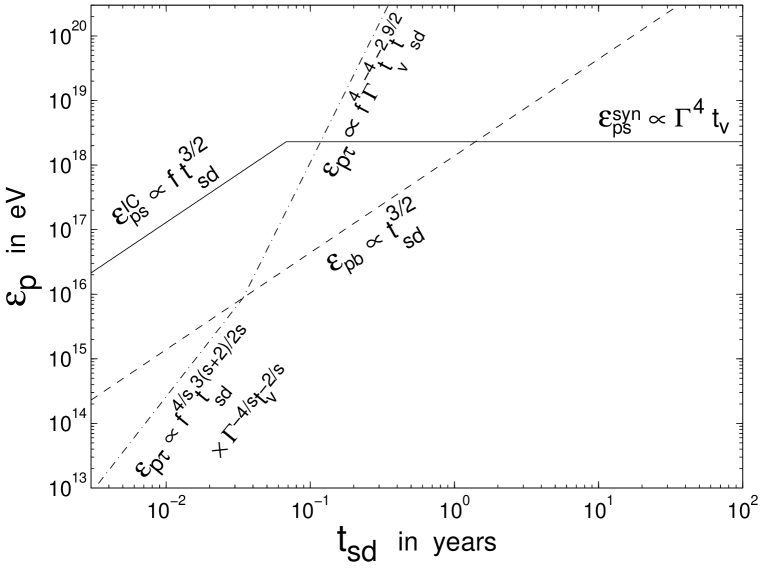
Figure 4: The proton energies that correspond to break energies in the neutrino spectrum, $\varepsilon_{\nu}\approx\varepsilon_{p}/20$, as a function of $t_{\rm sd}$. This figure is taken from Guetta & Granot 2002a

In Figure 4 we show the proton energies that correspond to the neutrino break energies $\varepsilon_{\nu s}$, $\varepsilon_{\nu b}$ and $\varepsilon_{\nu\tau}\approx\varepsilon_{p\tau}/20$, as a function of $t_{\rm sd}$. From Eq. (B2), (B8) and (B9), we conclude that $\tau_{p\gamma}\propto\Gamma^{2}t_{\rm sd}^{-3/2}$, while $\varepsilon_{ps}^{\rm syn}\propto\Gamma^{4}$ and $\varepsilon_{ps}^{\rm IC}\propto t_{\rm sd}^{3/2}$. For a fixed value of $t_{\rm sd,-1}=1$, $\Gamma_{2.5}\gtrsim 1$ implies $\tau_{p\gamma}\gtrsim 1$ and $\varepsilon_{ps}=\varepsilon_{ps}^{\rm IC}={\rm constant}\sim 10^{18}\;$eV, while $\Gamma_{2.5}\lesssim 1$ implies $\varepsilon_{ps}=\varepsilon_{ps}^{\rm syn}\propto\Gamma^{4}$. This implies increased neutrino emission reaching higher energies for larger values of $\Gamma$. Since large $\Gamma$ implies lower synchrotron frequency for the prompt GRB, this may be relevant to X-ray flashes, assuming that they are indeed GRBs with relatively large Lorentz factors and/or a large variability time, $t_{v}$ (Guetta, Spada & Waxman 2001b).

As can be seen from Figure 4, depending on the relevant parameters, there are four different orderings of these break energies: (i) $\varepsilon_{\nu\tau}<\varepsilon_{\nu b}<\varepsilon_{\nu s}$, (ii) $\varepsilon_{\nu b}<\varepsilon_{\nu\tau}<\varepsilon_{\nu s}$, (iii) $\varepsilon_{\nu b}<\varepsilon_{\nu s}<\varepsilon_{\nu\tau}$ and (iv) $\varepsilon_{\nu s}<\varepsilon_{\nu b}<\varepsilon_{\nu\tau}$. Each of these results in a different spectrum consisting of 3 or 4 power laws. Analytically these spectra are:

$${\varepsilon_{\nu}^{2}{dN_{\nu}\over d\varepsilon_{\nu}}(i)/f_{0}\;\over{(4+s)/4s+\ln(\varepsilon_{\nu s}/\varepsilon_{\nu\tau})\over\left[(4+s_{/}2s+\ln(\varepsilon_{\nu s}/\varepsilon_{\nu\tau})\right]^{2}}}=\left\{\begin{array}[]{lll}(\varepsilon_{\nu}/\varepsilon_{\nu\tau})^{s/2}&\ \ \varepsilon_{\nu}<\varepsilon_{\nu\tau}\\ 1&\ \ \varepsilon_{\nu\tau}<\varepsilon_{\nu}<\varepsilon_{\nu s}\\ (\varepsilon_{\nu}/\varepsilon_{\nu s})^{-2}&\ \ \varepsilon_{\nu}>\varepsilon_{\nu s}\end{array}\right.\ ,$$ (B10)

$${\varepsilon_{\nu}^{2}{dN_{\nu}\over d\varepsilon_{\nu}}(ii)/f_{0}\;\over{5/4+\ln(\varepsilon_{\nu s}/\varepsilon_{\nu\tau})\over\left[5/2+\ln(\varepsilon_{\nu s}/\varepsilon_{\nu\tau})\right]^{2}}}=\left\{\begin{array}[]{lll}\sqrt{\varepsilon_{\nu b}\over\varepsilon_{\nu\tau}}\left({\varepsilon_{\nu}\over\varepsilon_{\nu b}}\right)^{s\over 2}&\ \ \varepsilon_{\nu}<\varepsilon_{\nu b}\\ (\varepsilon_{\nu}/\varepsilon_{\nu\tau})^{1/2}&\ \ \varepsilon_{\nu b}<\varepsilon_{\nu}<\varepsilon_{\nu\tau}\\ 1&\ \ \varepsilon_{\nu\tau}<\varepsilon_{\nu}<\varepsilon_{\nu s}\\ (\varepsilon_{\nu}/\varepsilon_{\nu s})^{-2}&\ \ \varepsilon_{\nu}>\varepsilon_{\nu s}\end{array}\right.\ ,$$ (B11)

$${\varepsilon_{\nu}^{2}{dN_{\nu}\over d\varepsilon_{\nu}}(iii)/f_{0}\over{3\over 16}\sqrt{\varepsilon_{\nu s}\over\varepsilon_{\nu\tau}}}=\left\{\begin{array}[]{lll}\left({\varepsilon_{\nu b}\over\varepsilon_{\nu s}}\right)^{1\over 2}\left({\varepsilon_{\nu}\over\varepsilon_{\nu b}}\right)^{s\over 2}&\ \ \varepsilon_{\nu}<\varepsilon_{\nu b}\\ (\varepsilon_{\nu}/\varepsilon_{\nu s})^{1/2}&\ \ \varepsilon_{\nu b}<\varepsilon_{\nu}<\varepsilon_{\nu s}\\ (\varepsilon_{\nu}/\varepsilon_{\nu s})^{-3/2}&\ \ \varepsilon_{\nu s}<\varepsilon_{\nu}<\varepsilon_{\nu\tau}\\ \left({\varepsilon_{\nu s}\over\varepsilon_{\nu\tau}}\right)^{3\over 2}\left({\varepsilon_{\nu\tau}\over\varepsilon_{\nu}}\right)^{2}&\ \ \varepsilon_{\nu}>\varepsilon_{\nu\tau}\end{array}\right.\ ,$$ (B12)

$${\varepsilon_{\nu}^{2}{dN_{\nu}\over d\varepsilon_{\nu}}(iv)/f_{0}\over[s(4-s)/16](\varepsilon_{\nu s}/\varepsilon_{\nu b})^{s/2}\sqrt{\varepsilon_{\nu b}/\varepsilon_{\nu\tau}}}=\left\{\begin{array}[]{lll}(\varepsilon_{\nu}/\varepsilon_{\nu s})^{s/2}&\ \ \varepsilon_{\nu}<\varepsilon_{\nu s}\\ (\varepsilon_{\nu}/\varepsilon_{\nu s})^{(s-4)/2}&\ \ \varepsilon_{\nu s}<\varepsilon_{\nu}<\varepsilon_{\nu b}\\ \left({\varepsilon_{\nu b}\over\varepsilon_{\nu s}}\right)^{(s-4)/2}\left({\varepsilon_{\nu}\over\varepsilon_{\nu b}}\right)^{-3/2}&\ \ \varepsilon_{\nu b}<\varepsilon_{\nu}<\varepsilon_{\nu\tau}\\ \left({\varepsilon_{\nu b}\over\varepsilon_{\nu s}}\right)^{s-4\over 2}\left({\varepsilon_{\nu b}\over\varepsilon_{\nu\tau}}\right)^{3\over 2}\left({\varepsilon_{\nu\tau}\over\varepsilon_{\nu}}\right)^{2}&\ \ \varepsilon_{\nu}>\varepsilon_{\nu\tau}\end{array}\right.\ .$$ (B13)

For our analysis we consider two characteristic values of $t_{\rm sd}$, 0.07 yr and 0.4 yr, and refer to the models as 3 and 4, respectively. In the case of Model 3, the GRB is seen only if the shell is sufficiently clumpy while in model 4 the GRB should always be detectable.

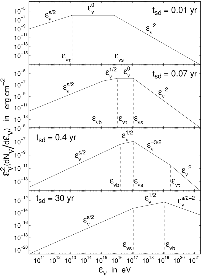
Figure 5: The muon neutrino spectrum, $\varepsilon_{\nu}^{2}(dN_{\nu}/d\varepsilon_{\nu})$, for our fiducial parameters in models 3 and 4 (interactions with PWB photons). Four choices of $t_{\rm sd}=0.01,\,0.07,\,0.4,\,30\;$yr are used, which correspond to the 4 different orderings of the break energies. This figure is taken from Guetta & Granot 2002a

The muon neutrino spectrum is shown in Figure 5 for our fiducial parameters and $t_{\rm sd}=0.01,\,0.07,\,0.4,\,30\;$yr. The spectrum of the other neutrino flavors is the same.

Appendix C Appendix: Calculations of Event Rates

A compilation of the probability that a GRB neutrino is actually detected as a muon, a tau or a shower by an underground detector is shown in Fig. 4 as a function of the neutrino energy. These are required to convert neutrino spectra from GRBs to event rates. We present in this appendix the formalism for doing this conversion.

C.1 Showers

The number of shower events in an underground detector from a neutrino flux $\Phi_{\nu_{i}}$ produced by a single GRB with duration $T$ is given by

$$N_{\rm sh} = \sum_{i,j}2\pi AT\int dE_{\nu_{i}}\frac{d\Phi_{\nu_{i}}}{dE_{\nu_{i}}}(E_{\nu_{i}})\,P_{\rm surv}(E_{\nu_{i}},\theta_{z})$$ (C1)

$$\times\int_{y^{i,j}_{\rm min}}^{y^{i,j}_{\rm max}}dy\frac{1}{\sigma^{j}(E_{\nu_{i}})}\,\frac{d\sigma^{j}}{dy}(E_{\nu_{i}},y)\,P_{\rm int}(E_{\nu_{i}},y,\theta_{z})\ ,$$

where $\theta_{z}$ is the zenith angle ($\theta_{z}=0$ is vertically downward). The sum is over neutrino (and anti-neutrino) flavors $i=e,\mu,\tau$ and interactions $j={\rm CC}$ (charged current) and NC (neutral current). $A$ is the detector’s cross sectional area with respect to the $\nu$ flux, and $d\Phi_{\nu_{i}}/dE_{\nu_{i}}$ is the differential neutrino flux that reaches the Earth. For $i=\tau$, C1 is modified to include the effects of regeneration of neutrinos propagating through the Earth, as will be discussed further on.

$P_{\rm surv}$ is the probability that a neutrino reaches the detector, i.e. is not absorbed by the Earth. It is given by

$$P_{\rm surv}\equiv\exp[-X(\theta_{z})\sigma^{\rm tot}(E_{\nu_{i}})N_{A}]\ ,$$ (C2)

where $N_{A}\simeq 6.022\times 10^{23}{\rm g}^{-1}$, and the total neutrino interaction cross section is

$$\sigma^{\rm tot}=\sigma^{\rm CC}+\sigma^{\rm NC}\ .$$ (C3)

This is somewhat conservative because it neglects the possibility of a neutrino interacting via a NC interaction and subsequently creating a shower in the detector. $X(\theta_{z})$ is the column density of material a neutrino with zenith angle $\theta_{z}$ must traverse to reach the detector. It depends on the depth of the detector and is given by

$$X(\theta_{z})=\int_{\theta_{z}}\rho(r(\theta_{z},l))\,dl\ ,$$ (C4)

the path length along direction $\theta_{z}$ weighted by the Earth’s density $\rho$ at distance $r$ from the Earth’s center. For the Earth’s density profile we adopt the piecewise continuous density function $\rho(r)$ of the Preliminary Earth Model (Dziewonski 1989).

$P_{\rm int}$ is the probability that the neutrino interacts in the detector. It is given by

$$P_{\rm int}=1-\exp\left[-\frac{L}{L^{j}(E_{\nu_{i}})}\right]\ ,$$ (C5)

where, for showers, $L$ is the linear dimension of the detector, and $L^{j}(E_{\nu_{i}})$ is the mean free path for neutrino interaction of type $j$. For realistic detectors, $L\ll L^{j}(E_{\nu_{i}})$, and so $P_{\rm int}\approx L/L^{j}(E_{\nu_{i}})$. To an excellent approximation the event rate scales linearly with detector volume $V=AL$.

The inelasticity parameter $y$ is the fraction of the initial neutrino energy carried by the hadronic shower (rather than the primary lepton). The limits of integration depend on the type of interaction and on the neutrino flavor. For NC $\nu_{e}$ interactions and all $\nu_{\mu}$ and $\nu_{\tau}$ interactions, $y_{\rm max}=1$ and $y_{\rm min}=E^{\rm thr}_{\rm sh}/E_{\nu}$, where $E^{\rm thr}_{\rm sh}$ is the threshold energy for shower detection. For CC $\nu_{e}$ interactions, the outgoing electron also showers, therefore $y_{\rm max}=1$ and $y_{\rm min}=0$.

C.2 Muons

Energetic muons are produced in $\nu_{\mu}$ CC interactions. For a muon to be detected, it must reach the detector with an energy above its threshold $E^{\rm thr}_{\mu}$. The expression of Eq.(C1) then also describes the number of muon events after the replacement

$$P_{\rm int}=1-\exp\left[-\frac{R_{\mu}(E_{\mu},\theta_{z})}{L^{\rm CC}(E_{\nu_{\mu}})}\right]\ ,$$ (C6)

where $R_{\mu}$ is the range of a muon with initial energy $E_{\mu}=(1-y)E_{\nu_{\mu}}$ and final energy $E^{\rm thr}_{\mu}$. We will assume that muons lose energy continuously according to

$$\frac{dE}{dX}=-\alpha-\beta E\ ,$$ (C7)

where $\alpha=2.0~{}{\rm MeV}{\rm cm}^{2}/{\rm g}$ and $\beta=4.2\times 10^{-6}~{}{\rm cm}^{2}/{\rm g}$ (Dutta et al. 2001). The muon range is then

$$R_{\mu}=\frac{1}{\beta}\ln\left[\frac{\alpha+\beta E_{\mu}}{\alpha+\beta E^{\rm thr}_{\mu}}\right]\ .$$ (C8)

In this case, $y_{\rm max}=1-E^{\rm thr}_{\mu}/E_{\nu}$ and $y_{\rm min}=0$.

The event rate for muons is enhanced by the possibility that muons reach the detector, even if produced in neutrino interactions kilometers from its location. Note, however, that this enhancement (i.e. $R_{\mu}$) is $\theta_{z}$-dependent: for nearly vertical down-going paths, the path length of the muon is limited by the amount of matter above the detector, not by the muon’s range. This is taken into account in the simulations. Fig.7 shows the probability of detecting a muon generated by a muon neutrino as a function of the incidence zenith angle. The figure illustrates the effect of the limited amount of matter above the detector, as well as the neutrino absorption in the Earth. Absorption is not important at $E_{\nu}=1$ TeV, and the muon range at this energy (for a muon energy threshold of 500 GeV as we adopted in the figure) is not limited by the amount of matter above the detector. As a consequence the probability at 1 TeV is weakly dependent on zenith angle. Absorption in the Earth starts to be important for upgoing neutrinos of energy above $\sim 100$ TeV - 1 PeV, and restricts the neutrino observation to the horizontal and downward directions at extremely high energy (EeV range) as can be seen in the figure. The large muon range at PeV and EeV energies, much larger than the depth at which the detector is located (1.8 km vertical depth), reduces considerably the detection probability of downgoing neutrinos.

The largest background to a GRB signal consists of muons from atmospheric neutrinos. However, for GRB observations, the time and angular windows are very small and this background can be easily controlled, as we will illustrate. Following (Dermer & Atoyan 2003), the number of background events is approximately given by

$$N_{\rm{bg}}\simeq A\int d\Omega\int dt\int^{\infty}_{E_{\rm{min}}}dE_{\nu}\frac{dN_{\nu}}{dE_{\nu}}P_{\nu\rightarrow\mu}(E_{\nu})$$ (C9)

where $\Omega$ and $t$ are the solid angle and time considered, respectively, and $P_{\nu\rightarrow\mu}(E_{\nu})$ is the probability of a muon neutrino generating a muon in the detector volume. IceCube is designed to have angular resolution smaller than 1 degree at the relevant energies. We consider a 1 degree cone for the solid angle calculation. Considering a long burst of duration $\sim 100$ seconds, and using the following approximate atmospheric neutrino spectrum

$$\frac{dN_{\nu}}{dE_{\nu}}=\left\{\begin{array}[]{lll}5\times 10^{-18}E_{\nu}^{-4}\,\rm{GeV}\,\rm{cm}^{-2}\,\rm{s}^{-1}\,\rm{sr}^{-1}&\ \ E_{\nu}>10^{5}\rm{GeV}\\ 1.6\times 10^{-16}E_{\nu}^{-3.7}\,\rm{GeV}\,\rm{cm}^{-2}\,\rm{s}^{-1}\,\rm{sr}^{-1}&\ \ \ E_{\nu}<10^{5}\rm{GeV}\\ \end{array}\right.\ ,$$ (C10)

we find that for a natural threshold (minimum energy) of $\sim 100\,$GeV, we expect $\sim.003$ background events per burst. More practically, an energy threshold in the range of 1-10 TeV could be imposed which would reduce this background by an addition factor of 50 to 2500, respectively. For a naive illustration, consider one years of observation, with 1000 bursts, each of duration of 10 seconds and a 1 TeV energy threshold imposed. For such a example, less than 0.01 total background events are predicted.

C.3 Taus

Taus are produced only by CC $\nu_{\tau}$ interactions. This process differs significantly from the muon case because tau neutrinos are regenerated by the production and subsequent tau decay through $\nu_{\tau}\to\tau\to\nu_{\tau}$ (Halzen & Saltzberg 1998). As a result, for tau neutrinos, CC and NC interactions in the Earth do not deplete the $\nu_{\tau}$ flux, they only reduce the neutrino energy down to a value where, eventually, the Earth becomes transparent. We implement this important effect using a dedicated simulation that determines $\overline{E}_{\nu_{\tau}}(E_{\nu_{\tau}},\theta_{z})$, the average energy of the $\nu_{\tau}$ when reaching the detector. It depends on the initial energy $E_{\nu_{\tau}}$ and zenith angle $\theta_{z}$. The tau event rate is then given by

$$N_{\tau} = 2\pi AT\int dE_{\nu_{\tau}}\frac{d\Phi_{\nu_{\tau}}}{dE_{\nu_{\tau}}}(E_{\nu_{\tau}})\int_{y_{\rm min}}^{y_{\rm max}}dy\frac{1}{\sigma^{\rm CC}(\overline{E}_{\nu_{\tau}})}\frac{d\sigma^{\rm CC}}{dy}(\overline{E}_{\nu_{\tau}},y)$$ (C11)

$$\times P_{\rm int}\Theta((1-y)\overline{E}_{\nu_{\tau}}-E^{\rm thr}_{\tau})\ ,$$

$P_{\rm int}$ depends on the geometry of the neutrino tau induced event. For events consisting on a minimum-ionizing track going through the detector it is given by:

$$P_{\rm int}=\left[1-\exp\left(-\frac{R_{\tau}((1-y)\overline{E}_{\nu_{\tau}})}{L^{\rm CC}(\overline{E}_{\nu_{\tau}})}\right)\right]$$ (C12)

where $R_{\tau}((1-y)\overline{E}_{\nu_{\tau}})$ is the range of the produced tau evaluated at the energy of the tau after regeneration. $R_{\tau}$ is given by Eq.(C8) with $\beta=3.6\times 10^{-7}~{}{\rm cm}^{-2}/{\rm g}$ (Dutta et al. 2001). The last factor takes into account the requirement that the tau track be long enough to be identified in the detector. We require $E^{\rm thr}_{\tau}\simeq 2.5\times 10^{6}~{}\;$GeV so that the tau decay length is larger than the 125  m string spacing in IceCube. It is not clear with what efficiency through-going tau events can be separated from low energy muons.

Those tau events that include one shower (lollipop events) or two showers (double bang events) inside the detector volume will be identifiable. For these cases we use $P_{\rm int}$ obtained by a dedicated simulation that determines the probabilities for double bang and lollipop geometries shown in Fig.(6). The rate of downgoing lollipop events in a km³ neutrino telescope is expected to be of the order of the rate of down-going shower events, probably slightly smaller. Double bang events will be mostly observed for neutrino energies in a limited range between roughly 10 and 100 PeV.

Finally, those events in which the tau decays into muons that reach the detector are counted as muon events. $P_{\rm int}$ is given by Eq.(C12) where we use as range the sum of the range of the tau evaluated at the regeneration energy and the range of the muon at the energy that carries in the decay of the tau.

As with muons, at very high energies taus can travel several kilometers before decaying or suffering significant energy loss. The enhancement to tau event rates from this effect is $\theta_{z}$-dependent as discussed above for muons.

Figure 1: The distribution of (a) redshifts, (b) Lorentz factors, (c) fluences and (d) zenith angles (for muon events: dotted line corresponds to model 1, solid line to model 2) for long duration GRBs. In (a), the decrease at large redshift is due to sampling bias. The Lorentz factors in (b) were calculated as described by Eqs. A17 and  A18. Frame (d) demonstrates the advantages of long muon range and poor absorption near the horizon for muon track detection.

Figure 2: The distribution of the estimated number of muon events from individual (a) long duration GRBs (the dotted line corresponds to model 1 and the solid line to model 2) and (b) X-ray flash candidates (dotted line corresponds to model 3 and the solid line to model 4). Note that the majority of events result from a relatively small number of GRBs.

Figure 3: The muon neutrino spectrum, $\varepsilon_{\nu}^{2}(dN_{\nu}/d\varepsilon_{\nu})$, for our fiducial parameters in models 1 and 2 (interactions with GRB photons). The solid line is for a typical GRB with $\Gamma=300$ and $t_{v}=10$ ms, while the dashed line is for a X-ray flash candidate with $\Gamma=1440$ (calculated from Eq. A18) and $t_{v}=50$ ms.

Figure 6: The probabilities of a neutrino generating various types of events when traveling through the effective area of a neutrino telescope. Curves are shown for various choices of zenith angle, which reflects enhancements due to long muon range and the effect of absorption in the Earth.

Figure 7: The probability of a muon neutrino generating a detectable muon as a function of zenith angle. The curves show the probabilities for three representative neutrino energies: $10^{12}$ eV, $10^{15}$ eV and $10^{18}$ eV.

References

- (1) Alvarez-Muñiz, J., Halzen, F. & Hooper D. W., 2000, PRD, 62, 093015.
- (2) Andres, E. et al., 2001, Nature 410, 441.
- (3) Aslanides, E., et al. for the ANTARES Collaboration, 1999, astro-ph/9907432.
- (4) Barouch, G & Hardtke, R., talk given at the International Cosmic Ray Conference, 2001.
- (5) Dermer, C. & Atoyan, A., 2003, submitted to PRL, astro-ph/0301030.
- (6) Dutta, S. I., Reno, M. H., Sarcevic, I. & Seckel, D., 2001, PRD, 63, 094020.
- (7) Dziewonski, A. “Earth Structure, Global,” in The Encyclopedia of Solid Earth Geophysics, edited by D. E. James (Van Nostrand Reinhold, New York, 1989), p.331.
- (8) Eichler, D., et al., 1989, Nature, 340, 126
- (9) Fenimore, E. E. & Ramirez-Ruiz, E., 2000, in press on ApJ, astro-ph/0004176.
- (10) Fishman, G. J. & Meegan, C. A., 1995, ARA&A 33, 415.
- (11) Freedman, D., Waxman, E., 2001, ApJ, 547.
- (12) Fryer, C., & Woosley, S.E., 1998, ApJ, 502, L9.
- (13) Fryer, C., Woosley, S.E., & Hartmann, D.H., 1999, ApJ, 526, 152.
- (14) Gaisser, T. K., Halzen, F., Stanev, T., 1995, Phys. Rep., 173.
- (15) Guetta D. & Granot J., 2003, Phys. Rev. Lett. 90, 201103. astro-ph/0212045.
- (16) Guetta D. & Granot J., 2003, MNRAS 340, 115, astro-ph/0208156.
- (17) Guetta D. & Granot J., 2003, ApJ 585, 885, astro-ph/0209578.
- (18) Guetta D., Spada M., & Waxman E., 2001a, ApJ 559, 101.
- (19) Guetta D., Spada M., & Waxman E., 2001b, ApJ 557, 339.
- (20) Halzen, F. & Hooper, D. W., 1999, ApJ 527, L93.
- (21) Halzen, F. & Hooper, D. W., 2002, Rept. Prog. Phys. 65, 1025.
- (22) Halzen, F. & Saltzberg, D., 1998, PRL 81, 4305.
- (23) Heise, J., Zand, J. J., Kippen, M. & Woods, P., Gamma-Ray Bursts in the Afterglow Era, Proceedings of the International workshop held in Rome, CNR headquarters, 17-20 October, 2000. Edited by Enrico Costa, Filippo Frontera, and Jens Hjorth. Berlin Heidelberg: Springer, 2001, p. 16. astro-ph/0111246.
- (24) Inoue, S., Guetta, D., & Pacini, F., 2003, ApJ, 583, 379.
- (25) Kippen, R. M. et al., 2002, astro-ph/0203114.
- (26) Kobayashi, S., Ryde, F., & MacFadyen, A., 2002 ApJ, 577, 302.
- (27) Königl, A., & Granot, J. 2002, ApJ, 574, 134.
- (28) Lazzati, D. et al., 2001, ApJ 556, 471.
- (29) Learned, J. G. & Mannheim, K., 2000, Ann. Rev. Nucl. Part. Sci. 50, 679.
- (30) Lloyd-Ronning, N., & Ramirez-Ruiz, E., 2002, ApJ, 576, 101.
- (31) McBreen, S., Quilligan, F., McBreen, B., Hanlon L. & Watson D., astro-ph/0206294.
- (32) Narayan, R., Paczński, B., & Piran, T. 1992, ApJ, 395, L83.
- (33) Norris, J. P., Marani, G. F. & Bonnell, J. T.,2000, ApJ, 534, 248.
- (34) Paciesas, W. S., Preece, R. D. Briggs, M. S. & Mallozzi, R. S., Gamma-Ray Bursts in the Afterglow Era, Proceedings of the International workshop held in Rome, CNR headquarters, 17-20 October, 2000. Edited by Enrico Costa, Filippo Frontera, and Jens Hjorth. Berlin Heidelberg: Springer, 2001, p. 13. astro-ph/0109053.
- (35) Paczński, B. 1998, ApJ, 494, 45.
- (36) Piro, L., et al., 2000, Science 290, 955.
- (37) Razzaque, S., Mészáros, P. & Waxman, E., 2002, submitted to PRL, astro-ph/0212536.
- (38) Rees, M. J., & Mészáros, P., 1994, ApJ, 430, L93
- (39) Reichart, D. E. et al., 2001, ApJ, 552, 57.
- (40) Reichart D. E. & Lamb, D. Q., Gamma-Ray Bursts in the Afterglow Era, Proceedings of the International workshop held in Rome, CNR headquarters, 17-20 October, 2000. Edited by Enrico Costa, Filippo Frontera, and Jens Hjorth. Berlin Heidelberg: Springer, 2001, p. 233. astro-ph/0103254.
- (41) Sari, R., & Piran, T. 1997, ApJ, 485, 270
- (42) Vietri M., 1995, ApJ, 453, 883
- (43) Vietri, M., 1998a, ApJ, 507, 40.
- (44) Vietri, M., 1998b, PRL, 80, 3690.
- (45) Vietri, M. & Stella, L. 1998, ApJ, 507, L45.
- (46) Vietri M., et al., 2001, ApJ 550, L43.
- (47) Vietri, M., De Marco, D. & Guetta, D., 2003, ApJ in press, astro-ph/0302144
- (48) Waxman, E., 1995, PRL, 75, 386.
- (49) Waxman, E., & Bahcall, J., 1997, PRL, 78, 2292.
- (50) Waxman, E., & Bahcall, J., 2000, ApJ, 541, 707.
- (51) Gamma-Ray Bursts in the Afterglow Era, Proceedings of the International workshop held in Rome, CNR headquarters, 17-20 October, 2000. Edited by Enrico Costa, Filippo Frontera, and Jens Hjorth. Berlin Heidelberg: Springer, 2001, p. 263.
- (52) Woosley, S.E. 1993, ApJ, 405, 273
- (53) Zhang, B., & Meszaros, P., 2002, ApJ, 581, 1236.