Fermi and Swift Gamma-Ray Burst Afterglow Population Studies

Abstract

The new and extreme population of GRBs detected by Fermi-LAT shows several new features in high energy gamma-rays that are providing interesting and unexpected clues into GRB prompt and afterglow emission mechanisms. Over the last 6 years, it has been Swift that has provided the robust dataset of UV/optical and X-ray afterglow observations that opened many windows into components of GRB emission structure. The relationship between the LAT detected GRBs and the well studied, fainter, less energetic GRBs detected by Swift-BAT is only beginning to be explored by multi-wavelength studies. We explore the large sample of GRBs detected by BAT only, BAT and Fermi-GBM, and GBM and LAT, focusing on these samples separately in order to search for statistically significant differences between the populations, using only those GRBs with measured redshifts in order to physically characterize these objects. We disentangle which differences are instrumental selection effects versus intrinsic properties, in order to better understand the nature of the special characteristics of the LAT bursts.

1. Introduction

The field of gamma-ray bursts (GRBs) is undergoing dramatic changes for a second time within the past decade, as a new observational window has opened with the launch and success of NASA’s Fermi gamma-ray space telescope. While both NASA’s Swift gamma-ray burst explorer mission (Gehrels et al. 2004) and Fermi are operating simultaneously, we have the ability to potentially detect hundreds of gamma-ray bursts per year ($\sim 1/3$ of which are triggered by Swift). This allows prompt observations in the $15-150$ keV hard X-ray band with the Burst Alert Telescope (BAT, Barthelmy et al. 2005) and rapid follow-up in the $0.3-10$ keV soft X-ray band with the X-Ray Telescope (XRT, Burrows et al. 2005) and the UV/optical band by the Ultraviolet Optical Telescope (UVOT, Roming et al. 2005) on-board Swift. There is $\sim 40\%$ overlap between BAT triggers and triggers from Fermi’s Gamma-ray Burst Monitor (GBM, Meegan et al. 2009) allowing for coverage from 10 keV to 30 MeV, and a special subset detected up to 10s of GeV with Fermi’s Large Area Telescope (LAT, Atwood et al. 2009). This wide space-based spectral window is broadened further by ground based optical, NIR, and radio follow-up observations.

In the last 2 years, the addition of the 30 MeV to 100 GeV window from Fermi-LAT has led to another theoretical crisis, as we attempt to understand the origin and relationship between these new observational components and the ones traditionally observed from GRBs in the keV-MeV band. Just as Swift challenged our theoretical models by demonstrating that GRBs have complex behavior in the first few hours after the trigger (Nousek et al. 2006), Fermi-LAT is regularly observing a new set of high energy components in a small very energetic subset of bursts (Abdo et al. 2009a, b, c, 2010; Ackermann et al. 2010). The relationship between the $>100$ MeV emission and the well studied keV-MeV components remains unclear (Corsi et al. 2010a, b; Kumar & Barniol Duran 2010; Razzaque et al. 2010; Zhang & Pe’er 2009; Ghisellini et al. 2010; Pe’er et al. 2010; Piran & Nakar 2010; Toma et al. 2010; Wang et al. 2010).

The complicated Fermi-LAT prompt emission spectra do not show simply the extension of the lower-energy Band function (Band et al. 1993), but rather the joint GBM-LAT spectral fits can also show the presence of an additional hard power-law that can be detected both above and below the Band function (Abdo et al. 2009a; Ackermann et al. 2010) in some cases. There were earlier indications of this additional spectral component in the EGRET detected GRB 941017 (González et al. 2003). However, the rarity of EGRET GRB detections left it unclear whether this was a common high energy feature, or if special circumstances in that GRB were responsible. This component is too shallow to be due to Synchrotron self-Compton (SSC) as had been predicted extensively pre-Fermi (Zhang & Mészáros 2001; Guetta & Granot 2003; Galli & Guetta 2008; Racusin et al. 2008; Band et al. 2009). The spectral behavior of the LAT bursts appears to rule out the theory that the soft $\gamma$-rays are caused by a SSC or another Inverse Compton (IC) component (Ando et al. 2008; Piran et al. 2009).

Fermi-LAT’s $>100$ MeV temporal behavior is different from the lower-energy counterparts observed from thousands of GRBs. The LAT emission often begins a few seconds later than the lower-energy prompt emission, and sometimes lasts substantially longer (up to thousands of seconds; Abdo et al. 2009a, c; Ackermann et al. 2010). This so-called “GeV extended emission” and the extra spectral power-law component may be the same component, but the statistics in the extended emission are limited and detailed spectral fits are often not possible.

Several groups (Ghisellini et al. 2010; Kumar & Barniol Duran 2010; de Pasquale et al. 2010) suggest that the high-energy extended emission is caused by the same forward shock mechanism (with special caveats for environmental density and magnetic field strength) responsible for the well studied broadband afterglows that have been observed for hundreds of other GRBs. Alternatively, Zhang et al. (2011); Maxham et al. (2011) suggest that the $>100$ MeV emission during the prompt emission phase is of internal origin, and the later extended emission is of external origin. We can learn more about the mysterious new LAT components by studying the GRBs from a broadband perspective, for which the early broadband afterglow (specifically X-ray and optical) behavior is well studied. However, currently there is only one case of simultaneous X-ray/optical/GeV emission in the minutes after the GRB - the short hard GRB 090510 which was simultaneously triggered upon the Swift-BAT and the Fermi-GBM and LAT (de Pasquale et al. 2010).

Despite the lack of simultaneous LAT and lower energy observations in long bursts, we can still learn about the special nature of the LAT bursts by studying their lower energy late-time afterglow observations. In this paper, we utilize the large database of Swift afterglow observations of BAT discovered bursts, and compare them to the simultaneous BAT/GBM triggers, and the Swift follow-up of the LAT/GBM detected bursts, in order to learn about the properties of the different populations of GRBs.

This paper is organized as follows: in Section 2 we discuss the sample selection and data analysis, in Section 3 we discuss the results and correlations apparent in the different samples, in Section 4 we discuss the physical implications of our analysis, and in Section 5 we conclude.

2. Sample Selection and Analysis

In order to study the population differences between the BAT-triggered sample, the GBM-triggered sample, and the LAT detected sample, we use all GRBs from these samples with measured redshifts and well constrained XRT and UVOT light curves (at least 4 light curve bins and enough counts to construct and fit an X-ray spectrum).

As of December 2009, the Swift XRT and UVOT instruments have observed afterglows of 439 bursts discovered by BAT, as well as 81 bursts discovered by other missions. We now have enough detailed observations of X-ray and UV/optical afterglows from Swift to study them as a statistical sample, and to attempt to separate observational biases from physical differences in GRB populations. In this study, we included afterglow observations of all GRBs discovered by Swift-BAT between December 2004 and December 2009 (sample hereafter referred to as BAT), with measured redshifts in the literature (e.g. Fynbo et al. 2009) and well-constrained light curves and spectra.

Unfortunately, the positional errors provided by GBM are too large (several degrees) to facilitate Swift follow-up. Therefore, the only afterglow observations we have of GBM triggered bursts, are those that simultaneously triggered the Swift-BAT and meet all of the same criteria as the BAT sample (sample hereafter referred to as GBM). We treat the GBM bursts separately from the BAT sample, and do not include them in both samples. The GBM bursts have a much wider measured spectral range during the prompt emission than the BAT bursts, and are therefore more likely to provide an accurate measurement of $E_{peak}$ and the Band function parameters. From an instrumental perspective, BAT has a much better sensitivity than GBM. Therefore, the GBM bursts are biased towards higher fluence.

We also include the LAT detected GBM triggered GRBs that have been localized by XRT and UVOT in follow-up observations (sample hereafter referred to as LAT). The LAT position errors for those GRBs for which follow-up was initiated were $\sim 3-10$ arcminutes radius. Those GRBs with initial position errors that were significantly larger than the XRT field of view (FoV) have not been followed-up by Swift. The LAT sample includes the one BAT/GBM/LAT simultaneous trigger (GRB 090510), and the remaining LAT detected GRBs that BAT did not observe (i.e. were outside the BAT FoV at trigger). There has been follow-up of 10 out of 24 LAT detected GRBs (as of March 2011) with position errors small enough to initiate Target of Opportunity (ToO) observations. However, (with the exception of the joint BAT/GBM/LAT trigger) these follow-up observations began at a minimum of 12 hours after the trigger, and in some cases, did not begin until 1-2 days post-trigger. Despite this impediment, 8 of 10 LAT GRBs were detected by XRT, and 7 of 10 by UVOT (5 in u-band, see Section 2.2).

The breakdown of GRBs in each of the XRT and UVOT datasets for the BAT, GBM, and LAT samples are given in Table 1. Individual bursts are included in only one of the BAT, GBM, and LAT samples, depending on their detection by one, two, or all three instruments. In the following Sections, we describe the data analysis of the follow-up X-ray and UV/optical observations, as well as the methods and sources for obtaining $\gamma$-ray prompt emission spectral fits and fluences.

Table 1Sample Statistics

Sample	XRT	UVOT
BAT	147	49
GBM	19	11
LAT	8	5

Note. — The number of GRBs in each sample that meet our selection criteria. For a GRB to be included in the UVOT sample, observations in the u-band are needed for normalization.

2.1. X-ray

The X-ray light curves and spectral fits were obtained from the XRT team repository (Evans et al. 2007, 2009). We fit and characterized all of the light curves using the methods of Racusin et al. (2009). Each count rate light curve was fit with the best fitting model of either a power law, broken power law, double broken power law, or triple broken power law, after time periods of significant flaring were manually removed.

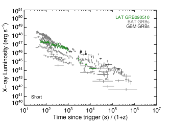
Figure 1.— The X-ray (0.3-10 keV) afterglow rest-frame luminosity light curves for all of the long (top panel) and short (bottom panel) GRBs in our samples. The BAT, GBM, and LAT GRBs are indicated by the different colors. Note the clustering of the LAT light curves compared to the BAT and GBM samples in the top panel.

We convert the count-rate light curves to flux light curves based on a single counts-to-flux conversion factor obtained from the Photon Counting (PC) mode spectral fit. In order to physically characterize the afterglows, taking advantage of the redshift information, we convert flux to luminosity and apply a k-correction using the following formalism from Berger et al. (2003a):

$$L_{x}(t)=4\pi D_{L}^{2}F_{x}(t)(1+z)^{\alpha_{x}-\beta_{x}-1}$$ (1)

where $L_{x}(t)$ is the $0.3-10~{}\textrm{keV}$ luminosity at time $t$ seconds after the trigger; $F_{x}$ is the $0.3-10~{}\textrm{keV}$ flux at time $t$; $D_{L}$ is the luminosity distance assuming cosmological parameters: $H_{0}=71~{}\textrm{km}~{}\textrm{s}^{-1}~{}\textrm{Mpc}^{-1}$, $\Omega_{m}=0.27$, and $\Omega_{\Lambda}=0.73$; $\alpha_{x}$ is the X-ray power-law temporal decay at time $t$; and $\beta_{x}$ is the spectral energy index at time $t$. The X-ray luminosity light curves in rest frame time for both the long and short bursts, for all three of our samples, are shown in Figure 1.

The X-ray spectra were also taken from the XRT team repository. Evans et al. (2009) describes how the spectra are extracted and fit to absorbed power-laws, with two absorption components (Galactic and intrinsic at the GRB redshift). The spectral power-law index ($\Gamma$) is converted to the energy index via $\beta=\Gamma-1$, where $F_{x}=t^{-\alpha_{x}}\nu^{-\beta_{x}}$.

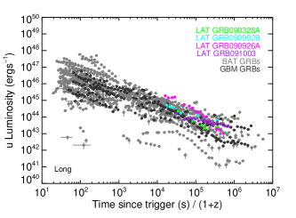
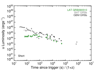
Figure 2.— The u-band normalized afterglow rest-frame luminosity light curves for all of the long (top panel) and short (bottom panel) GRBs in our samples. The BAT, GBM, and LAT GRBs are indicated by the different colors.

2.2. UV/Optical

The UV/Optical light curves were obtained from the second UVOT GRB catalog (Roming et al., 2011, in-preparation) and combined such that the 5 arcsec extraction region light curves were used at count rates $>0.5~{}\textrm{counts~{}s}^{-1}$, and 3 arcsec extraction region at lower count rates. We combined the UVOT 7 filter light curves (where available and detected) using the methods of Oates et al. (2009) in order to obtain the highest signal-to-noise light curves. This involves first normalizing the individual filter light curves for each GRB to a single band, then combining and rebinning. We chose to normalize all of the UVOT light curves in this study to the UVOT u-band in order to optimize the number of LAT GRB afterglow light curves that could be used in this comparison, because that was the most commonly used filter for the LAT burst follow-up. Note that although 7 of the Swift followed-up LAT bursts were detected by UVOT (compared to 8 by XRT), we could only obtain detailed u-band light curves for five. The others (GRB 090323 and GRB 100414A) were only detected in the white filter, which cannot be normalized to the u-band without knowing the shape of the optical spectrum, and also cannot be easily used to extract luminosity information because of the flat wide transmission curve of this filter. Note that GRB 080916C was detected by XRT, but not UVOT, which is consistent with the redshift (z=4.35, Greiner et al. 2009).

We convert the UVOT count rate light curves from observed count rate to flux via the average GRB u-band conversion factor provided by Poole et al. (2008). We also correct for Galactic extinction, and correct for host galaxy extinction by fitting broadband (XRT and UVOT) Spectral Energy Distributions (SEDs) choosing the best fit dust model (MW, LMC, SMC) for each burst using the methods of Schady et al. (2010). The conversion from flux to luminosity is similar to that of the X-ray luminosities given in Equation 1. Using the optical spectral index from the SEDs, we calculate the u-band k-corrected luminosity as:

$$L_{o}(t)=4\pi D_{L}^{2}F_{o}(t)(1+z)^{\alpha_{o}-\beta_{o}-1}.$$ (2)

where $F_{o}=t^{-\alpha_{o}}\nu^{-\beta_{o}}$, and $F_{o}$ is the u-band flux at time $t$.

We fit the count rate light curves in a similar manner to that of the X-ray light curves, except that we allow an additional constant contribution to the power-law fits to account for the flattening occasionally observed in UVOT light curves. This flattening can be due to either host galaxy contribution or nearby source contamination. By simply allowing the fit to include this extra constant, we can subtract it off and extrapolate the power-law fit to the time of interest.

The u-band rest frame luminosity light curves for the short and long bursts for each of our BAT, GBM, and LAT samples are shown in Figure 2. The light curve shapes have not been altered to adjust for the extra constant.

2.3. $\gamma$-ray

Due to the different $\gamma$-ray instruments used to detect the GRBs in our samples, observational biases cause much of the differences between these samples. Likely, the only differences between the GBM and BAT samples are related to the larger and harder energy range of the GBM, and the superior sensitivity of the BAT. However, Swift has had 6.5 years to collect a sample of GRBs with a wide range of spectral properties and brightness. This is reflected in the ranges of the X-ray and UV/Optical afterglow light curves. The LAT sample on the other hand, although a subset of the GBM sample, has inherent differences. $50\%$ of the GBM bursts occur within the LAT field-of-view, but only a small fraction $<5\%$ are detected. For the LAT to detect a GRB, the prompt emission must have a very high fluence. The factors that may contribute to the high fluence in the $30~{}\textrm{MeV}-100~{}\textrm{GeV}$ bandpass include the spectrum peaking at relatively high energies, the spectrum having a very shallow $\beta_{Band}$ index, and the presence of an additional hard power law component (as has been detected in several LAT bursts).

In Section 3.5, we discuss burst energetics based upon observations and limits from afterglow light curves. The prompt emission spectral fits used in these calculations were obtained from several sources. The BAT spectral fits and fluences come from the second BAT GRB catalog (Sakamoto et al. 2011). The GBM spectral fits come from either individual burst papers in the literature, or GCN circulars. Fluences were recalculated from these fits in several different bandpasses for the calculation of $E_{\gamma,iso}$ and prompt emission fluence ratios.

3. Results

Using our compiled luminosity rest frame light curves and SEDs, we explored various parameters for differences and similarities between the BAT, GBM, and LAT burst populations. The goal was to determine whether the LAT detected GRBs are fundamentally different from the normal BAT and GBM samples, or whether they are simply the extreme cases.

Unfortunately, except in the case of the short GRB 090510, we do not have any early afterglow observations of the LAT bursts, therefore we limit measurements to times for which all data sets are available. One day after the trigger in the rest frame is within the BAT, GBM, and LAT observations, though we also compare some properties at 11 hours (a standard observed frame time used in other papers including de Pasquale et al. 2006 and Gehrels et al. 2008). For the cases of Swift bursts, when no data are available at this time, we extrapolate from the earlier power-law decay index.

3.1. Temporal and Spectral Indices

Using the light curve fits described in Sections 2.1 and 2.2, we collect the power-law decay indices at a rest frame time of 1 day. Typically this is the decay index in the normal forward shock phase (post-plateau, pre-jet break) in the X-ray light curves (Zhang et al. 2006; Nousek et al. 2006; Racusin et al. 2009). In the cases where the light curves end prior to 1 day (rest frame), we take the final decay index. The UV/optical light curve behavior observed by UVOT has a different early morphology, often with an initial rise followed by a shallow decay and occasionally later steepening (Oates et al. 2009). Oates et al. (2009) observed that the distribution of $\alpha_{o}$ after 500 s (post-trigger) is similar to $\alpha_{x}$ during the plateau phase, suggesting that the optical afterglows are also affected by energy injection at early times, or their temporal profile deviates due to a break (e.g. cooling break) between the two bands.

Similarly, we also extract the X-ray and optical spectral indices ($\beta_{x}$ and $\beta_{o}$), and plot them against the temporal indices in Figure 3. There is significant scatter in both the temporal and spectral properties, and no significant correlation.

We note that $\alpha_{o}$ is systematically lower than $\alpha_{x}$ at 1 day in the rest frame, though many of the UVOT light curves were extrapolated from earlier observations to their expected later behavior assuming no breaks.

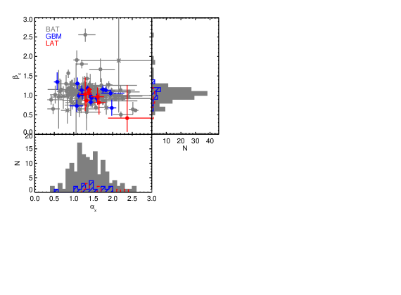
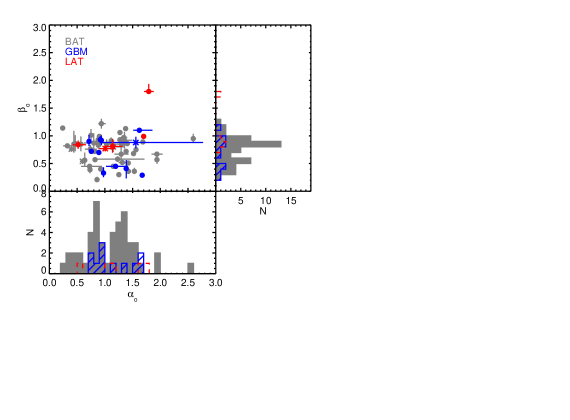
Figure 3.— The temporal and spectral decay indices at 1 day in the rest frame interpolated from the X-ray (top panel) and optical (bottom panel) afterglow fits. The scatter plots and histograms show that there are no noticeable differences between the BAT, GBM, and LAT populations.

There is little correlation in either the X-ray or optical temporal and spectral indices, as expected (given the variety of possible closure relations, Racusin et al. 2009). From these distributions, one can see that there are no noticeable differences between the BAT, GBM, and LAT populations. Kolmogorov-Smirnov (K-S) tests confirm that there are no statistically significant differences between the populations in these measurements (Table 2).

3.2. Redshift

Redshift is another physical quantity that we can evaluate for each of our GRB populations, with separation into short and long populations. Jakobsson et al. (2006) (later updated by Fynbo et al. 2009) showed that Swift GRBs are on average at a higher redshift ($\sim 2.2$ versus $\sim 1.5$) than pre-Swift populations, likely due to the superior sensitivity of the Swift-BAT and softer energy range than previous instruments. It would therefore follow that the GBM and LAT redshift distributions may be different. Of course these are instrumental selection effects, and as we will discuss in Section 3.4, the LAT bursts tend to have brighter optical afterglows than BAT bursts, therefore are more likely to have redshift measurements of their optical transients.

With our limited statistics, there are no significant differences (measured with K-S tests, Table 2) between the redshift distributions of the BAT, GBM, and LAT populations as illustrated in Figure 4. However, these are not independent samples, as the GBM bursts were all also detected by BAT and localized by XRT/UVOT, and these are only the brightest best localized LAT bursts. Despite these caveats, there is no evidence of any differences in redshift distributions.

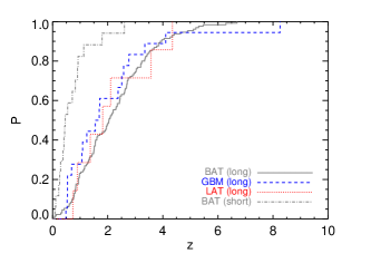
Figure 4.— Cumulative distribution functions of the long and short burst redshift distributions of the BAT, GBM, and LAT GRB populations in our sample. Note that no distributions are plotted for the short GBM and short LAT bursts, because only one GRB is present in each of those samples.

3.3. Environment

Using the parameters from the SED fits, we can constrain measurements of the X-ray absorption ($N_{H}$) or approximate gas content and the optical extinction ($A_{V}$) or approximate dust content, in order to learn about the GRB environments. After we remove the Galactic absorption and extinction contributions, these quantities probe the environment around the GRB progenitor and along the line of sight. Figure 5 demonstrates these extinction and absorption measurements separated into the BAT, GBM, and LAT samples. While a K-S test (Table 2) does not show any significant differences between the populations in either $N_{H}$ or $A_{V}$, the small number of LAT bursts for which we could make these measurements tend toward lower values of $A_{V}$ with moderate values of $N_{H}$.

The crude gas-to-dust ratios ($N_{H}/A_{V}$, Figure 6) for each of the different best fit dust models (MW, LMC, SMC) show two features that might distinguish the LAT bursts: the LAT bursts are all best fit by the SMC extinction law, and they tend towards high values of the gas-to-dust ratio. Since many of the $A_{V}$ measurements of the LAT bursts are upper limits, this makes the corresponding $N_{H}/A_{V}$ ratios lower limits, which would only further distinguish the LAT bursts. Due to the low $A_{V}$ values (even $A_{V}=0$) of the LAT bursts, they can be fit by any of the the three extinction laws equally well (Schady et al. 2010). The gas-to-dust ratio intrinsically depends on several factors including the original pre-GRB environmental ratio of gas-to-dust, and the amount of dust destruction and photoionization during the GRB event in close proximity to the bursts. Properties of the GRB itself such as amount and spectrum of the energy output influence the alteration of the environment. Therefore, understanding differences in the final gas-to-dust ratio is clouded by these factors which are difficult to disentangle between properties of the environment and the GRB itself. This measurement is also model dependent, and can be biased by assumptions about the spectral model. Regardless, the LAT bursts appear to have little to no dust along the line-of-sight compared to the GBM and BAT bursts.

At this time, there are insufficient statistics on gas and dust content of the LAT bursts to draw any strong conclusions from this sample. Further study with more objects and broader band data are needed to distinguish any strong environmental differences between these populations.

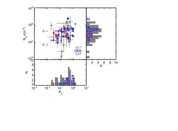
Figure 5.— Intrinsic X-ray absorption ($N_{H}$) plotted against visual dust extinction ($A_{V}$) measured from the SED fits described in Section 2.2.

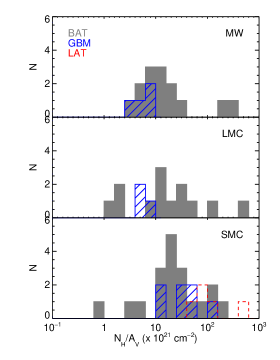
Figure 6.— $N_{H}/A_{V}$ or gas-to-dust ratio for all of the GRBs in the BAT, GBM, and LAT samples for the three best fit dust extinctions models (MW, LMC, SMC) for each GRB.

3.4. Afterglow Luminosity

The luminosity light curves in Figures 1 and 2 reveal several interesting observational and possibly intrinsic differences between the BAT, GBM, and LAT populations. The GBM and to a higher extent LAT X-ray afterglows are clustered much more than the BAT afterglows. From an instrumental perspective, BAT is more sensitive to detecting faint GRBs than GBM, therefore having a wider and fainter distribution of X-ray afterglows (that correlates with prompt fluence, Gehrels et al. 2008) is reasonable. However, due to the correlation between $\gamma$-ray fluence and X-ray flux, with the LAT GRBs having comparatively extreme fluences (Swenson et al. 2010; Cenko et al. 2011; McBreen et al. 2010; Ghisellini et al. 2010), we would have expected the LAT GRBs to be at the bright end of the X-ray afterglow distribution. This distribution is present in all permutations of these light curves (count rate, flux, flux density, luminosity), so it is not an effect of one of our count rate to flux, flux density, or luminosity correction factors.

This unexpected distribution is shown more clearly in the histograms of Figure 7, demonstrating a cross-section of the luminosity at 11 hours and 1 day in the rest frame of each GRB.

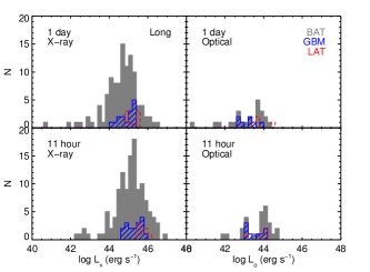
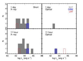
Figure 7.— Histograms of X-ray (0.3-10 keV, left column) and optical (u band, right column) instantaneous luminosity at times of 11 hours (bottom row) and 1 day (top row) in the rest frame of each GRB, with the long bursts (top panel) and short bursts (bottom panel) separated. Notice that the LAT long burst population luminosities are larger on average than that of the other samples, but are not at the very bright end of the distribution.

3.5. Energetics

With this large sample of X-ray and optical afterglows, redshifts, and simple assumptions about the environment and physical parameters, we can estimate the total isotropic equivalent $\gamma$-ray energy output in a systematic way over the same energy range for all of the GRBs in our samples. Despite the fact that we do not have accurate measurements of $E_{peak}$ for most of the BAT bursts, we can estimate both $E_{peak}$ (using the power law index correlation from Sakamoto et al. 2009), and either estimate the Band function or cutoff power law parameters, use typical values, or use measurements from other instruments with larger energy coverage (e.g. Konus-Wind, Fermi-GBM, Suzaku-WAM) especially if they have constrained $E_{peak}$. Using the assumed spectrum for each GRB and the measured redshift, we integrate over a common rest frame energy range (Amati et al. 2002) of 10 keV to 10 MeV, as:

$$E_{\gamma,iso}=\frac{4\pi D_{L}^{2}}{(1+z)}\int_{10~{}keV/(1+z)}^{10~{}MeV/(1+z)}E~{}F(E)~{}dE.$$ (3)

The functional forms and assumptions are described in more detail in the appendix of Racusin et al. (2009). Using this method, we infer a reasonable value of $E_{\gamma,iso}$ for each GRB in a systematic way.

Ghisellini et al. (2010) and Swenson et al. (2010) established that LAT GRBs include some of the most energetic GRBs ever detected. On average, the LAT GRBs have isotropic equivalent $\gamma$-ray energy outputs ($E_{\gamma,iso}$) that are 1-2 orders of magnitude larger than that of the Swift bursts (Figure 8). Given the well known correlations between $E_{peak}$ and $E_{\gamma,iso}$ (Amati et al. 2002; Amati 2006), and the hardness of LAT GRB spectra required for them to be detected by LAT at all, their large $E_{\gamma,iso}$’s are not surprising.

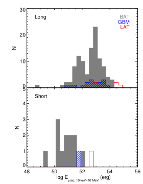
Figure 8.— Distribution of $E_{\gamma,iso}$ for both long (top panel) and short (bottom panel) bursts in the BAT, GBM, and LAT samples. The GBM and BAT distributions are statistically similar. However, the LAT GRBs are on average more energetic than the other samples and extend above $10^{55}$ ergs.

This suggests to us that the LAT is preferentially detecting extremely energetic GRBs compared to previous GRB experiments. The sensitivity, large field of view, and large energy range of the LAT make it especially sensitive to hard bursts. While the physical origin of the Amati relation is not well understood, the energetic LAT bursts seem to qualitatively follow the same relationship.

Applying our characterizations of the optical and X-ray light curves and SEDs to the energetics, we can infer jet half-opening angles and collimation-corrected $\gamma$-ray energy outputs ($E_{\gamma}$), or limits when all observations were either pre- or post-jet break. Again, the methods used in these calculations and jet break determination are described in detail in Racusin et al. (2009).

Using the XRT and UVOT data alone, most of the LAT GRB afterglow light curves (exceptions discussed below) are best characterized by single power laws, with relatively flat slopes ($\alpha_{o,x}\lesssim 1.8$), with the exception of the poorly sampled GRB 100414A which may have had a break in the large gap between observations, and the short GRB 090510 which shows an early break to a steep decay - a behavior suggestive of a “naked” short hard burst (Kumar & Panaitescu 2000) that indicates the turnoff of the prompt emission in a low density environment with either an afterglow too faint to detect or no afterglow at all. However, de Pasquale et al. (2010) discussed the possibility that the break in the optical and X-ray light curves of GRB 090510 at $\sim 2000$ seconds is an early jet break, rather than a naked afterglow (i.e. steep fall off is either high latitude emission or post-jet break). The following calculations use the jet break assumption, but we recommend caution when examining the energetics of this GRB.

The LAT optical light curves, where sampled well, show shallow behavior or contamination at late times by the host galaxy or nearby sources. This is consistent with the idea that most of the LAT afterglow observations are pre-jet break (with the exceptions noted above). Several recent papers (McBreen et al. 2010; Cenko et al. 2011; Swenson et al. 2010) suggest that when using other broadband observations (including deep late optical/NIR observations), some of these bursts do hint at jet breaks, but the Swift data alone are insufficient to constrain jet breaks. We will discuss the differences in jet breaks and energetics between this paper and those of McBreen et al. (2010); Cenko et al. (2011); Swenson et al. (2010) further in Section 4.

If we assume all of the LAT GRBs are pre-jet break (except for GRB 100414A, which may be post jet break, and GRB 090510, which may include a jet break), and we determine the presence of jet breaks in the X-ray afterglows of the BAT and GBM samples using the criteria from Racusin et al. (2009), we can evaluate the jet opening angles and collimation-corrected energetics as a function of these populations, as shown in Figure 9.

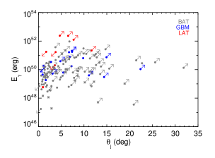
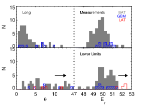
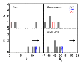
Figure 9.— $E_{\gamma}$ as a function of $\theta_{j}$ (top panel) for the BAT, GBM, and LAT samples, for both long and short bursts, including, pre- and post-jet break. Arrows indicate lower or upper limits on jet break times that translate into limits on $\theta_{j}$ and $E_{\gamma}$. Histograms of $\theta_{j}$ and $E_{\gamma}$ for the long bursts (middle panel) and short bursts (bottom panel) including both measurements (upper plots) and upper limits (lower plots) as indicated in the top panel scatter plot. Note that the LAT burst are at the upper end of the $E_{\gamma}$ distribution in comparison to the BAT and GBM samples, and are only lower limits.

For those GRBs with only lower limits on the jet break times, we use the time of last detection to determine the lower limit on $\theta_{j}$, and therefore also $E_{\gamma}$. As demonstrated in Racusin et al. (2009), there are several different characteristic times for which one can place limits on jet breaks, and the large error bars on late-time light curve data points can mask jet breaks (see also Curran et al. 2008). However, for Figure 9, we simply use the time of last detection.

Table 2K-S Test Probabilities

Parameter	BAT-GBM	BAT-LAT	GBM-LAT
Long Bursts
$\alpha_{x}$	0.78	0.14	0.54
$\alpha_{o}$	0.93	0.44	0.63
$\beta_{x}$	0.95	0.59	0.87
$\beta_{o}$	0.63	0.27	0.16
$z$	0.55	0.95	0.76
$A_{V}$	0.33	$9.0\times 10^{-2}$	$6.8\times 10^{-2}$
$N_{H}$	0.31	0.64	0.76
$N_{H}/A_{V}(\times 10^{21})$	0.19	$5.3\times 10^{-3}$	$3.0\times 10^{-2}$
$L_{x,11hr}$	0.27	$2.2\times 10^{-3}$	$5.3\times 10^{-2}$
$L_{x,1day}$	0.36	$1.2\times 10^{-2}$	0.18
$L_{o,11hr}$	0.38	0.29	$4.8\times 10^{-2}$
$L_{o,1day}$	0.44	0.21	$7.8\times 10^{-2}$
$E_{\gamma,iso}$	0.39	$1.3\times 10^{-3}$	$1.4\times 10^{-2}$
$\theta_{j}$	0.15	–	–
$E_{\gamma}$	$4.7\times 10^{-2}$	–	–

Note. — Probabilities of the two distributions being drawn from the same parent population from K-S tests. Small values indicate significant differences between the samples. Dashes indicate that there were not enough ($\geq 2$) bursts that fit relevant criteria to perform a K-S test. Only long burst statistics are included here, because there were not enough short hard bursts to perform K-S tests on the GBM and LAT populations.

4. Discussion

We have showed that there are observational differences between the BAT, GBM, and LAT samples throughout the previous sections. However, the difficulty lies in separating out the instrumental selection effects from the physical differences between GRBs that produce appreciable $>100~{}\textrm{MeV}$ emission, and those that do not.

The median and standard deviation of the distributions of the many observational parameters discussed in the previous and following sections are presented for each sample in Table 3.

In the following section, we will explore physical explanations for the observable parameter distributions including a calculation of the radiative efficiency, and speculate on the origin of the afterglow luminosity clustering. We also will compare and contrast the other recent studies of the broadband observations of the LAT bursts.

Table 3Parameter Population Characterizations

Parameter	BAT long	GBM long	LAT long	BAT short	GBM short	LAT short
$\alpha_{x}$	$1.46~{}(0.56,~{}130)$	$1.43~{}(0.35,~{}18)$	$1.58~{}(0.38,~{}7)$	$1.50~{}(0.82,~{}12)$	$1.22$	$2.19$
$\alpha_{o}$	$1.21~{}(0.76,~{}46)$	$1.11~{}(0.35,~{}10)$	$1.29~{}(0.59,~{}4)$	$0.72~{}(0.39,~{}3)$	$1.56$	$1.01$
$\beta_{x}$	$1.08~{}(0.37,~{}130)$	$1.02~{}(0.18,~{}18)$	$0.90~{}(0.25,~{}7)$	$0.96~{}(0.34,~{}12)$	$1.14$	$0.79$
$\beta_{o}$	$0.74~{}(0.24,~{}48)$	$0.75~{}(0.29,~{}13)$	$1.11~{}(0.47,~{}4)$	$0.70~{}(0.14,~{}3)$	$0.88$	$0.77$
$z$	$2.21~{}(1.35,~{}130)$	$2.06~{}(1.88,~{}18)$	$2.12~{}(1.36,~{}7)$	$0.71~{}(0.65,~{}17)$	$1.37$	$0.90$
$A_{V}~{}(\textrm{mag})$	$0.32~{}(0.28,~{}44)$	$0.48~{}(0.35,~{}12)$	$0.11~{}(0.13,~{}3)$	$0.32~{}(0.20,~{}2)$	$0.40$	–
$log~{}N_{H}~{}(\textrm{cm}^{-2})$	$20.87~{}(2.95,~{}130)$	$21.22~{}(2.53,~{}18)$	$19.52~{}(3.27,~{}7)$	$21.17~{}(0.45,~{}12)$	$21.26$	$20.95$
$log~{}L_{x,11~{}hr}~{}(\textrm{erg~{}s}^{-1})$	$45.06~{}(0.83,~{}120)$	$45.28~{}(0.39,~{}17)$	$45.72~{}(0.24,~{}7)$	$43.26~{}(2.14,~{}12)$	$45.00$	$42.82$
$log~{}L_{x,1~{}day}~{}(\textrm{erg~{}s}^{-1})$	$44.62~{}(0.89,~{}106)$	$44.87~{}(0.40,~{}15)$	$45.19~{}(0.30,~{}7)$	$42.72~{}(2.47,~{}11)$	$44.59$	$42.08$
$log~{}L_{o,11~{}hr}~{}(\textrm{erg~{}s}^{-1})$	$43.72~{}(0.71,~{}27)$	$43.57~{}(0.47,~{}8)$	$44.33~{}(0.57,~{}4)$	$43.12$	$43.27$	$43.08$
$log~{}L_{o,1~{}day}~{}(\textrm{erg~{}s}^{-1})$	$43.11~{}(0.98,~{}23)$	$43.19~{}(0.42,~{}7)$	$43.86~{}(0.41,~{}4)$	$42.98$	–	–
$log~{}E_{\gamma,iso}~{}(\textrm{erg})$	$52.56~{}(0.87,~{}105)$	$52.66~{}(0.88,~{}17)$	$54.01~{}(0.75,~{}7)$	$50.81~{}(0.74,~{}12)$	$51.83$	$52.59$
$\theta_{j}~{}(\textrm{deg})$	$3.53~{}(3.63,~{}55)$	$4.73~{}(3.20,~{}9)$	–	$4.46~{}(4.93,~{}4)$	–	$0.99$
$\theta_{j,lim}~{}(\textrm{deg})$	$9.19~{}(6.34,~{}46)$	$10.68~{}(6.36,~{}8)$	$7.65~{}(2.95,~{}4)$	$12.28~{}(4.13,~{}5)$	$11.74$	–
$log~{}E_{\gamma}~{}(\textrm{erg})$	$49.73~{}(0.71,~{}55)$	$50.30~{}(0.64,~{}9)$	–	$48.31~{}(1.03,~{}4)$	–	$48.77$
$log~{}E_{\gamma,lim}~{}(\textrm{erg})$	$50.20~{}(0.80,~{}46)$	$50.36~{}(0.74,~{}8)$	$52.04~{}(0.49,~{}4)$	$48.99~{}(0.79,~{}5)$	$50.15$	–
$log~{}E_{k}~{}(\textrm{erg})$	$53.41~{}(0.85,~{}47)$	$53.52~{}(0.43,~{}12)$	$53.69~{}(0.44,~{}6)$	$52.40~{}(1.09,~{}3)$	$53.05$	–
$\eta~{}(\%)$	$17.58~{}(23.34,~{}47)$	$19.94~{}(19.15,~{}12)$	$64.80~{}(22.53,~{}6)$	$6.06~{}(4.63,~{}3)$	$5.69$	–

Note. — Mean of the distributions of each parameter for the BAT, GBM, and LAT samples, separated into long and short bursts. Numbers in parentheses indicate standard deviation and the number of objects in each parameter distribution. There is only one object in each of the GBM and LAT short burst samples.

4.1. Radiative Efficiency

Our first attempt to explore the underlying physics is by calculating the radiative efficiency of the GRBs at turning their kinetic energy into radiation during the prompt emission. We follow the formulation of Zhang et al. (2007), which derives the kinetic energy ($E_{k}$) from the X-ray afterglow observations, and by comparing the $\gamma$-ray prompt emission output, we can estimate a radiative efficiency:

$$\eta=\frac{E_{\gamma,iso}}{E_{\gamma,iso}+E_{k}}$$ (4)

where $E_{k}$ depends on the synchrotron spectral regime (Sari et al. 1998, $\nu>\nu_{c}$ or $\nu<\nu_{c}$) as:

$$E_{k,52,\nu>\nu_{c}}=\left(\frac{\nu F_{\nu}}{5.2\times 10^{-14}~{}\textrm{ergs}~{}\textrm{s}^{-1}~{}\textrm{cm}^{-2}}\right)^{4/(p+2)}$$

$$\times~{}D_{28}^{8/(p+2)}(1+z)^{-1}~{}t_{d}^{(3p-2)/(p+2)}$$

$$~{}(1+Y)^{4/(p+2)}~{}f_{p}^{-4/(p+2)}~{}\epsilon_{B,-2}^{(2-p)/(p+2)}$$

$$\times~{}\epsilon_{e,-1}^{4(1-p)/(p+2)}~{}\nu_{18}^{2(p-2)/(p+2)}$$ (5)

$$E_{k,52,\nu<\nu_{c}}=\left(\frac{\nu F_{\nu}}{6.5\times 10^{-13}~{}\textrm{ergs}~{}\textrm{s}^{-1}~{}\textrm{cm}^{-2}}\right)^{4/(p+3)}$$

$$\times~{}D_{28}^{8/(p+3)}(1+z)^{-1}~{}t_{d}^{3(p-1)/(p+3)}$$

$$\times~{}f_{p}^{-4/(p+3)}~{}\epsilon_{B,-2}^{-(p+1)/(p+3)}$$

$$\times~{}\epsilon_{e,-1}^{4(1-p)/(p+3)}~{}n^{-2/(p+3)}~{}\nu_{18}^{2(p-3)/(p+2)}.$$ (6)

All subscripts indicate the convention $X_{n}=X/10^{n}$ in cgs units. $D_{28}$ is the luminosity distance in units of $10^{28}$ cm, $t_{d}$ is the time of interest in units of days, $p$ is the electron spectral index derived from the spectral index $\beta_{x}$ where:

$$p=\begin{cases}2\beta_{x}+1&\nu<\nu_{c}\\ 2\beta_{x}&\nu>\nu_{c}\\ \end{cases}$$ (7)

and

$$f_{p}=6.73\left(\frac{p-2}{p-1}\right)^{(p-1)}(3.3\times 10^{-6})^{(p-2.3)/2}.$$ (8)

We make several simplifying assumptions including using a single typical value for $\epsilon_{e}=0.1$, $\epsilon_{B}=0.01$, and $n=1~{}\textrm{cm}^{-3}$ as well as ignoring inverse Compton emission ($Y=1$). Unlike Zhang et al. (2007), we do not determine the kinetic energy ($E_{k}$) at the deceleration time or the break time, because we do not have the temporal context of the shallow decay phase (the earlier or later canonical phases) in many bursts, including the LAT bursts. Instead, we calculated $\eta$ at observed times of 11 hours and 1 day, but only if there was evidence from the light curve morphology and decay slopes of those measurements being during the normal decay (forward shock) phase (Zhang et al. 2006; Racusin et al. 2009). The efficiency did not change significantly between these two times, but more GRB X-ray afterglows were in the normal decay phase at 11 hours than at 1 day. Therefore, the 11 hour results are plotted in Figure 10. We determined whether a particular X-ray afterglow was above or below the cooling frequency ($\nu_{c}$) using the closure relations and assuming the simplest cases ($p>2$, ISM or Wind environments, slow cooling, no energy injection), similarly to Zhang et al. (2007).

Figure 10 demonstrates the relationship between the kinetic energy and the $\gamma$-ray prompt emission with the range of radiative efficiencies indicated. Only 69 GRBs are included in this plot. The rest of our sample were excluded either due to not having sufficient information to measure $E_{\gamma,iso}$, not satisfying the relevant closure relations, lack of a clear normal forward shock decay, or lack of emission at time of interest (in this case 11 hours in the observed frame). Of the 69 GRBs, 51 are from the BAT sample, 12 from the GBM sample, and 6 from the LAT sample.

Our measured efficiencies for the BAT sample cover a similar range and roughly agree with their statement from Zhang et al. (2007) that given the above assumptions, most ($\sim 57\%$) of BAT bursts have $\eta<10\%$. This statement is not true for the GBM and LAT samples. In fact, only $25\%$ of the GBM bursts have $\eta<10\%$, and none of the LAT bursts have such low radiative efficiencies. This suggests that GBM and LAT detected GRBs are on average more efficient at converting kinetic energy into prompt radiation, which perhaps explains why they are substantially brighter (higher fluence) than the BAT bursts with similar afterglow luminosities. The LAT bursts are at the high end of the $E_{\gamma,iso}$-$E_{k}$ distributions with $\eta>40\%$ for all LAT bursts, and $\eta>80\%$ for three of the LAT bursts. These extreme efficiencies may be unphysical and due to a our assumptions: an internal shock mechanism as is described in the fireball model (Rees & Mészáros 1998; Mészáros 2002), a single value of $\epsilon_{e}$ and $\epsilon_{B}$, no appreciable Compton component, and a single universal surrounding medium density.

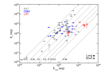
Figure 10.— Kinetic energy ($E_{k}$) derived from the X-ray afterglow observations at 11 hours as a function of the prompt emission isotropic equivalent $\gamma$-ray energy output ($E_{\gamma,iso}$). The dashed lines indicated different values of the radiative efficiency ($\eta$). The LAT bursts tend to have high $E_{\gamma,iso}$ but average $E_{k}$, and therefore higher values of $\eta$ than the BAT or GBM samples.

We acknowledge that these differences in the distribution of $\eta$ are degenerate with differences in $\epsilon_{e}$, $\epsilon_{B}$, and the presence of some inverse Compton component. We also caution that our estimations of $E_{\gamma,iso}$ for the LAT bursts do not include the extra spectral power law observed in several of the LAT bursts. However, that would make $\eta$ even larger, which perhaps suggests that it is the internal shock model framework that is not valid.

4.2. Bulk Lorentz Factor

The bulk Lorentz factor ($\Gamma$) is a fundamental quantity needed to describe the GRB fireball and therefore interesting to compare for different populations of bursts. Unfortunately, it is also a difficult quantity to accurately measure and there are several methods for placing lower or upper limits on this quantity depending on multiple assumptions.

The most common technique applied to the Fermi-LAT detected bursts (Abdo et al. 2009c; Ackermann et al. 2010; Abdo et al. 2009a) was originally derived by Lithwick & Sari (2001), using the highest energy observed photon to place a lower limit on the $\gamma$-ray pair production attenuation, setting a lower limit on $\Gamma$. This method assumes that the GeV and seed sub-MeV photons are emitted from the same co-spatial region and are produced by internal shocks. It can produce extreme values of $\Gamma\gtrsim 1000$ for the LAT bursts. Zhao et al. (2011) and Zou et al. (2011) suggest modifications for this calculation using a two-zone model that assumes that the sub-MeV and GeV photons are produced at very different radii from the central engine. This modification lowers $\Gamma$ to approximately a few hundred. Hascoët et al. (2011, in-preparation) also demonstrate that when carefully calculating the pair production attenuation taking into account the jet geometry and dynamics, $\Gamma$ is reduced by a factor of $\sim 2.5$.

When no high energy (GeV) observations are available, the most common method to limit $\Gamma$ is to derive it from the deceleration time of the forward shock which corresponds to the peak time of the optical (Sari & Piran 1999; Molinari et al. 2007; Oates et al. 2009; Liang et al. 2010) or X-ray (Liang et al. 2010) afterglow light curves. Often one can only set upper limits on the deceleration time because the peak must have occurred prior to the start of the observations, corresponding to lower limits on $\Gamma$, or be buried under other components.

There are additional alternative methods to determine $\Gamma$ including putting upper limits on the forward shock contribution to the keV-MeV prompt emission by looking for deep minima or dips down to the instrumental threshold between peaks in the prompt emission light curves (Zou & Piran 2010). The typical values of these upper limits on $\Gamma$ are several hundred. Pe’er et al. (2007) describe another method that estimate $\Gamma$ from the thermal component modeling in the prompt emission spectrum using photosphere modeling. Zhang et al. (2003) describe yet another method to estimate $\Gamma$ using early optical data to constrain the forward and reverse shock components. The latter two methods are worth further study, but the application of them to the data presented here is beyond the scope of this paper.

We apply the deceleration time of the optical light curves technique to our sample for those GRBs with UVOT light curves and measurements of $E_{k}$ (derived in Section 4.1). Unfortunately, due to the lack of early observations of the LAT bursts, we cannot apply this method to that sample. However, we collect estimates of $\Gamma$ using the pair-production attenuation technique from the literature, using the typical one-zone model from Abdo et al. (2009a, c); Ackermann et al. (2010, 2011)), as well as the two-zone estimates from Zou et al. (2011), and compare these limits in Figure 11.

The different methods yield a wide range of $\Gamma$ for each burst ranging from a few 10s to more than 1000. However, many of these results are upper or lower limits. The assumptions put into each measurement and method about the geometry and nature of the outflow have a strong influence on the results. If we believe that the sub-MeV and GeV photons are generated in the same co-spatial region, and ignore the two-zone model estimates, the lower limits on $\Gamma$ of the LAT bursts are nearly a factor of 2 higher than the BAT and GBM bursts. Unfortunately, we do not have high energy observations of many of the BAT bursts, and we do not have early optical observations of the LAT bursts, therefore one should compare measurements of $\Gamma$ for these different samples with caution.

A more careful detailed study of bulk Lorentz factor estimates for the bursts in this sample would perhaps provide more insight into concrete differences between the samples. This would require detailed analysis of all of the prompt emission light curves and spectra of the bursts in our sample, and this is beyond the scope of this study.

It is also interesting to note that the high $\Gamma$ limits on the LAT bursts are reminiscent of a structured jet model, such as the two-component jet model where there is a narrow bright faster core surrounded by a slow wider jet, with the narrow jet on-axis to the observer (Berger et al. 2003b; Huang et al. 2004; Racusin et al. 2008). Liu & Wang (2011) explore this model using the broadband data on the LAT GRB 090902B and find an acceptable fit. Additional study of the other LAT GRBs in the context of this model would be needed to draw any stronger conclusions about the sample as a whole.

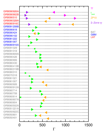
Figure 11.— Estimates of the bulk Lorentz factors ($\Gamma$) using the four methods described in Section 4.2 with different colors indicating method. The four methods are referred to as $\gamma\gamma$ - the pair production attenuation method from Lithwick & Sari (2001); $t_{peak}$ - the forward shock estimation from the optical peak described by Sari & Piran (1999); Molinari et al. (2007); ZP10 - the limit on forward shock contribution to the sub-MeV prompt emission described in Zou & Piran (2010); 2-Zone $\gamma\gamma$ - the pair production attenuation method assuming the sub-MeV and GeV photon come from different sources as described in Zou et al. (2011). A right pointing triangle indicates a lower limit, a left pointing triangle an upper limit, and an asterisk indicates a measurement. These measurements or limits are either from our own calculations (only $t_{peak}$ method) or from the literature. The bursts for which we could make measurements are shown and separated into each of the BAT, GBM, and LAT samples.

4.3. Afterglow Luminosity Clustering

As mentioned in Section 3.4, the X-ray and UV/optical luminosity distributions of the LAT bursts are narrower than the GBM and BAT samples. There are several possible causes or simply related dependencies, namely, the fact that a larger fraction of the LAT bursts are in the synchrotron spectral regime $\nu>\nu_{c}$ ($83\%$) compared to the BAT and GBM bursts ($50-60\%$), and that the LAT bursts have a narrow distribution (in log space) of $E_{\gamma,iso}$. The high radiative efficiencies of the LAT bursts may be either another cause of the narrow luminosity distribution or a consequence.

The region of luminosity parameter space fainter than the LAT bursts could be limited by the lower detection limits of the LAT instrument, and the ability to accurately localize only the brightest of the LAT burst for Swift follow-up. Nearly half of the LAT detections had position errors $>0.5$ degrees radius, which was simply not practical to initiate follow-up observations beginning many hours or days after the triggers. In the future, if Swift happens to simultaneously trigger on one of these fainter long bursts with a marginal LAT detection and a fainter afterglow, then we will know whether the luminosity clustering is only limited on the bright end.

4.4. Luminosity Function

In addition to the simple redshift distribution comparison, we explore the luminosity functions of the different populations of GRBs. We use the methods of both Virgili et al. (2009) and Wanderman & Piran (2010), which apply different statistical methods to constrain the luminosity function shapes for the three samples. Simply due to instrumental selection effects, the BAT, GBM, and LAT samples probe different regions of the luminosity function. GRBs bright enough to trigger GBM, will be brighter on average than BAT only bursts, because GBM is less sensitive than BAT. The LAT GRBs have the highest fluence of the GBM bursts, and given the similar redshift distributions (Section 3.2), are therefore also the most luminous.

The Virgili et al. (2009, 2011) method compares Monte Carlo simulations of the full parameter space drawn from the full Swift sample to the specific sample of interest, in order to be less biased by instrumental selection effects. Whereas, the Wanderman & Piran (2010) method does a more tradition fit to the observed data assuming a single value for the various instrument sensitivity levels. Both methods find consistent results for the BAT sample, fitting to a broken power law with slopes of $0.2$ and $1.4$ for the less and more luminous ends, respectively, and a break luminosity of $10^{52.5}~{}\textrm{erg}~{}\textrm{s}^{-1}$. Within the substantial error bars, the GBM sample resembles the BAT luminosity function, but does not probe as faint. The limited LAT sample is even smaller, and mostly brightward of the break luminosity. Therefore, it is best fit by a single power law with slope of 0.3, shallower than the post-break slope of the BAT and GBM functions. This shallow slope may suggest some differences in the parent population of the LAT burst, or may simply be due to the complicated selection effects of both LAT burst detection and the subset with accurate enough positions to initiate follow-up. Perhaps with a larger LAT sample, this could be studied more thoroughly. The bright end of the luminosity function of the BAT sample may not be well enough probed to accurately constrain the shape of the luminosity function, and therefore the LAT bursts are essential tools to study the most luminous GRBs ever detected.

4.5. Comparisons to Detailed Broadband Modeling

Several other recent papers (Cenko et al. 2011; McBreen et al. 2010; Swenson et al. 2010) did detailed broadband modeling of individual LAT bursts. Swenson et al. (2010) also made comparisons of the LAT bursts to prompt emission and afterglow parameters including prompt fluence and afterglow luminosities, and found that the LAT bursts had higher X-ray count rates than $80\%$ of BAT bursts at 70 ks. Note that our sample is different (only those with redshifts) and likely biased towards optically brighter bursts, and we measure luminosities rather than count rates. However we agree (also with McBreen et al. 2010) that the optical afterglows of the long LAT bursts are in the top half of the brightness distribution.

We also agree with the aforementioned works, that the LAT bursts are some of the most energetic GRBs ever observed by any instrument, and even with collimation corrections or limits on the collimation, they remain extreme events. We do not clearly detect any jet breaks in the LAT bursts using the XRT and UVOT data alone, except for perhaps the short burst GRB 090510, as discussed in Section 3.5. Both McBreen et al. (2010) and Cenko et al. (2011) claim jet breaks for some of the LAT bursts, given their ground based deep NIR and radio observations, but most are not well constrained. Clearly, more late time deep broadband observations (both space and ground-based) are needed for the LAT bursts in the future to constrain their total energetics.

5. Conclusions

We have systematically characterized the X-ray and UV/optical temporal and spectral afterglow and prompt emission characteristics, energetics, and other properties of the GRBs detected only by Swift-BAT, those detected by both Fermi-GBM and Swift-BAT, and those detected by both Fermi-GBM and LAT in order to understand the observational and intrinsic differences between the burst populations. There are no significant differences between the BAT, GBM, and LAT populations in terms of X-ray and optical temporal power law decays at common rest frame late times, or spectral power law indices, redshifts, or luminosities. However, the distributions of luminosities are much more narrow for the LAT and GBM samples compared to the BAT sample. The LAT long burst sample is also more luminous on average than the BAT sample, but within the same distribution. There are significant differences between the populations in terms of isotropic equivalent $\gamma$-ray energies ($E_{\gamma,iso}$), prompt emission hardness, and radiative efficiency.

While in many ways, the late-time ($\sim 1$ day) properties of the LAT bursts are similar to their lower energy counterparts observed by BAT, some mechanism fundamentally makes their prompt $\gamma$-ray production more efficient, or conversely suppresses their afterglows. As we collect more statistics on this exciting sub-population of GRBs detected by LAT, we can study luminous and energetic extremes. Studying the afterglows of the LAT burst, especially at early times, will also help us to understand the additional components (extra spectral power-law and extended $>100$ MeV emission) observed in many of these LAT bursts. Additional future simultaneous triggers between BAT and LAT will provide more information on the early broadband behavior of LAT bursts.

References

- Abdo et al. (2009a) Abdo, A. A., et al. 2009a, ApJ, 706, L138
- Abdo et al. (2009b) —. 2009b, ApJ, 707, 580
- Abdo et al. (2009c) —. 2009c, Science, 323, 1688
- Abdo et al. (2010) —. 2010, ApJ, 712, 558
- Ackermann et al. (2010) Ackermann, M., et al. 2010, ApJ, 716, 1178
- Ackermann et al. (2011) —. 2011, ApJ, 729, 114
- Amati (2006) Amati, L. 2006, MNRAS, 372, 233
- Amati et al. (2002) Amati, L., et al. 2002, A&A, 390, 81
- Ando et al. (2008) Ando, S., Nakar, E., & Sari, R. 2008, ApJ, 689, 1150
- Atwood et al. (2009) Atwood, W. B., et al. 2009, ApJ, 697, 1071
- Band et al. (1993) Band, D., et al. 1993, ApJ, 413, 281
- Band et al. (2009) Band, D. L., et al. 2009, ApJ, 701, 1673
- Barthelmy et al. (2005) Barthelmy, S. D., et al. 2005, Space Science Reviews, 120, 143
- Berger et al. (2003a) Berger, E., Kulkarni, S. R., & Frail, D. A. 2003a, ApJ, 590, 379
- Berger et al. (2003b) Berger, E., et al. 2003b, Nature, 426, 154
- Burrows et al. (2005) Burrows, D. N., et al. 2005, Space Science Reviews, 120, 165
- Cenko et al. (2011) Cenko, S. B., et al. 2011, ApJ, 732, 29
- Corsi et al. (2010a) Corsi, A., Guetta, D., & Piro, L. 2010a, A&A, 524, A92+
- Corsi et al. (2010b) —. 2010b, ApJ, 720, 1008
- Curran et al. (2008) Curran, P. A., van der Horst, A. J., & Wijers, R. A. M. J. 2008, MNRAS, 386, 859
- de Pasquale et al. (2006) de Pasquale, M., et al. 2006, A&A, 455, 813
- de Pasquale et al. (2010) —. 2010, ApJ, 709, L146
- Evans et al. (2007) Evans, P. A., et al. 2007, A&A, 469, 379
- Evans et al. (2009) —. 2009, MNRAS, 397, 1177
- Fynbo et al. (2009) Fynbo, J. P. U., et al. 2009, ApJS, 185, 526
- Galli & Guetta (2008) Galli, A., & Guetta, D. 2008, A&A, 480, 5
- Gehrels et al. (2004) Gehrels, N., et al. 2004, ApJ, 611, 1005
- Gehrels et al. (2008) —. 2008, ApJ, 689, 1161
- Ghisellini et al. (2010) Ghisellini, G., Ghirlanda, G., Nava, L., & Celotti, A. 2010, MNRAS, 403, 926
- González et al. (2003) González, M. M., Dingus, B. L., Kaneko, Y., Preece, R. D., Dermer, C. D., & Briggs, M. S. 2003, Nature, 424, 749
- Greiner et al. (2009) Greiner, J., et al. 2009, A&A, 498, 89
- Guetta & Granot (2003) Guetta, D., & Granot, J. 2003, ApJ, 585, 885
- Huang et al. (2004) Huang, Y. F., Wu, X. F., Dai, Z. G., Ma, H. T., & Lu, T. 2004, ApJ, 605, 300
- Jakobsson et al. (2006) Jakobsson, P., et al. 2006, A&A, 447, 897
- Kumar & Barniol Duran (2010) Kumar, P., & Barniol Duran, R. 2010, MNRAS, 1243
- Kumar & Panaitescu (2000) Kumar, P., & Panaitescu, A. 2000, ApJ, 541, L51
- Liang et al. (2010) Liang, E., Yi, S., Zhang, J., Lü, H., Zhang, B., & Zhang, B. 2010, ApJ, 725, 2209
- Lithwick & Sari (2001) Lithwick, Y., & Sari, R. 2001, ApJ, 555, 540
- Liu & Wang (2011) Liu, R.-Y., & Wang, X.-Y. 2011, ApJ, 730, 1
- Maxham et al. (2011) Maxham, A., Zhang, B.-B., & Zhang, B. 2011, MNRAS, 691
- McBreen et al. (2010) McBreen, S., Krühler, T., Rau, A., Greiner, J., Kann, D. A., Savaglio, S., Afonso, P., Clemens, C., Filgas, R., Klose, S., Küpcü Yoldaş, A., Olivares E., F., Rossi, A., Szokoly, G. P., Updike, A., & Yoldaş, A. 2010, A&A, 516, A71+
- Meegan et al. (2009) Meegan, C., et al. 2009, ApJ, 702, 791
- Mészáros (2002) Mészáros, P. 2002, ARA&A, 40, 137
- Molinari et al. (2007) Molinari, E., et al. 2007, A&A, 469, L13
- Nousek et al. (2006) Nousek, J. A., et al. 2006, ApJ, 642, 389
- Oates et al. (2009) Oates, S. R., et al. 2009, MNRAS, 395, 490
- Pe’er et al. (2007) Pe’er, A., Ryde, F., Wijers, R. A. M. J., Mészáros, P., & Rees, M. J. 2007, ApJ, 664, L1
- Pe’er et al. (2010) Pe’er, A., et al. 2010, ApJ, submitted, arXiv:1007.2228
- Piran & Nakar (2010) Piran, T., & Nakar, E. 2010, ApJ, 718, L63
- Piran et al. (2009) Piran, T., Sari, R., & Zou, Y. 2009, MNRAS, 393, 1107
- Poole et al. (2008) Poole, T. S., et al. 2008, MNRAS, 383, 627
- Racusin et al. (2008) Racusin, J. L., et al. 2008, Nature, 455, 183
- Racusin et al. (2009) —. 2009, ApJ, 698, 43
- Razzaque et al. (2010) Razzaque, S., Dermer, C. D., & Finke, J. D. 2010, The Open Astronomy Journal, 3, 150
- Rees & Mészáros (1998) Rees, M. J., & Mészáros, P. 1998, ApJ, 496, L1+
- Roming et al. (2005) Roming, P. W. A., et al. 2005, Space Science Reviews, 120, 95
- Sakamoto et al. (2009) Sakamoto, T., et al. 2009, ApJ, 693, 922
- Sakamoto et al. (2011) —. 2011, ApJS, in-press, arXiv:1104.4689
- Sari & Piran (1999) Sari, R., & Piran, T. 1999, ApJ, 520, 641
- Sari et al. (1998) Sari, R., Piran, T., & Narayan, R. 1998, ApJ, 497, L17+
- Schady et al. (2010) Schady, P., et al. 2010, MNRAS, 401, 2773
- Swenson et al. (2010) Swenson, C. A., et al. 2010, ApJ, 718, L14
- Toma et al. (2010) Toma, K., Wu, X., & Meszaros, P. 2010, MNRAS, in-press, arXiv:1002.2634
- Virgili et al. (2009) Virgili, F. J., Liang, E., & Zhang, B. 2009, MNRAS, 392, 91
- Virgili et al. (2011) Virgili, F. J., Zhang, B., Nagamine, K., & Choi, J.-H. 2011, MNRAS, submitted, arXiv:1105.4650
- Wanderman & Piran (2010) Wanderman, D., & Piran, T. 2010, MNRAS, 406, 1944
- Wang et al. (2010) Wang, X., He, H., Li, Z., Wu, X., & Dai, Z. 2010, ApJ, 712, 1232
- Zhang et al. (2003) Zhang, B., Kobayashi, S., & Mészáros, P. 2003, ApJ, 595, 950
- Zhang & Mészáros (2001) Zhang, B., & Mészáros, P. 2001, ApJ, 559, 110
- Zhang & Pe’er (2009) Zhang, B., & Pe’er, A. 2009, ApJ, 700, L65
- Zhang et al. (2011) Zhang, B., Zhang, B., Liang, E., Fan, Y., Wu, X., Pe’er, A., Maxham, A., Gao, H., & Dong, Y. 2011, ApJ, 730, 141
- Zhang et al. (2006) Zhang, B., et al. 2006, ApJ, 642, 354
- Zhang et al. (2007) —. 2007, ApJ, 655, 989
- Zhao et al. (2011) Zhao, X.-H., Li, Z., & Bai, J.-M. 2011, ApJ, 726, 89
- Zou & Piran (2010) Zou, Y., & Piran, T. 2010, MNRAS, 402, 1854
- Zou et al. (2011) Zou, Y.-C., Fan, Y.-Z., & Piran, T. 2011, ApJ, 726, L2+