Constraining the magnetic field in GRB relativistic collisionless shocks using radio data

Abstract

Using GRB radio afterglow observations, we calculate the fraction of shocked plasma energy in the magnetic field in relativistic collisionless shocks ($\epsilon_{B}$). We obtained $\epsilon_{B}$ for 38 bursts by assuming that the radio afterglow light curve originates in the external forward shock and that its peak at a few to tens of days is due to the passage of the minimum (injection) frequency through the radio band. This allows for the determination of the peak synchrotron flux of the external forward shock, $f_{p}$, which is $f_{p}\propto\epsilon_{B}^{1/2}$. The obtained value of $\epsilon_{B}$ is conservatively a minimum if the time of the “jet break” is unknown, since after the “jet break” $f_{p}$ is expected to decay with time faster than before it. Claims of “jet breaks” have been made for a subsample of 23 bursts, for which we can estimate a measurement of $\epsilon_{B}$. Our results depend on the blast wave total energy, $E$, and the density of the circum-stellar medium (CSM), $n$, as $\epsilon_{B}\propto E^{-2}n^{-1}$. However, by assuming a CSM magnetic field ($\sim 10$ $\mu$G), we can express the lower limits/measurements on $\epsilon_{B}$ as a density-independent ratio, $B/B_{sc}$, of the magnetic field behind the shock to the CSM shock-compressed magnetic field. We find that the distribution on both the lower limit on and the measurement of $B/B_{sc}$ spans $\sim 3.5$ orders of magnitude and both have a median of $B/B_{sc}\sim 30$. This suggests that some amplification, beyond simple shock-compression, is necessary to explain these radio afterglow observations.

1 Introduction

The external forward shock model (see, e.g., Rees & Mészáros 1992; Mészáros & Rees 1993, 1997; Paczyński & Rhoads 1993; Sari, Piran & Narayan 1998) has been very useful for studying the afterglow emission of GRBs (Gamma-ray bursts; for a review, see, e.g., Piran 2004). This model explains the long-lasting emission in X-ray, optical and radio bands as synchrotron emission (e.g., Sari et al. 1998, Granot & Sari 2002) from circum-stellar medium (CSM) electrons that have been accelerated to high Lorentz Factors (LFs) by the shock produced in the interaction between the GRB jet and the CSM (for synchrotron-self-Compton emission, see, e.g., Sari & Esin 2001, Nakar, Ando & Sari 2009). One of the main questions that remains unanswered is the origin of the magnetic field in the region where the electrons radiate, expressed as $\epsilon_{B}$: the fraction of the total energy behind the shock in the magnetic field. There are two ways to determine $\epsilon_{B}$: (1) Through afterglow modeling (e.g., Wijers & Galama 1999; Panaitescu & Kumar 2002; Yost et al. 2003, Panaitescu 2005); and (2) through theoretical studies of magnetic field generation mechanisms (e.g., Medvedev & Loeb 1999; Milosavljević & Nakar 2006; Sironi & Goodman 2007; Goodman & MacFadyen 2008; Couch, Milosavljević, Nakar 2008; Zhang et al. 2009; Mizuno et al. 2011; Inoue, Asano & Ioka 2011).

The value of $\epsilon_{B}$ can be determined via afterglow modeling for GRBs that have been extensively followed at different wavelengths. The reason is that the synchrotron spectrum consists of four power-law segments, which are divided by three characteristic frequencies, and observations should provide information about either the four different segments or the three characteristic frequencies (plus the peak flux) or a combination of the two that allows us to determine the afterglow parameters uniquely. In cases where extensive afterglow follow-up at different wavelengths is not available, then various assumptions have to be made in order to determine the afterglow parameters; these assumptions add to the uncertainty in the afterglow parameters. In addition, past studies have made different assumptions, which have made comparison between different works difficult. The aim of this work is to provide a systematic study, where we make the same assumptions for all GRBs in our sample. This allows us to obtain an $\epsilon_{B}$ distribution for which one can draw meaningful conclusions.

In this paper, using radio afterglow observations, we calculate a lower limit on $\epsilon_{B}$. This value is obtained by assuming that the radio emission is produced by the external forward shock and that the time when the radio light curve starts to decay at a few to tens of days is due to the passage of the minimum (injection) frequency through the radio band. The observed peak of the radio light curve indicates then the spectral peak of the external forward shock, $f_{p}$, which depends on $\epsilon_{B}$ as $f_{p}\propto\epsilon_{B}^{1/2}$ (e.g., Granot & Sari 2002) and allows for an estimate of $\epsilon_{B}$. The reason why $\epsilon_{B}$ is a minimum is because we conservatively ignore if a “jet break” has been observed or not. The “jet break” occurs when the opening angle of the jet is approximately equal to the inverse of the blast wave Lorentz factor and at this time the light curves show an achromatic break (e.g., Rhoads 1999; Sari, Piran, Halpern 1999). After the “jet break”, $f_{p}$ decays with time faster than before it, therefore, if the light curve peaks after the “jet break”, our method would yield a larger value of $\epsilon_{B}$.

The identification of the “jet break” is not always a straightforward issue (e.g., Liang et al. 2008; Kocevski & Butler 2008; Racusin et al. 2009; Leventis et al. 2013). This is the reason why we chose a conservative approach and estimated a lower limit on $\epsilon_{B}$. Nevertheless, a subsample of GRBs in this work have available “jet break” times, which have been estimated in combination with optical and/or X-ray afterglows. For this subsample, the lower limit can be transformed into a measurement, but not without keeping in mind the uncertainties mentioned above.

The lower limits/measurements of $\epsilon_{B}$ in this study depend on the blast wave total energy and the density of the CSM. However, assuming a magnetic field in the CSM, we can express our value of $\epsilon_{B}$ as a ratio of the magnetic field behind the shock, $B$, to the CSM shock-compressed magnetic field, $B_{sc}$, which turns out to be independent of CSM density. This ratio, $B/B_{sc}$, allows us to determine how much amplification – beyond shock compression – is needed. Since we are using mainly radio data, we make certain assumptions to determine $B/B_{sc}$ (as mentioned above). However, in this particular study, the only unknowns are the total energy in the blast wave, which can be determined with some degree of confidence by knowing the observed gamma-ray radiated energy during the GRB, and the seed (unshocked) magnetic field in the CSM, which is taken to be $\sim 10$ $\mu$G. The method presented in this paper provides a quick way to estimate a lower limit/measurement of $\epsilon_{B}$ (and $B/B_{sc}$); it should not be used as a substitute for careful and dedicated afterglow modeling, but it certainly provides a novel way to handle a large number of GRBs easily.

The present paper follows the work by Santana, Barniol Duran & Kumar (2014), in which they use optical and X-ray data to determine $\epsilon_{B}$ for a large number of bursts. The main idea of their work is to: 1. use the optical emission to determine $\epsilon_{B}$ by assuming that this emission was produced in the external forward shock, and 2. use the X-ray steep decay observed in many X-ray light curves, which does not have an external shock origin, to place an upper limit on $\epsilon_{B}$ by assuming that the external forward shock emission is below the observed steep decay. The present work attempts to use another wavelength, the radio band, to determine $\epsilon_{B}$ by yet another method, and thus compare our findings with those of Santana et al. (2014) and other authors.

In Section §2 we present how a measurement of $\epsilon_{B}$ (or a lower limit) can be obtained using the peak of the radio light curve. We present our sample in §3, which is taken from Chandra & Frail (2012). This sample is used to obtain a lower limit on $\epsilon_{B}$, and also to obtain a measurement of $\epsilon_{B}$ for those bursts which have an estimate of the jet break time. We present our results in the form of histograms in §4. We discuss these results and present our conclusions in §5.

2 Finding $\epsilon_{B}$ through radio observations

In the external forward shock model (see, e.g., Sari et al. 1998) the injection (or minimum) frequency, $\nu_{i}$, which is the synchrotron frequency at which the injected electrons with the minimum LF radiate behind the shock, decreases with time as $\propto t^{-1.5}$. At $\nu_{i}$, the specific flux of the external shock is a maximum, which we denote as $f_{p}$. At a few to ten days after the burst, $\nu_{i}$ is predicted to be in the radio domain, $\nu_{R}$. Thus, radio afterglow observations provide the best opportunity to determine the value of $f_{p}$.

2.1 $\nu_{i}$ crosses the radio band before the jet break

The radio afterglow light curve, for $\nu_{R}<\nu_{i}$, is predicted to rise slowly with time as $\propto t^{1/2}$ (stay constant) for the case of constant CSM (wind profile), and to start decreasing at the time when $\nu_{i}=\nu_{R}$, which we denote as $t_{i}\equiv t(\nu_{i}=\nu_{R})$ (referred to as $t_{m}$ in the notation of Sari et al. 1998). This is true if $t_{i}<t_{j}$, where $t_{j}$ is the jet break time (Rhoads 1999; Sari, Piran, Halpern 1999). The predicted synchrotron peak flux in the external forward shock occurs at $\nu_{i}$ and it is given by (Granot & Sari 2002)

$$f_{p}=(9.93\times 10^{3}{\rm\mu Jy})(p+0.14)(1+z)\epsilon_{B}^{1/2}n_{0}^{1/2}E_{52}d_{L,28}^{-2},$$ (1)

where $p$ is the power-law index for the energy distribution of injected electrons, $E$ is the isotropic kinetic energy in the external shock, $n$ is the CSM density, $z$ is the redshift and $d_{L}$ is the luminosity distance. We use the convention $Q_{x}=Q/10^{x}$. Eq. (1) is correct for a constant density medium; however, we will express our results later in a density-independent manner, and show that our method is independent of density stratification (see §4).

If we can identify the time of the peak of the radio light curve, $t_{p}^{obs}$, as $t_{p}^{obs}=t_{i}$, and the peak flux at this time is $f_{p}^{obs}$, then $f_{p}=f_{p}^{obs}$ and this yields [see eq. (1)]

$$\epsilon_{B}=\left[\frac{f_{p}^{obs}}{9.93\times 10^{3}{\rm\mu Jy}}\frac{d_{L,28}^{2}}{(p+0.14)(1+z)E_{52}}\right]^{2}\frac{1}{n_{0}}.$$ (2)

2.2 $\nu_{i}$ crosses the radio band after the jet break

If $t_{j}<t_{i}$, then for $\nu_{R}<\nu_{i}$ the radio light curve is predicted to rise as $\propto t^{1/2}$ (stay constant) for the case of constant CSM (wind profile) and at $t_{j}$ to remain roughly constant until $t_{i}$, when the light curve will decrease as $\sim t^{-p}$ (Rhoads 1999; Sari et al. 1999).

We can find an equation analogous to eq. (2) for this case. After the jet break, the peak flux decreases as $f_{p}\propto t^{-1}$ independent of density medium (Sari et al. 1999). This same behavior of $f_{p}$ is found in detailed numerical simulations of a GRB jet interacting with a constant or a wind density medium (De Colle et al. 2012, van Eerten & MacFadyen 2013). At $t_{i}$, when the light curve starts decreasing rapidly, the peak flux is smaller than at $t_{j}$ and it is given by $f_{p}(t_{i}/t_{j})^{-1}$. If we can identify the time when the radio light curve starts decreasing rapidly, $t_{p}^{obs}$, as $t_{p}^{obs}=t_{i}$, and the flux at this time is $f_{p}^{obs}$, then this flux should be given by $f_{p}^{obs}=f_{p}(t_{p}^{obs}/t_{j})^{-1}$. This last expression yields, using eq. (1),

$$\epsilon_{B}=\left[\frac{f_{p}^{obs}}{9.93\times 10^{3}{\rm\mu Jy}}\frac{d_{L,28}^{2}}{(p+0.14)(1+z)E_{52}}\right]^{2}\frac{1}{n_{0}}\left(\frac{t_{p}^{obs}}{t_{j}}\right)^{2}.$$ (3)

To summarize, by identifying the time and flux at which the radio light curve starts to decrease, $(t_{p}^{obs},f_{p}^{obs})$, and by determining the time of the jet break, we can use eq. (2) or eq. (3) to obtain a measurement of $\epsilon_{B}$. If the exact location of the jet break is unknown, using eq. (2) would provide a lower limit on $\epsilon_{B}$, which can be seen from eq. (3).

Before we continue, we would like to address the possibility that the peak of the radio light curve is due to the passage of the self-absorption frequency, $\nu_{a}$ through the radio band, instead of the passage of $\nu_{i}$ as considered above. Consider $\nu_{R}<\nu_{a}<\nu_{i}$. In this case, $\nu_{a}$ is a constant for a constant CSM, so we must consider a wind profile. For this profile, $\nu_{a}\propto t^{-3/5}$, and the passage of $\nu_{a}$ only makes the light curve transition from $\propto t$ to $\propto t^{0}$; it does not make the light curve decrease. Therefore, a later passage of $\nu_{i}$ through $\nu_{R}$ (as considered above) is necessary to have a declining light curve. Alternatively, since $\nu_{i}$ decreases very rapidly, $\nu_{R}<\nu_{a}<\nu_{i}$ could transition quickly to $\nu_{R}<\nu_{i}<\nu_{a}$. In that case, we would first get the passage of $\nu_{i}$ through $\nu_{R}$, which would make the light curve transition from $\propto t^{1/2}$ to $\propto t^{5/4}$ ($\propto t$ to $\propto t^{7/4}$) for a constant CSM (wind profile), and then we would get the passage of $\nu_{a}$ through $\nu_{R}$, which would make the light curve decrease. This last scenario is a definite possibility to explain the peak of radio light curves; however, most radio light curves have a shallower rise, which strongly suggests the passage of $\nu_{i}$ through the radio band as the origin of their peak.

3 Sample selection

We use the radio afterglow light curves of Chandra & Frail (2012). They use a simple formula ($\propto t^{1/2}$ and $\propto t^{-1}$, below and above the peak, respectively) to fit the radio light curves. They acknowledge that this fit may not be too accurate to represent the entire light curve, however, it is good enough to determine the approximate values of the peak flux, $f_{p}^{obs}$, and the time of the peak, $t_{p}^{obs}$ (they use the notation $F_{m}$ and $t_{m}$, respectively, see their table 4). These two values, instead of the precise temporal properties of the emission, are the crucial values needed in our analysis.

For the case when the radio light curve starts decaying before the jet break, then it is easy to identify the fit done in Chandra & Frail (2012) as an indication of when $\nu_{i}$ crosses the radio band and use eq. (2) to determine $\epsilon_{B}$ (see Section 2.1). This is true for the constant density medium case. For the wind case, the fit should have been $\propto t^{0}$ before the peak; however, since we are interested in the flux and time when the light curve starts to decrease, then this is also approximately valid for the wind case. For the case when the radio light curve starts decaying after the jet break, then the identification of $\nu_{i}$ is not as straightforward. For this case, strictly speaking, one should have allowed for a different fit with three power-laws: $\propto t^{1/2}$, $\sim t^{0}$ and $\propto t^{-p}$ for a constant density medium, or simply $\propto t^{0}$, $\propto t^{-p}$ for a wind medium, as described in the previous section. However, the approximate fit done in Chandra & Frail (2012) and their values of $t_{p}^{obs}$ and $f_{p}^{obs}$ will still approximately indicate the time when $\nu_{i}$ crossed the radio band and the flux at that time. Therefore, for this case we can use eq. (3) to determine $\epsilon_{B}$. For the case when $t_{j}$ is not known, we can use eq. (2) to determine a lower limit on $\epsilon_{B}$.

A detailed fit done to each of the radio light curves could in principle indicate the time of the jet break and the time when $\nu_{i}$ crosses the radio band (and eliminate a possible small source of error in our calculation, which arises from differences in the fit done in Chandra & Frail 2012 and the one described in the previous section). If more than one radio band is available, then this task is even more certain. However, in cases when the radio data is sparse, or scintillation plays a major role (Frail et al. 2000), then one needs to rely on optical or X-ray data to extract the time of the jet break. In this particular study, we use the jet break values compiled in the table 1 in Chandra & Frail (2012), which are obtained using either optical, X-ray or radio observations, and sometimes a combination of two or more bands.

We begin our sample selection with all 54 GRBs reported on table 4 of Chandra & Frail (2012) for which there were enough data points to determine $t_{p}^{obs}$ and $f_{p}^{obs}$. Only 45 of these had a redshift. We calculate the bulk Lorentz factor of the blast wave, $\Gamma$, at $t_{p}^{obs}$ for these 45 bursts, and find that for 7 of them $\Gamma(t_{p}^{obs})<2$. For simplicity, we do not include them in our sample, because a transition to the subrelativistic regime and/or a deviation from the jet geometry might be present in these 7 bursts. This yields a total sample of 38 bursts, for which we can obtain a lower limit on $\epsilon_{B}$ by using eq. (2).

Of these 38 bursts, 19/38 have reported values of $t_{j}$ and 7/38 have limits on $t_{j}$ (4 lower limits and 3 upper limits), see table 1 of Chandra & Frail (2012). To determine a measurement of $\epsilon_{B}$, the 3 upper limits on $t_{j}$ are not useful; however, 3 out of the 4 lower limits on $t_{j}$ which are larger than $t_{p}^{obs}$ are useful, since they indicate $t_{p}^{obs}<t_{j}$ and eq. (2) can be used. This yields a total sample of 23 GRBs, for which we can obtain a measurement of $\epsilon_{B}$ with eqs. (2) and (3) for $t_{p}^{obs}<t_{j}$ and $t_{p}^{obs}>t_{j}$, respectively.

We use the observed peak flux $f_{p}^{obs}$ at $t_{p}^{obs}$ and the value of $t_{j}$ from Chandra & Frail (2012). We treat both samples, the one with 38 GRBs (lower limits on $\epsilon_{B}$) and its subsample of 23 GRBs with $t_{j}$ (measurements of $\epsilon_{B}$), separately. We take the isotropic kinetic energy to be $E=5E_{\gamma}^{iso}$, where $E_{\gamma}^{iso}$ is the isotropic gamma-ray radiated energy during the prompt emission, so that the efficiency in producing gamma-rays is $\sim 20$ per cent. We also take $p=2.4$ (Curran et al. 2010), however, its exact value does not affect our results. Finally, the density is a free parameter, and we take $n=1$ cm^-3 to display our results, which means that the histograms and tables can be viewed as displaying the quantity $\epsilon_{B}n$. We report the data of each GRB of our sample of 38 bursts (23 bursts) in Table 1 (Table 2) and we present a histogram of the lower limits (measurements) of $\epsilon_{B}$ in Figure 1.

Figure 1: The observed radio light curve peak flux indicates the time when the injection frequency crosses the observed radio band, and yields a lower limit on $\epsilon_{B}$ (upper panel). It yields a measurement of $\epsilon_{B}$ (lower panel) for those bursts for which a “jet break” has been identified. We present the histogram of lower limits of $\epsilon_{B}$ (see upper-horizontal axes) obtained using eq. (2) for the sample of GRBs in Table 1 (upper panel), and the histogram of the measurements of $\epsilon_{B}$ obtained using eqs. (2) and (3), depending if $t_{p}^{obs}<t_{j}$ or $t_{p}^{obs}>t_{j}$, for the sample of GRBs in Table 2 (lower panel). We have used $p=2.4$, $E=5E_{\gamma}^{iso}$ and $n=1$ cm^-3. We also express $\epsilon_{B}$ as $B/B_{sc}$ (independent of CSM density), which is the ratio of the magnetic field behind the shock to the expected shock-compressed magnetic field, assuming an unshocked CSM field of $B_{0}=10$ $\mu$G (see lower-horizontal axes). We note that $B/B_{sc}$ does depend on the assumed value of $B_{0}$ as $B/B_{sc}\propto(B_{0}/10\mu$G$)^{-1}$. This choice of $B_{0}$ yields $B/B_{sc}<1$ in the upper panel, which is not physically possible, but it is consistent, since we are simply reporting a lower limit for a choice of $B_{0}$, and $B_{0}=1\mu$G would yield $B/B_{sc}>1$ for all bursts.

GRB	$z$	$d_{L,28}$	$E_{\gamma,52}^{iso}$	$f_{p}^{obs}$	$t_{p}^{obs}$	$\log(\epsilon_{B})$	$B/B_{sc}$
021004	2.33	5.9	3.80	1308	4.1	-3.1	272
970508	0.84	1.6	0.71	958	37.2	-3.7	142
090313	3.38	9.2	4.57	435	9.4	-3.7	139
030329	0.17	0.25	1.80	59318	5.8	-3.7	133
000301C	2.03	4.95	4.37	520	14.1	-4.2	73
981226	1.11	2.3	0.59	137	8.2	-4.7	44
080603A	1.69	3.94	2.20	207	5.2	-4.7	41
091020	1.71	4	4.56	399	10.9	-4.8	39
100814A	1.44	3.2	5.97	613	10.4	-4.9	33
000418	1.12	2.36	7.51	1085	18.1	-5.0	29
090423	8.26	26.36	11.00	50	33.1	-5.1	26
980703	0.97	1.97	6.90	1055	9.1	-5.2	23
071010B	0.95	1.92	2.60	341	4.2	-5.4	19
011211	2.14	5.28	6.30	162	13.2	-5.5	17
000926	2.04	4.98	27.00	629	12.1	-5.6	14
991208	0.71	1.34	11.00	1804	7.8	-5.7	13
090715B	3	7.98	23.60	191	9.2	-6.0	9.7
020819B	0.41	0.69	0.79	291	12.2	-6.0	9.3
030226	1.99	4.8	12.00	171	6.7	-6.1	8.3
050603	2.8	7.3	50.00	377	14.1	-6.2	8.0
071003	1.6	3.7	32.40	616	6.5	-6.2	7.6
050820A	2.62	6.8	20.00	150	9.4	-6.2	7.2
070125	1.55	3.54	95.50	1778	13.6	-6.3	6.9
090328	0.74	1.41	10.00	686	16.1	-6.4	5.9
990510	1.62	3.7	18.00	255	4.2	-6.5	5.6
010921	0.45	0.77	0.90	161	31.5	-6.5	5.5
011121	0.36	0.59	4.55	655	8.1	-7.1	2.8
090424	0.54	1	4.47	236	5.2	-7.1	2.6
050904	6.29	19.23	130.00	76	35.3	-7.3	2.2
100414A	1.37	3.03	77.90	524	8	-7.4	2.0
980329	3	7.97	210.00	332	33.5	-7.4	1.9
090323	3.57	9.84	410.00	243	15.6	-8.0	0.9
020405	0.69	1.29	11.00	113	18.2	-8.2	0.8
970828	0.96	1.9	29.60	144	7.8	-8.3	0.7
000911	1.06	2.2	88.00	263	3.1	-8.5	0.5
051022	0.81	1.6	63.00	268	5.2	-8.6	0.5
010222	1.48	3.34	133.00	93	16.8	-9.2	0.2
090902B	1.88	4.5	310.00	84	14.1	-9.6	0.1

Table 1: The condition that the observed radio light curve peak flux, $f_{p}^{obs}$ (in $\mu$Jy, from Chandra & Frail 2012), should be smaller than or equal to the peak synchrotron flux gives a lower limit on $\epsilon_{B}$ [eq. (2)], assuming $n=1$ cm^-3. $\epsilon_{B}$ is also written as a ratio of the magnetic field behind the shock to the expected shock-compressed magnetic field, $B/B_{sc}$, which is independent of CSM density. We assumed that the unshocked CSM field is 10 $\mu$G. The redshift is $z$, the luminosity distance (in units of $10^{28}$ cm) is $d_{L,28}$, the k-corrected observed isotropic gamma-ray energy (in units of $10^{52}$ erg) is $E_{\gamma,52}^{obs}$ and the observed time of the peak (in days) is $t_{p}^{obs}$ (Chandra & Frail 2012). All observed radio frequencies are at 8.46 GHz, except for: GRB 021004 (15 GHz), GRB 030329 (43 GHz), GRB 100814A (7.9 GHz), GRB 980703 and GRB 010921 (4.86 GHz), GRB 070125 (22.5 GHz), and GRB 011121 (8.7 GHz).

GRB	$t_{p}^{obs}$	$t_{j}$	$\log(\epsilon_{B})$	$B/B_{sc}$	SFR	$\log(M_{gal})$	SSFR	Morphology
090313	9.4	0.79	-1.5	1655
090715B	9.2	0.21	-2.7	427
021004	4.1	7.6	-3.1	272	29	10.2	1.83	S
970508	37.2	25	-3.3	212	1.14	8.52	3.44	S
000301C	14.1	5.5	-3.4	186
030329	5.8	9.8	-3.7	133	0.11	7.74	2
011211	13.2	1.77	-3.7	129	4.9	9.77	0.83	M
000926	12.1	1.8	-4.0	97	2.28	9.52	0.69	M
030226	6.7	0.84	-4.3	66
000418	18.1	25	-5.0	29	10.35	9.26	5.69
980703	9.1	7.5	-5.1	28	16.57	9.33	7.75
090423	33.1	$>$45	-5.1	26
070125	13.6	3.8	-5.2	25
990510	4.2	1.2	-5.4	20
011121	8.1	1.3	-5.5	17	2.24	9.81	0.35	D
090328	16.1	9	-5.9	11	3.6	9.82	0.54
050820A	9.4	7.35	-6.0	9
090424	5.2	1.6	-6.1	8
020405	18.2	1.67	-6.1	8	3.74	9.75	0.67	A, M
010921	31.5	33	-6.5	6	2.5	9.69	0.51	D
010222	16.8	0.93	-6.7	4	0.34	8.82	0.51	S
970828	7.8	2.2	-7.2	2	0.87	9.19	0.56	A, M
090323	15.6	$>$20	-8.0	1

Table 2: The observed radio light curve peak flux, $f_{p}^{obs}$ (in $\mu$Jy) is used to obtain a measurement of $\epsilon_{B}$ using eqs. (2) and (3), depending if $t_{p}^{obs}<t_{j}$ or $t_{p}^{obs}>t_{j}$. This can be done for 23 GRBs out of our sample of 38 (see Table 1) for which a value of $t_{j}$ (in days) has been reported in Chandra & Frail (2012). We assume $n=1$ cm^-3. GRBs for which $t_{p}^{obs}<t_{j}$ are displayed in italics. $\epsilon_{B}$ is also written as a ratio of the magnetic field behind the shock to the expected shock-compressed magnetic field, $B/B_{sc}$, which is independent of CSM density. We assumed that the unshocked CSM field is 10 $\mu$G. The GRB host galaxy star formation rate is SFR, in $M_{sun}$ per year; its mass is $M_{gal}$, in units of $M_{sun}$; its specific star formation rate is SSFR$=$SFR$/M_{gal}$, in units of Gyr^-1 (Savaglio et al. 2009, see footnote 6) and its morphology is given in the last column (S=Spheroid, M=Merger, D=Disk, A=Asymmetric) from the sample presented in Wainwright, Berger & Penprase (2007) using the notation in Savaglio et al. (2009).

4 Results

In order to eliminate the uncertainty on density, which might vary over many orders of magnitude (Soderberg et al. 2006), we can also write $\epsilon_{B}$ as a ratio of the magnetic field behind the shock, $B$, to the expected shock-compressed CSM field, $B_{sc}$.

Since $\epsilon_{B}=(B^{2}/8\pi)/(4nm_{p}c^{2}\Gamma^{2})$, where $m_{p}$ is the proton mass and $c$ is the speed of light, and $B_{sc}=4\Gamma B_{0}$, where $B_{0}$ is the unshocked CSM field, which we assume to be $B_{0}\sim 10$ $\mu$G, we find $\epsilon_{B,sc}=B_{0}^{2}/(2\pi m_{p}c^{2}n)\sim 10^{-8}n_{0}^{-1}$. With this, we can translate $\epsilon_{B}$ to $B/B_{sc}$ as $B/B_{sc}=(\epsilon_{B}/\epsilon_{B,sc})^{1/2}$, where $\epsilon_{B}$ is the lower limit (measurement) obtained for our 38 bursts sample (23 bursts sample) and reported in Table 1 (Table 2). This ratio is independent of the type of CSM medium, whether it is a constant or wind CSM. However, it does depend on the assumed value of $B_{0}$ as $B/B_{sc}\propto(B_{0}/10\mu$G$)^{-1}$. With our definition of $B/B_{sc}$, it is possible that our very small lower limits on $\epsilon_{B}$ yield $B/B_{sc}<1$. This is not physically possible, but it is consistent, since we are simply reporting a lower limit for a choice of $B_{0}$. Choosing $B_{0}=1$ $\mu$G would yield $B/B_{sc}>1$ for all bursts.

The upper histogram of Fig. 1, which shows the lower limit of $\epsilon_{B}$ ($B/B_{sc}$) for our sample of 38 bursts, shows one peak at $\epsilon_{B}\approx 10^{-7}-10^{-6}$ ($B/B_{sc}\approx 3-10$), where 10/38 of the bursts reside. The mean and median values of the histogram are $\log(\epsilon_{B})\sim-5$ ($B/B_{sc}\sim 30$). The minimum and maximum values of the lower limit of $\epsilon_{B}$ ($B/B_{sc}$) are $\sim 2\times 10^{-10}$ and $\sim 8\times 10^{-4}$ ($\sim 0.1$ and $\sim 300$). The bottom histogram on Fig. 1, which shows the measurements of $\epsilon_{B}$ ($B/B_{sc}$) for our subsample of 23 bursts, shows two peaks. One is at $\epsilon_{B}\approx 10^{-6}-10^{-5}$ ($B/B_{sc}\approx 10-30$) with 7/23 bursts, and the other is at $\epsilon_{B}\approx 10^{-4}-10^{-3}$ ($B/B_{sc}\approx 100-300$) with 5/23 bursts. The mean and median values of the histogram are also $\log(\epsilon_{B})\sim-5$ ($B/B_{sc}\sim 30$). The minimum and maximum values of $\epsilon_{B}$ ($B/B_{sc}$) are $\sim 10^{-8}$ and $\sim 0.03$ ($\sim 1$ and $\sim 1700$).

Although we have decided to show the values of $\epsilon_{B}$ for a constant density medium case in Tables 1 and 2 and in Fig. 1, we remind the reader that the more relevant quantity to focus on is $B/B_{sc}$ (also presented in these tables and figure), since this quantity is density-independent. Let us show this explicitly now. Suppose that the GRB goes off in a wind medium, then eq. (2) should be replaced with the relevant equation for the wind medium, which is $f_{p}\propto\epsilon_{B}^{1/2}A_{*}E^{1/2}t^{-1/2}$, where $A_{*}$ is the wind density parameter (e.g., Granot & Sari 2002). It is easy to show that $B/B_{sc}=(\epsilon_{B}/\epsilon_{B,sc})^{1/2}$ is density-independent, because the wind density is $n\propto E^{-1}A_{*}^{2}t^{-1}$. Therefore, it is convenient to focus on the density-independent quantity$B/B_{sc}$.

4.1 Consistency check of $\nu_{i}$

We can also check that the measurement of $\epsilon_{B}$ for our subsample of 23 bursts is also consistent with the fact that at the time of the peak of the radio light curve the observing radio band, $\nu_{R}$, should be approximately equal to the injection frequency. The injection frequency is given by (Granot & Sari 2002)

$$\nu_{i}=(3.73\times 10^{15}{\rm Hz})(p-0.67)(1+z)^{\frac{1}{2}}E_{52}^{\frac{1}{2}}\bar{\epsilon_{e}}^{2}\epsilon_{B}^{\frac{1}{2}}t_{d}^{-\frac{3}{2}},$$ (4)

where $\bar{\epsilon_{e}}=\epsilon_{e}\left(\frac{p-2}{p-1}\right)$ and $\epsilon_{e}$ is the fraction of the total energy behind the shock in electrons, and $t_{d}$ is the observed time after the burst in days. We note that the injection frequency depends strongly on $\epsilon_{e}$ and $p$. This is the main reason why we decided to use the constraint on the radio light curve peak flux, instead of a constraint on $\nu_{i}$, to determine a lower limit on $\epsilon_{B}$.

The value of $\nu_{i}$ in eq. (4) is valid before the jet break, $t_{j}$. After $t_{j}$, $\nu_{i}$ decrease as $\nu_{i}\propto t^{-2}$ independent of density medium (Sari et al. 1999), therefore, for the case when $t_{j}<t_{p}^{obs}$, we will calculate $\nu_{i}$ at $t_{j}$, $\nu_{i}(t_{j})$, with eq. (4), and its value at $t_{p}^{obs}$ will be given by $\nu_{i}(t_{p}^{obs})=\nu_{i}(t_{j})(t_{p}^{obs}/t_{j})^{-2}$. This same behavior of $\nu_{i}$ is found in numerical simulations of De Colle et al. (2012) for a wind medium. However, for a constant density medium, $\nu_{i}$ steepens more than $\propto t^{-2}$ after the jet break (van Eerten & MacFadyen 2013), to $\nu_{i}\propto t^{-2.9}$ according to De Colle et al. (2012). Nevertheless, the conclusions in the next paragraph apply even for this steeper behavior.

As a rough consistency check and keeping in mind the uncertainties in calculating $\nu_{i}$, we check whether $\nu_{i}(t_{p}^{obs})\sim\nu_{R}$. We use the same assumptions as before, $p=2.4$, $E=5E_{\gamma}^{iso}$, and use $\epsilon_{e}\approx 0.2$ (as found in a literature compilation of $\epsilon_{e}$ in Santana et al. 2014). We use the values of $\epsilon_{B}$ found in the previous section (Table 2) to find $\nu_{i}(t_{p}^{obs})$ and find that for 30 per cent of our sample of 23 GRBs, $\nu_{R}\lower 2.0pt\hbox{$\,\buildrel\scriptstyle<\over{\scriptstyle\sim}\,$}\nu_{i}(t_{p}^{obs})$ ($\nu_{R}=8.5$ GHz, otherwise noted in the caption of Table 1). Owning to the strong dependence of $\nu_{i}$ on $\epsilon_{e}$ and $p$, we allow $\epsilon_{e}$ to vary only by a factor of $\sim 2$, and $p$ to vary between $p=2.2-2.4$, and find that all GRBs are consistent with $\nu_{R}\sim\nu_{i}(t_{p}^{obs})$ (except one, GRB 010921, which is consistent within a factor of few). A similar conclusion can be found for the wind density medium case. We, therefore, conclude that our results on $\epsilon_{B}$ obtained using the constraint on the radio peak flux are in agreement with the location of the injection frequency at the time of the peak, keeping in mind the uncertainties in this calculation.

5 Discussion and Conclusions

Assuming that the radio GRB light curve originates in the external forward shock and that its peak at a few to tens of days is due to the passage of the injection frequency through the radio band (before or after the jet break), we have found a lower limit/measurement for the fraction of the energy in the magnetic field to the total energy in the shocked fluid behind the shock, $\epsilon_{B}$. This lower limit (or measurement, for those bursts with estimates of the jet break time) depends on the isotropic kinetic energy in the external shock, which is calculated assuming that the efficiency in producing gamma-rays is about 20 per cent. If the efficiency is smaller (larger), then $\epsilon_{B}$ would be smaller (larger) than the obtained value. We have also assumed that the CSM density is 1 cm^-3. This means that $\epsilon_{B}$ in our histograms and tables can be viewed as displaying a value of the quantity $\epsilon_{B}n$. We have also expressed our results as a function of the ratio of the magnetic field behind the shock, $B$, to the expected shock-compressed CSM field, $B_{sc}$, and we have taken the unshocked CSM field to be $B_{0}\sim 10\mu$G. This ratio is an important quantity since it is independent of the CSM density, and it indicates the level, above simple shock compression, that the magnetic field should be amplified. However, $B/B_{sc}$ does depend on the assumed value of $B_{0}$ as $\propto B_{0}^{-1}$.

A clear prediction of our model is that the radio spectral index $\beta$, $f_{\nu}\propto\nu^{\beta}$, where $f_{\nu}$ is the specific flux, should be positive ($\beta=1/3$) before the radio light curve peak and then it should become negative ($\beta=-(p-1)/2=-0.7$ for $p=2.4$) after it, if the peak in the light curve is produced by the passage of the injection frequency through the radio band. This can be tested for radio afterglows that have data at different radio wavelengths before and after the light curve peak.

A possible uncertainty in our study is the fact that the peak in the radio afterglow light curve could also have a contribution of an external reverse shock component. Chandra & Frail (2012), in their table 4, reported: 1. the second peak of afterglow light curves that showed two peaks and, 2. they did not report peaks that occurred earlier than 3 days of afterglow light curves that showed a single peak to avoid a possible reverse shock contribution to the observed peak flux. Nevertheless, if the peak flux in the radio afterglow light curve that we have used has a non-negligible contribution from the reverse shock, then the true value of $\epsilon_{B}$ in the forward shock would actually be smaller than the one we calculated, see eq. (2).

Another uncertainty is the fact that the jet break could have been misinterpreted. For this reason, in addition to determining a measurement on $\epsilon_{B}$ (and $B/B_{sc}$), we have chosen also to determine a lower limit, for which the time of the jet break is not used. This is a conservative approach, given the fact that jet breaks might be more difficult to identify as thought before (e.g., Leventis et al. 2013 and references therein).

Keeping in mind the uncertainties discussed in the previous paragraphs, we would like to determine whether the magnetic field behind the external forward shock in GRBs could be produced by simple shock-compressed CSM magnetic field (as found for a small sample of Fermi satellite GRBs, see, Kumar & Barniol Duran 2009, 2010; Barniol Duran & Kumar 2011a, 2011b) or if an additional amplification mechanism is needed. The first thing to determine is the value of the unshocked CSM magnetic field, which is the value of the field in the vicinity of the GRB explosion and we have taken it to be $B_{0}\sim 10$ $\mu$G. The reason for our choice of $B_{0}$ is that in the Milky Way the field is about $6$ $\mu$G near the Sun and several $100$ $\mu$G in filaments near the Galactic Center (Beck 2009). Values of $5$ $\mu$G have been measured in radio-faint galaxies (with star formation rate of SFR $\sim 0.2M_{sun}$/yr), $\sim 10$ $\mu$G in normal spiral galaxies, $20-30$ $\mu$G in gas-rich spiral galaxies with high star formation rates (SFR $\sim 3M_{sun}$/yr), and $50-100$ $\mu$G in starburst galaxies (SFR $\sim 10M_{sun}$/yr) (Beck 2012). The measurements of the global field of these galaxies suggest that $B_{0}$ could be $B_{0}\lower 2.0pt\hbox{$\,\buildrel\scriptstyle<\over{\scriptstyle\sim}\,$}100\mu$G. This means that values of up to $B/B_{sc}\sim 10$ could be consistent with simple shock-compression of a seed field. This suggests that for our sample of lower limits, for 22/38 bursts (58 per cent) the shock compression origin of the magnetic field is not ruled out and remains a viable possibility. The same applies for 7/23 burst (30 per cent) in our subsample of measurements. The remaining bursts in both samples, which have larger values of $B/B_{sc}$, would need an amplification mechanism beyond shock-compression, unless $B_{0}$ is larger in these bursts for some reason.

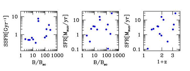
Figure 2: GRB host specific star formation rate (SSFR) and star formation rate (SFR) as a function of $B/B_{sc}$ (left and middle panels) and star formation rate as a function of $1+z$ (right panel).

As suggested by the measurements presented in the previous paragraph (see, e.g., Beck 2009) and also by larger fields of $0.5-18$ mG obtained in starburst galaxies with SFR $\sim 100M_{sun}$/yr (Robishaw, Quataert & Heiles 2008), galaxies with higher SFR tend to have higher global fields. The strength of the global field might be correlated with the field in the vicinity of the GRB, $B_{0}$. If this is the case, then simple shock-compression would remain a viable possibility for those bursts for which we have found large values of $B/B_{sc}$, if they reside within galaxies with high SFR. This idea is in the spirit of the work of Thompson, Quataert & Murray (2009), where they find that for supernova remnants (SNRs) fields larger than that due to shock-compression alone might not be needed for SNR in starbursts (nor for the average SNR in most normal spirals, although it might be needed for individual SNRs at particular moments of time).

We find that 13 GRBs out of our sample of 23 have their host galaxy SFR reported in Savaglio, Glazebrook & Le Borgne (2009). We present these values in Table 2 and plot them as a function of our values of $B/B_{sc}$ and as a function of redshift in Figure 2. There is no correlation between SFR and $B/B_{sc}$, nor SSFR (specific SFR) and $B/B_{sc}$. This does not support the idea that bursts with high values of $B/B_{sc}$ reside within galaxies with high SFR, and therefore they do require an amplification beyond shock-compression. This assumed however that the global galactic field is a proxy of the field in the vicinity of the GRB progenitor, $B_{0}$, which might not be the case with a progenitor that regulates the medium and the magnetic fields in its vicinity via winds or other mechanisms, or if the pre-shocked magnetic field is strongly amplified by instabilities that operate ahead of the shock (e.g., Milosavljević & Nakar 2006).

We also report the morphology of GRB host galaxies (Wainwright et al. 2007) in Table 2, using the notation in Savaglio et al. (2009). Only 10 GRBs of our sample of 23 have reported morphologies. Table 2 is presented in descending order of $B/B_{sc}$. There is no clear indication that GRBs hosted by galaxies of different morphologies have different strengths of $B/B_{sc}$. However, as mentioned above, global host galaxy properties might not represent the properties in the vicinity of the GRB. We emphasize that the ideas discussed in this paragraph and in the previous one are based on small number statistics and depend on the jet break time estimate. Larger samples in the future could be used to test them.

Using X-ray and optical data for a sample of GRB afterglows, Santana et al. (2014) have also constrained $\epsilon_{B}$: an upper limit with their X-ray sample and a measurement with their optical sample. We find that 4 GRBs: GRB 071003, GRB 080603A, GRB 090313 (in their optical sample), and GRB 100814A (in their X-ray sample), are common to our radio sample. Using the same assumptions, we find that our lower limits on $\epsilon_{B}$ for these 4 GRBs are consistent with the 3 measurements of $\epsilon_{B}$ (optical sample) and the upper limit on $\epsilon_{B}$ (X-ray sample) in Santana et al. (2014), showing that their methods and ours are consistent with each other. We note that our lower limits are only smaller by a factor of $\lower 2.0pt\hbox{$\,\buildrel\scriptstyle<\over{\scriptstyle\sim}\,$}3$ than the measurements/upper limits of these 4 GRBs. This means that for these 4 bursts the lower limits on $\epsilon_{B}$ are a good estimate of their actual values and, thus, require that $t_{j}\sim t_{p}^{obs}$. Only one of these 4 GRBs is in our subsample of GRBs with know jet break, GRB 090313. We find that our $\epsilon_{B}$ estimate using radio data is a factor of 100 larger than the one reported in Santana et al. (2014), since for this burst $t_{j}\ll t_{p}^{obs}$. This GRB has the highest $\epsilon_{B}$ value in Table 2 (and abnormally high compared with the rest of the sample). After inspecting its optical/X-ray afterglow, we find that its jet break time ($<1$ day) is based only on X-ray observations, since at this time the optical afterglow displays flares, and also contamination from a nearby source (Berger 2009, Mao et al. 2009, Melandri et al. 2010). Therefore, this jet break can be regarded as questionable, but we decided to keep it in Table 2 and Fig. 1.

Santana et al. (2014) find a weak correlation between $E$ and $\epsilon_{B}$. We do not find it in our radio sample with estimated jet break times, which might be due to the uncertainties in $t_{j}$. Finally, the mean/median value found for $B/B_{sc}\sim 30$ in our radio sample (for both the lower limits and the measurements) agrees very well with the value found in Santana et al. (2014), where they report $B/B_{sc}\sim 50$. We note that three very different methods (using radio, optical and X-ray data) yield consistent values of the level of amplification needed in GRB relativistic collisionless shocks.

Lemoine et al. 2013 have studied bursts with $>100$ MeV (detected by the Fermi satellite), X-ray, optical and radio data. They explain all these observations in the context of the external forward shock (see, e.g., Kumar & Barniol Duran 2009). However, they consider a decaying field behind the shock (Lemoine 2013), where the $>100$ MeV emission is produced by electrons close to the shock front, where $\epsilon_{B}\sim 10^{-2}-10^{-1}$ and the X-ray, optical, and radio emission is produced by electrons further downstream of the shock front, where $\epsilon_{B}\sim 10^{-6}-10^{-4}$. The latter value of $\epsilon_{B}$ is consistent with our obtained median of $\epsilon_{B}\sim 10^{-5}$ using radio data.

We note that the median value of $\epsilon_{B}$ found in this work, by assuming $n=1$ cm^-3 and a 20 per cent efficiency in producing the prompt emission gamma-rays, is a factor of $\sim 600$ smaller than the median value found in, e.g., Panaitescu & Kumar (2002), in which a detailed multiwavelength analysis of several of the bursts in our sample are presented. The main difference is that the median density found in Panaitescu & Kumar (2002) is $\sim 10$ times larger and the median efficiency is $\sim 70$ per cent. Also, the numerical pre-factor used in eq. (1) in Granot & Sari (2002) is much larger than the one used in Panaitescu & Kumar (2002), and since eqs. (2) and (3) depend on this pre-factor squared, then the effect is to lower $\epsilon_{B}$ considerably. A similar conclusion applies to our results regarding $B/B_{sc}$.

We would like to finish by comparing our values of $B/B_{sc}$ with the ones found for young shell-type supernova remnants (SNRs). There is some evidence for field amplification in Galactic SNRs with levels of $B/B_{sc}\sim 10-100$ at particular moments of time (e.g., Völk et al. 2002, Völk, Berezhko & Ksenofontov 2005, Berezhko, Ksenofontov & Völk 2006, see, also, recently, Castro et al. 2013). It is interesting to note that a similar level of amplification as the one presented in this work and in Santana et al. (2014) is observed in these systems. Taken at face value, this might indicate a common amplification mechanism in GRB relativistic afterglows and non-relativistic SNRs, which might even be found in other very different systems. We should caution, however, that the environment in the vicinity of the GRB explosion remains uncertain and every possible effort to characterize it should be made.

This work emphasizes the importance of radio afterglow observations in studying relativistic collisionless shocks. By using the simple method presented here, one can extract valuable information about the magnetic field behind the shock for GRBs, which have not been monitored extensively at other wavelengths to allow for a complete and detailed afterglow modeling. Radio monitoring of GRB afterglows at various wavelengths continues to be an indispensable tool in the study of collisionless shocks.

References

- [1]
- [2] Barniol Duran R., Kumar P., 2011a, MNRAS, 412, 522
- [3] Barniol Duran R., Kumar P., 2011b, MNRAS, 417, 1584
- [4] Berger E., 2009, GCN Circ. 8984
- [5] Berezhko E.G., Ksenofontov L.T., Völk H.J., 2006, A&A, 452, 217
- [6] Blandford R. D., McKee C. F., 1976, Phys. Fluids, 19, 1130
- [7] Beck R., 2009, in Strassmeier K.G., Kosovichev A.G., Beckman J.E., eds, Proc. IAU Symp. 259, Cosmic Magnetic Fields: From planets, to Stars and Galaxies. Cambridge Univ. Press, Cambridge, p. 3
- [8] Beck R., 2012, SSRv, 166, 215
- [9] Castro D., Lopez L.A., Slane P.O., Yamaguchi H., Ramirez-Ruiz E., Figueroa-Feliciano E., 2013, ApJ, 779, 49
- [10] Chandra P., Frail D.A, 2012, ApJ, 746, 156
- [11] Couch S.M., Milosavljević M., Nakar E., 2008, ApJ, 688, 462
- [12] Curran P.A., Evans P.A., de Pasquale M., Page M.J., van der Horst A.J., 2010, ApJ, 716, L135
- [13] De Colle F., Ramirez-Ruiz E., Granot J., Lopez-Camara D., 2012, ApJ, 751, 57
- [14] Frail D.A. et al., 2000, ApJ, 534, 559
- [15] Goodman J., MacFadyen A., 2008, J. Fluid Mech., 604, 325
- [16] Granot J., Sari R., 2002, ApJ, 568, 820
- [17] Inoue T., Asano K., Ioka K., 2011, ApJ, 734, 77
- [18] Kocevski D., Butler N., 2008, ApJ, 680, 531
- [19] Kumar P., Barniol Duran R., 2009, MNRAS, 400, L75
- [20] Kumar P., Barniol Duran R., 2010, MNRAS, 409, 226
- [21] Lemoine M., 2013, MNRAS, 428, 845
- [22] Lemoine M., Li Z., Wang X.-Y., 2013, MNRAS, 435, 3009
- [23] Leventis K., van Eerten H.J., Meliani Z., Wijers R.A.M.J., 2012, MNRAS, 427, 1329
- [24] Leventis K., van der Horst A.J., van Eerten H.J., Wijers R.A.M.J., 2013, MNRAS, 431, 1026
- [25] Liang E.-W., Racusin J.L., Zhang B., Zhang B.-B., Burrows D., 2008, ApJ, 675, 582
- [26] Mao J. et al. 2009, GCN Report 204.1
- [27] Medvedev M.V., Loeb A., 1999, ApJ, 526, 697
- [28] Melandri A. et al., 2010, ApJ, 723, 1331
- [29] Mészáros P., Rees M.J., 1993, ApJ, 405, 278
- [30] Mészáros P., Rees M.J., 1997, ApJ, 476, 232
- [31] Milosavljević M., Nakar E., 2006, ApJ, 651, 979
- [32] Mizuno Y., Pohl M., Niemiec J., Zhang B., Nishikawa K.-I., Hardee P.E., 2011, ApJ, 726, 62
- [33] Nakar E., Ando S., Sari R., 2009, ApJ, 703, 675
- [34] Paczyński B., Rhoads J.E., 1993, ApJ, 418, L5
- [35] Panaitescu A., 2005, MNRAS, 363, 1409
- [36] Panaitescu A., Kumar P., 2002, ApJ, 571, 779
- [37] Piran T., 2004, Rev. Modern Phys., 76, 1143
- [38] Racusin J.L. et al., 2009, ApJ, 698, 43
- [39] Rees M.J., Mészáros P., 1992, MNRAS, 258, 41P
- [40] Rhoads J.E., 1999, ApJ, 525, 737
- [41] Robishaw T., Quataert E., Heiles C., 2008, ApJ, 680, 981
- [42] Santana R., Barniol Duran R., Kumar P., 2014, ApJ, 785, 29
- [43] Sari R., Piran T., Narayan R., 1998, ApJ, 497, L17
- [44] Sari R., Piran T., Halpern, J.P., 1999, ApJ, 519, L17
- [45] Sari R., Esin A.A., 2001, ApJ, 548, 787
- [46] Savaglio S., Glazebrook K., Le Borgne D., 2009, ApJ, 691, 182
- [47] Soderberg A.M, 2006, ApJ, 650, 261
- [48] Sironi L., Goodman J., 2007, ApJ, 671, 1858
- [49] Thompson T.A., Quataert E., Murray N., 2009, MNRAS, 397, 1410
- [50] van Eerten H., MacFadyen A., 2013, ApJ, 767, 141
- [51] Völk H.J., Berezhko E.G., Ksenofontov L.T., Rowell G.P., 2002, A&A, 396, 649
- [52] Völk H.J., Berezhko E.G., Ksenofontov L.T., 2005, A&A, 433, 229
- [53] Wainwright C., Berger E., Penprase B.E., 2007, ApJ, 657, 367
- [54] Wijers R.A.M.J., Galama T.J., 1999, ApJ, 523, 177
- [55] Yost S.A., Harrison F.A., Sari R., Frail D.A., 2003, ApJ, 597, 459
- [56] Zhang W., MacFadyen A.I., 2009, ApJ, 698, 1261
- [57] Zhang W., MacFadyen, A.I., Wang P., 2009, ApJ, 692, L40
- [58]