The First Survey of X-ray Flares from Gamma Ray Bursts Observed by Swift: Temporal Properties and Morphology

Abstract

We present the first systematic investigation of the morphological and timing properties of flares in GRBs observed by Swift/XRT. We consider a large sample drawn from all GRBs detected by Swift, INTEGRAL and HETE-2 prior to 2006 Jan 31, which had an XRT follow-up and which showed significant flaring. Our sample of 33 GRBs includes long and short, at low and high redshift, and a total of 69 flares. The strongest flares occur in the early phases, with a clear anti-correlation between the flare peak intensity and the flare time of occurrence. Fitting each X-ray flare with a Gaussian model, we find that the mean ratio of the width and peak time is $\langle\Delta t/t\rangle=0.13\pm 0.10$, albeit with a large scatter. Late flares at times $>2000$ seconds have long durations, $\Delta t>300$ s, and can be very energetic compared to the underlying continuum. We further investigated if there is a clear link between the number of pulses detected in the prompt phase by BAT and the number of X-ray flares detected by XRT, finding no correlation. However, we find that the distribution of intensity ratios between successive BAT prompt pulses and that between successive XRT flares is the same, an indication of a common origin for gamma-ray pulses and X-ray flares. All evidence indicates that flares are indeed related to the workings of the central engine and, within the standard fireball scenario, originate from internal shocks rather than external shocks. While all flares can be explained by long-lasting engine activity, 29/69 flares may also be explained by refreshed shocks. However, 10 can only be explained by prolonged activity of the central engine.

1 Introduction

The advent of Swift (Gehrels et al., 2004) has brought substantial advances in our knowledge of GRBs including the discovery of the first afterglow (with a position known to several arcsec precision) of a short burst. Swift also brought on the definition of a possible third class of GRBs (Gehrels et al., 2006), the discovery of a smooth transition between prompt and afterglow emission (Tagliaferri et al., 2005; Vaughan et al., 2006; O’Brien et al., 2006), and the definition of a canonical X-ray light curve (Nousek et al., 2006; O’Brien et al., 2006; Zhang et al., 2006). The latter includes a steep early part ($\propto t^{-\alpha_{1}}$ with $3\lesssim\alpha_{1}\lesssim 5$, typically interpreted as GRB high-latitude emission), a flat phase ($0.5\lesssim\alpha_{2}\lesssim 1$, generally interpreted as due to energy injection into the external shock), and a last, steeper part ($1\lesssim\alpha_{3}\lesssim 1.5$, the only one observed by pre-Swift X-ray instruments), with the predicted $t^{-1}$ decay (see, also Wu et al. 2005). Sometimes, a further steepening is detected after the normal decay phase, which is consistent with a jet break (Zhang et al., 2006).

What may be the most surprising discovery is the presence of flares in a large percentage of X-ray light curves. Flares had been previously observed in GRB 970508 (catalog ) (Piro et al., 1999), GRB 011121 (catalog ) and GRB 011211 (catalog ) (Piro et al., 2005). Piro et al. (2005) suggested that the X-ray flares observed in the latter two events were due to the onset of the afterglow, since the spectral parameters of these flares were consistent with those of their afterglow. Starting from XRF 050406 (catalog ) (Burrows et al., 2005b; Romano et al., 2006b), GRB 050502B (catalog ) (Falcone et al., 2006), and GRB 050607 (catalog ) (Pagani et al., 2006), we have learned that flares can be considerably energetic and that they are often characterized by large flux variations. Indeed, the flare fluences can be up to 100% of the prompt fluence and the flare fluxes, measured with respect to the underlying continuum, $\Delta F/F$, can vary in very short timescales $\Delta t/t_{\rm peak}$ ($\Delta F/F\sim 6$, 500 and 25, $\Delta t/t_{\rm peak}\ll 1$, $\sim 1$, $\sim 1$ in XRF 050406, GRB 050502B and GRB 050607, respectively, where $\Delta t$ measures the duration of the flare and $t_{\rm peak}$ is measured with respect to the trigger time). Furthermore, detailed spectral analysis has proven that these flares are spectrally harder than the underlying continuum (Burrows et al., 2005b; Romano et al., 2006b; Falcone et al., 2006). In particular, they follow a hard-to-soft evolution, which is reminiscent of the prompt emission (e.g. Ford et al. 1995). The spectra of the flares in GRB 050502B (Falcone et al., 2006) are better fit by a Band function (Band et al., 1993, which is the standard fitting model for GRB prompt emission), than by an absorbed power law (which usually suffices for a standard afterglow). Very often multiple flares are observed in the same light curve, with an underlying afterglow consistent with having the same slope before and after the flare. Finally, GRB 050724 (catalog ) (Barthelmy et al., 2005f; Campana et al., 2006) and GRB 050904 (catalog ) (Cusumano et al., 2006) have demonstrated that flares happen in short GRBs as well as long ones, at low and very high redshift (the record being held by GRB 050904 at $z=6.29$).

The picture that the early detections of flares have drawn was described by Burrows et al. (2006) and Chincarini et al. (2006, and references therein), and a few conclusions were derived, albeit based on a small sample of objects. The presence of an underlying continuum consistent with the same slope before and after the flare (GRB 050406, GRB 050502B) seems to rule out external shocks models, since no trace of an energy injection can be found; the large observed $\Delta F/F$ cannot be produced by synchrotron self-Compton in the reverse shocks; the very short timescales $\Delta t/t_{\rm peak}<1$ also generally rule out external shocks, unless very carefully balanced conditions are met (e.g., Kobayashi et al., 2007); furthermore, the flare spectral properties (harder than the underlying afterglow, evolving from hard to soft) indicate a different physical mechanism from the afterglow, and possibly the same as the prompt one.

In this work we present the first comprehensive temporal analysis of all GRBs observed by the X-ray Telescope (XRT, Burrows et al. 2005a)–both long and short, independently of whether they are GRBs, X-ray Rich (XRR) or X-ray Flashes (XRF, Heise et al. 2001) at low and high redshift–that showed flares in their X-ray light curves. We assess whether the evidence for prolonged engine activity accumulated on the first observed flares survives statistical investigation and discuss the case that flares are indeed related to the workings of the central engine. We also present the results of a cross-check analysis between X-ray flares and pulses detected by the Burst Alert Telescope (BAT, Barthelmy et al. 2005e) in the gamma-ray prompt emission. A second paper (Falcone et al., 2007) will study the same sample from the spectroscopic point of view, in a natural complement to this work.

This paper is organized as follows. In §2 we describe our GRB sample and in §3 the data reduction procedure; in §4 we describe our XRT data analysis and in §5 our cross-check analysis between X-ray flares and pulses detected by BAT in the gamma-ray prompt emission. In §6 we present our main results and in §7 we discuss our findings. Throughout this paper the quoted uncertainties are given at 90% confidence level for one interesting parameter (i.e., $\Delta\chi^{2}=2.71$) unless otherwise stated. Times are referred to the BAT trigger $T_{0}$, $t=T-T_{0}$, unless otherwise specified. The decay and spectral indices are parameterized as $F(\nu,t)\propto t^{-\alpha}\nu^{-\beta}$, where $F_{\nu}$ (erg cm^-2 s^-1 Hz^-1) is the monochromatic flux as a function of time $t$ and frequency $\nu$; we also use $\Gamma=\beta+1$ as the photon index, $N(E)\propto E^{-\Gamma}$ (ph keV^-1 cm^-2 s^-1).

2 Sample definition

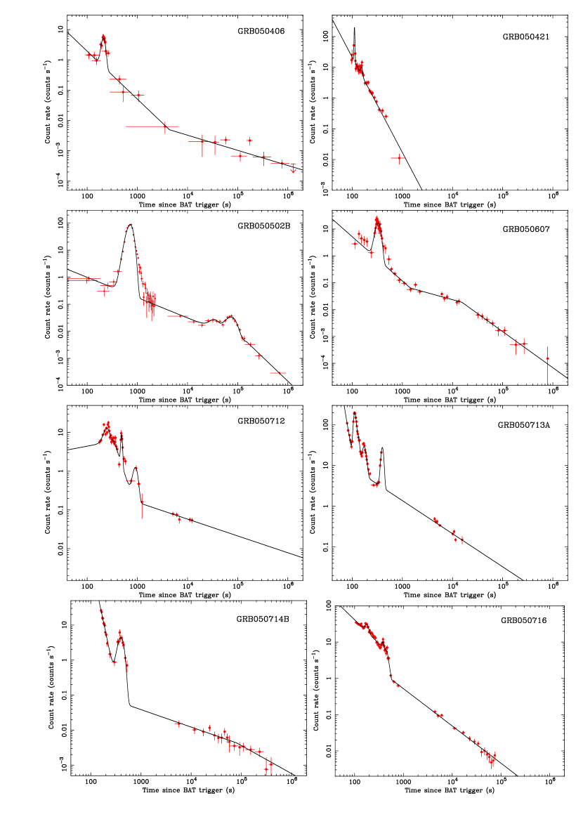
Figure 1: Flare fits. The thick line is the best fit to the XRT data (filled circles) with a (multiply-)broken power law plus a number of Gaussians (see Table 3 for the fit parameters). The continumm and Gaussian parameters are reported in Table 2 and Table 3, respectively. For GRB 060124 we considered the prompt and afterglow portion of the light curve separately.

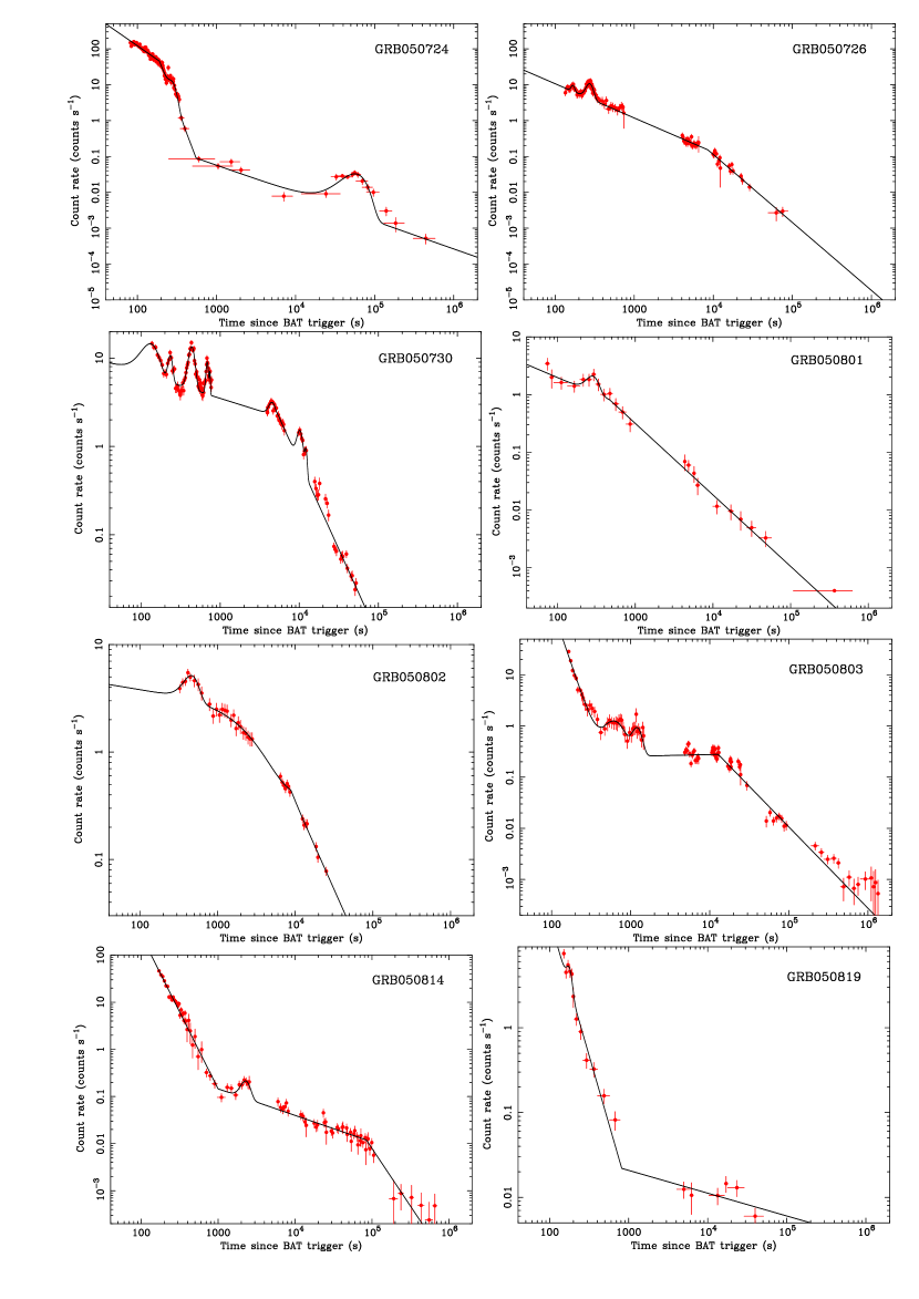
Figure 1: Continued.

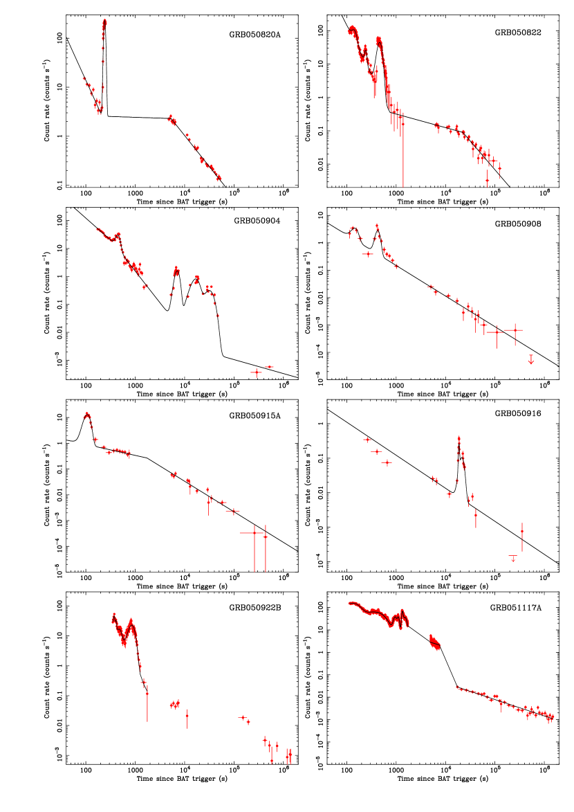
Figure 1: Continued.

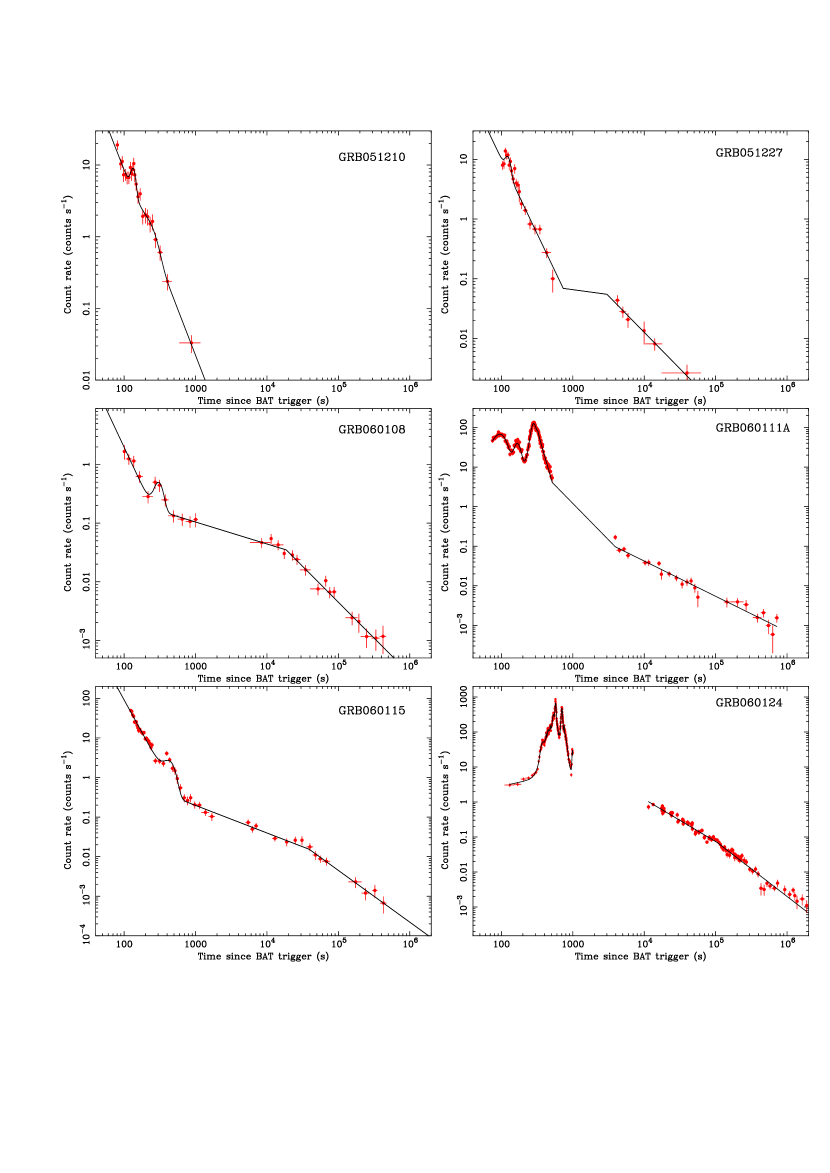
Figure 1: Continued.

We considered all GRBs detected by Swift, INTEGRAL and HETE-2, between the Swift launch and 2006 January 31 (119 events) for which XRT obtained a position (99). We then examined all light curves searching for large scale activity in excess of the underlying power-law light curve (flares). We defer a detailed analysis of small scale and small frequency variability, sometimes referred to as “flickering” to a later paper. None of the INTEGRAL- or HETE-2–triggered bursts showed any flares although we note that these bursts were observed by XRT much later than the Swift-triggered ones. As will be discussed in §4.4, where we investigate the sample biases in depth, we evaluate the completeness of our sample with a large set of simulations. We established that our flare sample can be considered complete with respect to faint flares only at late times (typically $10^{3}$ seconds after the trigger). In Table The First Survey of X-ray Flares from Gamma Ray Bursts Observed by Swift: Temporal Properties and Morphology we list all the GRBs that were selected for the analysis along with their redshifts (when available, i.e., for 9 of them), $T_{90}$s, and BAT fluences. This is what we shall refer to as our “full” sample, consisting of 33 GRBs, on which we attempted the timing analysis described in §4. The light curves of the full sample are shown in Fig. 1.

Some light curves, however, were not fit for the full analysis. For instance, although joint analysis of BAT and XRT data on GRB 050219A (Goad et al., 2006) showed a simultaneous flare (hence its inclusion in our sample), the portion of the flare that was observed with XRT was not long enough to fully characterize it. In the same manner, a handful of events (GRB 050826, GRB 051016B, GRB 060109) which are included in our full sample because they showed either low-signal late-time flares or a flattening in the XRT light curve, were excluded from a full analysis because of the low statistics obtained. All these special cases are reported in Table The First Survey of X-ray Flares from Gamma Ray Bursts Observed by Swift: Temporal Properties and Morphology in italics. After these exclusions, we defined our “restricted” sample, which consists of 30 GRBs on which we succeeded in performing our full analysis.

We note that our restricted sample differs from the one of Falcone et al. (2007), because of different requirements for the analysis. As an example, for GRB 050820A Falcone et al. (2007) could perform detailed spectroscopic analysis of the flare portion observed by XRT, but our full timing analysis was not applicable.

3 Data Reduction

The XRT data were first processed by the Swift Data Center at NASA/GSFC into Level 1 products (event lists). Then they were further processed with the XRTDAS (v1.7.1) software package, written by the ASI Science Data Center (ASDC) and distributed within FTOOLS to produce the final cleaned event lists. In particular, we ran the task xrtpipeline (v0.9.9) applying calibration and standard filtering and screening criteria. An on-board event threshold of $\sim$0.2 keV was applied to the central pixel of each event, which has been proven to reduce most of the background due to either the bright Earth limb or the CCD dark current (which depends on the CCD temperature).

The GRBs in our sample were observed with different modes, which were automatically chosen, depending on source count rates, to minimize pile-up in the data (Hill et al., 2004). For the GRBs observed during the calibration phase, however, the data were mainly collected in Photon Counting (PC) mode, and pile-up was often present in the early data. Furthermore, for a few, especially bright GRBs (which were observed after the Photo-Diode (PD) mode was discontinued due to a micrometeorite hit on the CCD) the Windowed Time (WT) data were piled-up, as well. Generally, WT data were extracted in a rectangular 40$\times$20-pixel region centered on the GRB (source region), unless pile-up was present. To account for this effect, the WT data were extracted in a rectangular 40$\times$20-pixel region with a region excluded from its centre. The size of the exclusion region was determined following the procedures illustrated in Romano et al. (2006a). To account for the background, WT events were also extracted within a rectangular box (40$\times$20 pixels) far from background sources.

The PC data were generally extracted from a circular region with a 30-pixel radius. Exceptions were made for bright sources, which required a $>30$-pixel radius, and for faint sources, which required a smaller radius in order to maintain a high signal-to-noise ratio. When the PC data suffered from pile-up, we extracted the source events in an annulus with a 30-pixel outer radius and an inner radius, depending on the degree of pile-up as determined via the PSF fitting method illustrated in Vaughan et al. (2006). PC background data were also extracted in a source-free circular region.

For our analysis we selected XRT grades 0–12 and 0–2 for PC and WT data, respectively (according to Swift nomenclature; Burrows et al. 2005a). To calculate the PSF losses, ancillary response files were generated with the task xrtmkarf within FTOOLS, and account for different extraction regions and PSF corrections. We used the latest spectral redistribution matrices in the Calibration Database maintained by HEASARC.

From both WT and PC data, light curves were created in the 0.2–10 keV energy band using a criterion of a minimum of 20 source counts per bin, and a dynamical subtraction of the background. Therefore, in our sample, each light curve was background-subtracted, and corrected for pile-up, vignetting, exposure, and PSF losses.

4 Data Analysis

The first goal of this work was to obtain a quantitative assessment of flare characteristics. We thus set to measure statistical parameters such as the ratio of the flare duration to the time of occurrence $\Delta t/t$, the power-law decay slope $\alpha_{\rm fall}$, the decay to rise ratio $\Delta t_{\rm fall}/\Delta t_{\rm rise}$, the flare energetics, and the flare to burst flux ratio. Different approaches suited the data best, depending on the flare statistics, as we outline below.

4.1 Equivalent widths

We calculated the equivalent width of the flares defined as $EW=\int\frac{F_{\rm observed}(t)-F_{\rm continuum}(t)}{F_{\rm continuum}(t)}\,dt$, where $F_{\rm continuum}(t)$ describes the assumed shape of the continuum light curve underneath the flare (the local power law “underlying continuum”) and $F_{\rm observed}(t)$ is the observed light curve, i.e., the combination of the continuum and flare (the analytical fits to the continua are described in detail in §4.2 and their parameters reported in Table 2). The equivalent width (expressed in units of seconds, as reported in Table 3 column 6) represents the time needed for integration of the continuum to collect the same fluence as of the flare and it can give us a first indication of the lowest fluence we are able to measure for a flare. Indeed, the faintest equivalent width measured, on a rather weak afterglow with XRT fluence of $\sim 1.3\times 10^{-8}$ erg cm^-2 light curve, is 7.9 s in a small flare detected in GRB 050819. At the other extreme of the $EW$s is GRB 050502B, where we detect two flares, both characterized by large $EW$s. The first one is extremely bright and indeed has a fluence that is larger than the fluence of the underlying continuum light curve ($1.43\times 10^{-6}$ erg cm^-2 and $1.23\times 10^{-6}$ erg cm^-2, respectively). Even though (see §4.4) our completeness for faint flares is somewhat limited at early times, this may be an indication that the flare is generally stronger than the continuum light curve and possibly an unrelated phenomenon.

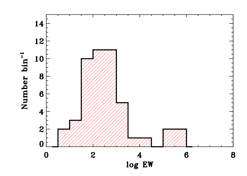
Figure 2: Distribution of the equivalent width (in seconds) of the flares. The times are are not corrected for redshift.

Our ability to measure $EW$s is limited by the discrete sampling of the light curves as well as the relative faintness of the flares, therefore we could only obtain $EW$s for 48 flares. Figure 2 shows the distribution of the $EW$s for our sample.

4.2 $\Delta t/t$ from Gaussian fits

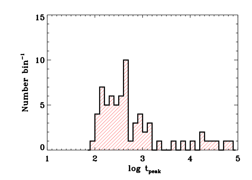
Figure 3: Distribution of the peak times of the flares in excess of the canonical XRT light curve. The times are referred to the trigger time, and are not corrected for redshift.

The simplest analytical characterization of the flare morphology is obtained by adopting a multiply-broken power law to model the underlying continuum, and a number of Gaussians to model the superimposed flares. We adopted the following laws for the continuum, i) simple power law: $F(t)=Kt^{-\alpha_{1}}$, ii) broken power law: $F(t)=Kt^{-\alpha_{1}}$ for $t<t_{\rm b1}$ and $F(t)=K\,t_{\rm b1}^{-\alpha_{1}}\,(t/t_{\rm b1})^{-\alpha_{2}}$ for $t>t_{\rm b1}$, iii) doubly-broken: $F(t)=Kt^{-\alpha_{1}}$ for $t<t_{\rm b1}$ and $F(t)=K\,t_{\rm b1}^{-\alpha_{1}}\,(t/t_{\rm b1})^{-\alpha_{2}}$ for $t_{\rm b1}<t<t_{\rm b2}$, $F(t)=K\,t_{\rm b1}^{-\alpha_{1}}\,(t_{\rm b2}/t_{\rm b1})^{-\alpha_{2}}\,(t/t_{\rm b2})^{-\alpha_{3}}$ for $t>t_{\rm b2}$, and so on, where $t_{\rm b1}$ and $t_{\rm b2}$ are the times of the breaks. For our flares, we iteratively added as many Gaussians as required to accommodate the $\chi^{2}$ locally around each flare. The best-fit model parameters for each component (continuum and flares) were derived with a joint fit and are reported in Table 2 (continuum parameters) and Table 3 (flare parameters, columns 2–4). Column 5 of Table 3 reports flare peak fluxes measured with respect to the underlying continuum, or $\Delta F/F$). The full gallery of fits is illustrated in Fig. 1. In Fig. 3 we show the distribution of the peak times (i.e., the Gaussian peaks).

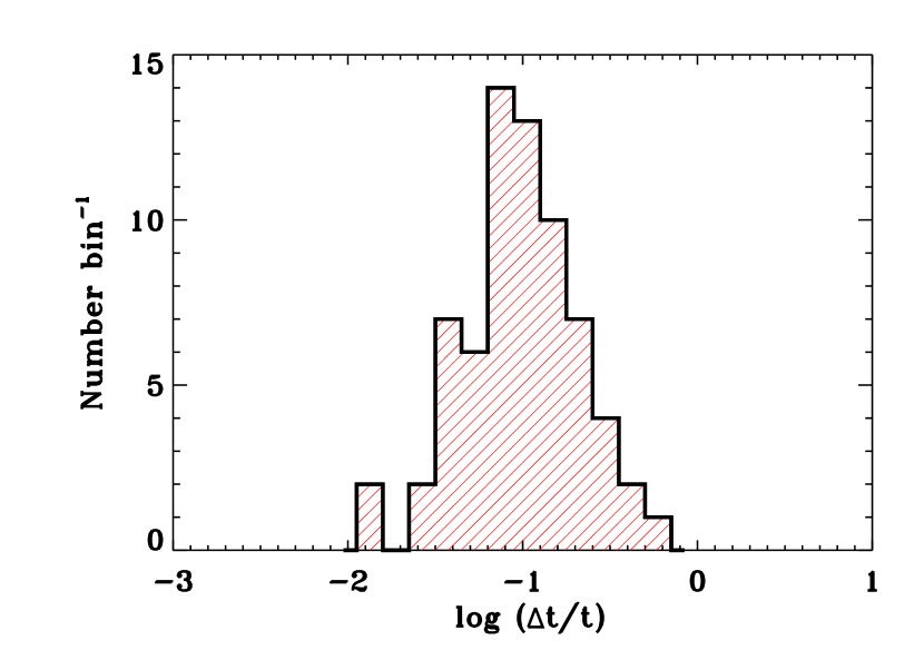
Figure 4: Distribution of the ratio of the flare duration vs. the time of occurrence $\Delta t/t$, obtained fitting the flares with Gaussian models (§4.2), where $\Delta t$ is the width of the Gaussian and $t$ is the Gaussian peak time. This ratio is independent of redshift.

Based on these fits, we calculated $\Delta t/t$ for each flare, adopting the Gaussian width ($\sigma$) and peak $t_{\rm peak}$ as $\Delta t$ and $t$, respectively, where $t_{\rm peak}$ ranges between 95 s and $\sim 75$ ks. We do not include the Gaussian fits for GRB 060124 for sake of homogeneity of the sample, since the XRT data include the prompt phase (Romano et al. 2006a). Our ability to fit flares with Gaussians is less affected by discrete sampling of the light curves than for the $EW$ determination, but it still suffers from the faintness of the flares; therefore we obtained fits for 69 Gaussian-modeled flares. In Fig. 4, we show the distribution of the $\Delta t/t$, which peaks at $0.13$, and which yields a mean value of $\langle\Delta t/t\rangle=0.13\pm 0.10$. An assessment of selection effect that may affect this result is reported in §4.4.

4.3 Decay slopes, rising and decaying times from more realistic models

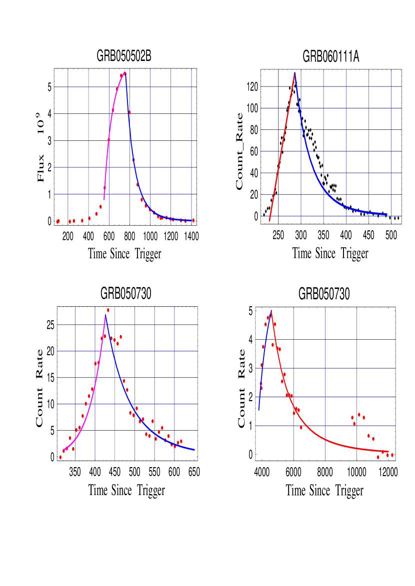
Figure 5: Different flare morphologies as represented by GRB 050502B, GRB 050730, and GRB 060111A. For GRB 050730 different flares are best fit by different laws (two power laws for the first, and an exponential rise followed by a power-law decay for the second one.)

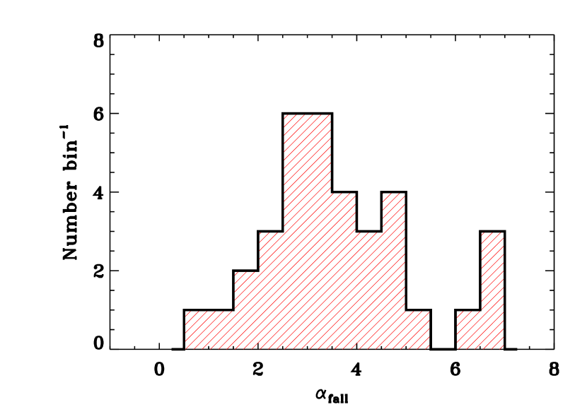
Figure 6: Distribution of the decay slope $\alpha_{\rm fall}$ computed using as initial time the point where the flux is 1% of the peak (see §4.3).

Flare profiles can be quite complex. As an example, in Fig. 5 we show the light curves of GRB 050730, in which different flares are best fit by different laws (two power laws for the first, and an exponential rise followed by a power-law decay for the second one), of GRB 050502B (first flare), and GRB 060111A. A more realistic description of the flare profile should therefore account for the skewness observed in many flares as well as different rising and falling slopes and times, which we indicate with $\alpha_{\rm rise}$, $\alpha_{\rm fall}$, $\Delta t_{\rm rise}$, and $\Delta t_{\rm fall}$, respectively. Such a fit can be performed with power laws ($F(t)\propto(t-t_{0})^{-\alpha}$), in which case it is critical to define the reference time $t_{0}$. In practice, for $t_{0}$ we consider the peak time as well as the times, before and after the peak, when the flare profile deviates significantly from the continuum fit: $\Delta t_{\rm rise}=t_{\rm peak}-t_{1}$, $\Delta t_{\rm fall}=t_{2}-t_{\rm peak}$, where $t_{1}$ and $t_{2}$ are the times when the flare emission (fitted in this case by a Gaussian) crosses the fraction $f$ of the flare peak emission on either side of the peak. For the calculation of the decay slopes, we chose $f=0.01$. As for the previous fits (4.1, 4.2), our procedure requires a power law continuum beneath each flare. The values of $\alpha_{\rm fall}$ we computed for this sample (consisting of 35 flares) are reported in Table 3 (column 7) and their distribution is shown in Fig. 6. We derive $\langle\alpha_{\rm fall}\rangle=3.54$ with standard deviation of $\sigma=1.50$. We note that our choice of $f=0.01$ was an operative decision; using a different definition for $t_{1}$ and $t_{2}$, the measure of the slope decay changes. For instance, for the large flare in GRB 050502B we obtain $\alpha_{\rm fall}=6.32$, 5.58, and 5.20 for $f=0.01$, 0.05 and 0.10, respectively. This shows how critical the definition of $t_{1}$ and $t_{2}$ is in measuring the decay slope that describes the temporal behaviour of a burst or flare.

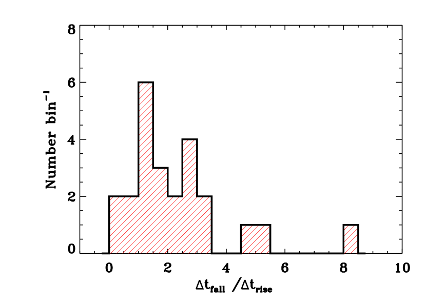
Figure 7: Distribution of $\Delta t_{\rm fall}/\Delta t_{\rm rise}$ obtained fitting the flares with power-law and exponential models. These ratios are independent of redshift.

The quantities $\Delta t_{\rm rise}$ and $\Delta t_{\rm fall}$ are in themselves quite interesting, since, as is well known from the work of Norris et al. (1996) and from the simulations by Daigne & Mochkovitch (1998), the observed bursts, which are due to the internal shocks, present a Fast-Rise Exponential-Decay (FRED) shape with a ratio $\Delta t_{\rm fall}/\Delta t_{\rm rise}=3.4$. We calculated $\Delta t_{\rm rise}$ and $\Delta t_{\rm fall}$ for our sample defining them in terms of $f=0.05$, by assuming the underlying power law continuum beneath the flares, and performing a separate fit to the rising and decaying part of the flare light curve. While for the decaying part we always used a power law, we found that in many instances the best fit to the rising part was obtained with an exponential. Using these fits, we calculated $\tau_{90}$ (the time defined by $f=0.05$) and the ratio $\Delta t/t$ adopting $\Delta t=\tau_{90}$ and $t=t_{\rm peak}$. Table 3 reports $\tau_{90}$, $\Delta t_{\rm fall}/\Delta t_{\rm rise}$, $\Delta t/t$ (columns 8–10), while Fig. 7 shows the distributions of $\Delta t_{\rm fall}/\Delta t_{\rm rise}$.

4.4 Selection effects

As stated above, our ability to measure statistical quantities from the light curves critically depends on both the discrete sampling of the light curves as well as the actual intensity of the flares with respect to the continuum beneath them. In this section we present our considerations on the biases that may affect our analysis and their effect on our results. One of the first difficulties comes from the blending of flares, which causes the $EW$, $\Delta t$, $\Delta t/t$, to be overestimated. Our result of low $\Delta t/t$ is thus an upper limit on the intrinsic sharpness of flares.

4.4.1 Time resolution and low-earth orbit biases

The time resolution of our observations, which decreases logarithmically during the XRT afterglow follow-up, is the first critical factor. Typically, at the beginning of the XRT light curve the sampling is quite good, but if the flare duration is of the order of the time it takes it to fade, then it will not be possible to recognize it as such, and it will be interpreted as a steep power law, instead. This was often observed in the early XRT light curves, as reported by Tagliaferri et al. (2005) and O’Brien et al. (2006), and it is partially related to the short but finite time (usually $>60$ s) it takes Swift to re-point to the GRB. On the other hand, at the end of the XRT light curve, the sampling also degrades because of the long integration required to achieve sufficient $S/N$, so that flares shorter than the integration time are smeared out and consequently, except for the brightest ones, their resulting average count rate drops below the detection threshold.

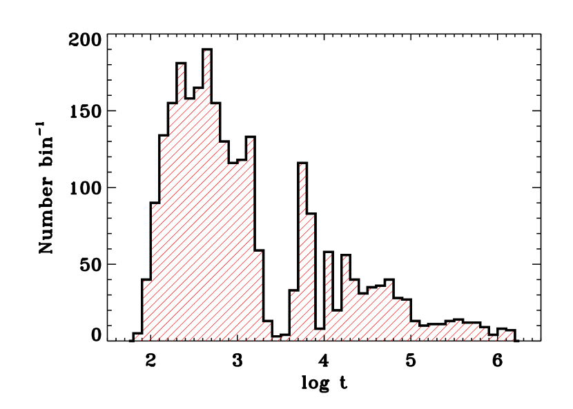
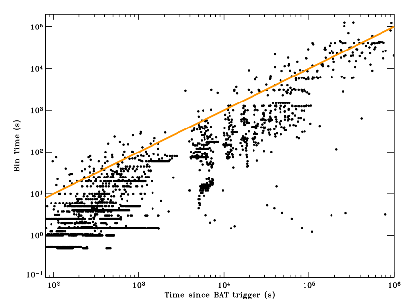
Figure 8: (left): Distribution of observing times. The gap at $\log t\sim 3.5$ is due to observing constraints (end of the first orbit). (right): Time resolution (BT) as a function of the time since the BAT trigger. The solid curve corresponds to BT$/t=0.1$ and lies above the large majority of the data points.

Due to Swift’s low-earth orbit, the data are not collected in a continuous way, but in portions of an orbit that last less than an hour. This is illustrated in Fig. 8 (left), which represents the distribution of the observing times relative to the BAT trigger, of all the light curves in our sample. For each observation of the light curve, we estimated the time, which we shall refer to as bin time (BT), within which the counts were accumulated in order to have a $S/N>3$. For $t>10^{4}$ s the BT will generally include data from consecutive orbits. In Fig. 8 (right), we show the time resolution (BT) as a function of the time since the BAT trigger, as well as the curve that corresponds to BT$/t=0.1$ and lies above the large majority of the data. It indicates that the instrumental resolution $BT/t=(\Delta t/t)_{S/N=3}$ is in most cases significantly better than $\Delta t/t\approx 0.1$ and is often even better than 0.01. In other words, our data are not biased against $\Delta t/t\lesssim 0.1$.

4.4.2 Biases in the sample definition criteria

In order to evaluate the completeness of our sample we tested the sample definition criteria against selection effects by means of simulations.

First of all, for each flare in our sample, we evaluated the signal to noise (S/N) ratio as the ratio between the fluence of the flare and the continuum calculated in the time interval [$-1\sigma$,$+1\sigma$], where $\sigma$ is the Gaussian width. The minimum detected S/N is 5. Then, to simulate our procedure, we first calculated the median continuum light curve from the whole data sample. This median light curve at late times is well described by a single power law with $\alpha_{\rm median}=1.1$. On top of that we summed a Gaussian flare with the 3 parameters randomly chosen and uniformly distributed over large intervals which fully contain the real data parameter values. From this parent distribution we generated a collection of photons. Finally we reconstructed the light curve, using the same procedure as we used for the real data. In this way we realistically reproduced a typical observed light curve. The only significant difference is that when we simulated, we assumed a continuous observation, whereas the real observation is split in different orbits. However, as discussed in the previous section, this assumption does not affect our conclusions. We repeated the test 14000 times in order to have a statistically significant sample of simulated light curves. For each randomly generated peak we calculated the S/N ratio and we flagged it as identified when its S/N ratio exceeded the value of 5 and, at the same time, at least 3 points in the light curve lay more than 2-$\sigma$ above the continuum. In Fig. 9 we plot the results of the simulations in the ($t$, $\Delta t$) plane. For each ($t$, $\Delta t$) value we could assign a detection probability; the points are the real data. We note that at early times our sample data lie in the region with low detection probability. This is clearly an effect of the significance threshold: at the beginning, the afterglow is brighter, the absolute level of the noise is high and a flare can be detected only if it is bright enough to have significance above the threshold. Given the median continuum light curve, our simulations show that if flare has a $\sim$90% detection probability at 10 ks, at 300s it will have a $\sim$ 30% detection probability. At late times the simulation results show that the detection probability decreases with smaller $\Delta t$ (bottom-right corner of the plot): this is an effect of threshold set as the minimum number of photons per bin of the light curve. At larger times the light curve has a sparse sampling and a faint and narrow flare produces only few bins over the continuum. Our simulations also show that, in the region of the plane defined by $\Delta t/t>2\times 10^{-3}$ and by $t>10^{4}$ s, the detection probability is uniformly larger than 90%. In Fig. 9 we also plotted the line $\Delta t=t$ over which we do not expect to find any flare. Comparing our sample with the simulation probability map we conclude that we do not find narrow flares at large $t$ in the areas of the parameter plane where we have very high detection probability. Therefore, although we cannot evaluate the completeness of our sample at early times, from our simulations we can firmly conclude that the lack of narrow flares at late times (typically $10^{3}$ s) is not due to incompleteness.

5 XRT flares vs. BAT pulses

We investigated if there is a clear link between the properties of the pulses detected in the gamma-ray burst profile by BAT in the 15–350 keV band and the X-ray flares as detected by XRT.

In order to define a procedure to select and characterize BAT pulses, we used an adapted version of the criterion defined by Li & Fenimore (1996): we started from the 64-ms mask-tagged light curve extracted following the standard BAT pipeline and searched for those bins whose count rates exceed $m$ contiguous bins by $n\sigma$ on both sides. We applied this procedure with three different combinations of $(m,n)$: $(5,3)$, $(3,4)$, and $(1,5)$ and to all of the curves with multiple binning times from 64 ms to 32 s, taking into account all of the possible shifts at a given binning time. This choice proved to be effective in catching different pulses clearly detected by visual inspection. We assessed the false positive rate of pulses so detected with a Monte Carlo test: we took the number of 64-ms bins of the longest GRB light curve available and simulated 100 synthetic light curves with constant signal, whose count rates were affected by Gaussian noise. We applied the same procedure to these 100 synthetic light curves and found 8 false pulses. We then estimated the average false positive rate as of 0.08 fake pulses for each GRB light curve. As we collected 28 GRBs with a complete BAT light curve [GRB 050820A was ignored because Swift entered the South Atlantic Anomaly (SAA) before the gamma-ray prompt emission ceased], we expect about 2 false pulses. We detected 46 pulses distributed in 28 gamma-ray profiles, so we can safely assume a negligible contamination of the gamma-ray pulses sample due to statistical fluctuations.

Table 4 shows the results of the BAT pulses quest, which identified 46 pulses out of 28 GRBs. For each pulse, columns 1–6 report: (1) the GRB name it belongs to, (2) the ordinal number of the pulse within the GRB, (3) the binning time used to detect the pulse (which also corresponds to the uncertainty on the peak time), (4) the peak time, (5) the peak rate (counts s^-1), (6) error on the peak rate (counts s^-1).

We do not find any clear correlation between the number of gamma-ray pulses and the number of X-ray flares. Column (1) in Table 5 reports the number of gamma-ray pulses found in a given burst; column (2) the number of X-ray flares, and column (3) reports the number of GRBs with that combination of numbers of pulses and flares. The most common case is when the burst exhibits one single pulse followed by one, or two X-ray flares.

We tested whether there is any statistical evidence that GRBs with many/few pulses are more likely to have many/few X-ray flares. Let $n_{\gamma}$ and $n_{\rm x}$ be the number of gamma-ray pulses and of X-ray flares of a given burst, respectively. We split the sample in two classes in two ways: those with $n_{\gamma}\geq 2$ (“many pulses”; 10 GRBs) and those with $n_{\gamma}<2$ (“few pulses”; 18 GRBs); likewise, those with $n_{\rm x}\geq 3$ (“many flares”; 11 GRBs) and those with $n_{\rm x}<3$ (“few flares”; 17 GRBs). From Table 5 one counts 5 bursts with both many pulses and many flares. In the assumption of no correlation between the number of pulses and the number of flares, the probability of choosing randomly $n\geq 5$ bursts with many pulses out of 11 bursts with many flares is about 35%: i.e. given a burst with many flares, nothing can be inferred about its number of pulses. Similarly, the probability of selecting $n\geq 5$ bursts with many flares out of 10 bursts with many pulses is 32%: i.e. given a burst with many pulses, nothing can be inferred about its number of flares. We also tried to split the sample with different combinations of thresholds on $n_{\gamma}$ and $n_{\rm x}$, but no statistically significant correlation has come out. Furthermore, we compared the distributions of the numbers of pulses derived for the two populations, i.e. those with few flares and those with many flares. A Kolmogorov-Smirnov (KS) test shows no difference between the two subsets, with 88% probability that they have been drawn from the same population. Likewise, we compared the distributions of the numbers of flares derived from splitting the sample between GRBs with few and many pulses, respectively. According to the KS test, we cannot reject that the two distributions are the same at 99% confidence level. We conclude that one cannot infer anything about the number of X-ray flares from the number of gamma-ray pulses and vice versa.

We also compared the distribution of the numbers of pulses with that of the numbers of flares and a KS test does not prove any significantly different origin (30% probability of having been drawn from the same distribution).

We also sought any possible correlation between the intensity of the pulses and properties of the flares as well as between the peak times of either class. To this aim, for each GRB in Table 6 we grouped the following pieces of information: columns 1–3 report the GRB name, the number of BAT pulses $n_{\gamma}$ and the number of X-ray flares $n_{\rm x}$, respectively. From column (4) up to column (12) the correspondent times are reported (referred to the BAT trigger time): the first $n_{\gamma}$ refer to the BAT pulses, while the remaining $n_{\rm x}$ refer to the X-ray flares.

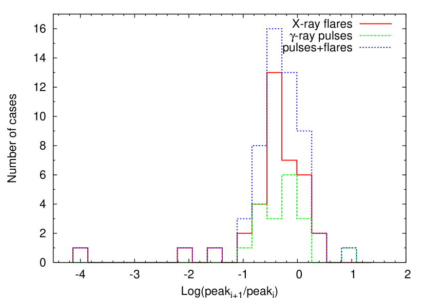
Figure 11: Distribution of the ratio between the peaks of two successive events: X-ray flares (red), gamma-ray pulses (green), both classes (blue).

For either class we considered those bursts with at least two events (i.e., either two pulses or two flares). We searched for any correlation between the quiescent time (between two successive pulses, or between two flares) and the peak brightness of the following event, but our search was unsuccessful. We also studied the relation between quiescent time and the ratio of the following peak, ${\rm peak}_{i+1}$ over the preceding peak, ${\rm peak}_{i}$. Figure 10 shows two interesting results: firstly, there is no clear dependence of this ratio on the quiescent time for both classes. Secondly, the distribution of ratios derived from the X-ray flares is consistent with that of the gamma-ray pulses. In particular, if we merge the two sets of ratios, this is consistent with a log-normal distribution with mean value $<\log{({\rm peak}_{i+1}/{\rm peak}_{i})}>=-0.258$ and $\sigma_{\rm log}=0.68$ (see Fig. 11). If we ignore the two points due to X-ray flares with the lowest ratio (see Fig. 10), the mean value and standard deviation turn out to be $-0.157$ and 0.41, respectively (shown in Fig. 10).

We therefore conclude that the relation between successive pulses and between successive flares is the same: in particular, on average the next event has a peak $10^{-0.157}\simeq 0.7$ times as high as the preceding, while the scatter is between 0.3 and 1.8. This further piece of evidence points to a common origin for gamma-ray pulses and X-ray flares.

6 Results

In this section we explore possible correlations between the parameters derived in the analysis and summarize our findings.

6.1 Gaussian peak time–intensity correlation

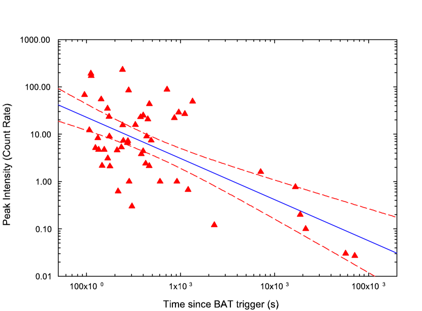
Figure 12: Gaussian peaks of the flares as a function of time. The solid line is the best fit, while the dashed lines correspond to 95% confidence limits.

We tested for a correlation between the Gaussian peak intensity and the peak position (s since the BAT trigger). As shown in Fig. 12, the correlation is strong, with a Spearman rank coefficient $r_{\rm s}=-0.539$ (number of points $N=63$, and null hypothesis probability nhp$=5.24\times 10^{-6}$). However, it can be argued that this correlation is driven by the flares at late times and that there is large scatter for $t<10^{3}$ s. In this light, this would be an indication that the mechanism producing the flares holds no memory of when the trigger time occurred. Therefore, the only firm conclusion we can draw is that the late flares have a peak intensity which is less than the early ones and coupling this with the $\Delta t$ results (see §4.2) we infer that late flares have a lower peak intensity but last much longer so their fluence can be very large.

6.2 $EW$ correlations

We find a strong correlation between the equivalent width and the time of the occurrence of the flare, $t_{\rm peak}$, ($r_{\rm s}=0.729$, $N=48$, nhp$=4.1\times 10^{-9}$) which is mostly due to the large dynamical range in $t_{\rm peak}$ values. Indeed, we find no correlation of $EW/t_{\rm peak}$ with $t_{\rm peak}$. There is also no correlation between $EW/t_{\rm peak}$ and $\Delta t/t_{\rm peak}$ (Fig. 13) which is probably a further indication that the flares are not related to the underlying continuum and that they originate from the engine rather than the external shock. We also note that $EW/t_{\rm peak}$ is generally greater or equal to $\Delta t/t_{\rm peak}$ (solid line in Fig. 13) because the $EW$ calculation is sensitivity-limited. The median value of $EW/t_{\rm peak}$ is 0.5 (mean value 5.7 with standard deviation 25.5).

6.3 Decay slope-time correlation

If we consider $\alpha_{\rm fall}$ as a function of time, we obtain, for $t<10000$ s, that $\alpha_{\rm fall}=2.45+0.418\,t$. The correlation is only marginal ($r_{\rm s}=0.152$, $N=35$, nhp$=0.382$) and a somewhat smaller value is obtained by using, as stated above, $f=0.05$. We conclude therefore that in most cases the exponent of the power law decay is in agreement with the curvature effect (Kumar & Panaitescu, 2000). In late internal shock models, $T_{0}$ has to be reset every time when the central engine restarts (Zhang et al., 2006). As shown in Liang et al. (2006), if one assumes that the post-flare decay index satisfies the curvature effect prediction $\alpha=\beta+2$, the required $T_{0}$ is right before the corresponding X-ray flares at least for some flares. This lends support to the curvature effect interpretation and the internal origin of the flares. In a few flares, however, the giant flare observed in GRB 050502B being the best example, the decay slope is much steeper if $T_{0}$ is put near the peak (see, Dermer 2004; Liang et al. 2006).

6.4 $\Delta t_{\rm fall}/\Delta t_{\rm rise}$–$\tau_{90}$ correlation

During the prompt emission, as tested by Norris et al. (1996), shorter bursts tend to be more symmetric and the width of the burst tends to be correlated with $\Delta t_{\rm fall}/\Delta t_{\rm rise}$ in the sense that longer bursts tend to show a larger ratio, or $\Delta t_{\rm fall}/\Delta t_{\rm rise}\sim 2$–3, a value that agrees quite well with the mean $\langle\Delta t_{\rm fall}/\Delta t_{\rm rise}\rangle=2.35$. This effect has been quite clearly simulated by Daigne & Mochkovitch (1998). The flare sample was used to test for this effect. We used $\tau_{90}$ as a reference time to minimize the bias we may have in the curve subtraction when the signal of the flare is weak. In addition, we considered both expressions such as $F(t)=a(1-bx^{-c})$ and simple power laws ($F(t)=k~{}x^{-m}$) to model the sides of the flares. Using $f=0.05$ the difference in the width ($\tau_{90}$) of the flare inferred from the two fits is negligible for the scope of this work.

As shown in Fig. 14 we find a tentative correlation between the ratio $\Delta t_{\rm fall}/\Delta t_{\rm rise}$ and $\tau_{90}$ ($r_{\rm s}=0.543$, $N=24$, null hypothesis probability, nhp$=6.15\times 10^{-3}$). Such a correlation was pointed out by Daigne & Mochkovitch (1998) in their simulations of the prompt emission.

6.5 Summary of Results

We gathered a sample of 33 light curves drawn from all GRBs detected by Swift, INTEGRAL and HETE-2, which had an XRT follow-up and which showed either large-scale flaring or small scale (mini-flaring) flickering activity. None of the INTEGRAL- or HETE 2-triggered bursts showed any flares (however, note that these burst were observed by XRT much later than the Swift-triggered ones). For 30 of these bursts, we performed a full statistical analysis, by fitting the continuum light curve beneath the flares (the XRT canonical light curve shape) with a multiply-broken power law and the flares with a sample of analytical functions. Our sample of Gaussian fits consists of 69 flares, for 48 of which we calculated $EW$s by numerical integration, for 35 we could determine a decay slope, and for 24 of them $\tau_{90}$, $\Delta t_{\rm fall}/\Delta t_{\rm rise}$ and $\Delta t/t$. Our results can be summarized as follows.

1. Flares come in all sizes and shapes and can be modelled with Gaussians (symmetrically shaped) superimposed on a multiply-broken power-law underlying continuum. However, for a more accurate description, in many instances an exponential rise followed by a power law decay or power law rise followed by a power law decay is required to produce good fits.

2. Flares are observed in all kinds of GRBs: long (32 GRBs) and short (2 GRBs), high-energy–peaked or XRFs (32 vs. 2); they are found both in early and in late XRT light curves.

3. The equivalent widths of our sample, which measure the flare fluence in terms of the underlying continuum, range between 8 s and $7\times 10^{5}$ s.

4. The distribution of the ratio $\Delta t/t$, as defined by the width and peak of the Gaussians flare models, yields $\langle\Delta t/t\rangle=0.13\pm 0.10$. Our simulations show that our time resolution allows us to sample flares that may have $\Delta t/t<0.1$, so that the above values are not the result of the biases in our sample or our fitting procedures. Our simulations also show that there are no sharp (small $\Delta t/t$) flares at large times.

5. The decay slopes $\alpha_{\rm fall}$ range between 1.3 and 6.8 and generally agree with the curvature effect.

6. The ratio of decay and rise times range between 0.5 and 8.

7. Correlations are found between

   1. $t_{\rm peak}$–peak intensity (strong);

   2. $EW$–$t_{\rm peak}$ (very strong);

   3. $\alpha_{\rm fall}$–$t$ (poor);

   4. $\Delta t_{\rm fall}/\Delta t_{\rm rise}$–$\tau_{90}$ (tentative).

8. We do not find any clear correlation between the number of gamma-ray pulses and the number of X-ray flares. One cannot infer anything about the number of X-ray flares from the number of gamma-ray pulses and vice versa. We also conclude that the relation between successive pulses and between successive flares is the same: in particular, on average the next event has a peak $10^{-0.157}\simeq 0.7$ times as high as the preceding, while the scatter is between 0.3 and 1.8. This is a piece of evidence pointing to a common origin for gamma-ray pulses and X-ray flares.

7 Discussion

The analysis of the flares in the present sample together with the revisiting of the canonical XRT light curve (Chincarini et al., 2005; Nousek et al., 2006; O’Brien et al., 2006; Zhang et al., 2006) make it clear that the onset of the XRT observation corresponds to the late tail of the prompt emission as defined in the current model. Flares are often observed in the early XRT light curves. Their slopes do not conflict with the curvature effect limit; they simply need a different interpretation and a proper location of $T_{0}$ (Liang et al., 2006).

A similar reasoning explains the decay slope of the flares. We have seen, in agreement with the finding of Liang et al. (2006), that the decay slope is very sensitive to the definition of $T_{0}$ and that if this is located at the beginning of the flares we are within the constraint of the curvature effect. This essentially means that the shock, after reaching the maximum luminosity, is not fed anymore and fades out. Some of the uncertain or critical cases of flares may be due to the presence of blends. Blends and superimposed mini flares are indeed very common and we can observe them very clearly in all those cases in which the statistics are very good. Although the analysis may be affected in part by this contamination, the results remain robust. Indeed, the contamination makes our results even more robust since the detection of unseen blends would make the selected $T_{0}$ large, thus decreasing the measured slope and width of the flares.

We also considered the possibility of a correlation between the characteristics of the prompt emission as observed by BAT and the frequency of flares detected by XRT. We found no correlation. This simply means that the flares are random events and are not related to the way the prompt emission develops in time. For instance, there could be an initial flickering, due to the collision of highly relativistic shells followed by random flare events due to the collision of slower residual pellets, as discussed below. The contamination to our sample due to the fact that some of the early XRT flares are the tail of the late prompt emission does not change this result. However, this needs to be further investigated using a larger statistical sample.

Furthermore, we have shown that our analysis is not affected by bias in the detection of high-intensity late flares and that such flares never show a peak of intensity as strong as those observed in the early flares. On the other hand, due to their rather long duration, these flares are also very energetic.

Most of the indications we have so far seem to lead toward an activity that is very similar to that of the prompt emission, with flares that are superimposed on a very standard light curve. This has been observed both in long and short bursts.

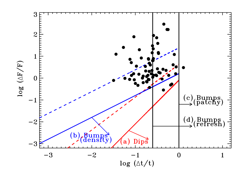
Figure 15: Scatter plot of $\Delta F/F$–$\Delta t/t$ values calculated on our flare samples on the kinematically allowed regions for afterglow variabilities according to Ioka et al. (2005). Data are drawn from Tables  2 and 3: we used the FWHM of the Gaussians as $\Delta t$, the Gaussian peak time for $t$, while the ratio of the peak flux over the underlying continuum flux ($\Delta F/F$) was calculated using the best fit models. The four limits plotted are based on (a) eq. (4) in Ioka et al. (2005) for dips (shown on axis), (b) eq. (7) for bumps due to density fluctuations (on axis), (c) $\Delta t>t$ for bumps due to patchy shells, and (d) $\Delta t>t/4$ for bumps due to refreshed shocks. According to Ioka et al. (2005), when many regions fluctuate simultaneously, limits a and b are replaced by eqs. (A1) and (A2) in Ioka et al. (2005), respectively. The off-axis cases (viewing angle $\theta_{v}\sim\gamma^{-1}/2\gtrsim\Delta\theta$, where $\Delta\theta\gtrsim\gamma^{-1}$ is the half-angular size of the variable region) are shown by dashed lines.

In light of the calculations of Ioka et al. (2005), we calculated $\Delta F/F$ and $\Delta t/t$ values from our flare sample and plotted them over the kinematically allowed regions for afterglow variabilities, as shown in Fig. 15. Ioka et al. (2005) distinguish between four cases: (a) dips, arising from non-uniformity on the emitting surface induced, e.g., by density fluctuations, [eq. (4) in Ioka et al. (2005)]; (b) bumps due to density fluctuations (Wang & Loeb, 2000; Lazzati et al., 2002; Dai & Lu, 2002) [eq. (7) in Ioka et al. (2005)]; (c) bumps due to patchy shells (Mészáros et al., 1998; Kumar & Piran, 2000a), for which $\Delta t>t$; (d) bumps due to refreshed shocks (Rees & Mészáros, 1998; Panaitescu et al., 1998; Kumar & Piran, 2000b), for which $\Delta t>t/4$.

Our findings are consistent with the conclusion of Zhang et al. (2006) and Lazzati & Perna (2007), the latter based on a preliminary presentation of our dataset in Chincarini (2006), i.e., a sizable fraction of the flares cannot be related to external shock mechanisms. In particular, only one point (corresponding to a flare in GRB 051117A) lies in the region of $\Delta t>t$, where flares are consistent with the patchy shells model; only three points (including the the early flare of GRB 050502B) lie in the region of flares that can be caused by ambient density fluctuations; finally, only 29/69 lie in the region that describes flares due to refreshed shocks. Among the rest, 10/69 can only be due to internal shocks.

Perna et al. (2006) proposed that X-ray flares are due to accretion of a fragmented disk. Due to viscous evolution, blobs far from the central black hole takes longer to be accreted and are therefore more spread-out when accretion occurs. The accretion rate is correspondingly lower. This naturally gives a peak luminosity-flare epoch anti-correlation as has been revealed by the data. This same merit could be retained if a magnetic barrier modulate a continuous accretion flow near the black hole at different epochs (Proga & Zhang, 2006).

Table 1: GRB XRT light curve sample.

GRB	Redshift	$T_{90}$	BAT Fluence	Reference	Reference	Notes
Name		(s)	(erg cm-2)	redshift	BAT
(1)	(2)	(3)	(4)	(5)	(6)	(7)
050406	$\cdots$	$5\pm 1$	$9.0\times 10^{-8}$	$\cdots$	1	XRF
050421	$\cdots$	$10.3\pm 2$	$(1.8\pm 0.7)\times 10^{-7}$	$\cdots$	2
050502B	$\cdots$	$17.5\pm 0.2$	$(8.0\pm 1.0)\times 10^{-7}$	$\cdots$	3
050607	$\cdots$	26.5	$(8.9\pm 1.2)\times 10^{-7}$	$\cdots$	4
050712	$\cdots$	$48\pm 2$	$1.8\times 10^{-6}$	$\cdots$	5
050713A	$\cdots$	$70\pm 10$	$(9.1\pm 0.6)\times 10^{-6}$	$\cdots$	6
050714B	$\cdots$	55.	$(6.5\pm 1.4)\times 10^{-7}$	$\cdots$	7	XRF
050716	$\cdots$	$69\pm 1$	$(8.3\pm 1.3)\times 10^{-6}$	$\cdots$	8
050724	0.258	$3\pm 1$	$(6.3\pm 1.0)\times 10^{-7}$	9	10	Short
050726	$\cdots$	30.	$(4.3\pm 0.7)\times 10^{-6}$	$\cdots$	11
050730	3.967	$155\pm 20$	$(4.4\pm 0.4)\times 10^{-6}$	12	13
050801	$\cdots$	$20\pm 3$	$(4.4\pm 1.0)\times 10^{-7}$	$\cdots$	14
050802	$\cdots$	$13\pm 2$	$(2.8\pm 0.3)\times 10^{-6}$	$\cdots$	15
050803	0.422	$85\pm 10$	$(3.9\pm 0.3)\times 10^{-6}$	16	17
050814	$\cdots$	$65^{+40}_{-20}$	$(2.17\pm 0.36)\times 10^{-6}$	$\cdots$	18
050819	$\cdots$	$36\pm 4$	$(4.2\pm 0.8)\times 10^{-7}$	$\cdots$	19
050820A	2.612	$26\pm 2$	$(1.9\pm 0.2)\times 10^{-6}$	20	21
050822	$\cdots$	$102\pm 2$	$(3.4\pm 0.3)\times 10^{-6}$	$\cdots$	22
050826	$\cdots$	$35\pm 8$	$(4.3\pm 0.7)\times 10^{-7}$	$\cdots$	23
050904	6.29	$225\pm 10$	$(5.4\pm 0.2)\times 10^{-6}$	24	25
050908	3.3437	$20\pm 2$	$(5.1\pm 0.5)\times 10^{-7}$	26	27
050915A	$\cdots$	$53\pm 3$	$(8.8\pm 0.9)\times 10^{-7}$	$\cdots$	28
050916	$\cdots$	$90\pm 10$	$(1.1\pm 0.4)\times 10^{-6}$	$\cdots$	29
050922B	$\cdots$	$80\pm 10$	$(1.8\pm 0.3)\times 10^{-6}$	$\cdots$	30
051016B	0.936	$4.0\pm 0.1$	$(1.7\pm 0.2)\times 10^{-7}$	31	32
051117A	$\cdots$	$140\pm 10$	$(4.6\pm 0.16)\times 10^{-6}$	$\cdots$	33
051210	$\cdots$	$1.4\pm 0.2$	$(8.3\pm 1.4)\times 10^{-8}$	$\cdots$	34	Short
051227	$\cdots$	$8.0\pm 0.2$	$(2.3\pm 0.3)\times 10^{-7}$	$\cdots$	35
060108	$\cdots$	$14.4\pm 1$	$(3.7\pm 0.4)\times 10^{-7}$	$\cdots$	36
060109	$\cdots$	$116\pm 3$	$(6.4\pm 1.0)\times 10^{-7}$	$\cdots$	37
060111A	$\cdots$	$13\pm 1$	$(1.18\pm 0.05)\times 10^{-6}$	$\cdots$	38
060115	3.53	$142\pm 5$	$(1.8\pm 0.2)\times 10^{-6}$	39	40
060124	2.296	$321\pm 2$	$(1.40\pm 0.03)\times 10^{-5}$	41	42

References. — (1) Krimm et al. (2005b); (2) Sakamoto et al. (2005a); (3) Cummings et al. (2005b); (4) Retter et al. (2005); (5) Markwardt et al. (2005a); (6) Palmer et al. (2005c); (7) Tueller et al. (2005a); (8) Barthelmy et al. (2005b); (9) Prochaska et al. (2005b); (10) Krimm et al. (2005a); (11) Barthelmy et al. (2005d); (12) Chen et al. (2005); (13) Markwardt et al. (2005c); (14) Sakamoto et al. (2005c); (15) Palmer et al. (2005a); (16) Bloom et al. (2005); (17) Parsons et al. (2005); (18) Tueller et al. (2005b); (19) Barthelmy et al. (2005c); (20) Prochaska et al. (2005a); (21) Cummings et al. (2005a); (22) Hullinger et al. (2005a); (23) Markwardt et al. (2005b); (24) Haislip et al. (2006); (25) Sakamoto et al. (2005b); (26) Fugazza et al. (2005); (27) Sato et al. (2005b); (28) Barthelmy et al. (2005a); (29) Fenimore et al. (2005); (30) Hullinger et al. (2005c); (31) Soderberg et al. (2005); (32) Barbier et al. (2005); (33) Palmer et al. (2005b); (34) Sato et al. (2005a); (35) Hullinger et al. (2005b); (36) Sakamoto et al. (2006); (37) Palmer et al. (2006); (38) Sato et al. (2006); (39) Piranomonte et al. (2006); (40) Barbier et al. (2006); (41) Mirabal & Halpern (2006); (42) Romano et al. (2006a).

Table 2: Fits to the XRT light curves: continuum parameters.

GRB	$\alpha_{1}$	$t_{\rm b1}$	$\alpha_{2}$	$t_{\rm b2}$	$\alpha_{3}$
		(s)		(s)
(1)	(2)	(3)	(4)	(5)	(6)
050406	$1.58_{-0.17}^{+0.17}$	$(4.36^{+6.23}_{-0.53})\times 10^{3}$	$0.50_{-0.14}^{+0.13}$	$\cdots$	$\cdots$
050421	$3.10_{-0.09}^{+0.11}$	$\cdots$	$\cdots$	$\cdots$	$\cdots$
050502B	$0.75_{-0.04}^{+0.04}$	$(15.2_{-4.3}^{+5.2})\times 10^{4}$	$1.77^{+0.32}_{-0.26}$	$\cdots$	$\cdots$
050607	$1.65_{-0.16}^{+0.17}$	$1.45\times 10^{3}\,\tablenotemark{b}$	$0.52^{+0.14}_{-0.16}$	$1.54\times 10^{4}\,\tablenotemark{b}$	$1.34^{+0.39}_{-0.26}$
050712	$2.17^{+0.38}_{-0.67}$	$3.44\times 10^{2}\,\tablenotemark{b}$	$3.12^{+0.37}_{-0.25}$	$8.39\times 10^{2}\,\tablenotemark{b}$	$0.43^{+0.27}_{-0.29}$
050713A	$7.16^{+0.84}_{-0.68}$	$1.12\times 10^{2}\,\tablenotemark{b}$	$0.81\,\tablenotemark{b}$	$\cdots$	$\cdots$
050714B	$6.79^{+0.35}_{-0.38}$	$(3.90_{-0.3}^{+0.31})\times 10^{2}$	$0.49^{+0.10}_{-0.09}$	$(8.03_{-7.80}^{+7.81})\times 10^{4}$	$0.79^{+0.33}_{-0.32}$
050716	$1.32^{+0.02}_{-0.07}$	$(4.70_{-0.15}^{+0.05})\times 10^{2}$	$8.8^{+1.40}_{-1.60}$	$\cdots$	$\cdots$
050724	$1.53^{+0.07}_{-0.07}$	$(1.90_{-0.04}^{+0.05})\times 10^{2}$	$5.8^{+0.50}_{-0.30}$	$(5.53_{-0.54}^{+0.60})\times 10^{2}$	$0.78_{-0.18}^{+0.13}$
050726	$0.95^{+0.04}_{-0.03}$	$(8.53_{-1.43}^{+1.32})\times 10^{3}$	$1.89^{+0.16}_{-0.20}$	$\cdots$	$\cdots$
050730	$0.28^{+0.04}_{-0.09}$	$(5.52_{-0.26}^{+0.34})\times 10^{3}$	$1.97^{+0.06}_{-0.04}$	$\cdots$	$\cdots$
050801	$0.57^{+0.22}_{-0.16}$	$(4.67_{-1.87}^{+1.90})\times 10^{2}$	$1.24^{+0.09}_{-0.08}$	$\cdots$	$\cdots$
050802	$0.27\,\tablenotemark{b}$	$(8.80_{-1.51}^{+2.10})\times 10^{3}$	$1.60^{+0.19}_{-0.25}$	$\cdots$	$\cdots$
050803	$4.54^{+0.26}_{-0.29}$	$(4.46_{-0.32}^{+0.33})\times 10^{2}$	$0.03^{+0.01}_{-0.08}$	$(1.27_{-0.58}^{+0.58})\times 10^{4}$	$1.59^{+0.03}_{-0.04}$
050814	$3.26^{+0.12}_{-0.20}$	$(9.99_{-0.98}^{+0.59})\times 10^{2}$	$0.56^{+0.09}_{-0.14}$	$(8.46_{-1.26}^{+1.24})\times 10^{4}$	$2.44^{+0.34}_{-0.46}$
050819	$3.22\,\tablenotemark{b}$	$(8.18\times 10^{2}\,\tablenotemark{b}$	$0.27\,\tablenotemark{b}$	$\cdots$	$\cdots$
050820A	$2.25^{+0.14}_{-0.17}$	$(2.00_{-0.19}^{+0.14})\times 10^{2}$	$0.03\,\tablenotemark{b}$	$(4.79_{-0.34}^{+0.52})\times 10^{3}$	$1.27^{+0.05}_{-0.06}$
050822	$2.99\,\tablenotemark{b}$	$7.50\times 10^{2}\,\tablenotemark{b}$	$0.40\,\tablenotemark{b}$	$(2.22\times 10^{4}\,\tablenotemark{b}$	$1.72\,\tablenotemark{b}$
050904	$1.57^{+0.12}_{-0.13}$	$(3.35_{-0.42}^{+0.40})\times 10^{2}$	$2.26^{+0.11}_{-0.10}$	$(1.70_{-0.36}^{+0.49})\times 10^{4}$	$0.50\,\tablenotemark{b}$
050908	$1.12^{+0.06}_{-0.06}$	$\cdots$	$\cdots$	$\cdots$	$\cdots$
050915A	$0.42^{+0.28}_{-0.27}$	$(1.74_{-0.71}^{+2.36})\times 10^{3}$	$1.20^{+0.20}_{-0.10}$	$\cdots$	$\cdots$
050916	$0.95^{+0.30}_{-0.25}$	$\cdots$	$\cdots$	$\cdots$	$\cdots$
050922B	$3.33^{+0.37}_{-0.30}$	$\cdots$	$\cdots$	$\cdots$	$\cdots$
051117A	$0.66^{+0.11}_{-0.10}$	$\cdots$	$\cdots$	$\cdots$	$\cdots$
051210	$2.58^{+0.25}_{-0.17}$	$\cdots$	$\cdots$	$\cdots$	$\cdots$
051227	$2.50^{+0.15}_{-0.15}$	$7.37\times 10^{2}\,\tablenotemark{b}$	$0.18\,\tablenotemark{b}$	$3.10\times 10^{3}\,\tablenotemark{b}$	$1.22\,\tablenotemark{b}$
060108	$2.60^{+0.55}_{-0.55}$	$(2.54_{-0.46}^{+0.45})\times 10^{2}$	$0.37^{+0.05}_{-0.05}$	$(1.87_{-0.36}^{+0.36})\times 10^{3}$	$1.22^{+0.09}_{-0.09}$
060111A	$-4.25_{-0.44}^{+0.36}$	$(3.25_{-0.37}^{+0.28})\times 10^{2}$	$6.26^{-0.27}_{+0.28}$	$(7.38_{-0.33}^{+0.37})\times 10^{2}$	$0.90_{-0.05}^{+0.05}$
060115	$3.29^{+0.21}_{-0.29}$	$(5.74_{-0.56}^{+0.86})\times 10^{2}$	$0.70^{+0.05}_{-0.08}$	$(3.91_{-1.37}^{+2.13})\times 10^{4}$	$1.31^{+0.22}_{-0.20}$
060124	$0.44_{-0.08}^{+0.07}$	$(1.0$–$11.5)\times 10^{3}$	$1.21\pm 0.04$	$(1.05_{-0.14}^{+0.17})\times 10^{5}$	$1.58\pm 0.06$

Table 3: Fits to the XRT flares: Gaussians, power-laws and exponentials.

GRB		Gaussian		$\Delta F/F$	EW	$\alpha_{\rm fall}$	$\tau_{90}$	$\Delta t_{\rm fall}/\Delta t_{\rm rise}$	$\Delta t/t$
	Center (s)	Width (s)	Norm (count s-1)		(s)		(s)
(1)	(2)	(3)	(4)	(5)	(6)	(7)	(8)	(9)	(10)
050406	$211_{-5}^{+5}$	$17.9_{-4.6}^{+12.3}$	$4.6_{-1.3}^{+1.2}$	$7.71$	686	$\cdots$	184.0	1.520	0.882
050421	$111_{-2}^{+0}$	$1.7_{-0.1}^{+0.1}$	$191.2_{-107.8}^{+1186.8}$	$12.35$	$\cdots$	$\cdots$	$\cdots$	$\cdots$	$\cdots$
	$154_{-3}^{+3}$	$6.2_{-4.1}^{+4.3}$	$4.7_{-1.9}^{+5.4}$	$0.84$	$\cdots$	$\cdots$	$\cdots$	$\cdots$	$\cdots$
050502B	$719_{-2}^{+1}$	$100.1_{-1.02}^{+1.2}$	$88.0_{-1.4}^{+1.3}$	$38.55$	127320	$6.3\pm 0.38$	523.6	1.450	1.352
	$33431_{-3391}^{+4057}$	$6273.0_{-2258}^{+2815}$	$0.012_{-0.005}^{+0.006}$	$0.28$	$\cdots$	$\cdots$	$\cdots$	$\cdots$	$\cdots$
	$74637_{-2581}^{+2429}$	$26742.9_{-2440.9}^{+2761.1}$	$0.027_{-0.003}^{+0.003}$	$1.57$	432630	$4.67\pm 0.34$	$\cdots$	$\cdots$	$\cdots$
050607	$330_{-7}^{+8}$	$36.1_{-5.4}^{+5.5}$	$15.8_{-3.1}^{+3.3}$	$21.84$	1813	$3.39\pm 0.24$	266.5	1.610	0.798
050712	$245.7_{-5.7}^{+3.3}$	$31.1_{-6.6}^{+5.0}$	$7.3_{-1.2}^{+1.2}$	$1.37$	$\cdots$	$\cdots$	$\cdots$	$\cdots$	$\cdots$
	$486.1_{-3.7}^{+4.9}$	$16.7_{-2.8}^{+4.1}$	$7.4_{-1.6}^{+1.5}$	$5.10$	165	$2.87\pm 0.41$	$\cdots$	$\cdots$	$\cdots$
	$913.5_{-21.1}^{+21.8}$	$98.9_{-15.7}^{+29.3}$	$1.0_{-0.27}^{+0.47}$	$6.35$	$\cdots$	$\cdots$	$\cdots$	$\cdots$	$\cdots$
050713A	$112.2_{-0.5}^{+0.6}$	$5.9_{-0.5}^{+0.5}$	$170.5_{-18.3}^{+17.6}$	$19.77$	190	$2.92\pm 0.25$	49.5	3.070	0.445
	$173.4_{-1.5}^{+1.6}$	$16.3_{-2.1}^{+2.0}$	$23.5_{-2.2}^{+2.4}$	$3.97$	94	$3.1\pm 0.2$	82.9	2.790	0.494
	$399.8_{-5.3}^{+9.9}$	$23.3_{-3.6}^{+5.1}$	$24.9_{-2.16}^{+3.4}$	$8.27$	$\cdots$	$\cdots$	$\cdots$	$\cdots$	$\cdots$
	$126.2_{-3.1}^{+3.8}$	$10.8_{-1.7}^{+1.3}$	$55.6_{-9.6}^{+11.5}$	$7.26$	$\cdots$	$\cdots$	$\cdots$	$\cdots$	$\cdots$
050714B	$399_{-8}^{+8}$	$52.4_{-6.1}^{+9.4}$	$4.4_{-0.9}^{+0.8}$	$69.86$	2313	$3.2\pm 0.43$	344.8	3.410	0.928
050716	$175_{-66}^{+0}$	$48_{-15}^{+19}$	$9.0_{-2}^{+14}$	$0.48$	240	$0.51\pm 0.24$	622.0	4.750	3.514
	$382_{-6}^{+5}$	$16.3_{-5.6}^{+7.2}$	$3.8_{-1.3}^{+1}$	$0.57$	383	$2.13\pm 0.51$	482.9	2.700	1.283
050724	$275_{-5}^{+5}$	$30.6_{-6}^{+6.6}$	$7.2_{-1.1}^{+1.1}$	$1.35$	84	$2.52\pm 0.5$	$\cdots$	$\cdots$	$\cdots$
	$327_{-9}^{+6}$	$12.7_{-5.0}^{+6.3}$	$3.1_{-1.0}^{+1.0}$	$1.58$	67	$4.43\pm 0.8$	$\cdots$	$\cdots$	$\cdots$
	$(5.7_{-0.3}^{+0.2})\times 10^{4}$	$(1.9_{-0.3}^{+0.3})\times 10^{4}$	$0.030_{-0.003}^{+0.004}$	$11.99$	737109	$3.13\pm 0.19$	112365	1.720	2.045
050726	$168_{-5}^{+5}$	$8.2_{-4.4}^{+6.7}$	$3.1_{-1.6}^{+1.9}$	$0.46$	8	$3.7\pm 1.2$	33.0	0.492	0.199
	$273_{-4}^{+4}$	$27.0_{-4.4}^{+5.1}$	$6.6_{-1}^{+1}$	$1.57$	126	$3.5\pm 0.53$	122.0	1.120	0.446
050730	$131.8_{-59.6}^{+12.7}$	$32.7_{-8.3}^{+24.4}$	$8.3_{-1.4}^{+9.2}$	$1.33$	$\cdots$	$\cdots$	$\cdots$	$\cdots$	$\cdots$
	$234.2_{-2.4}^{+2.7}$	$14.5_{-2.8}^{+3}$	$5.3_{-0.8}^{+0.9}$	$1.00$	43	$4.9\pm 1.1$	$\cdots$	$\cdots$	$\cdots$
	$436.5_{-2.2}^{+1.5}$	$38.5_{-2.5}^{+2.8}$	$9.0_{-0.5}^{+0.6}$	$2.02$	370	$\cdots$	$\cdots$	$\cdots$	$\cdots$
	$685.8_{-2.7}^{+2.8}$	$23.8_{-3.5}^{+3.9}$	$5.19_{-0.61}^{+0.69}$	$1.32$	224	$\cdots$	$\cdots$	$\cdots$	$\cdots$
	$742$	$10$	$3.0$	$0.78$	$\cdots$	$\cdots$	$\cdots$	$\cdots$	$\cdots$
	$4526.2_{-107.2}^{+112.8}$	$408.1_{-94.1}^{+126.9}$	$0.86_{-0.26}^{+0.24}$	$0.37$	350	$\cdots$	$\cdots$	$\cdots$	$\cdots$
	$10223.6_{-477.6}^{+203.4}$	$847_{-179}^{+3}$	$0.87_{-0.10}^{+0.12}$	$1.34$	1897	$\cdots$	$\cdots$	$\cdots$	$\cdots$
	$12182.9$	$383.2$	$0.4$	$0.87$	$\cdots$	$\cdots$	$\cdots$	$\cdots$	$\cdots$
050801	$284_{-35}^{+48}$	$49.5_{-42.5}^{+42.5}$	$1.0_{-0.7}^{+0.9}$	$0.91$	$\cdots$	$\cdots$	$\cdots$	$\cdots$	$\cdots$
050802	$464_{-31}^{+31}$	$100_{-40}^{+33}$	$2.14_{-0.74}^{+0.46}$	$2.25$	159	$2.54\pm 0.35$	926.3	5.300	2.327
050803	$332_{-19}^{+19}$	$29.0_{-22}^{+22}$	$0.8_{-0.5}^{+0.5}$	$0.85$	65	$1.7\pm 0.8$	$\cdots$	$\cdots$	$\cdots$
	$604$	$189.2$	$1.00$	$4.05$	357	$3.1\pm 1.2$	$\cdots$	$\cdots$	$\cdots$
	$1201$	$164.2$	$0.67$	$2.66$	404	$1.3\pm 3.2$	$\cdots$	$\cdots$	$\cdots$
050814	$2286_{-127}^{+769}$	$299.0_{-118.9}^{+423.7}$	$0.12_{-0.02}^{+0.02}$	$1.30$	$\cdots$	$\cdots$	$\cdots$	$\cdots$	$\cdots$
050819	$177_{-19}^{+7}$	$13.9_{-5.5}^{+11.72}$	$2.1_{-0.8}^{+1.0}$	$0.67$	8	$\cdots$	$\cdots$	$\cdots$	$\cdots$
050820A	$241_{-1}^{+0}$	$9.5_{-0.2}^{+0.3}$	$231.0_{-6.2}^{+6.2}$	$77.45$	$\cdots$	$\cdots$	$\cdots$	$\cdots$	$\cdots$
050822	$142.7_{-1.1}^{+1.2}$	$15.2_{-0.8}^{+1.0}$	$54.7_{-3.5}^{+3.7}$	$1.09$	59	$4.34\pm 0.17$	$\cdots$	$\cdots$	$\cdots$
	$241.8_{-1.6}^{+1.9}$	$12.4_{-1.7}^{+1.7}$	$15.5_{-2.1}^{+2.3}$	$1.50$	129	$2.78\pm 0.17$	110.3	1.280	0.459
	$465.7_{-1.6}^{+1.6}$	$49.0_{-0.4}^{+2.3}$	$43.5_{-1.46}^{+1.38}$	$29.89$	6851	$5.06\pm 0.18$	328.0	0.630	0.708
050904	$448.6_{-4}^{+3.7}$	$45.9_{-3.8}^{+4.5}$	$20.7_{-1.4}^{+1.2}$	$2.22$	401	$4.52\pm 0.32$	$\cdots$	$\cdots$	$\cdots$
	$975.5_{-32.5}^{+38.5}$	$62.8_{-32.5}^{+36.9}$	$1.0_{-0.2}^{+0.5}$	$0.62$	162	$\cdots$	$\cdots$	$\cdots$	$\cdots$
	$1265.5_{-27.0}^{+28.0}$	$81.6_{-28.2}^{+30.1}$	$1.1_{-0.3}^{+0.4}$	$1.23$	364	$\cdots$	$\cdots$	$\cdots$	$\cdots$
	$7112.8_{-102.8}^{+147.2}$	$790.4_{-81.6}^{+103.1}$	$1.6_{-0.1}^{+0.1}$	$88.46$	$\cdots$	$\cdots$	$\cdots$	$\cdots$	$\cdots$
	$16682.2_{-263.2}^{+260.8}$	$3194.8_{-227.8}^{+212.2}$	$0.77_{-0.04}^{+0.05}$	$292.29$	$\cdots$	$\cdots$	$\cdots$	$\cdots$	$\cdots$
	$31481.1_{-762.1}^{+724.9}$	$7149.6_{-647.6}^{+687.4}$	$0.31_{-0.02}^{+0.02}$	$166.67$	$\cdots$	$\cdots$	$\cdots$	$\cdots$	$\cdots$
050908	$146_{-18}^{+10}$	$23_{-23}^{+-23}$	$2.17_{-0.97}^{+0.93}$	$1.72$	88	$\cdots$	$\cdots$	$\cdots$	$\cdots$
	$425_{-11}^{+18}$	$45_{-15}^{+18}$	$2.4_{-0.7}^{+1.1}$	$6.29$	1132	$2.36\pm 0.11$	295.6	2.660	0.727
050915A	$107_{-5}^{+2}$	$15.5_{-2.6}^{+5.6}$	$12.20_{-1.5}^{+1.5}$	$13.36$	43	$3.35\pm 0.38$	$\cdots$	$\cdots$	$\cdots$
050916	$18750_{-105}^{+236}$	$425_{-105}^{+205}$	$0.2_{-0.1}^{+0.1}$	$25.22$	130717	$\cdots$	$\cdots$	$\cdots$	$\cdots$
	$21463_{-425}^{+696}$	$2222_{-360}^{+592}$	$0.1_{-0.03}^{+0.04}$	$14.34$	$\cdots$	$\cdots$	$\cdots$	$\cdots$	$\cdots$
050922B	$375_{-1}^{+2}$	$9.2_{-1.7}^{+2.1}$	$23.0_{-4}^{+3}$	$0.97$	221	$1.66\pm 0.33$	175.4	1.330	0.466
	$490_{-8}^{+8}$	$37.7_{-8}^{+9}$	$6.7_{-1.3}^{+1.1}$	$0.69$	410	$\cdots$	254.7	2.020	0.508
	$858_{-9}^{+10}$	$123_{-8}^{+9}$	$22.0_{-2}^{+2}$	$14.64$	14336	$6.76\pm 0.42$	464.9	1.420	0.572
051117A	$132_{-5}^{+5}$	$48_{-4}^{+4}$	$102_{-9}^{+6}$	$3.23$	27	$2.72\pm 0.46$	$331.9$	2.5	2.192
	$376_{-14}^{+18}$	$203_{-20}^{+14}$	$47_{-6}^{+4}$	$3.01$	195	$\cdots$	$\cdots$	$\cdots$	$\cdots$
	$955_{-6}^{+7}$	$69_{-5}^{+6}$	$29_{-2}^{+1}$	$3.41$	395	$3.51\pm 0.28$	$\cdots$	$\cdots$	$\cdots$
	$1110_{-5}^{+5}$	$50_{-4}^{+4}$	$27_{-2}^{+2}$	$3.51$	1201	$\cdots$	$\cdots$	$\cdots$	$\cdots$
	$1341_{-2}^{+3}$	$43_{-2}^{+3}$	$49_{-2}^{+3}$	$7.21$	$\cdots$	$\cdots$	603.4	8.060	0.453
	$1516_{-7}^{+9}$	$135_{-9}^{+7}$	$30_{-1.3}^{+1.2}$	$4.78$	$\cdots$	$6.6\pm 4.0$	$\cdots$	$\cdots$	$\cdots$
051210	$134.4_{-4.4}^{+3.6}$	$10.4_{-4.1}^{+5.7}$	$4.7_{-1.7}^{+1.7}$	$1.18$	16	$4.05\pm 0.57$	49.2	0.490	0.360
	$216.2$	$63.1$	$0.62$	$0.53$	$\cdots$	$\cdots$	$\cdots$	$\cdots$	$\cdots$
051227	$124.2$	$10.5$	$5.15$	$0.88$	$\cdots$	$2.05\pm 0.5$	$\cdots$	$\cdots$	$\cdots$
060108	$303.5_{-24.5}^{+23.5}$	$44.5_{-30.5}^{+125.5}$	$0.3_{-0.12}^{+0.18}$	$1.83$	25		$\cdots$	$\cdots$	$\cdots$
060111A	$95.1_{-1.5}^{+1.4}$	$22.8_{-1.7}^{+2.1}$	$67.6_{-2.8}^{+2.7}$	$165.51$	73	$3.53\pm 0.39$	144.4	0.800	1.405
	$166.9_{-1.6}^{+1.6}$	$18.4_{-1.8}^{+2.0}$	$34.7_{-2.2}^{+2.1}$	$7.78$	54	$4.5\pm 1.2$	120.7	1.230	0.719
	$280.1_{-1.5}^{+1.3}$	$20.6_{-1.79}^{+1.73}$	$85.0_{-5.24}^{+4.59}$	$2.11$	931	$6.51\pm 0.4$	177.5	2.430	0.620
060115	$431.9_{-18.5}^{+18.5}$	$79.1_{-23.5}^{+25.8}$	$1.91_{-0.45}^{+0.54}$	$2.53$	144.2	$\cdots$	$\cdots$	$\cdots$	$\cdots$

Table 4: Properties of the 46 gamma-ray pulses detected from the BAT light curves of 28 GRBs with X-ray flares.

GRB	N	Bin	Peak	Peak	Error on Peak
Name		T (s)	Time (s)	Rate (counts s-1)	Rate (counts s-1)
(1)	(2)	(3)	(4)	(5)	(6)
050406	1	2.176	2.24	0.04144	0.00546
050421	1	10.688	11.072	0.01538	0.00256
050502B	1	0.384	0.864	0.23168	0.01581
050607	1	1.216	1.656	0.12026	0.00919
	2	13.952	16.888	0.03721	0.00256
050712	1	30.464	26.912	0.03095	0.00237
050713A	1	5.312	$-$54.89	0.04249	0.00675
	2	1.664	2.712	0.53963	0.01724
	3	6.400	10.84	0.40561	0.00926
	4	3.520	69.4	0.05585	0.00542
	5	12.032	116.70	0.01849	0.00233
050714B	1	23.68	52.392	0.02617	0.00313
050716	1	4.288	11.81	0.22210	0.01168
	2	11.648	46.94	0.12358	0.00648
050724	1	0.128	0.104	1.29947	0.07964
	2	0.064	210.92	0.29937	0.04221
050726	1	2.368	$-$173.87	0.09576	0.01595
	2	7.104	7.89	0.10490	0.00968
050730	1	13.824	17.432	0.04678	0.00286
050801	1	0.512	0.592	0.20882	0.01472
050802	1	12.736	13.90	0.02504	0.00256
050803	1	1.600	1.168	0.32463	0.02357
050814	1	16.512	18.856	0.04661	0.00450
050819	1	16.128	23.224	0.02246	0.00231
050822	1	3.264	3.912	0.15719	0.01272
	2	0.96	48.52	0.24216	0.01586
	3	4.352	60.04	0.10462	0.00577
	4	2.624	103.56	0.04600	0.00684
050904	1	6.976	29.768	0.06191	0.00493
	2	15.808	125.128	0.05769	0.00229
050908	1	3.072	3.776	0.07615	0.00586
050915A	1	5.376	5.496	0.05597	0.00436
	2	0.768	14.584	0.11584	0.01225
	3	1.920	44.6	0.03813	0.00520
050916	1	16.448	51.304	0.03522	0.00376
050922B	1	15.168	52.072	0.06915	0.00699
	2	14.336	103.4	0.05754	0.00705
	3	1.408	263.464	0.06536	0.00757
	4	1.216	271.656	0.06913	0.00825
051117A	1	8.704	11.264	0.08273	0.00388
051210	1	0.640	0.88	0.1057	0.01215
051227	1	0.640	0.80	0.12975	0.01213
060108	1	2.56	3.304	0.08358	0.00554
060111A	1	2.816	5.792	0.19368	0.00639
060115	1	5.312	6.352	0.05227	0.00438
	2	3.52	98.192	0.09428	0.00513

Table 5: Frequency distribution of the number of BAT pulses vs. the number of X-ray flares in 28 bursts.

Number of BAT Pulses	Numer of X-ray flares	Frequency
(1)	(2)	(3)
1	1	8
1	2	4
1	3	4
1	6	1
1	8	1
2	1	2
2	2	2
2	3	1
2	6	1
3	1	1
4	3	2
5	4	1

Table 6: Central times of the $\gamma$-ray pulses and X-ray flares for each GRB.

GRB	BAT	XRT					Times
Name	$n_{\gamma}$	$n_{\rm x}$	(s)	(s)	(s)	(s)	(s)	(s)	(s)	(s)	(s)
(1)	(2)	(3)	(4)	(5)	(6)	(7)	(8)	(9)	(10)	(11)	(12)
050406	1	1	2.24	211.0	$\cdots$	$\cdots$	$\cdots$	$\cdots$	$\cdots$	$\cdots$	$\cdots$
050421	1	2	11.072	111.0	154.0	$\cdots$	$\cdots$	$\cdots$	$\cdots$	$\cdots$	$\cdots$
050502B	1	3	0.864	719.0	33431.	74637.	$\cdots$	$\cdots$	$\cdots$	$\cdots$	$\cdots$
050607	2	1	1.656	16.888	330.0	$\cdots$	$\cdots$	$\cdots$	$\cdots$	$\cdots$	$\cdots$
050712	1	3	26.912	245.7	486.1	913.5	$\cdots$	$\cdots$	$\cdots$	$\cdots$	$\cdots$
050713A	5	4	$-$54.89	2.712	10.84	69.4	116.70	112.2	126.2	173.4	399.8
050714B	1	1	52.392	399.0	$\cdots$	$\cdots$	$\cdots$	$\cdots$	$\cdots$	$\cdots$	$\cdots$
050716	2	2	11.81	46.94	175.0	382.0	$\cdots$	$\cdots$	$\cdots$	$\cdots$	$\cdots$
050724	2	3	0.104	210.92	275.0	327.0	57000.0	$\cdots$	$\cdots$	$\cdots$	$\cdots$
050726	2	2	$-$173.87	7.89	168.0	273.0	$\cdots$	$\cdots$	$\cdots$	$\cdots$
050730	1	8	17.432	131.	234.2	436.5	685.8	742.0	4526.2	10223.6	12182.9
050801	1	1	0.592	284.0	$\cdots$	$\cdots$	$\cdots$	$\cdots$	$\cdots$	$\cdots$	$\cdots$
050802	1	1	13.90	464.0	$\cdots$	$\cdots$	$\cdots$	$\cdots$	$\cdots$	$\cdots$	$\cdots$
050803	1	3	1.168	332.0	604.0	1201.0	$\cdots$	$\cdots$	$\cdots$	$\cdots$	$\cdots$
050814	1	1	18.856	2286.0	$\cdots$	$\cdots$	$\cdots$	$\cdots$	$\cdots$	$\cdots$	$\cdots$
050819	1	1	23.224	177.0	$\cdots$	$\cdots$	$\cdots$	$\cdots$	$\cdots$	$\cdots$	$\cdots$
050822	4	3	3.912	48.52	60.04	103.56	142.7	241.8	465.7	$\cdots$	$\cdots$
050904	2	6	29.768	125.128	448.6	975.5	1265.5	7112.8	16682.2	31481.1	$\cdots$
050908	1	2	3.776	146.0	425.0	$\cdots$	$\cdots$	$\cdots$	$\cdots$	$\cdots$	$\cdots$
050915A	3	1	5.496	14.584	44.6	107.0	$\cdots$	$\cdots$	$\cdots$	$\cdots$	$\cdots$
050916	1	2	51.304	18750.0	21463.0	$\cdots$	$\cdots$	$\cdots$	$\cdots$	$\cdots$	$\cdots$
050922B	4	3	52.072	103.4	263.464	271.656	375.0	490.0	858.0	$\cdots$	$\cdots$
051117A	1	6	11.264	131.7	375.9	955.0	1110.0	1341.0	1516.0	$\cdots$	$\cdots$
051210	1	2	0.88	134.4	216.2	$\cdots$	$\cdots$	$\cdots$	$\cdots$	$\cdots$	$\cdots$
051227	1	1	0.80	124.2	$\cdots$	$\cdots$	$\cdots$	$\cdots$	$\cdots$	$\cdots$	$\cdots$
060108	1	1	3.304	303.5	$\cdots$	$\cdots$	$\cdots$	$\cdots$	$\cdots$	$\cdots$	$\cdots$
060111A	1	3	5.792	95.1	166.9	280.1	$\cdots$	$\cdots$	$\cdots$	$\cdots$	$\cdots$
060115	2	1	6.352	98.192	431.9	$\cdots$	$\cdots$	$\cdots$	$\cdots$	$\cdots$	$\cdots$

Figure 9: The results of the simulation in the $(t,\Delta t)$ plane: here we plot the contours for which we have the same detection probability. Black points are the real data, based on Gaussian widths and peaks. The dashed lines correspond to the three levels $\Delta t=1$, 0.1, and $2\times 10^{-3}$.

Figure 10: Ratio between the peaks of two successive events for both classes: X-ray flares (crosses) and gamma-ray pulses (circles), as a function of the quiescent time between the two events. Solid line shows the mean value, $-0.157$, when the two points with the lowest ratio are ignored; dashed lines show the $\pm 1\sigma$ region. The outliers are GRB 050724 ($\log{\rm peak}_{i+i}/{\rm peak}_{i}\sim 10^{-2}$) and GRB 050502B ($\log{\rm peak}_{i+i}/{\rm peak}_{i}\sim 10^{-4}$).

Figure 13: $EW/t_{\rm peak}$ vs. $\Delta t/t_{\rm peak}$. The solid line is the bisector of the plane.

Figure 14: $\Delta t_{\rm fall}/\Delta t_{\rm rise}$ vs $\tau_{90}$.

References

- Band et al. (1993) Band, D. et al. 1993, ApJ, 413, 281
- Barbier et al. (2006) Barbier, L. et al. 2006, GCN Circ., 4518, 1
- Barbier et al. (2005) —. 2005, GCN Circ., 4104, 1
- Barthelmy et al. (2005a) Barthelmy, S. et al. 2005a, GCN Circ., 3982, 1
- Barthelmy et al. (2005b) —. 2005b, GCN Circ., 3629, 1
- Barthelmy et al. (2005c) —. 2005c, GCN Circ., 3828, 1
- Barthelmy et al. (2005d) —. 2005d, GCN Circ., 3682, 1
- Barthelmy et al. (2005e) Barthelmy, S. D. et al. 2005e, Space Science Review, 120, 143
- Barthelmy et al. (2005f) —. 2005f, Nature, 438, 994
- Bloom et al. (2005) Bloom, J. S., Perley, D., Foley, R., Prochaska, J. X., Chen, H. W., & Starr, D. 2005, GCN Circ., 3758, 1
- Burrows et al. (2005a) Burrows, D. N. et al. 2005a, Space Science Review, 120, 165
- Burrows et al. (2005b) —. 2005b, Science, 309, 1833
- Burrows et al. (2006) Burrows, D. N. et al. 2006, in ESA SP-604: The X-ray Universe 2005, ed. A. Wilson, 877
- Campana et al. (2006) Campana, S. et al. 2006, A&A, 454, 113
- Chen et al. (2005) Chen, H.-W., Thompson, I., Prochaska, J. X., & Bloom, J. 2005, GCN Circ., 3709, 1
- Chincarini (2006) Chincarini, G. 2006, in Procs. of the Vulcano Workshop 2006, Vulcano, Italy, May 22–27, ed. F. Giovannelli & G. Mannocchi, astro–ph/0608414
- Chincarini et al. (2006) Chincarini, G. et al. 2006, in ESA SP-604: The X-ray Universe 2005, ed. A. Wilson, 871
- Chincarini et al. (2005) Chincarini, G. et al. 2005, arXiv:astro-ph/0506453
- Cummings et al. (2005a) Cummings, J. et al. 2005a, GCN Circ., 3835, 1
- Cummings et al. (2005b) —. 2005b, GCN Circ., 3339, 1
- Cusumano et al. (2006) Cusumano, G. et al. 2006, Nature, 440, 164
- Dai & Lu (2002) Dai, Z. G., & Lu, T. 2002, ApJ, 565, L87
- Daigne & Mochkovitch (1998) Daigne, F., & Mochkovitch, R. 1998, MNRAS, 296, 275
- Dermer (2004) Dermer, C. D. 2004, ApJ, 614, 284
- Eichler & Granot (2006) Eichler, D., & Granot, J. 2006, ApJ, 641, L5
- Falcone et al. (2006) Falcone, A. D. et al. 2006, ApJ, 641, 1010
- Falcone et al. (2007) —. 2007, ApJ, submitted
- Fenimore et al. (2005) Fenimore, E. et al. 2005, GCN Circ., 4003, 1
- Ford et al. (1995) Ford, L. A. et al. 1995, ApJ, 439, 307
- Fugazza et al. (2005) Fugazza, D. et al. 2005, GCN Circ., 3948, 1
- Gehrels et al. (2004) Gehrels, N. et al. 2004, ApJ, 611, 1005
- Gehrels et al. (2006) —. 2006, Nature, in pres, ArXiv Astrophysics e-prints, astro-ph/0610635
- Goad et al. (2006) Goad, M. R. et al. 2006, A&A, 449, 89
- Haislip et al. (2006) Haislip, J. B. et al. 2006, Nature, 440, 181
- Heise et al. (2001) Heise, J., in’t Zand, J., Kippen, R. M., & Woods, P. M. 2001, in Gamma-ray Bursts in the Afterglow Era, ed. E. Costa, F. Frontera, & J. Hjorth, 16–+
- Hill et al. (2004) Hill, J. E. et al. 2004, in X-Ray and Gamma-Ray Instrumentation for Astronomy XIII. Edited by Flanagan, Kathryn A.; Siegmund, Oswald H. W. Proceedings of the SPIE, Volume 5165, pp. 217-231 (2004)., ed. K. A. Flanagan & O. H. W. Siegmund, 217–231
- Hullinger et al. (2005a) Hullinger, D. et al. 2005a, GCN Circ., 3856, 1
- Hullinger et al. (2005b) —. 2005b, GCN Circ., 4400, 1
- Hullinger et al. (2005c) —. 2005c, GCN Circ., 4019, 1
- Ioka et al. (2005) Ioka, K., Kobayashi, S., & Zhang, B. 2005, ApJ, 631, 429
- Kobayashi et al. (2007) Kobayashi, S., Zhang, B., Mészáros, P., & Burrows, D. 2007, ApJ, 655, 391
- Krimm et al. (2005a) Krimm, H. et al. 2005a, GCN Circ., 3667, 1
- Krimm et al. (2005b) —. 2005b, GCN Circ., 3183, 1
- Kumar & Panaitescu (2000) Kumar, P., & Panaitescu, A. 2000, ApJ, 541, L51
- Kumar & Piran (2000a) Kumar, P., & Piran, T. 2000a, ApJ, 535, 152
- Kumar & Piran (2000b) —. 2000b, ApJ, 532, 286
- Lazzati & Perna (2007) Lazzati, D., & Perna, R. 2007, MNRAS, in press, astro-ph/0610730
- Lazzati et al. (2002) Lazzati, D., Rossi, E., Covino, S., Ghisellini, G., & Malesani, D. 2002, A&A, 396, L5
- Li & Fenimore (1996) Li, H., & Fenimore, E. E. 1996, ApJ, 469, L115
- Liang et al. (2006) Liang, E. W. et al. 2006, ApJ, 646, 351
- Markwardt et al. (2005a) Markwardt, C. et al. 2005a, GCN Circ., 3576, 1
- Markwardt et al. (2005b) —. 2005b, GCN Circ., 3888, 1
- Markwardt et al. (2005c) Markwardt, C. B. et al. 2005c, GCN Circ., 3715, 1
- Mészáros et al. (1998) Mészáros, P., Rees, M. J., & Wijers, R. A. M. J. 1998, ApJ, 499, 301
- Mirabal & Halpern (2006) Mirabal, N., & Halpern, J. P. 2006, GCN Circ., 4591, 1
- Norris et al. (1996) Norris, J. P., Nemiroff, R. J., Bonnell, J. T., Scargle, J. D., Kouveliotou, C., Paciesas, W. S., Meegan, C. A., & Fishman, G. J. 1996, ApJ, 459, 393
- Nousek et al. (2006) Nousek, J. A. et al. 2006, ApJ, 642, 389
- O’Brien et al. (2006) O’Brien, P. T. et al. 2006, ApJ, 647, 1213
- Pagani et al. (2006) Pagani, C. et al. 2006, ApJ, 645, 1315
- Palmer et al. (2006) Palmer, D. et al. 2006, GCN Circ., 4476, 1
- Palmer et al. (2005a) —. 2005a, GCN Circ., 3737, 1
- Palmer et al. (2005b) —. 2005b, GCN Circ., 4289, 1
- Palmer et al. (2005c) —. 2005c, GCN Circ., 3597, 1
- Panaitescu & Kumar (2000) Panaitescu, A., & Kumar, P. 2000, ApJ, 543, 66
- Panaitescu et al. (1998) Panaitescu, A., Mészáros, P., & Rees, M. J. 1998, ApJ, 503, 314
- Parsons et al. (2005) Parsons, A. et al. 2005, GCN Circ., 3757, 1
- Perna et al. (2006) Perna, R., Armitage, P. J., & Zhang, B. 2006, ApJ, 636, L29
- Piranomonte et al. (2006) Piranomonte, S. et al. 2006, GCN Circ., 4520, 1
- Piro et al. (1999) Piro, L. et al. 1999, ApJ, 514, L73
- Piro et al. (2005) —. 2005, ApJ, 623, 314
- Prochaska et al. (2005a) Prochaska, J. X., Bloom, J. S., Wright, J. T., Butler, R. P., Chen, H. W., Vogt, S. S., & Marcy, G. W. 2005a, GCN Circ., 3833, 1
- Prochaska et al. (2005b) Prochaska, J. X., Chen, H.-W., Bloom, J. S., & Stephens, A. 2005b, GCN Circ., 3679, 1
- Proga & Zhang (2006) Proga, D., & Zhang, B. 2006, MNRAS, 370, L61
- Rees & Mészáros (1998) Rees, M. J., & Mészáros, P. 1998, ApJ, 496, L1+
- Retter et al. (2005) Retter, A. et al. 2005, GCN Circ., 3525, 1
- Romano et al. (2006a) Romano, P. et al. 2006a, A&A, 456, 917
- Romano et al. (2006b) —. 2006b, A&A, 450, 59
- Sakamoto et al. (2006) Sakamoto, T. et al. 2006, GCN Circ., 4445, 1
- Sakamoto et al. (2005a) —. 2005a, GCN Circ., 3305, 1
- Sakamoto et al. (2005b) —. 2005b, GCN Circ., 3938, 1
- Sakamoto et al. (2005c) —. 2005c, GCN Circ., 3730, 1
- Sato et al. (2005a) Sato, G. et al. 2005a, GCN Circ., 4318, 1
- Sato et al. (2005b) —. 2005b, GCN Circ., 3951, 1
- Sato et al. (2006) —. 2006, GCN Circ., 4486, 1
- Soderberg et al. (2005) Soderberg, A. M., Berger, E., & Ofek, E. 2005, GCN Circ., 4186, 1
- Tagliaferri et al. (2005) Tagliaferri, G. et al. 2005, Nature, 436, 985
- Tueller et al. (2005a) Tueller, J. et al. 2005a, GCN Circ., 3615, 1
- Tueller et al. (2005b) —. 2005b, GCN Circ., 3803, 1
- Vaughan et al. (2006) Vaughan, S. et al. 2006, ApJ, 638, 920
- Wang & Loeb (2000) Wang, X., & Loeb, A. 2000, ApJ, 535, 788
- Willingale et al. (2007) Willingale, R. et al. 2007, ApJ, submitted, ArXiv Astrophysics e-prints, astro-ph/0612031
- Wu et al. (2005) Wu, X. F., Dai, Z. G., Wang, X. Y., Huang, Y. F., Feng, L. L., & Lu, T. 2005, ApJ, submitted, ArXiv Astrophysics e-prints, astro-ph/0512555
- Zhang et al. (2006) Zhang, B., Fan, Y. Z., Dyks, J., Kobayashi, S., Mészáros, P., Burrows, D. N., Nousek, J. A., & Gehrels, N. 2006, ApJ, 642, 354