On the origin of GeV photons in gamma-ray burst afterglows
Abstract
Fermi/LAT has detected long-lasting high-energy photons () from gamma-ray bursts (GRBs), with the highest energy photons reaching about 100 GeV. One proposed scenario is that they are produced by high-energy electrons accelerated in GRB forward shocks via synchrotron radiation. We study the maximum synchrotron photon energy in this scenario, considering the properties of the microturbluence magnetic fields behind the shock, as revealed by recent Particle-in-Cell simulations and theoretical analyses of relativistic collisionless shocks. Due to the small-scale nature of the micro-turbulent magnetic field, the Bohm acceleration approximation, in which the scattering mean free path is equal to the particle Larmor radius, breaks down at such high energies. This effect leads to a typical maximum synchrotron photon of a few GeV at 100 s after the burst and this maximum synchrotron photon energy decreases quickly with time. We show that the fast decrease of the maximum synchrotron photon energy leads to a fast decay of the synchrotron flux. The 10-100 GeV photons detected after the prompt phase can not be produced by the synchrotron mechanism. They could originate from the synchrotron self-Compton emission of the early afterglow if the circum-burst density is sufficiently large, or from the external inverse-Compton process in the presence of central X-ray emission, such as X-ray flares and prompt high-latitude X-ray emission.
1 Introduction
The Fermi satellite has opened a new window at high energies in studying gamma-ray bursts (GRBs). So far, Fermi large area telescope (LAT) has detected high-energy photons above 100 MeV from more than 40 GRBs (Ackermann et al. 2013). The high-energy emission (100 MeV) generally lasts much longer than the prompt KeV/MeV emission. The widely discussed scenario for this extended GeV emission is the external shock model, where electrons are accelerated by external forward shocks and produce GeV photons via synchrotron radiation (Kumar & Barniol Duran 2009, 2010; Ghisellini et al. 2009; Wang et al. 2010). The highest energy of these photons reached about 100 GeV (in the local redshift frame) during the early afterglows, as have been seen in GRB 090902B, GRB 090926A, and GRB 130427A (Abdo et al. 2009a;2009b; 2011a; Zhu et al. 2013). This posed a challenge for the external shock synchrotron scenario since the maximum synchrotron photon energy for accelerated electrons under the most favorable condition (i.e. the Bohm acceleration) is about 50 MeV in the shock rest frame111Kumar et al. (2012) suggest that particles can be accelerated in the low background magnetic field region and radiate in the high magnetic field region (i.e. in the amplified turbulence magnetic field region), so the maximum synchrotron emission can exceed 50 MeV. However, once the particles enter into the low background magnetic field region, the particles can not be scattered back to the upstream due to the lack of micro-turbulence, and the acceleration will not continue. and the bulk Lorentz factor of the external shock is at s after the burst trigger (Piran & Nakar 2010; Barniol Duran & Kumar 2011; Sagi & Nakar 2012). The maximum synchrotron photon energy 50 MeV is obtained in the assumption of the fastest acceleration – the Bohm acceleration, where the acceleration time is equal to the Larmor time of the particles in the magnetic field (i.e. by equating the Larmor time with the synchrotron cooling time in the magnetic field).
GRB afterglows are produced by relativistic collisionless shocks expanding into a weakly magnetized ambient medium. In such shocks, it is expected that the beam of super-thermal particles excite micro-turbulence on plasma scales in the ambient medium (Medvedev & Loeb 1999), where is the plasma frequency. The Particle-in-Cell (PIC) simulations indicate that the turbulence magnetic field quickly relaxes behind the shock transition to a sub-equipartition value of on spatial scales of (Chang et al. 2008; Keshet et al. 2009). Such microturbulence is expected to decay (Gruzinov & Waxman 1999) on larger scales; these recent simulations characterize the decay by a power law (where is the distance from the shock front and is the decay length of the magnetic field downstream from the shock). Modelling of the broad band emission of LAT GRBs indeed points to the decay of the magnetic field downstream of the shock, with , see Lemoine (2013) and Lemoine et al. (2013).
In relativistic collionless shocks responsible for the GRB afterglows, the Bohm approximation may not be valid for maximum energy electrons due to the small-scale nature of the micro-turbulence generated in the shock layer (Kirk & Reville 2009; Plotnikov et al. 2013; Lemoine 2013; Sironi et al. 2013), i.e. the Larmor radius of the maximum energy electrons is much larger than the length of the magnetic field, resulting a longer time for electrons finishing a scattering cycle. The maximum electron energy thus decreases, leading to a maximum synchrotron photon energy significantly smaller than 50 MeV in the shock rest frame and thus posing even more severe challenge for the synchrotron scenario. The typical maximum synchrotron photon energy, as shown in §2, is around GeV energies at hundreds of seconds after the burst and this maximum energy decreases quickly with time. We will show, in §3, that the decreasing maximum photon energy could lead to a fast decay of the synchrotron high-energy afterglow.
10-100 GeV photons detected after the prompt phase have energies exceeding the maximum synchrotron photon energy, and thus must have another origin. In §4, we study whether these highest energy photons can be produced by the inverse Compton (IC) emission in the afterglow, including the synchrotron self-Compton emission from the afterglow and the external IC emission of central X-ray emission. Finally we give our discussions and conclusions in §5.
2 The maximum synchrotron photon energy
The acceleration of particles in GRB forward shocks is believed to be governed by the Fermi mechanism. A non-thermal power-law spectrum is formed, described by , where is the electron Lorentz factor. Because the Lamor radius for maximum energy electrons, as shown below, particles only suffer a random small angle deflection of the order of as they cross a coherence cell of size . Therefore, the Bohm approximation breaks down and the residence time scale downstream is given by , where is the number of scatterings that the electrons experience before returning to the upstream and is the time spent in crossing the coherence cell.
By equating the synchrotron cooling time with the residence time , where is the magnetic field in the downstream region, we obtain the Lorentz factor of the maximal energy electrons (Kirk & Reville 2009, Plotnikov et al. 2013; Sironi et al. 2013) , i.e.
| (1) |
where and is the number density of the surrounding interstellar medium. Note that this Lorentz factor is independent of the magnetic field.
Since higher energy electrons travel a shorter distance before losing their energy, they radiate their energy at the place closer to the shock front. Thus, one expects that the highest energy synchrotron photons are emitted by the highest energy electrons at the place in very close proximity to the shock front, while the low-frequency emission with , which are produced by electrons with Lorentz factor whose cooling timescale is longer than the dynamic timescale, are emitted at the back of the shock. As the microturbulence magnetic field decays with the distance from the shock front, we assume for the high-energy emission detected by Fermi/LAT, while assume a value for low-energy afterglows, where could be much smaller than (see Lemoine 2013, Lemoine et al. 2013 for details).
One can check that the Bohm approximation for fails at this maximal Lorentz factor because
| (2) |
Assuming a constant parameter, one can derive the time evolution of the maximum synchrotron photon energy from Eq. (1). For a constant external density, one derives (see also Sironi et al. 2013)
| (3) |
For the wind case, (Sironi et al. 2013) . In this Letter, we assume that the circumburst medium has a constant density, but the result in section 3 holds also for the wind case.
3 Light curves of the MeV emission
Since decreases quickly with time (), the synchrotron flux in the LAT energy window (i.e. MeV) may decay faster than expected when approaches to the low threshold energy of the LAT window (i.e. 100 MeV). For a spectrum of , the integrated flux from the LAT threshold energy to the maximum energy is given by
| (4) |
where is the decay slope of the high-energy emission if is infinity, which is typically for high-energy gamma-ray emission.
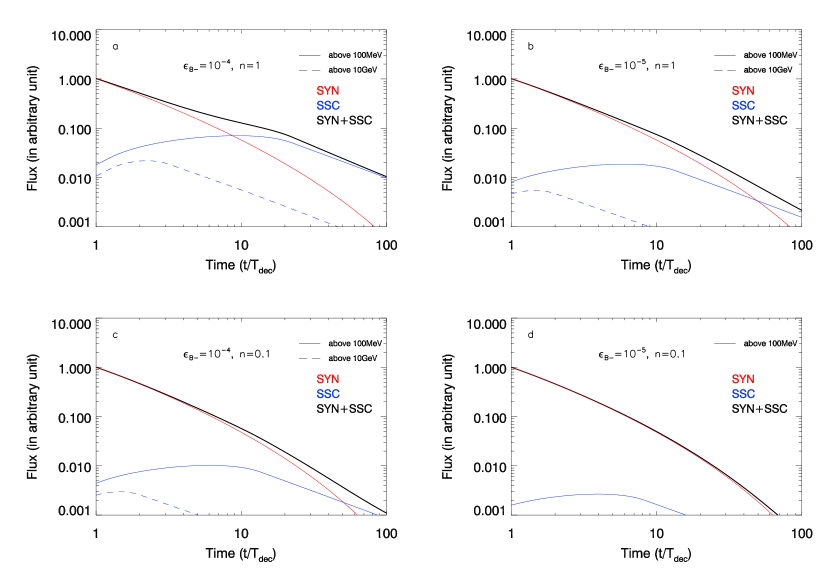
We show in Fig.1 some examples of the light curve of the synchrotron flux. We also calculate the self-synchrotron Compton (SSC) component contribution to the flux above 100 MeV. As can be seen from Fig.1, the relative strength between the synchrotron component and the SSC component can lead to different shapes of the observed light curves. In Fig. 1(a) and (b), the two components add together to form a late flattening or an almost straight power-law, even though the synchrotron component decays quickly at a few tens of the deceleration time. When the density of the circumburst medium is lower, the SSC component is not important even at late times. In this case, we will see an increasingly decaying synchrotron light curves, as described by Fig.1(c) and Fig. 1(d).
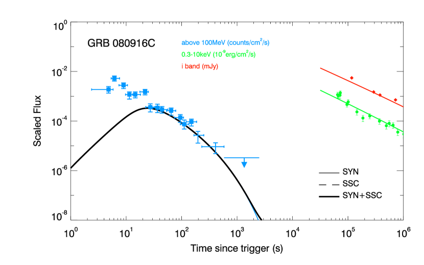
As an example, we fit the broad-band light curves of GRB 080916C. The LAT emission above 100 MeV decays quickly with a slope of (Ackermann et al. 2013), which is much faster than the expected from the standard synchrotron afterglow scenario. By invoking the effect of the decreasing maximum photon energy, we can reproduce such a fast decay, as shown in Fig.2. Note that the high-energy emission before s should be attributed to the prompt emission. A radiative blast wave interpretation for the fast decay has also been proposed by Ghisellini et al. (2010). This scenario needs a high value of the electron equipartition factor (i.e., ) in addition to a fast-cooling electron spectrum.
4 Inverse Compton origin for the 10-100 GeV photons
As we have shown, the synchrotron photon energy is limited to be a few GeV at seconds after the burst, so the 10-100 GeV photons detected during the afterglow phase must have another origin. Inverse-Compton mechanism is then the most natural mechanism. During the afterglow phase, there are two main sources of the IC emission, one is the SSC emission of the forward shock electrons and another is the external IC of central X-ray emission, such as X-ray flares and prompt high-latitude X-ray emission, by the forward shock electrons. Here we first study whether the SSC mechanism can explain these highest photons. Such scenario has been discussed in Zhang & Mészáros (2001) for high-energy emission before the Fermi era.
4.1 Synchrotron self-Compton mechanism
In the SSC scenario, the highest energy photons are mainly produced by electrons with energy scattering off afterglow photons, so we should use the magnetic field in the back of the shock in the calculation (i.e. ). The value of is found to be from the broad-band fitting of the LAT GRB data (e.g. Kumar & Barniol Duran 2010; Liu & Wang 2011; He et al. 2011; Lemoine et al. 2013). The cooling Lorentz factor and the minimum Lorentz factor of electrons in forward shocks are given by
| (5) |
and
| (6) |
respectively (Sari et al. 1998), where is the Compton parameter for electrons of energy and . As for typical parameter values, the electron spectrum is in the slow-cooling regime. The SSC spectrum is characterized by two corresponding break frequencies at
| (7) |
and
| (8) |
The Klein-Nishina scattering effect induces a break at
| (9) |
The flux at peaks when , which occurs at
| (10) |
This suggests that the SSC emission at 10-100 GeV peaks around 10-100 s for typical parameter values.
A convenient way to check whether the SSC emission can produce enough GeV photons is by comparing the number of SSC photons to the synchrotron MeV photons. The number of SSC photons at is and the number of synchrotron photons at is , where and are the peak flux of the synchrotron component and SSC component, respectively. The two peak fluxes are related by
| (11) |
where is the scattering optical depth by the shocked ISM, is the Thomson scattering cross section and is the shock radius. Then, one can obtain
| (12) |
Fermi/LAT detected one GeV photon and about 200 photons above 100 MeV in both GRB 090902B and GRB 090926A, which implies that . Then one obtains
| (13) |
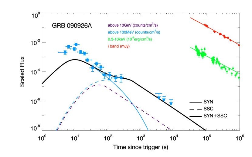
For in the range of , the required density is . Therefore, only when the density is sufficiently high, the SSC emission can explain the 10-100 GeV photons detected during the early afterglow. For GRB 090902B, however, modelling of the broadband (from radio to GeV) afterglows gives a low value for the circumburst density with (Liu & Wang 2011; Barniol Duran & Kumar 2010; Cenko et al. 2011; Lemoine et al. 2013), so the 30 GeV photon detected at 80 s after the trigger can not be interpreted as of SSC origin 222 As discussed in Lemoine et al. (2013), a wind model does not provide as good a match to the data as a constant density medium for this burst, however it leads to a relatively high external wind parameter, for which SSC emission is expected to contribute significantly to the flux at GeV; in this case, it might be possible to accommodate the origin of this highest energy photon with the SSC model.. For GRB 090926A, because there is no radio flux constraint on the parameters, a high density is allowed by the broadband data. We perform a broad-band fitting of GRB 090926A, including one 20 GeV photon at 25 s after the burst, as shown in Fig.3. The SSC component at energies above 100 MeV becomes dominant after 100 s after the trigger. At energies above 10 GeV, the SSC component is dominant and peaks at 30-50 s after the trigger, while the synchrotron flux is negligible. Note that the early-time high-energy emission before s should be attributed to the prompt emission.
GRB130427A shows high-energy photons above 100 MeV up to about one day and high-energy photons above 30 GeV after several thousands seconds after the burst (Zhu et al. 2013). The situation is similar to GRB 940217, in which a 18 GeV photon was detected by Energetic Gamma-Ray Experiment Telescope (EGRET), at about 5000 seconds after the burst (Hurley et al. 1994). This poses severe challenge for the synchrotron afterglow model. As such late times, the SSC mechanism is the likely mechanism for 10 GeV photons, corresponding to the case in Fig.1(a).
4.2 External IC of central X-ray emission
During the early afterglow, X-ray emission from the central source has been usually observed by Swift. During the first hundreds of seconds, steeply decaying X-ray emission from the high-latitude region of the emitting shells are common (Tagliaferri et al. 2005). X-ray flares are also common during the early afterglow, with a fraction of (Nousek et al. 2006; Chincarini et al. 2010). We study whether the external IC of the central X-ray emission can explain the 90 GeV photon seen in e.g. GRB 090902B if the surrounding circumburst density is low. We use X-ray flare emission as an illustration.
Assuming that an X-ray flare occurs at s after the burst with a duration of and the peak of the X-ray flare is , the peak of the observed EIC flux is
| (14) |
So this peak energy can reach up to 100 GeV at s after the trigger for typical parameters of LAT GRBs. The X-ray flare photons cause enhanced cooling of electrons through the IC process. According to Wang et al. (2006), when the X-ray flare flux is larger than a critical flux
| (15) |
we have (for ), and thus all the newly shocked electrons will cool, emitting most of their energy into the IC emission. The peak spectral flux of the EIC emission is
| (16) |
where is the correction factor accounting for the suppression of the IC flux due to the anisotropic scattering effect compared to the isotropic scattering case (Fan & Piran 2006; He et al. 2009). Therefore, the photon flux of the EIC emission at for the fast cooling case (i.e., is ( He et al. 2012)
| (17) |
We find that the photon flux is insensitive to the density of the circumburst medium, in stark contrast to the SSC mechanism. With the LAT effective area of for GeV photons, the number of high-energy photons of detected by LAT during the flare period is estimated to be
| (18) |
Thus, for strong GRBs with , the external IC emission could produce 10-100 GeV photons in the presence of strong central X-ray emission, even the density of the circumburst medium is low. This could explain the 90 GeV (in the local redshift frame) photon detected in GRB 090902B at 80 s after the trigger.
5 Discussions and Conclusions
We have shown that, considering the properties of the microturbulence magnetic field in the relativistic GRB afterglow shocks, the maximum synchrotron photon energy produced by shock-accelerated electrons is a few GeV at hundreds of seconds after the burst and this maximum photon energy decreases quickly with time. Thus, the synchrotron afterglow scenario can only explain the extended high-energy emission below several GeV. The fast decrease of the maximum photon energy could lead to a fast decay of the synchrotron light curves, as seen in some Fermi/LAT GRBs.
High energy photons above 10 GeV, seen in some strong GRBs, should have another origin. Inverse-Compton mechanism is the natural mechanism for such photons. The afterglow SSC mechanism is one possible scenario if the circumburst medium density is sufficiently large (i.e. typically ), which may explain GeV photons in a few cases, such as GRB 090926A and GRB130427A. An alternative mechanism is the external IC of central X-ray emission, such as X-ray flares or prompt high-latitude X-ray emission, since the IC flux from this process is insensitive to the density of the circumburst medium and that central X-ray emission is common during the early afterglows. Interestingly, this scenario has been supported by the simultaneous detections of X-ray flares (by Swift) and GeV emission (by Fermi LAT) in GRB 100728A (Abdo et al. 2011b; He et al. 2012).
High energy photons above 10 GeV have also been detected from GRBs during the prompt phase, such as in GRB080916C and GRB090510. As the high-energy emission lies at the extrapolation of the Band high-energy component, e.g. in GRB080916C (Abbo et al. 2009c), it was suggested that these high energy photons could be produced by synchrotron radiation in the Bohm regime (Wang et al. 2009). Since the internal shock/dissipation mechanism that produces the prompt emission involves mildly relativistic shocks in a possibly magnetized environment, the physics of acceleration is expected to be different, and the Bohm acceleration may be possible for the highest electrons producing the prompt GeV photons.
References
- (1) Abdo, A. A., et al. 2009a, ApJ, 706, L138
- (2) Abdo, A. A., et al. 2009b, Nature, 462, 331
- (3) Abdo, A. A., et al. 2011a, ApJ, 729, 114
- (4) Abdo A., et al. 2011b, ApJ, L27
- (5) Ackermann M., et al. 2013, arXiv:1303.2908
- (6) Barniol Duran, R.; Kumar, P., 2011, MNRAS, 412, 522
- (7) Chang, P., Spitkovsky, A., Arons, J., 2008, ApJ, 674, 378
- (8) Chincarini, G.; Mao, J.; Margutti, R.; et al., 2010, MNRAS, 406, 2113
- (9) Fan, Y., & Piran, T. 2006, MNRAS, 370, L24
- (10) Ghisellini, G., Ghirlanda, G., Nava, L., & Celotti, A. 2010, MNRAS, 403, 926
- (11) Gruzinov, A., Waxman, E., 1999, ApJ, 511, 852
- (12) He, H. N., Wang, X. Y., Yu, Y.W., & Mészáros, P. 2009, ApJ, 706, 1152
- (13) He, H. N., Wu, X. F., Toma, K., Wang, X. Y., & Mészáros, P. 2011, ApJ, 733, 22
- (14) He, H. N., Zhang, B. B., Wang, X. Y. et al. 2012, ApJ, 753, 178
- (15) Hurley, K., et al. 1994, Nature, 372, 652
- (16) Keshet, U., Katz, B., Spitkovsky, A., & Waxman, E., 2009, ApJ, 693, L127
- (17) Kirk, J. G., Reville, B., 2010, ApJ, 710, 16
- (18) Kumar, P., & Barniol Duran, R. 2009, MNRAS, 400, L75
- (19) Kumar, P., & Barniol Duran, R. 2010, MNRAS, 409, 226
- (20) Kumar, P. Hernandez, R. A.; Bosnjak, Z.; Duran, R. Barniol, 2012, MNRAS, 427, L40
- (21) Lemoine, M. 2013, MNRAS, 428, 845
- (22) Lemoine, M., Li, Z., Wang, X. Y., 2013, arXiv:1305.3689
- (23) Liu, R. Y., & Wang, X. Y., 2011, ApJ, 730, 1
- (24) Medvedev, M. V. & Loeb, A., 1999, ApJ, 526, 697
- (25) Nousek, J., et al. 2006, ApJ, 642, 389
- (26) Piran, T., & Nakar, E. 2010, ApJ, 718, L63
- (27) Plotnikov, I., Pelletier, G., Lemoine, M., 2013, MNRAS, 430, 1208
- (28) Sagi, E., Nakar, E., 2012, ApJ, 749, 80
- (29) Tagliaferri, G., et al. 2005, Nature, 436, 985
- (30) Wang, X. Y., Li, Z., & Mészáros, P. 2006, ApJ, 641, L89
- (31) Wang, X. Y., Li, Z., Dai, Z. G., & Mészáros, P. 2009, ApJ, 698, L98
- (32) Wang, X. Y., He, H. N., Li, Z., Wu, X. F., & Dai, Z. G. 2010, ApJ, 712, 1232
- (33) Zhang, B., & Mészáros, P., 2001, ApJ, 559, 110
- (34) Zhu, S. et al., 2013, GCN Circular number 14471