Dynamics and emission of wind-powered afterglows of gamma-ray bursts: flares, plateaus and steep decays

Abstract

We develop a model of early X-ray afterglows of gamma-ray bursts originating from the reverse shock (RS) propagating through ultra-relativistic, highly magnetized pulsar-like winds produced by long-lasting central engines. We first perform fluid and MHD numerical simulations of relativistic double explosions. We demonstrate that even for constant properties of the wind a variety of temporal behaviors can be produced, depending on the energy of the initial explosion and the wind power, the delay time for the switch-on of the wind, and magnetization of the wind. X-ray emission of the highly magnetized RS occurs in the fast cooling regime - this ensures high radiative efficiency and allows fast intensity variations. We demonstrate that: (i) RS emission naturally produces light curves showing power-law temporal evolution with various temporal indices; (ii) mild wind power, of the order of $\sim 10^{46}$ erg s^-1 (equivalent isotropic), can reproduce the afterglows’ plateau phase; (iii) termination of the wind can produce sudden steep decays; (iv) short-duration afterglow flares are due to mild variations in the wind luminosity, with small total injected energy.

1. Introduction

Gamma-ray bursts (GRBs) are produced in relativistic explosions (Paczynski, 1986; Piran, 2004) that generate two shocks: forward shock and reversed shock. The standard fireball model (Rees & Meszaros, 1992; Sari & Piran, 1995; Piran, 1999; Mészáros, 2006) postulates that the prompt emission is produced by internal dissipative processes within the flow: collisions of matter-dominated shells, Piran (1999), or reconnection events (Lyutikov, 2006b)). The afterglows, according to the fireball model, are generated in the external relativistic blast wave.

Since emission from the forward shock depends on “integrated properties” (total injected energy and total swept-up mass), the corresponding light curves were expected to be fairly smooth. In contrast, observations show the presence of unexpected features like flares and light curves plateaus (Nousek et al., 2006; O’Brien et al., 2006; Gehrels & Razzaque, 2013; Lien et al., 2016; de Pasquale et al., 2007; Chincarini et al., 2010; Mazaeva et al., 2018), abrupt endings of the plateau phases (Troja et al., 2007), fast optical variability (e.g. GRB021004 and most notoriously GRB080916C), missing (De Pasquale et al., 2016) and chromatic (Panaitescu, 2007; Racusin et al., 2009) jet breaks, missing reverse shocks (Gomboc et al., 2009)). These phenomena are hard to explain within the standard fireball model that postulates that the early $X$-ray are produced in the forward shock, as argued by (Lyutikov, 2009; Kann et al., 2010; Lyutikov & Camilo Jaramillo, 2017).

The origin of sudden drops in afterglow light curves is especially mysterious. As an example, GRB 070110 starts with a normal prompt emission, followed by an early decay phase until approximately 100 seconds, and a plateau until $\sim 10^{4}$ s. At about $2\times 10^{4}$ seconds, the light curve of the afterglow of GRB 070110 drops suddenly with a temporal slope $>7$ (Sbarufatti et al., 2007; Krimm et al., 2007a, b; Troja et al., 2007).

Observations of early afterglows in long Gamma Ray Bursts (GRBs), at times $\leq$ 1 day, require a presence of long-lasting active central engine. Previously, some of the related phenomenology was attributed to long lasting central engine (see §2 for a more detailed discussion of various models of long-lasting central engine). A number of authors discussed long-lasting engine that produces colliding shells, in analogy with the fireball model for the prompt emission (Rees & Meszaros, 1994; Panaitescu et al., 2006; Uhm & Beloborodov, 2007; Barkov & Komissarov, 2010; Barkov & Pozanenko, 2011). The problem with this explanation is that energizing the forward shock requires a lot of energy: the total energy in the blast needs to increase linearly with time, hence putting exceptional demands on the efficiency of prompt emission (Panaitescu et al., 2006; Oates et al., 2007; de Pasquale et al., 2009). In addition, to produce afterglow flares in the forward shock the total energy in the explosion needs to roughly double each time: hence the total energy grows exponentially for bursts with multiple flares.

As an alternative, Lyutikov & Camilo Jaramillo (2017) developed a model of early GRB afterglows with dominant $X$-ray contribution from the reverse shock (RS) propagating in highly relativistic (Lorentz factor $\gamma_{w}\sim 10^{4}-10^{6}$) magnetized wind of a long-lasting central engine; we will refer to this types of model as ”a pulsar paradigm”, stressing similarities to physics of pulsar winds.

Pulsar wind Nebulae (PWNe) are efficient in converting spindown energy of the central objets, coming out in a form of the wind, into high energy radiation, reaching efficiencies of tens of percent (e.g. Kennel & Coroniti, 1984b; Kargaltsev & Pavlov, 2008). This efficiency is much higher that what would have been expected from simple sigma-scaling of dissipation at relativistic shocks (Kennel & Coroniti, 1984a). Effects of magnetic dissipation contribute to higher efficiency (Sironi & Spitkovsky, 2011; Porth et al., 2014).

Lyutikov & Camilo Jaramillo (2017) adopted the pulsar wind model to the case of preceding expanding GRB shock. The model reproduces, in a fairly natural way, the overall trends and yet allows for variations in the temporal and spectral evolution of early optical and $X$-ray afterglows. The high energy and the optical synchrotron emission from the RS particles occurs in the fast cooling regime; the resulting synchrotron power $L_{s}$ is a large fraction of the wind luminosity (high-sigma termination shocks propagate faster through the wind, boosting the efficiency.)

Thus, plateaus - parts of afterglow light curves that show slowly decreasing spectral power - are a natural consequence of the RS emission. Contribution from the forward shock (FS) is negligible in the $X$-rays, but in the optical both FS and RS contribute similarly (but see, e.g., Warren et al., 2017, 2018; Ito et al., 2019): the FS optical emission is in the slow cooling regime, producing smooth components, while the RS optical emission is in the fast cooling regime, and thus can both produce optical plateaus and account for fast optical variability correlated with the $X$-rays, e.g., due to changes in the wind properties. The later phases of pulsar wind interaction with super nova remnant discussed by Khangulyan et al. (2018).

The goal of the present work is two-fold. First, we perform a number of numerical simulations for the propagation of a highly relativistic magnetized wind that follows a relativistic shock wave. Previously, this problem was considered analytically by Lyutikov (2017). Second, we perform radiative calculations of the early X-ray afterglow emission coming from the ultra-relativistic RS of a long-living central engine. We demonstrate that this paradigm allows us to resolve the problems of plateaus, sudden intensity drops, and flares. Qualitatively, at early times, a large fraction of the wind power is radiated: this explains the plateaus. If the wind terminates, so that the emission from RS ceases instantaneously, this will lead to a sharp decrease in observed flux (since particles are cooling fast). Finally, variations of the wind intensity can produce flares that bear resemblance to the ones observed in GRBs.

We argue in this paper that abrupt declines in afterglow curves can be explained if emission originates in the ultra-relativistic and highly magnetized reverse shock of a long-lasting engine. Lyutikov & Camilo Jaramillo (2017) (see also Lyutikov, 2017) developed a model of early GRB afterglows with dominant X-ray contribution from the highly magnetized ultra-relativistic reverse shock (RS), an analog of the pulsar wind termination shock. The critical point is that emission from the RS in highly magnetized pulsar-like wind occurs in the fast cooling regime. Thus it reflects instantaneous wind power, not accumulated mass/energy, as in the case of the forward shock. Thus, it is more natural to produce fast variation in the highly magnetized RS.

2. Models of long-lasting winds in GRBs

The model of Lyutikov & Camilo Jaramillo (2017), explored in more details here, differs qualitatively from a number of previous works that advocated a long lasting central engine in GRBs. Previous works can be divided into two categories. First type of models involves modifying the properties of the forward shock (FS) (e.g. re-energizing of the FS by the long-lasting wind in an attempt to produce flares Rees & Mészáros, 1998; Dai & Lu, 1998; Panaitescu et al., 1998; Dai, 2004). The second type of models assume a long lasting central engine that produces mildly relativistic matter-dominated winds (Sari & Piran, 1999; Genet et al., 2007; Uhm & Beloborodov, 2007; Komissarov & Barkov, 2009; Uhm et al., 2012; Hascoët et al., 2017). In these types of mode the emission is produced in a way similar to the internal shock model for the prompt emission (that is, collision of baryon-dominated shells, amplification of magnetic field and particle acceleration).

The FS-based models encounter a number of fundamental problems (Lyutikov, 2009; Uhm & Beloborodov, 2007) (Though see Lyons et al., 2010; Rowlinson et al., 2010; Resmi & Zhang, 2016; Beniamini & Mochkovitch, 2017; Rowlinson et al., 2013; van Eerten, 2014; Khangulyan et al., 2020; Warren et al., 2020). The key problem is that the properties of the forward shock are “cumulative”, in a sense that its dynamics depend on the total swept-up mass and injected energy, which is impossible to change on a short time scale. For example, to produce a flare within the FS model, the total energy of the shock should increase substantially (e.g., by a factor of two). To produce another flare, even more energy need to be injected, leading to the exponentially increasing total energy with each flare.

Most importantly, the FS-based models cannot produce abrupt steep decays. Such sharp drops require (at the least) that the emission from the forward shock (FS) switches off instantaneously. This is impossible. First, the microphysics of shock acceleration is not expected to change rapidly (at least we have no arguments why it should).

Second, the variations of hydrodynamic properties of the FS, as they translate to radiation, are also expected to produce smooth variations (Gat et al., 2013). As an example, consider a relativistic shock that breaks out from a denser medium (density $n_{1}$) into the less dense one (density $n_{2}\ll n_{1}$). In the standard fireball model total synchrotron power $P_{s}$ per unit area of the shock scale as (Piran, 2004)

$$P_{s}\propto n\Gamma^{2}\gamma^{\prime 2}B^{\prime 2}\propto n^{2}\Gamma^{6}\mbox{}$$

$$\gamma^{\prime}\propto\Gamma\mbox{}$$

$$B^{\prime}\propto\Gamma\sqrt{n}$$ (1)

where $\Gamma$ is the Lorentz factor of the shock, $\gamma^{\prime}$ is the Lorentz factor of accelerated particles.

Importantly, if a shock breaks out from a dense medium into the rarefied one, with $n_{2}\ll n_{1}$, it accelerates to approximately $\Gamma_{2}\approx\Gamma_{1}^{2}$, as the post-shock internal energy in the first medium is converted into bulk motion (Johnson & McKee, 1971; Lyutikov, 2010). Thus a change in power and peak frequency scale as

$$\frac{P_{s,2}}{P_{s,1}}={\Gamma_{1}^{6}}\left(\frac{n_{2}}{n_{1}}\right)^{2}$$ (2)

Thus, even though we assumed $n_{2}\ll n_{1}$, the synchrotron emissivity in the less dense medium is largely compensated by the increase of the Lorentz factor. Since the expected Lorentz factor at the time of sharp drops is $\Gamma_{1}\sim$ few tens, suppression of emission from the forward shock requires the unrealistically large decrease of density.

Oganesyan et al. (2020) discussed appearance of plateaus from an off-axis jet (so that a more energetic part of the FS becomes visible and effectively boosts the observed flux. We expect though that at observer times of few$\times 10^{4}$ seconds the X-ray emitting particles in the FS are in the slow cooling regime, liming how short time scales in the observed emission light curves can be produced.

The model of Lyutikov & Camilo Jaramillo (2017), and the present investigation, is more aligned with the previously discussed emission from the RS (Sari & Piran, 1999; Genet et al., 2007; Uhm & Beloborodov, 2007; Uhm et al., 2012; Hascoët et al., 2017). But the present model is qualitatively different: emission properties here are parametrized within the pulsar wind paradigm of Kennel & Coroniti (1984b), not the fireball model (e.g. Piran, 2004). Qualitatively, the advantage of the present model of the highly magnetized/highly relativistic RS emission over the fireball adaptation to the RS case are similar to the prompt emission: high magnetized relativistic flows can be more efficient in converting the energy of the explosion to radiation, as they do not “lose” energy on the bulk motion of non-emitting ions (Lyutikov & Blandford, 2003; Lyutikov, 2006b).

The pulsar wind paradigm of Kennel & Coroniti (1984b) also has a very different prescription for particle acceleration and emission: it relates the typical (minimum) Lorentz factor of the accelerated particles to the Lorentz factor of the pre-shock wind $\gamma_{min}\sim\gamma_{w}$ with $\gamma_{w}\sim 10^{4}-10^{6}$), while the magnetic field in the emission region follows the shock compression relations. In contrast, the fireball model parametrizes both the Lorentz factor of the accelerated particles and the (shock-amplified) magnetic field to the upstream properties of the baryon-dominated energy flow (e.g., $\gamma_{min}\sim\epsilon_{e}(m_{p}/m_{e})\gamma_{w}$ with $\gamma_{w}\sim 10^{2}$). The resulting emission properties are qualitatively different.

3. Relativistic double explosion

3.1. Triple shock structure

Consider relativistic point explosion of energy $E_{1}$ in a medium with constant density $\rho_{ex}=m_{p}n_{ex}$, followed by a wind with constant luminosity $L_{w}$ (Lyutikov, 2017, both $E_{1}$ and $L_{w}$ are isotropic equivalent values). The initial explosion generates a Blandford-McKee forward shock wave (BMFS) Blandford & McKee (1976)

$$\Gamma_{1}=\sqrt{\frac{17}{8\pi}}\sqrt{\frac{E_{1}}{\rho_{ex}c^{5}}}t^{-3/2}\mbox{}$$

$$p_{1}=\frac{2}{3}\rho_{ex}c^{2}\Gamma_{1}^{2}f_{1}(\chi)\mbox{}$$

$$\gamma^{2}_{1}=\frac{1}{2}\Gamma_{1}^{2}g_{1}(\chi)\mbox{}$$

$$n_{1}=2n_{ex}\Gamma_{1}n_{1}(\chi)\mbox{}$$

$$f_{1}(\chi)=\chi^{-17/12}\mbox{}$$

$$g_{1}(\chi)=1/\chi\mbox{}$$

$$n_{1}(\chi)=\chi^{-5/4}\ \mbox{}$$

$$\chi=\left[1+2(m+1)\Gamma^{2}\right]\left(1-r/t\right)$$ (3)

Subscript $ex$ indicates the properties in the surrounding medium; subscript $1$ indicates that quantities are measured behind the leading BMFS, hence between the two forward shocks; The Lorentz factor $\Gamma$ depends on time as $\Gamma^{2}\propto t^{-m}$, $m=3$.

We assume that the initial GRB explosion leaves behind an active remnant - a black hole or (fast rotating) neutron star. The remnant produces a long-lasting pulsar-like wind, either using the rotational energy of the newly born neutron star (Usov, 1992; Komissarov & Barkov, 2007), accretion of the pre-explosion envelope onto the BH (Cannizzo & Gehrels, 2009), or if the black hole can keep its magnetic flux for sufficiently long time (Komissarov & Barkov, 2009; Barkov & Komissarov, 2010; Lyutikov, 2011; Lyutikov & McKinney, 2011).

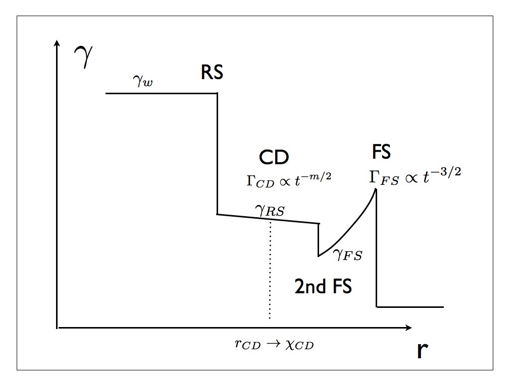
One expects that the central engine produces very fast and light wind that will start interacting with the slower, but still relativistically expanding, ejecta. As the highly relativistic wind from the long-lasting engine interacts with the initial explosion, it launches a second forward shock in the medium already shocked by the primary blast wave. At the same time the reverse shock forms in the wind; the two shocks are separated by the contact discontinuity (CD), Figure 1.

Figure 1.— Velocity structure of the triple-shock configuration. Leading is the FS that generates a self-similar post-shock velocity and pressure profiles. A fast wind with Lorentz factor $\gamma_{w}$ is terminated at the reverse shock (RS); the post-RS flow connects through the contact discontinuity (CD, dotted line) to the second shock driven in the already shock media. The CD is located at $r_{\rm CD}$, corresponding to $\chi_{\rm CD}$. The RS and the second forward shock (2nd FS) are located close to $\chi_{\rm CD}$ (Lyutikov & Camilo Jaramillo, 2017).

First, we assume that external density is constant, while the wind is magnetized with constant luminosity (variations in wind luminosity are explored in §5)

$$L_{w}=4\pi\gamma_{w}^{2}\left(\rho_{w}c^{2}+\frac{B_{w}^{2}}{4\pi}\right)r^{2}c$$ (4)

where $\rho_{w}$ and $B_{w}$ are density and magnetic field measured in the wind rest frame. Thus

$$B_{w}=\sqrt[]{\frac{\sigma_{w}}{1+\sigma_{w}}}\ \sqrt[]{\frac{L_{w}}{c}}\frac{1}{r\gamma_{w}}$$ (5)

where

$$\sigma_{w}=\frac{B^{2}_{w}}{4\pi\rho_{w}c^{2}}.$$ (6)

is the wind magnetization parameter (Kennel & Coroniti, 1984a). In our “pulsar wind” paradigm, we assume that the mass loading of the wind is very small, while the the wind is assumed to be very fast, with $\gamma_{w}\gg\Gamma_{FS},\,\Gamma_{\rm CD}$.

3.2. Analytical expectations: self-similar stages

Generally, the structure of the flows in double explosions is non-self-similar (Lyutikov, 2017). First, with time the second forward shock approaches the initial forward shock (FS); for sufficiently powerful winds the second FS may catch up with the primary FS. The presence of this special time violates the assumption of self-similarity. We can estimate the catch-up time by noticing that the power deposited by the wind in the shocked medium scales as $L_{w}/\Gamma_{\rm CD}^{2}$. Thus, in coordinate time the wind deposits energy similar to the initial explosion at time when $\Gamma_{\rm CD}\sim\Gamma_{FS}$,

$$t_{eq}=\Gamma_{FS}^{2}\frac{E_{1}}{L_{w}}\propto\left(\frac{E_{1}^{2}}{c^{5}\rho L_{w}}\right)^{1/4}=2\times 10^{7}\;E_{1,52}^{1/2},L_{w,46}^{-1/4}n^{-1/4}\mbox{ sec},$$ (7)

almost a year in coordinate time. At times $t\leq t_{eq}$ the second shock is approximately self-similar, the CD is located far downstream of the first shock; and is moving with time in the self-similar coordinate $\chi$, associated with the primary shock, towards the first shock. The motion of the first shock is unaffected by the wind at this stage. At times $t\geq t_{eq}$ the two shocks merge - the system then relaxes to a Blandford-McKee self-similar solution with energy supply.

In the numerical estimate in (7) we used the wind power $L_{w}\sim 10^{46}$ erg s^-1 which at first glance may look too high. Indeed, the total energy budget for isotropic wind is then $E_{w}\sim L_{w}t_{eq}\sim 10^{53}$ ergs, this value is much larger rotating energy of fast spinning NS $\sim 10^{52}$ erg. But recall that this is an isotropic equivalent power. In the case of long GRBs, both the initial explosion and the power of the long-lived central engine are collimated into small angle $\theta\sim 0.1$ rad (e.g. Komissarov & Barkov, 2007). After jet-break out the opening angle remains nearly constant. Thus, the true wind power can be estimated as $L_{w,true}\approx\theta^{2}L_{w}/2\sim 10^{44}$ erg/s and $E_{w}\sim 10^{51}$ ergs, which is an allowed energy budget of fast spinning NS.

Secondly, the self-similarity may be violated at early times if there is an effective delay time $t_{d}$ between the initial explosion and the start of the second wind. (This issues is also important in our implementation scheme, §4 - since we start simulation with energy injection at some finite distance from the primary shock this is equivalent to some effective time delay for the wind turn-on.)

Suppose that the secondary wind turns on at time $t_{d}$ after the initial one and the second shock/CD is moving with the Lorentz factor

$$\Gamma_{\rm CD}^{2}\propto(t-t_{d})^{-m}$$ (8)

Then, the location of the second shock at time $t$ is

$$R_{\rm CD}=(t-t_{d})\left(1-\frac{1}{2\Gamma_{\rm CD}^{2}(m+1)}\right)$$ (9)

The corresponding self-similar coordinate of the second shock in terms of the primary shock self-similar parameter $\chi$ is

$$\chi_{\rm CD}=\left(1+8\Gamma_{1}^{2}\right)\left(1-\frac{R}{t}\right)\approx\left(\frac{8t_{d}}{t}+\frac{4}{(m+1)\Gamma_{\rm CD}^{2}}\right)\Gamma_{1}^{2}$$ (10)

The effective time delay $t_{d}$ introduces additional (beside the catch-up time (7)) time scales in the problem. Thus, even within the limits of expected self-similar motion, $t\ll t_{eq}$ the effective delay time $t_{d}$ violates the self-similarity assumption. Still, depending on whether the ratio $t_{d}/(t\Gamma_{\rm CD}^{2})$ is much larger or smaller than unity, we expect approximately self-similar behavior (Lyutikov, 2017; Lyutikov & Camilo Jaramillo, 2017)

For $t_{d}\geq t/(2(m+1)\Gamma_{\rm CD}^{2})$, the location of the CD in the self-similar coordinate associated with the first shock is

$$\chi_{\rm CD}\approx\frac{8\gamma_{1}^{2}{t_{d}}}{t}\propto t^{-4}$$ (11)

$$\Gamma_{\rm CD}=0.52\frac{E_{1}^{5/48}{t_{d}}^{5/48}{L_{w}}^{1/4}}{c^{85/48}\rho^{17/48}t^{11/12}}$$ (12)

Alternatively, for $t_{d}\leq t/(2(m+1)\Gamma_{\rm CD}^{2})$,

$$\chi_{\rm CD}=2.68\left(\frac{E_{1}}{c^{5/2}\sqrt{\rho}t^{2}\sqrt{L_{w}}}\right){}^{24/29}$$ (13)

$$\Gamma_{\rm CD}=0.50\frac{E_{1}^{5/58}L_{w}^{6/29}}{c^{85/58}\rho^{17/58}t^{39/58}}$$ (14)

Finally, if the second explosion is point-like with energy $E_{2}$, the Lorentz factor of the second shock evolves according to (Lyutikov, 2017)

$$\gamma_{2}=\sqrt{\frac{71}{2}}\left(\frac{17}{\pi}\right)^{5/24}\left(\frac{{E_{1}}^{5}{t_{d}}^{5}}{c^{85}(m_{p}n_{ex})^{17}}\right)^{1/24}\sqrt{E_{2}}t^{-7/3}$$ (15)

(this expression is applicable for $t\leq\Gamma_{1}^{2}t_{d}$, the time when the second shock catches with the primary shock.

Relation (12-15) indicate that depending on the particularities of the set-up, we expect somewhat different scalings for the propagation of the second shock (we are also often limited in integration time to see a switch between different self-similar regimes).

The point of the previous discussion is that mild variations between the properties of double explosions (delay times, luminosity of the long lasting engine) are expected to produce a broad variety of behaviors, like various power-law indices and temporarily changing overall behavior. This ability of the model to accommodate a fairly wide range of behaviors with minimal numbers of parameters is important in explaining highly temporally variable early afterglows, as we further explore in this paper.

4. Numerical simulations of relativistic double explosions

4.1. Simulations’ setup

Figure 2.— Hydrodynamic simulations of the double explosion. Potted are Lorentz factor and tracer distribution as a function of radius at the moment $t=1.9\;[r_{s}/c]$. The tracer distinguishes the wind from the shocked external medium. The parameters for each panel are encoded in the titles, Table 1.

Figure 3.— Self-similar coordinate of the second shock $\chi$, eq (10), as function of time for different models. Plotted are values of $8t_{\rm d}/t$ from simulation (triangles), analytical curve (crosses) Lyutikov (2017). Also plotted square of inverse Lorentz factor (diamonds). Models with high wind power $pm0$ and $pp2$ closely follow the theoretical curve.

Figure 4.— Lorentz factor of the CD as function on time – triangles and analytical expectations Lyutikov (2017). The jumps in the Lorentz factor at later times occurs when the wind driven FS catches with the leading BMFS.

Figure 5.— Lorentz factor of contact discontinuity as functions of time . The analytical estimations (see Eq.12) $\Gamma_{\rm CD}\propto t^{-0.92}$ and for wind driven shock $\Gamma_{\rm CD}\propto t^{-0.5}$ (see thin lines with crosses, stars abd circles). We calculate the power indexes on stright parts of the curves, $\log_{10}t>0.3$.

Figure 6.— Dependence of the Lorentz factor of the contact discontinuity at $t=2[R_{\rm s}/c]$. In the high wind power regime the scaling is close to the expected $\Gamma_{\rm CD}\propto L_{w}^{1/4}$, Eq. (12).

Figure 7.— Time dependence of $\chi_{\rm CD}$ of contact discontinuity. We calculate the power indexes on stright parts of the curves, $\log_{10}t>0.2$.

Figure 8.— Dependence of the power slop $\alpha_{\chi}$ at $t=2[R_{\rm s}/c]$.

The simulations were performed using a one dimensional (1D) geometry in spherical coordinates using the PLUTO code (Mignone et al., 2007). Spatial parabolic interpolation, a 3rd order Runge-Kutta approximation in time, and an HLLD Riemann solver were used (Mignone et al., 2009). PLUTO is a modular Godunov-type code entirely written in C and intended mainly for astrophysical applications and high Mach number flows in multiple spatial dimensions. The simulations were run through the MPI library in the DESY (Germany) cluster. The flow has been approximated as an ideal, relativistic adiabatic gas with and without the toroidal magnetic field, one particle species, and polytropic index of 4/3. The adopted resolution is $192000$ cells. The size of the domain is $r\in[0.95,4]R_{\rm s}$ or $r\in[0.98,4]R_{\rm s}$, here $R_{\rm s}$ is initial position of shock wave front.

As initial condition we set solution of B&Mc with shock radius 1, Eq (3), the Lorentz factor of the shock was 15. The external matter was assumed uniform with density $\rho=1$ and pressure $p=10^{-4}$ (in units $c=1$). The pressure and density just after shock was determined by B&Mc solution ($\rho_{\rm BM}=42.43$ and $p_{\rm BM}=150$) with total energy $E_{\rm BM}=2.13\times 10^{5}$. From the left boundary (from a center) at radius $r_{\rm w}=0.95$ or $r_{\rm w}=0.98$ (models marked by letter ’s’ at the end of its name) was injected wind with initial Lorentz factor $\gamma_{\rm w}=50$, the pressure of the wind was fixed $p_{w}=10^{-3}\rho_{w}c^{2}$. The parameters of the models are listed in Table 1.

The chosen setup corresponds to the following physical parameters: the density unit $n_{ISM}=1/{\rm cm}^{3}$, total isotropic explosion energy $E_{ISO}=1.5\times 10^{52}$ ergs, laboratory time $t_{lab}=R_{s}/c=10^{7}$ s, the initial radius of the shock $R_{s}=3\times 10^{17}$ cm and observer time $t_{obs}=4.4\times 10^{3}$ s. The isotropic wind power unit is $L_{w,0}=1.2\times 10^{47}$ erg/s.

We performed nine runs without magnetic field and eight runs with different magnetizations. Our numerical model for the primary shock is consistent with analytical solution of BM with an accuracy $\sim 10$% (pressure, density and maximal Lorentz factor). On the top of each panel of Figures (2)–(10) we indicate name of the model with parameters presented in the Table 1.

4.2. Results: long-term dynamics of double explosions

4.2.1 Unmagnetized secondary wind

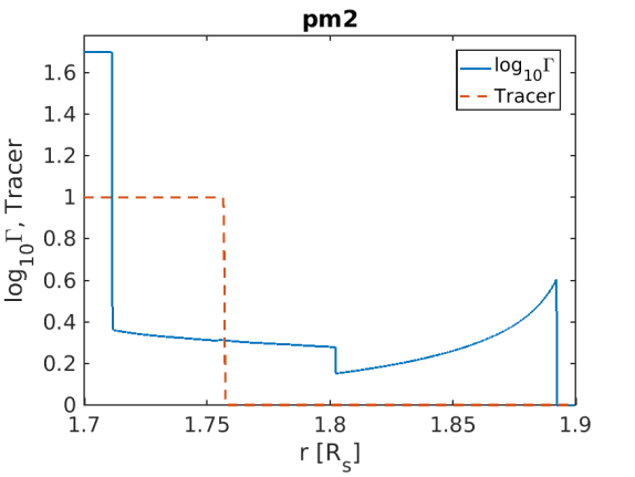
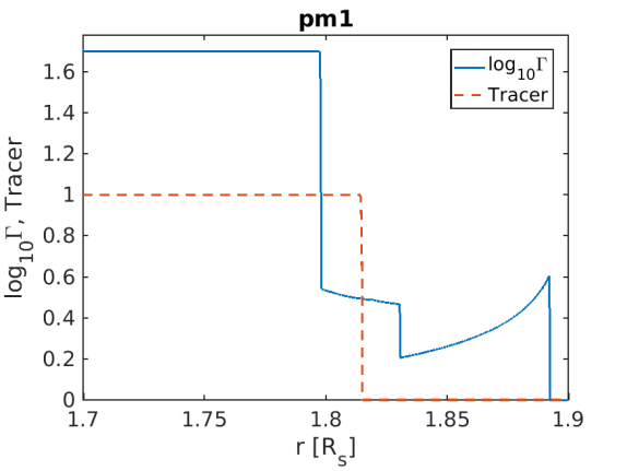
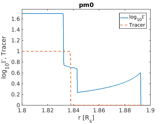
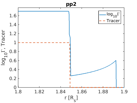
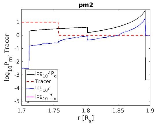
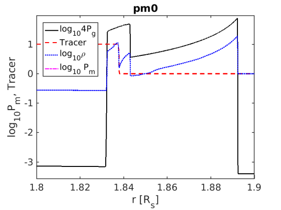
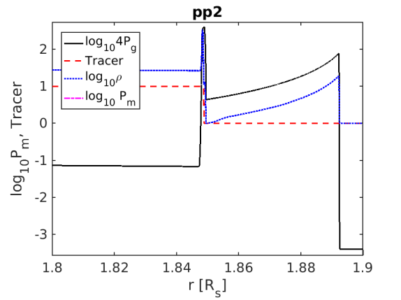
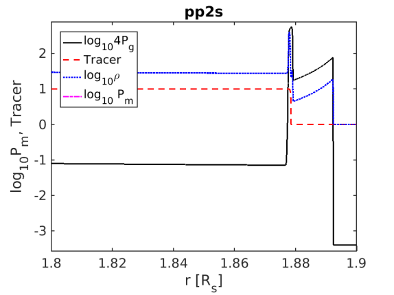
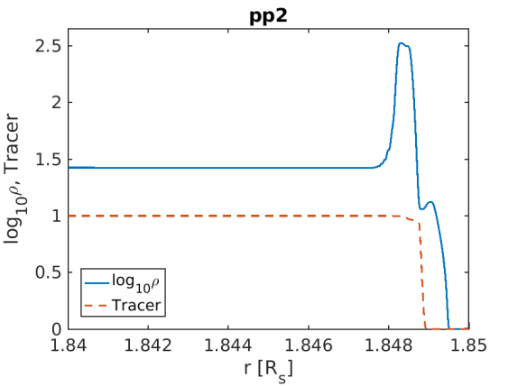
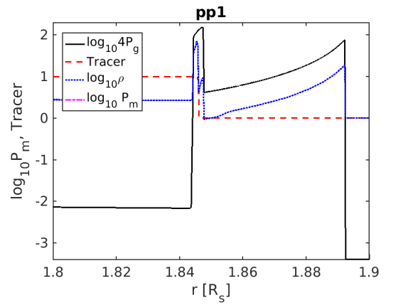
In the unmagnetized models labeled pXX, we vary wind density. The wind density vary from $10^{-4}$ for pm4 model to $10^{2}$ for pp2. In Figure (2) we plot the results of pXX models there we vary power of hydrodynamical wind. At small radius one can clearly identify the location of the reverse shock (RS), where the Lorentz factor suddenly drops. At larger radius the contact discontinuity (CD) is identified by the the position of the tracer drop. Further out is the secondary forward shock, and the initial BM shock. More curves can be seen in the Appendix A.1.

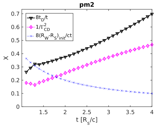
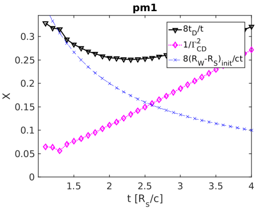
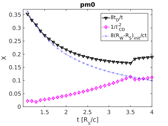
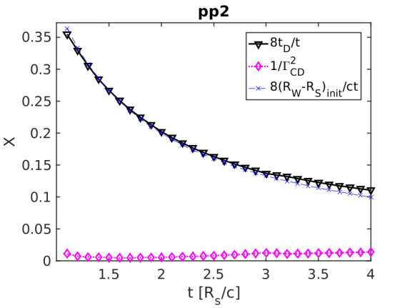
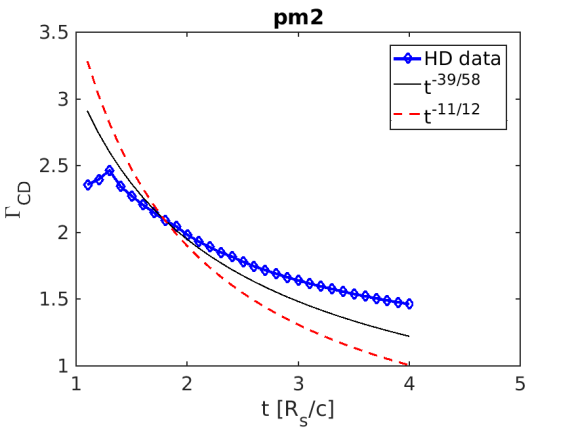
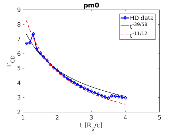
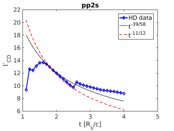
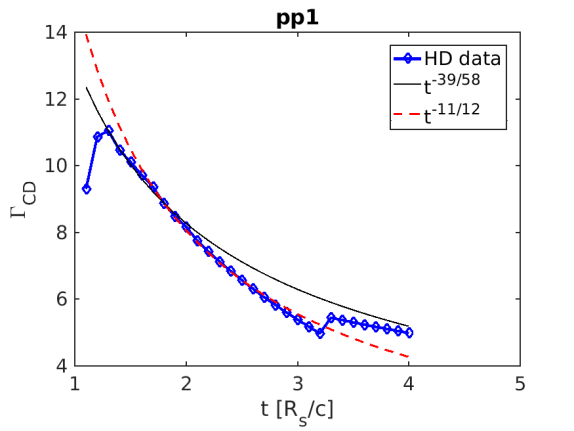
In Figure 3 three curves are shown for pXX models: (i) theoretical curve based on the expectation from the initial conditions $t_{\rm d}=(r_{\rm s}-r_{\rm w})/c$; (ii) Inverse square of Lorentz factor; (iii) actual time of delay calculated from position of CD and its Lorentz factor using eq (10). As we can see in the models $pm0$, $pp1$ and $pp2$ (power of the wind comparable to initial explosion) theoretical and actual curves are close. More powerful wind ($L_{\rm w}r_{\rm s}/c\geq 0.1E_{\rm BM}$) can push CD much faster that allows to satisfy conditions (8). Large value of $\Gamma_{\rm CD}$ also relax applicability condition of (12). So similar picture we can see on Figure 4, here models $pp2,pp1$ and $pm0$ follow theoretically predicted time dependence (see eq (12)) $\Gamma_{\rm CD}\propto t^{-11/12}$. Deviations from theoretical curves on Figures (3) and (4) at the late time are due to the fact that the wind-triggered FS reach the radius of BMFS, affecting the motion of the initial shock: in this case transition to wind-driven BM solution occurs. The Lorentz factor is fitted by power law $\Gamma_{\rm CD}\propto t^{-0.45}$.

Table 1Parameters of the models

Model	$\rho_{\rm w}$	$r_{\rm w}$	$\sigma_{\rm w}$	$L_{\rm w}$ [$L_{w,0}$]
$pm4$	$10^{-4}$	0.95	0	$10^{-4}$
$pm3$	$10^{-3}$	0.95	0	$10^{-3}$
$pm2$	$10^{-2}$	0.95	0	$10^{-2}$
$pm2s$	$10^{-2}$	0.98	0	$10^{-2}$
$pm1$	$10^{-1}$	0.95	0	$10^{-1}$
$pm0$	1	0.95	0	$1$
$pp1$	$10^{1}$	0.95	0	$10^{1}$
$pp2$	$10^{2}$	0.95	0	$10^{2}$
$pp2s$	$10^{2}$	0.98	0	$10^{2}$
$mm1p1$	$10^{1}$	0.95	0.1	$11$
$m0p1$	$10^{1}$	0.95	1.0	$20$
$m05p1$	$10^{1}$	0.95	3.0	$40$
$m1p1$	$10^{1}$	0.95	10	$110$
$mm1ep1$	$9.09$	0.95	0.1	$10^{1}$
$m0ep1$	$5.00$	0.95	1.0	$10^{1}$
$m05ep1$	$2.50$	0.95	3.0	$10^{1}$
$m1ep1$	$0.91$	0.95	10	$10^{1}$

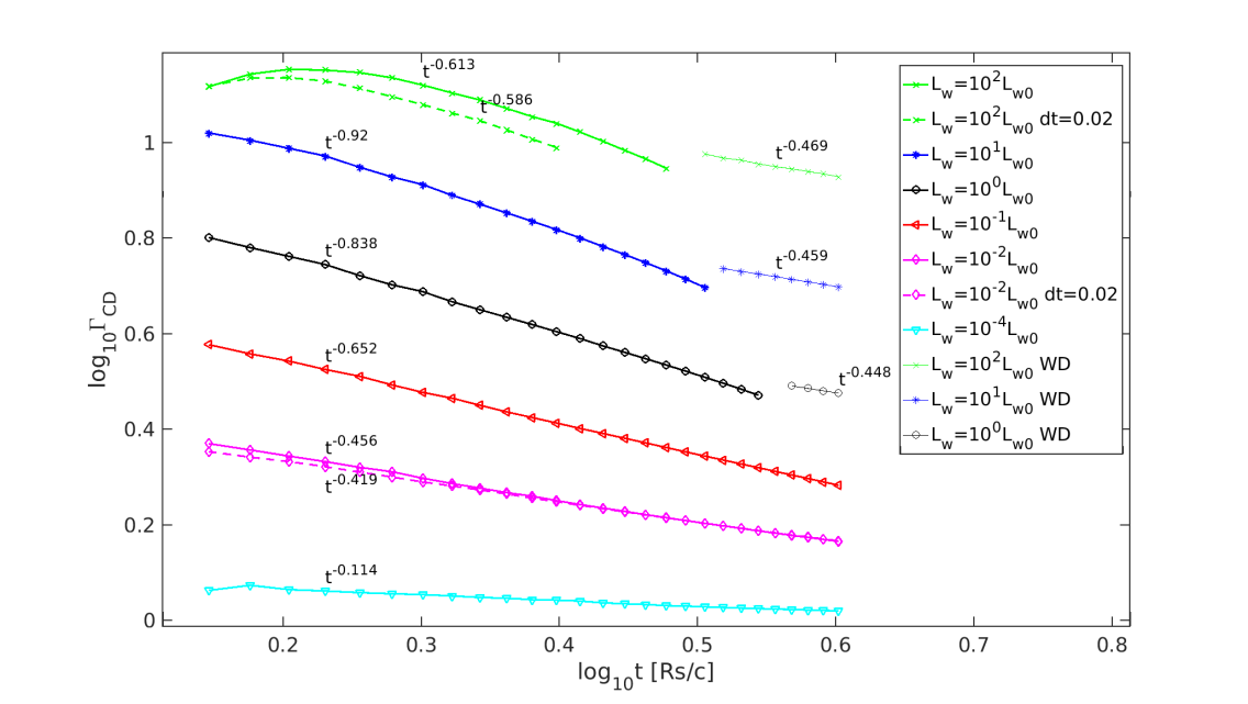
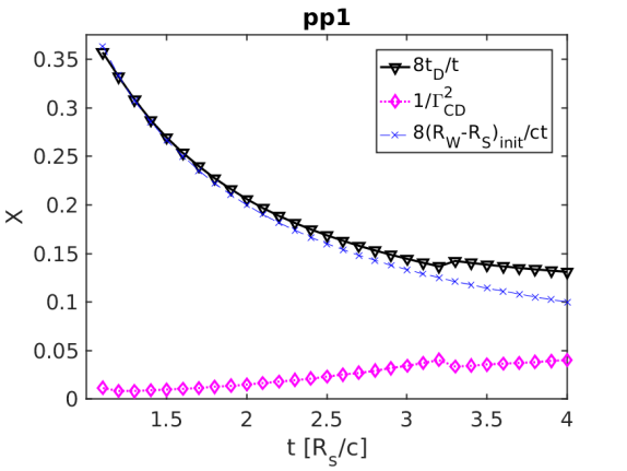
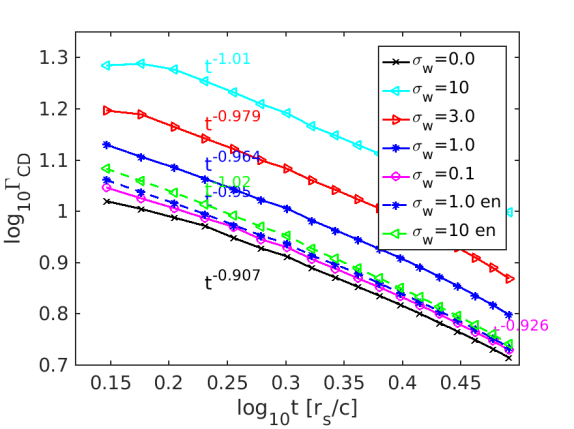
Figure 5 shows time dependence of Lorentz factor at CD and its $\chi_{\rm CD}$. For high relative wind power the slope of Lorentz factor coincide with theoretical one. Moreover, dependence of the theoretical Lorentz factor on wind power (see eq (12)) $\Gamma_{\rm CD}\propto L_{\rm w}^{0.25}$ and simulated one (Figure 6) $\Gamma_{\rm CD}\propto L_{\rm w}^{0.18}$) are in a good agreement.

Time behavior of theoretically predicted $\chi_{\rm CD}$ ($\chi_{\rm CD}\propto t^{\alpha_{\chi}}$, $\alpha_{\chi}=-4$) is in a good agreement with models with high relative wind power, see Figures (7) and (8) which shows tendency of power slop to $\alpha_{\chi}={-3.8}$ at large wind powers. After the moment than wind driven FS reaches BMFS, the slope is changed and tends to $\alpha_{\chi}={-2.7}$.

The deviation from theoretically predicted slop $\Gamma_{\rm CD}\propto t^{-0.92}$ take place when wind power is low. The low power wind forms sub-relativistic shock, which pushes sub-relativistic CD. Since the analytic theory is applicable in ultra relativistic regime, this explains deviations of numerical results from theory for $\Gamma_{CD}<3$. The same effect works for dependence of $\chi_{\rm CD}$ on time. Sub-relativistic motion of CD can have only small values of $\alpha_{\chi}\sim-2$, and powerful winds in relativistic regime shows good agreement with theoretical predictions.

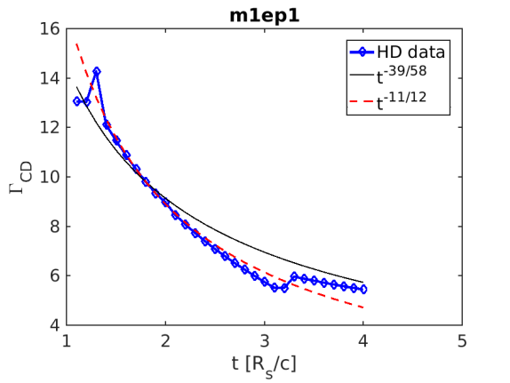
4.2.2 Magnetized secondary wind

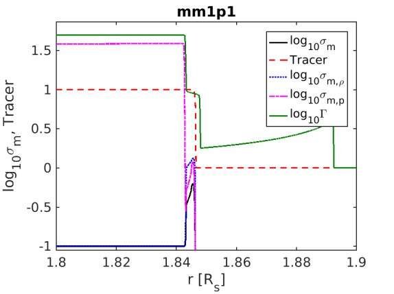
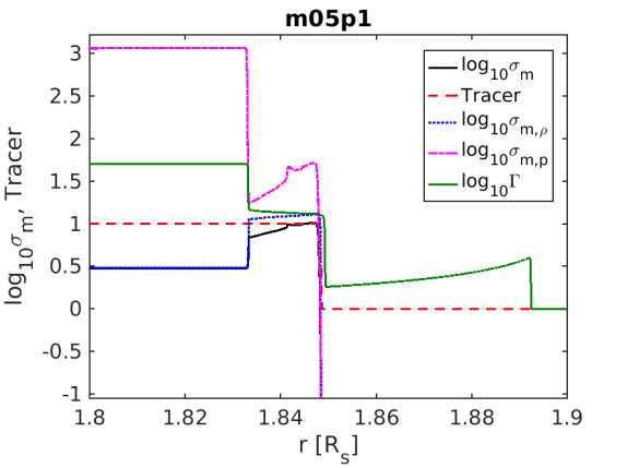
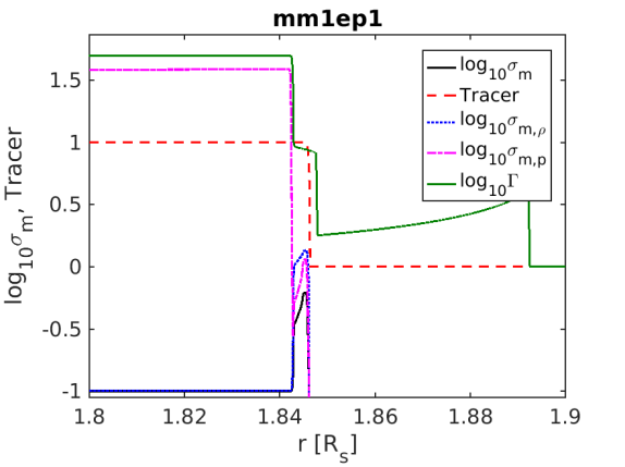
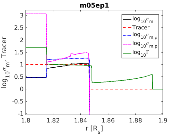
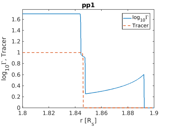
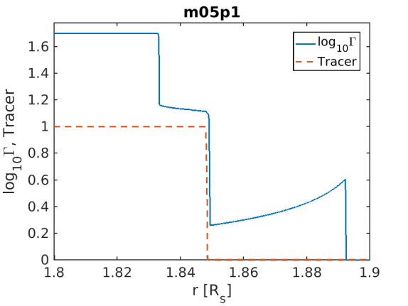
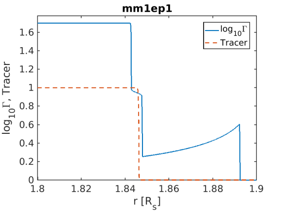
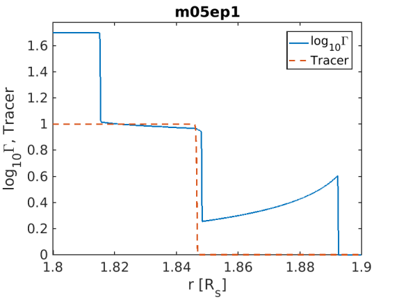
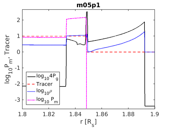
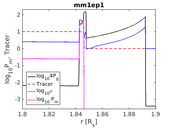
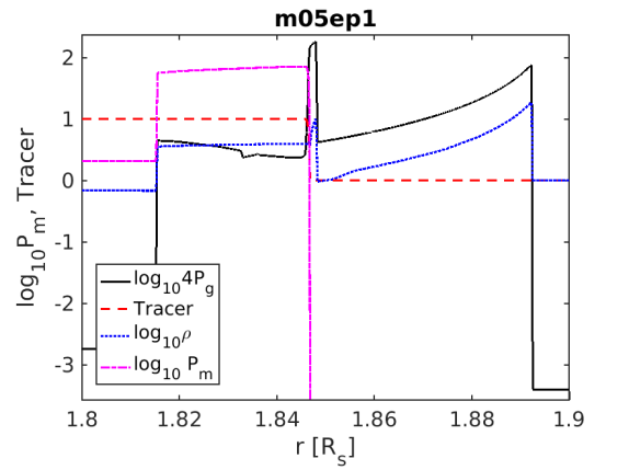
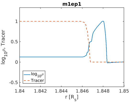
Magnetized models marked as mXXp1 have constant wind density, where XX indicates magnetization of the flow. Magnetized models marked as mXXep1 have constant wind luminosity, where XX indicates magnetization of the flow. As a basis for the magnetized wind models, we choose the model $pp1$, which have $L_{\rm w}r_{\rm s}/c\approx E_{\rm BM}$, so that the total wind power injected during simulation is compatible to the energy of the initial explosion. Figure (9) demonstrates the structure of the solution. The main difference from the unmagnetized models is that the thickness of a layer between FS and RS increases with magnetization, the similar conclusion was obtained by Mimica et al. (2009). This is related to a decrease of compressibility of the magnetized matter. Also note, that in models with similar total power of the wind, the position of FS almost independent of magnetization, while the position of RS strongly depends on the wind magnetization, RS moves slower in highly magnetized models. More solution profiles can be found in the Appendix A.2.

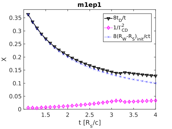
All magnetized wind models show good agreement between theoretical expectation $t_{\rm d}$ and actual ones, see Figure 10. The Lorentz factor of CD is also nicely fitted by theoretical curve eq. (12).

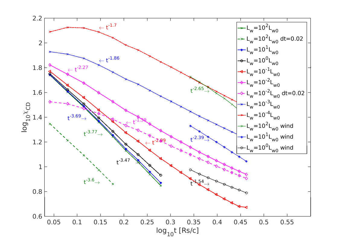
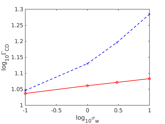
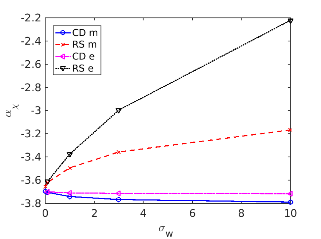
The power of the slope of Lorentz factor of CD is in good agreement with theoretical one for wind independent on its magnetization see Figure 11. Moreover, Lorentz factor of CD very weakly depends on magnetization. If power of the wind is conserved $\Gamma_{\rm CD}\propto\sigma_{\rm w}^{0.023}$, if we preserve hydrodynamical part of the flow and increase magnetization trough increasing magnetic flux, we get $\Gamma_{\rm CD}\propto\sigma_{\rm w}^{0.18}$ that is similar to response of $\Gamma_{\rm CD}$ on increase of wind power.

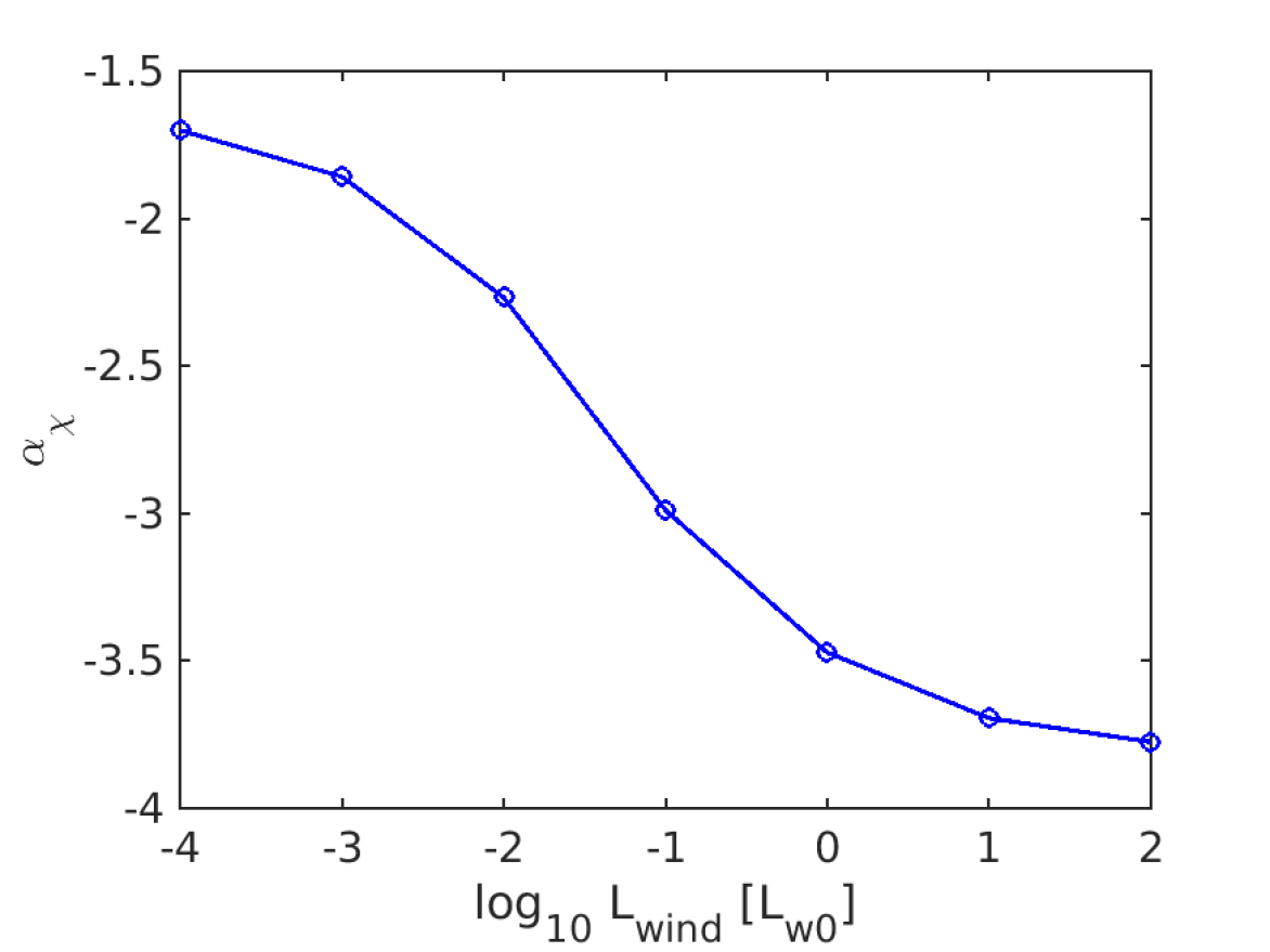
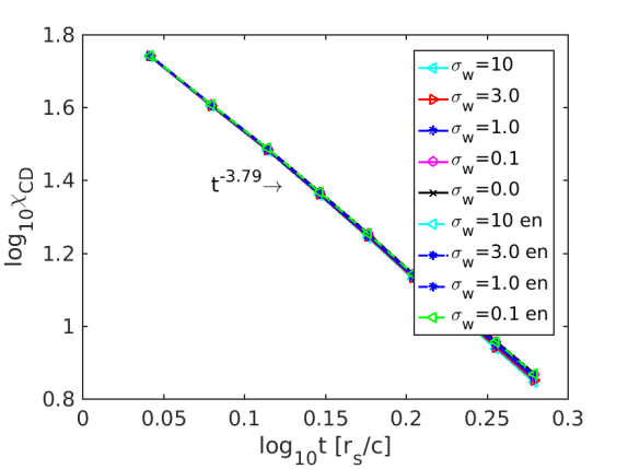
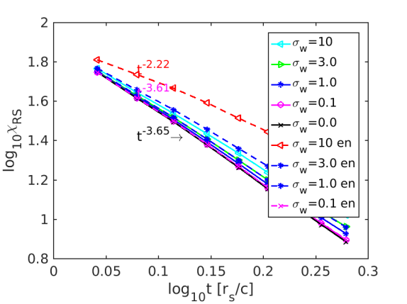
The power slope of time dependents of $\chi_{\rm CD}$, $\alpha_{\rm CD}$ (see Figure 12) almost do not depends on wind magnetization, Figure 13, and its value close to theoretically predicted slope of $-4$.

Figure 9.— Magnetization, tracer and Lorentz factor distribution for magnetized models. As theory predicts, the thickness of reverse shock region increase with magnetization.

Figure 10.— Effects of magnetization on flow dynamics. Top row: self-similar coordinate of the second shock $\chi$ (same as Figure 3) for cases with magnetization $\sigma_{\rm w}=0$ (left) and $\sigma_{\rm w}=10$ (right). Bottom row: Lorentz factor as a function of time – triangles and analytical expectations Lyutikov (2017) for cases with magnetization $\sigma_{\rm w}=0$ (left) and $\sigma_{\rm w}=10$ (right). The jumps in the Lorentz factor at later times occurs when the wind driven FS catches with the leading BMFS.

Figure 11.— Lorentz factor of the contact discontinuity as function of time, left panel, (cf.  Eq. (12) $\Gamma_{\rm CD}\propto t^{-0.92}$). We calculate the power indexes on stright parts of the curves, $0.25<\log_{10}t<0.45$. Dependence of the Lorentz factor of the contact discontinuity on wind magnetization at $t=1.4[R_{\rm s}/c]$, right panel. Red curve is constant total power, blue dashed curve is constant matter power. As expected, in for fixed total power the Lorentz factor of the CD is approximately independent of the the wind magnetization.

Figure 12.— Time dependence of $\chi_{\rm CD}$ (cf.  Eq. (11)) and $\chi_{\rm RS}$ (location of the CD and RS in self-similar coordinate). In a fully self-similar regime the dynamics of the RS follows that of the CD. The low $\sigma$ models do show this property. As we discussed above in the case of the CD, for smaller wind powers the effective time delay $t_{d}$ starts to become important, resulting in smaller temporal indecies. We attribute flatter dependence of $\chi_{\rm CD}$ on time (see also Figure 13) to a somewhat similar effect: for larger $\sigma$ the RS Lorentz factor is smaller, $\propto\Gamma_{\rm CD}/\sqrt{\sigma}$. Thus, beyond some value of $\sigma$ the Lorentz factor of the RS and the correspoding $\chi_{\rm CD}$ are demonstrate flatter temporal profiles.

Figure 13.— Dependence of $\alpha_{\chi}$ on magnetization of the wind ($\chi_{\rm CD}\propto t^{\alpha_{\chi}}$). Diamonds and crosses correspond to contact discontinuity and reverse shock in the case of a preserved energy flux of hydrodynamical flux in the wind. Right triangle and inverted triangle correspond to the case of preserved total energy flux in the wind. (See caption for Figure 12.)

5. Emission from relativistic termination shock: flares, plateaus and steep decays

Next we perform analytical calculations of expected emission properties of highly magnetized RSs. We assume that particles are accelerated at the RS, and then experience radiative and adiabatic decays. In §5.1 we calculate evolution of the distribution function for particle injected at the shock. General relations for the observed intensity are calculated in §5.2.

5.1. Evolution of the distribution function

As discussed above, the dynamics of the second shock depends on the internal structure of the post-first shock flow, and the wind power; all relations are highly complicated by the relativistic and time-of-flight effects. To demonstrate the essential physical effects most clearly, we assume a simplified dynamics of the second shock, allowing it to propagate with constant velocity. Thus, in the frame of the shock, the magnetic field decreases linearly with time,

$$B^{\prime}=B_{0}^{\prime}\frac{t_{0}^{\prime}}{t^{\prime}}$$ (16)

where time $t_{0}^{\prime}$ and magnetic field $B_{0}^{\prime}$ are some constants. In the following, we assume that the RS starts to accelerate particles at time $t_{0}^{\prime}$, and we calculate the emission properties of particles injected at the wind termination shock taking into account radiative and adiabatic losses.

As the wind generated by the long-lasting engine starts to interact with the tail part of the flow generated by the initial explosion, the RS forms in the wind, see Figure 1. Let’s assume that the RS accelerates particles with a power-law distribution,

$$f\left(\gamma^{\prime},t_{i}^{\prime}\right)\propto{\gamma^{\prime}}^{-p}\Theta(\gamma^{\prime}-\gamma_{\text{min}}^{\prime})$$ (17)

where $t_{i}^{\prime}$ is the injection time, $\Theta$ is the step-function, $\gamma^{\prime}$ is the Lorentz factor of the particles, and $\gamma_{\text{min}}^{\prime}$ is the minimum Lorentz factor of the injected particles; primed quantities are measured in the flow frame. The minimal Lorentz factor  $\gamma_{\text{min}}^{\prime}$ can be estimated as (Kennel & Coroniti, 1984b)

$$\gamma_{\text{min}}^{\prime}\sim\gamma_{RS}\sim\gamma_{w}/2\Gamma_{RS}$$ (18)

(We stress that in the pulsar-wind paradigm the minimal Lorentz factor of accelerated particles $\gamma_{\text{min}}^{\prime}$ scales differently from the matter-dominated fireball case, where it is related to a fraction of baryonic energy $\epsilon_{e}$ carried by the wind, e.g. Sari et al., 1998)

The accelerated particles produce synchrotron emission in the ever-decreasing magnetic field, while also experiencing adiabatic losses. Synchrotron losses are given by the standard relations (e.g. Lang, 1999). To take account of adiabatic losses we note that in a toroidally-dominated case the conservation of the first adiabatic invariant (constant magnetic flux through the cyclotron orbit) gives

$$\partial_{t^{\prime}}\ln\gamma^{\prime}=\frac{1}{2}\partial_{t^{\prime}}\ln B^{\prime}$$ (19)

(thus, we assume that that magnetic field is dominated by the large-scale toroidal field).

Using Eqn. (16) for the evolution of the field, the evolution of a particles’ Lorentz factor follows

$$\frac{{d}\gamma^{\prime}}{{dt^{\prime}}}=-\frac{\tilde{C}_{1}{B_{0}^{\prime}}^{2}{\gamma^{\prime}}^{2}}{{t^{\prime}}^{2}}-\frac{\gamma^{\prime}}{2t^{\prime}}\mbox{}$$

$$\tilde{C}_{1}=\frac{\sigma_{T}{t_{0}^{\prime}}^{2}}{6{\pi m_{e}c}}$$ (20)

where $\sigma_{T}$ is the Thomson cross-section and $t_{0}^{\prime}$ is some reference time.

Solving for the evolution of the particles’ energy in the flow frame,

$$\frac{1}{\gamma^{\prime}}=\frac{2\tilde{C}_{1}{B_{0}^{\prime}}^{2}}{3t^{\prime}}\left(\left(\frac{t^{\prime}}{{t}_{i}^{\prime}}\right)^{3/2}-1\right)+\frac{1}{\gamma_{i}^{\prime}}\sqrt{\frac{t^{\prime}}{t_{i}^{\prime}}},$$ (21)

we can derive the evolution of a distribution function (the Green’s function) (e.g. Kardashev, 1962; Kennel & Coroniti, 1984b)

$$G(\gamma^{\prime},t^{\prime},t_{i}^{\prime})=\left\{\begin{array}[]{cc}{\gamma^{\prime}}^{-p}\left(\frac{t_{i}^{\prime}}{t^{\prime}}\right)^{\frac{p-1}{2}}\left(1-\frac{2}{3}\tilde{C}_{1}{B_{0}^{\prime}}^{2}\gamma_{w}^{\prime}\sqrt{t^{\prime}}\left(\frac{1}{{t_{i}^{\prime}}^{3/2}}-\frac{1}{{t^{\prime}}^{3/2}}\right)\right)^{p-2},&{\gamma_{\text{low}}^{\prime}<\gamma^{\prime}<\gamma_{\text{up}}^{\prime}}\\ 0,&{else}\\ \end{array}\right.\mbox{}$$ (24)

$$\frac{1}{\gamma_{\text{low}}^{\prime}}=\frac{2\tilde{C}_{1}{B_{0}^{\prime}}^{2}}{3t^{\prime}}\left(\left(\frac{t^{\prime}}{t_{i}^{\prime}}\right)^{3/2}-1\right)+\frac{1}{\gamma_{min}^{\prime}}\sqrt{\frac{t^{\prime}}{t_{i}^{\prime}}}\mbox{}$$

$$\frac{1}{\gamma_{\text{up}}^{\prime}}=\frac{2\tilde{C}_{1}{B_{0}^{\prime}}^{2}}{3t^{\prime}}\left(\left(\frac{t^{\prime}}{t_{i}^{\prime}}\right)^{3/2}-1\right)$$ (25)

where $\gamma_{\text{low}}^{\prime}$ is a lower bound of Lorentz factor due to minimum Lorentz factor at injection and $\gamma_{\text{up}}^{\prime}$ is an upper bound of Lorentz factor due to cooling.

Once we know the evolution of the distribution function injected at time $t_{i}^{\prime}$, we can use the Green’s function to derive the total distribution function by integrating over the injection times

$${N}(\gamma^{\prime},t^{\prime})\propto\int_{t_{i}^{\prime}}^{t^{\prime}}\dot{n}(t_{i}^{\prime})G(\gamma^{\prime},t^{\prime},t_{i}^{\prime})dt_{i}^{\prime}$$ (26)

where $\dot{n}(t_{i}^{\prime})$ is the injection rate (assumed to the constant below).

5.2. Observed intensity

The intensity observed at each moment depends on the intrinsic luminosity, the geometry of the flow, relativistic, and time-of-flight effects (e.g. Fenimore et al., 1996; Nakar et al., 2003; Piran, 2004).

The intrinsic emissivity at time $t^{\prime}$ depends on the distribution function $N$ and synchrotron power $P_{\omega}$:

$$L^{\prime}(\omega^{\prime},t^{\prime})=\int\int{N_{A}(\gamma^{\prime},t^{\prime})P_{\omega}(\omega^{\prime})}\,d\gamma^{\prime}dA^{\prime}$$ (27)

where $N_{A}$, the number of particles per unit area, is defined as $N_{A}=N/A=N/(2\pi{r^{\prime}}^{2}(1-\cos\theta_{j}))$, $P(\omega^{\prime})$ is the power per unit frequency emitted by each electron, and $dA^{\prime}$ is the surface differential (unlike Fenimore et al., 1996, we do not have extra $\cos\theta$ in the expression for the area since we use volumetric emissivity, not emissivity from a surface).

We assume that the observer is located on the symmetry axis and that the active part of the RS occupies angle $\theta_{j}$ to the line of sight. The emitted power is then

$$L^{\prime}(\omega^{\prime},t^{\prime})=\int_{0}^{\theta_{j}}\int_{\gamma_{\min}^{\prime}}^{\infty}N_{A}(\gamma^{\prime},t^{\prime})P(\omega^{\prime})d\gamma^{\prime}2\pi{r^{\prime}}^{2}\sin(\theta)d\theta$$ (28)

Photons seen by a distant observer at times $T_{ob}$ are emitted at different radii and angles $\theta$. To take account of the time of flight effects, we note that the distance between the initial explosion point and an emission point $(r^{\prime},\theta)$ is $r^{\prime}=vt^{\prime}=vT_{ob}(1-\beta\cos(\theta))^{-1}\gamma_{RS}^{-1}$, where $T_{ob}$ is the observed time. Supposed that a photon was emitted from the distance $r^{\prime}$ and angle $\theta=0$ at time $t^{\prime}$, and at the same time, the other photon was emitted from the distance $r^{\prime}$ and any arbitrary angle $\theta=\theta_{i}<\theta_{j}$. These two photons will be observed at time $T_{0}$ and $T_{\theta_{i}}$, then the relation between $T_{0}$ and $T_{\theta_{i}}$ is given by:

$$r^{\prime}=vt^{\prime}=\frac{vT_{0}}{(1-\beta)\gamma_{RS}}=\frac{vT_{\theta_{i}}}{(1-\beta\cos(\theta_{i}))\gamma_{RS}}$$ (29)

where, the time $t^{\prime}$ measured in the fluid frame, and the corresponding observe time $T_{ob}$, is a function of $\theta$ and $t^{\prime}$:

$$T_{ob}=t\left(1-\beta\cos\theta\right)=t^{\prime}\left(1-\beta\cos\theta\right)\gamma_{RS}$$ (30)

Taking the derivative of Eqn. (30) we find

$$\sin(\theta)d\theta=-\frac{T_{\text{ob}}}{{t^{\prime}}^{2}\beta\gamma_{RS}}dt^{\prime}\approx-\frac{T_{\text{ob}}}{{t^{\prime}}^{2}\gamma_{RS}}dt^{\prime}$$ (31)

Substitute the relation (31) into (28), the observed luminosity becomes

$$L^{\prime}(T_{ob},\omega^{\prime})\approx\int_{t_{\theta^{\prime}=0}^{\prime}}^{t_{\theta^{\prime}=\theta_{j}}^{\prime}}\int_{\gamma_{\min}^{\prime}}^{\infty}\frac{2\pi c^{2}T_{ob}}{\gamma_{RS}}\times N_{A}(\gamma^{\prime},t^{\prime})P(\omega^{\prime})d\gamma^{\prime}dt^{\prime}$$ (32)

To understand the Eqn. (32), the radiation observed at $T_{ob}$ corresponds to the emission angle from $0$ to $\theta_{j}$, which also corresponds to the emission time $t_{\theta^{\prime}=0}^{\prime}={T_{ob}}/{(1-\beta)\gamma_{RS}}$ to $t_{\theta^{\prime}=\theta_{j}}^{\prime}={T_{ob}}/{(1-\beta\cos\theta_{j})\gamma_{RS}}$. So we need to integrate the emissivity function over the range of the emission angle, or integrate the emissivity function over the range of the emission time from $t_{\theta^{\prime}=0}^{\prime}={T_{ob}}/{(1-\beta)\gamma_{RS}}$ to $t_{\theta^{\prime}=\theta_{j}}^{\prime}={T_{ob}}/{(1-\beta\cos\theta_{j})\gamma_{RS}}$.

Finally, taking into account Doppler effects (Doppler shift $\omega=\delta\omega^{\prime}$ and the intensity boost $I_{\omega}\left(\omega\right)=\delta^{3}I_{\omega^{\prime}}^{\prime}\left(\omega^{\prime}\right)$; where $\delta$ is the Doppler factor $\delta=1/({\gamma_{RS}\left(1-\beta\cos\theta\right)})$), substitute the relation $t^{\prime}={T_{\text{ob}}}/{(1-\beta\cos(\theta))\gamma_{RS}}$ into Eqn.(32) we finally arrive at the equation for the observed spectral luminosity:

$$F_{\omega}=\int_{\frac{T_{\text{ob}}}{(1-\beta\cos(\theta_{j}))\gamma_{RS}}}^{\frac{T_{\text{ob}}}{(1-\beta)\gamma_{RS}}}\int_{\gamma_{\min}^{\prime}}^{\infty}\frac{1}{2\gamma_{RS}}c^{2}D^{-2}T_{\text{ob}}\delta^{3}N_{A}P(\omega/\delta)d\gamma^{\prime}dt^{\prime}$$ (33)

where $D$ is the distance to the GRB.

Next we apply these general relations to three specific problem: (i) origin of plateaus in afterglow light curves; (ii) sudden drops in the afterglow light curves §5.3; (iii) afterglow flares, §5.4. For numerical estimates, we assume the redshift $z=1$, the Lorentz factor of the wind $\gamma_{w}=5\times 10^{5}$, the wind luminosity $L_{w}=10^{46}$ erg/s, the initial injection time $t_{0}^{\prime}=10^{5}$s (in jet frame), the power law index of particle distribution $p=2.2$, and the viewing angle is 0 (observer on the axis) for all calculations.

5.3. Results: plateaus and sudden intensity drops in afterglow light curves

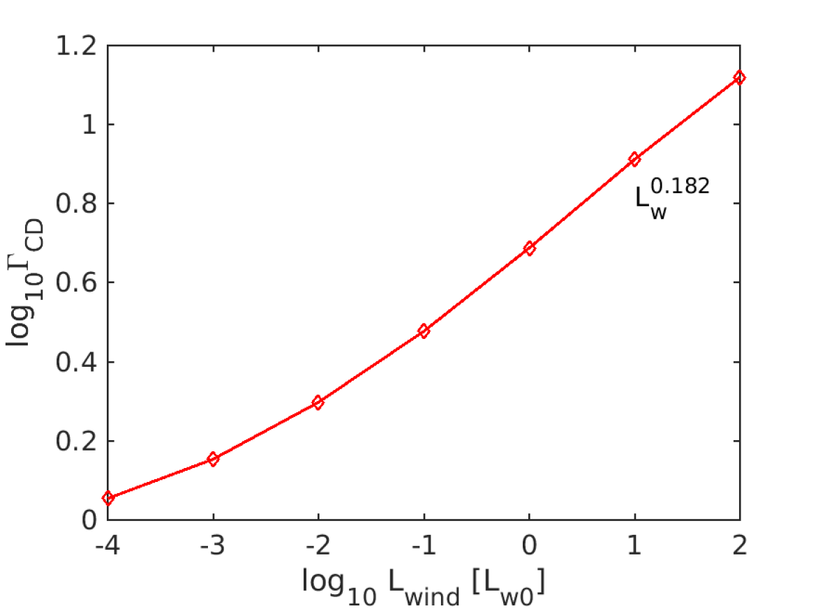
Particles accelerated at the RS emit in the fast cooling regime. The resulting synchrotron luminosity $L_{s}$ is approximately proportional to the wind luminosity $L_{w}$, as discussed by Lyutikov & Camilo Jaramillo (2017). (For highly magnetized winds with $\sigma\gg 1$ the RS emissivity is only mildly suppressed, by high magnetization, $\propto 1/\sqrt{\sigma}$, due to the fact that higher sigma shocks propagate faster with respect to the wind.) Thus, the constant wind will produce a nearly constant light curve: plateaus are natural consequences in our model in the case of constant long-lasting wind, see Figure 14. At the early times all light curves show a nearly constant evolution with time, a plateau, with flux $\propto t_{ob}^{-0.1}$. A slight temporal decrease is due to the fact that magnetic field at the RS decreases with time so that particles emit less efficiently. This observed temporal decrease is flatter than what is typically observed, $\propto t_{ob}^{-\alpha_{2}}$ with $\alpha_{2}=0.5-1$ (Nousek et al., 2006). A steeper decrease can be easily accommodated due to the decreasing wind power. This explains the plateaus.

Figure 14.— The light curve at 100 KeV for different Lorentz factors of the post-RS flow and different jet angles $2/\gamma_{RS}$ (dotted) $1/\gamma_{RS}$ (solid) and $1/(2\gamma_{RS})$ (dot dashed) and different Lorentz factors of the RS. For $\theta_{j}\leq 1/\gamma_{RS}$ the drop in intensity is extremely fast.

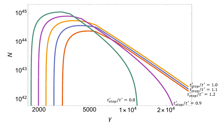
Next we assume that the central engine suddenly stops operating. This process could be due to the collapse of a neutron star into a black hole or sudden depletion of an accretion disk. At a later time, when the “tail” of the wind reaches the termination shock, acceleration stops. Let the injection terminate at a some time $t_{\text{stop}}^{\prime}$. The distribution function in the shocked part of the wind then become

$${N}(\gamma^{\prime},t^{\prime})\propto\int_{t_{0}^{\prime}}^{\min(t^{\prime},t_{\text{stop}}^{\prime})}G(\gamma^{\prime},t^{\prime},t_{i}^{\prime})dt_{i}^{\prime}$$ (34)

Figure 15 shows the evolution of the distribution function by assuming the Lorentz factor of RS $\gamma_{RS}=90$, and the injection is stopped at time $t_{\text{stop}}^{\prime}=1.5\times 10^{5}$s (in this case, the $T_{\text{ob,stop}}=833$s in the observer’s frame). The number of high energy particles drops sharply right after the injection is stopped: particles lose their energy via synchrotron radiation and adiabatic expansion in fast cooling regime.

Figure 15.— Evolution of the distribution function. Here we take account the effect of radiation loss and adiabatic expansion. In our calculation, the Lorentz factor of RS $\gamma_{RS}=90$, and the injection is stopped at time $t_{\text{stop}}^{\prime}=1.5\times 10^{5}$s, $\gamma_{\min}=\gamma_{w}/\gamma_{RS}=5.5\times 10^{3}$, initial magnetic field $B_{0}=2.1$G. The times are measured in fluid frame at $t_{\text{stop}}^{\prime}/t^{\prime}=1.2,1.1,1.0,0.9,0.8$ from red to green curves.

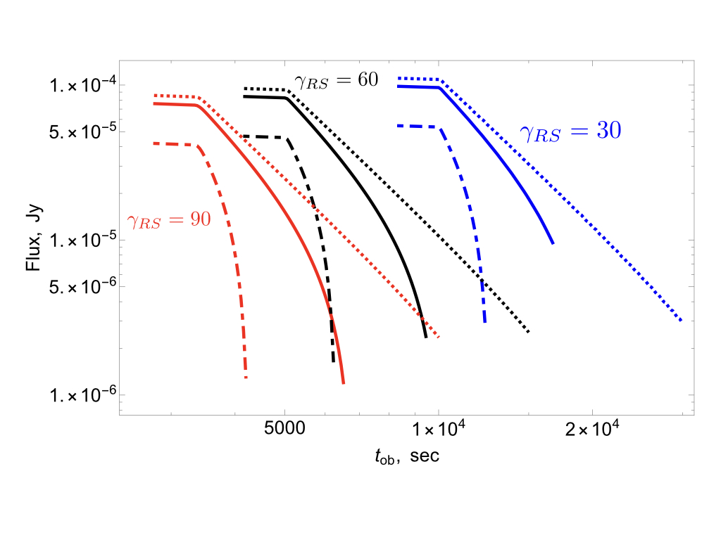
The resulting light curves are plotted in Figure 14. We assume post-RS flow $\gamma_{RS}=30,\,60,\,90$ and three jet opening angles of $\sim(1/2,\,1,\,2)\times\gamma_{RS}^{-1}$. These particular choices of $\theta_{j}$ are motivated by our expectation that sudden switch-off of the acceleration at the RS will lead to fast decays in the observed flux (in the fast cooling regime).

The injection is stopped at a fixed time in the fluid frame, corresponding to $t_{0}^{\prime}=6\times 10^{5}$s. There is a sudden drop of intensity when the injection is stopped ($T_{\text{ob}}=10000$s for blue curve, $T_{\text{ob}}=5000$s for black curve, and $T_{\text{ob}}=3\times 10^{3}$s for red curve). Blue curve has $\gamma_{RS}=30$, $\gamma_{\min}=\gamma_{\text{w}}/\gamma_{RS}=1.65.\times 10^{4}$, initial magnetic field $B_{0}$ = 6.4G; green curve has $\gamma_{RS}=60$, $\gamma_{\min}=\gamma_{w}/\gamma_{RS}=8.3\times 10^{3}$, initial magnetic field $B_{0}$=3.2G; red curve has $\gamma_{RS}=90$, $\gamma_{\min}=\gamma_{w}/\gamma_{RS}=5.5\times 10^{3}$, initial magnetic field $B_{0}$ = 2.1G. Here we assume $B_{0}\propto{\gamma_{RS}}^{-1}$ for our calculations. Smaller jet angle produce sharper drop.

In the simplest qualitative explanation, consider a shell of radius $r_{em}$ extending to a finite angle $\theta_{j}$ and producing an instantaneous flash of emission (instantaneous is an approximation to the fast cooling regime). The observed light curve is then Fenimore et al. (1996)

$$\propto\left\{\begin{array}[]{cc}\left(\frac{T_{ob}}{T_{0}}\right)^{-(\alpha+2)},&0<T_{ob}<\frac{r_{em}/c}{2}\theta_{j}^{2}\\ 0&\frac{r_{em}/c}{2}\theta_{j}^{2}<T_{ob}\end{array}\right.$$ (35)

where $T_{0}=\frac{r_{em}/c}{2\gamma_{RS}^{2}}$ and $\alpha$ is the spectral index. Thus, for $\theta_{j}>1/\gamma_{RS}$ the observed duration of a pulse is $\sim T_{0}$, while for $\theta_{j}<1/\gamma_{RS}$ the pulse lasts much shorter, $\sim T_{0}(\theta_{j}\gamma_{RS})^{2}\ll T_{0}$. Thus, in this case a drop in intensity is faster than what would be expected in either faster shocks or shocks producing emission in slowly cooling regime.

5.4. Results: afterglow flares

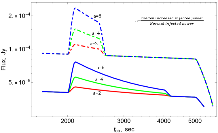
Next, we investigate the possibility that afterglow flares are produced due to the variations in wind power. We re-consider the case of $\gamma_{RS}=60$ (the green curve in Figure 14), but set the ejected power at two, four, and eight times larger than the average power for a short period of time from $2.4\times 10^{5}$s to $2.5\times 10^{5}$s. We consider the two cases: the wide jet angle ($\theta_{j}=1/\gamma_{RS}$) and the narrow jet angle ($\theta_{j}=1/2\gamma_{RS}$). The corresponding light curves are plotted in Figure 16.

Light curves show a sharp rise around $T_{ob}=2000$ corresponding to the increased ejected power $t=2.4\times 10^{5}$s at emission angle $\theta=0$, followed by a sharp drop around $T_{ob}=4000$s for the case of wide jet and $T_{ob}=2500$s for the case of narrow jet (which corresponds to the ending time of the increased ejected power $t=2.5\times 10^{5}$s at emission angle $\theta=\theta_{j}$). Bright flares are clearly seen. Importantly, the corresponding total injected energy is only $\sim 1\%,\,5\%$ and $10\%$ larger than the averaged value. The magnitude of the rise in flux is less than the magnitude of the rise in ejected power (e.g. the rise in ejected power by a factor eight only gives the rise in flux by a factor two), due to the fact that the emission from the increased ejected power from different angles is spread out in observer time. Thus, variations in the wind power, with minor total energy input, can produce bright afterglow flares. (Lyutikov, 2006a)

Figure 16.— Afterglow flares due to variations in wind luminosity for the case $\gamma_{RS}=60$ (green curve in the Figure 14). The ejected power is increased by factors $a=2,4,8$ for a short period from $2.4\times 10^{5}$s to $2.5\times 10^{5}$s (in the fluid frame). Solid lines are for $\theta_{j}=\gamma_{RS}$, dashed lines are for $\theta_{j}=1/2\gamma_{RS}$. For clarity, the relative shift of intensities between the plots for two opening angles is due to our parametrization of the injected power (constant total power not isotropic equivalent).

6. Discussion

In this paper we discuss properties of GRB afterglows within the “pulsar wind” paradigm: long-lasting, ultra-relativistic, highly magnetized wind with particles accelerated at the wind termination shock (Kennel & Coroniti, 1984b). The present model of long lasting winds in GRBs is qualitatively different from previous models based on “fireball” paradigm, see §2.

We first performed a set of detailed RMHD simulations of relativistic double explosions. Our numerical results are in excellent agreement with theoretical prediction (Lyutikov, 2017; Lyutikov & Camilo Jaramillo, 2017). For example, for sufficiently high wind power we have $\Gamma_{\rm CD}\propto t^{-11/12}$, while after $t_{eq}$ the shocks merge and move as a single self-similar shock with $\Gamma_{\rm CD}\propto t^{-1/2}$. In addition numerics demonstrates a much richer set of phenomena (e.g., transitions between various analytical limits and variations in the temporal slopes). We find that even for the case of constant external density and constant wind power the dynamics of the wind termination shock shows a large variety - both in temporal slopes of the scaling of the Lorentz factor of the shock, and producing non-monotonic behavior. Non-self-similar evolution of the wind termination shock occurs for two different reasons: (i) at early times due to a delay in the activation of the long-lasting fast wind; (ii) at late times when the energy injected by the wind becomes comparable to the energy of the initial explosion.

Second, we performed radiative calculations of the RS emission and we demonstrated that emission from the long-lasting relativistic wind can resolve a number of contradicting GRB observations. We can reproduce:

• Afterglow plateaus: in the fast cooling regime the emitted power is comparable to the wind power. Hence, only mild wind luminosity $L_{w}\sim 10^{46}$ erg s^-1 is required (isotropic equivalent)

• Sudden drops in afterglow light curves: if the central engine stops operating, and if at the corresponding moment the Lorentz factor of the RS is of the order of the jet angle, a sudden drop in intensity will be observed.

• Afterglow flares: if the wind intensity varies, this leads to the sharp variations of afterglow luminosities. Importantly, a total injected energy is small compared to the total energy of the explosion.

Lyutikov & Camilo Jaramillo (2017) also discussed how the model provides explanations for a number of other GRB phenomena, like “Naked GRBs problem” (Page et al., 2006; Vetere et al., 2008) (if the explosion does not produce a long-lasting wind, then there will be no X-ray afterglow since RS reflects the properties of wind), “Missing orphan afterglows”: both prompt emission and afterglow emission arise from the engine-powered flow, so they may have similar collimation properties. The model also offers explanations to missing and/or chromatic jet breaks, orphan afterglows, “Missing” reverse shocks (they are not missing - they are dominant).

In conclusion, the high energy emission from highly relativistic wind is (i) highly efficient; (ii) can be smooth (over a period of time) for constant wind parameters; (iii) can react quickly to the changes of the wind properties. RS also contributes to the optical - this explains correlated X-optical features often seen in afterglows. FS emission occurs in the optical range, and, at later times, in radio (Lyutikov & Camilo Jaramillo, 2017).

Appendix A Simulation profiles

A.1. Non magnetized cases

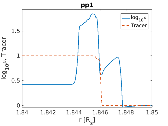
As we can see on the Figure (17) from pm2 to pp2 model, with increasing wind power, the Lorentz factor of FS and RS are also increase while the distance between these shocks becomes smaller, where positions of the shocks are indicated by jumps of pressure; jump of density at constant pressure identifies the CD. Shift of the wind injection radius (compare models $pm2$ and $pm2s$ or $pp2$ and $pp2s$) do not change structure of the solution significantly. Change of injection radius shift position of shocked wind structure as a whole. High resolution of our setup allows to resolve structures of density distribution on the radial scale $\sim 10^{-4}\;r_{\rm s}$ (see Figure 18).

Figure 17.— Gas pressure (thick solid lines), density (dotted line) and tracer (dashed line) as functions of radius at the moment $t=1.9\;[r_{s}/c]$.

Figure 18.— Zoom-in to the region close to the CD: Density (solid line) and tracer (dashed line) as functions of radius at the moment $t=1.9\;[r_{s}/c]$.

A.2. Magnetized cases

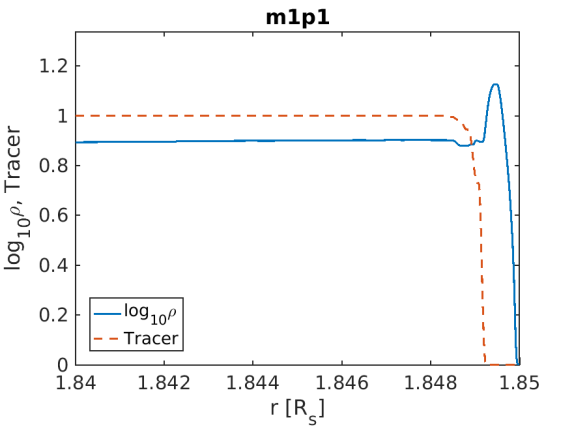
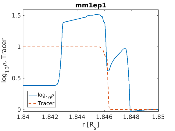
Figures (19), (20) and 21 demonstrate weak dependence of density profile of double shocked matter if the total energy of the wind is preserved. On the other hand, if we are preserving hydrodynamic energy flux in the wind and increases its magnetization, due to increasing of the total power of wind double shocked matter suffer stronger compression and layer double shocked matter became thinner. On other hand increase of magnetization decrease compression ratio of the shocked wind.

Figure 19.— Lorentz factor and tracer distribution as functions of radius at the moment $t=1.9$ for models with different magnetization.

Figure 20.— Gas pressure (thick solid line), density (dotted line) and tracer (dashed line) as functions of radius at the moment $t=1.9$ for models with different magnetization.

Figure 21.— Zoom-in to the regions near the CD. Density (solid line) and tracer (dashed line) as functions of radius at the moment $t=1.9$ for cases with different magnetization.

References

- Barkov & Komissarov (2010) Barkov, M. V., & Komissarov, S. S. 2010, MNRAS, 401, 1644
- Barkov & Pozanenko (2011) Barkov, M. V., & Pozanenko, A. S. 2011, MNRAS, 417, 2161
- Beniamini & Mochkovitch (2017) Beniamini, P., & Mochkovitch, R. 2017, A&A, 605, A60
- Blandford & McKee (1976) Blandford, R. D., & McKee, C. F. 1976, Physics of Fluids, 19, 1130
- Cannizzo & Gehrels (2009) Cannizzo, J. K., & Gehrels, N. 2009, ApJ, 700, 1047
- Chincarini et al. (2010) Chincarini, G., et al. 2010, MNRAS, 406, 2113
- Dai (2004) Dai, Z. G. 2004, ApJ, 606, 1000
- Dai & Lu (1998) Dai, Z. G., & Lu, T. 1998, A&A, 333, L87
- de Pasquale et al. (2007) de Pasquale, M., et al. 2007, MNRAS, 377, 1638
- de Pasquale et al. (2009) —. 2009, MNRAS, 392, 153
- De Pasquale et al. (2016) De Pasquale, M., et al. 2016, MNRAS, 462, 1111
- Fenimore et al. (1996) Fenimore, E. E., Madras, C. D., & Nayakshin, S. 1996, ApJ, 473, 998
- Gat et al. (2013) Gat, I., van Eerten, H., & MacFadyen, A. 2013, ApJ, 773, 2
- Gehrels & Razzaque (2013) Gehrels, N., & Razzaque, S. 2013, Frontiers of Physics, 8, 661
- Genet et al. (2007) Genet, F., Daigne, F., & Mochkovitch, R. 2007, MNRAS, 381, 732
- Gomboc et al. (2009) Gomboc, A., et al. 2009, in American Institute of Physics Conference Series, Vol. 1133, American Institute of Physics Conference Series, ed. C. Meegan, C. Kouveliotou, & N. Gehrels, 145–150
- Hank Childs et al. (2012) Hank Childs, H., Brugger, E., Whitlock, B., & et al. 2012, in High Performance Visualization–Enabling Extreme-Scale Scientific Insight, 357–372
- Hascoët et al. (2017) Hascoët, R., Beloborodov, A. M., Daigne, F., & Mochkovitch, R. 2017, MNRAS, 472, L94
- Ito et al. (2019) Ito, H., Matsumoto, J., Nagataki, S., Warren, D. C., Barkov, M. V., & Yonetoku, D. 2019, Nature Communications, 10, 1504
- Johnson & McKee (1971) Johnson, M. H., & McKee, C. F. 1971, Phys. Rev. D, 3, 858
- Kann et al. (2010) Kann, D. A., et al. 2010, ApJ, 720, 1513
- Kardashev (1962) Kardashev, N. S. 1962, Soviet Ast., 6, 317
- Kargaltsev & Pavlov (2008) Kargaltsev, O., & Pavlov, G. G. 2008, in American Institute of Physics Conference Series, Vol. 983, 40 Years of Pulsars: Millisecond Pulsars, Magnetars and More, ed. C. Bassa, Z. Wang, A. Cumming, & V. M. Kaspi, 171–185
- Kennel & Coroniti (1984a) Kennel, C. F., & Coroniti, F. V. 1984a, ApJ, 283, 694
- Kennel & Coroniti (1984b) —. 1984b, ApJ, 283, 710
- Khangulyan et al. (2020) Khangulyan, D., Aharonian, F., Romoli, C., & Taylor, A. 2020, arXiv e-prints, arXiv:2003.00927
- Khangulyan et al. (2018) Khangulyan, D., Koldoba, A. V., Ustyugova, G. V., Bogovalov, S. V., & Aharonian, F. 2018, ApJ, 860, 59
- Komissarov & Barkov (2007) Komissarov, S. S., & Barkov, M. V. 2007, MNRAS, 382, 1029
- Komissarov & Barkov (2009) —. 2009, MNRAS, 397, 1153
- Krimm et al. (2007a) Krimm, H. A., Boyd, P., Mangano, V., Marshall, F., Sbarufatti, B., & Gehrels, N. 2007a, GRB Coordinates Network, 6014
- Krimm et al. (2007b) Krimm, H. A., et al. 2007b, GCN Report, 26
- Lang (1999) Lang, K. R. 1999, Astrophysical formulae
- Lien et al. (2016) Lien, A., et al. 2016, ApJ, 829, 7
- Lyons et al. (2010) Lyons, N., O’Brien, P. T., Zhang, B., Willingale, R., Troja, E., & Starling, R. L. C. 2010, MNRAS, 402, 705
- Lyutikov (2006a) Lyutikov, M. 2006a, MNRAS, 369, L5
- Lyutikov (2006b) —. 2006b, New Journal of Physics, 8, 119
- Lyutikov (2009) —. 2009, ArXiv e-prints 0911.0349
- Lyutikov (2010) —. 2010, Phys. Rev. E, 82, 056305
- Lyutikov (2011) —. 2011, Phys. Rev. D, 83, 124035
- Lyutikov (2017) —. 2017, Physics of Fluids, 29, 047101
- Lyutikov & Blandford (2003) Lyutikov, M., & Blandford, R. 2003, ArXiv Astrophysics e-prints
- Lyutikov & Camilo Jaramillo (2017) Lyutikov, M., & Camilo Jaramillo, J. 2017, ApJ, 835, 206
- Lyutikov & McKinney (2011) Lyutikov, M., & McKinney, J. C. 2011, Phys. Rev. D, 84, 084019
- Mazaeva et al. (2018) Mazaeva, E., Pozanenko, A., & Minaev, P. 2018, ArXiv e-prints
- Mészáros (2006) Mészáros, P. 2006, Reports on Progress in Physics, 69, 2259
- Mignone et al. (2007) Mignone, A., Bodo, G., Massaglia, S., Matsakos, T., Tesileanu, O., Zanni, C., & Ferrari, A. 2007, ApJS, 170, 228
- Mignone et al. (2009) Mignone, A., Ugliano, M., & Bodo, G. 2009, MNRAS, 393, 1141
- Mimica et al. (2009) Mimica, P., Giannios, D., & Aloy, M. A. 2009, A&A, 494, 879
- Nakar et al. (2003) Nakar, E., Piran, T., & Granot, J. 2003, New. Astr., 8, 495
- Nousek et al. (2006) Nousek, J. A., et al. 2006, ApJ, 642, 389
- Oates et al. (2007) Oates, S. R., et al. 2007, MNRAS, 380, 270
- O’Brien et al. (2006) O’Brien, P. T., et al. 2006, ApJ, 647, 1213
- Oganesyan et al. (2020) Oganesyan, G., Ascenzi, S., Branchesi, M., Salafia, O. S., Dall’Osso, S., & Ghirlanda, G. 2020, ApJ, 893, 88
- Paczynski (1986) Paczynski, B. 1986, ApJ, 308, L43
- Page et al. (2006) Page, K. L., et al. 2006, ApJ, 637, L13
- Panaitescu (2007) Panaitescu, A. 2007, MNRAS, 380, 374
- Panaitescu et al. (2006) Panaitescu, A., Mészáros, P., Gehrels, N., Burrows, D., & Nousek, J. 2006, MNRAS, 366, 1357
- Panaitescu et al. (1998) Panaitescu, A., Mészáros, P., & Rees, M. J. 1998, ApJ, 503, 314
- Piran (1999) Piran, T. 1999, Phys. Rep., 314, 575
- Piran (2004) —. 2004, Reviews of Modern Physics, 76, 1143
- Porth et al. (2014) Porth, O., Komissarov, S. S., & Keppens, R. 2014, MNRAS, 438, 278
- Racusin et al. (2009) Racusin, J. L., et al. 2009, ApJ, 698, 43
- Rees & Meszaros (1992) Rees, M. J., & Meszaros, P. 1992, MNRAS, 258, 41P
- Rees & Meszaros (1994) —. 1994, ApJ, 430, L93
- Rees & Mészáros (1998) Rees, M. J., & Mészáros, P. 1998, ApJ, 496, L1
- Resmi & Zhang (2016) Resmi, L., & Zhang, B. 2016, ApJ, 825, 48
- Rowlinson et al. (2013) Rowlinson, A., O’Brien, P. T., Metzger, B. D., Tanvir, N. R., & Levan, A. J. 2013, MNRAS, 430, 1061
- Rowlinson et al. (2010) Rowlinson, A., et al. 2010, MNRAS, 409, 531
- Sari & Piran (1995) Sari, R., & Piran, T. 1995, ApJ, 455, L143
- Sari & Piran (1999) —. 1999, ApJ, 517, L109
- Sari et al. (1998) Sari, R., Piran, T., & Narayan, R. 1998, ApJ, 497, L17
- Sbarufatti et al. (2007) Sbarufatti, B., Mangano, V., Mineo, T., Cusumano, G., & Krimm, H. 2007, GRB Coordinates Network, 6008
- Sironi & Spitkovsky (2011) Sironi, L., & Spitkovsky, A. 2011, ApJ, 741, 39
- Troja et al. (2007) Troja, E., et al. 2007, ApJ, 665, 599
- Uhm & Beloborodov (2007) Uhm, Z. L., & Beloborodov, A. M. 2007, ApJ, 665, L93
- Uhm et al. (2012) Uhm, Z. L., Zhang, B., Hascoët, R., Daigne, F., Mochkovitch, R., & Park, I. H. 2012, ApJ, 761, 147
- Usov (1992) Usov, V. V. 1992, Nature, 357, 472
- van Eerten (2014) van Eerten, H. 2014, MNRAS, 442, 3495
- Vetere et al. (2008) Vetere, L., Burrows, D. N., Gehrels, N., Meszaros, P., Morris, D. C., & Racusin, J. L. 2008, in American Institute of Physics Conference Series, Vol. 1000, American Institute of Physics Conference Series, ed. M. Galassi, D. Palmer, & E. Fenimore, 191–195
- Warren et al. (2018) Warren, D. C., Barkov, M. V., Ito, H., Nagataki, S., & Laskar, T. 2018, MNRAS, 480, 4060
- Warren et al. (2020) Warren, D. C., Beauchemin, C. A. A., Barkov, M. V., & Nagataki, S. 2020, arXiv e-prints, arXiv:2010.06234
- Warren et al. (2017) Warren, D. C., Ellison, D. C., Barkov, M. V., & Nagataki, S. 2017, ApJ, 835, 248