Applications of the Perturbative Gradient Flow

Fabian Lange^1,2$\star$

15th International Symposium on Radiative Corrections:
Applications of Quantum Field Theory to Phenomenology,
FSU, Tallahasse, FL, USA, 17-21 May 2021 10.21468/SciPostPhysProc.?

Abstract

Over the last decade the gradient flow formalism became an important tool for lattice simulations of Quantum Chromodynamics. It offers remarkable renormalization properties which pave the way for cross-fertilization between perturbative and lattice calculations. In this contribution we discuss the perturbative approach. As first application we compute vacuum expectation values of flowed operators which could help to extract parameters like the strong coupling constant from lattice simulations. Afterwards, we apply the flowed operator product expansion to the time-ordered product of two currents which could be employed for an alternative first-principle evaluation of vacuum polarization functions on the lattice.

 

Contents

1. 1 Introduction
2. 2 Perturbative Gradient Flow
3. 3 Vacuum Expectation Values
4. 4 Flowed Operator Product Expansion
5. 5 Hadronic Vacuum Polarization using Gradient Flow
6. 6 Conclusion

 

1 Introduction

The gradient flow formalism introduced in Refs. [1, 2, 3] became an important tool for simulations of Quantum Chromodynamics (QCD) on the lattice over the last decade. Most prominently, it led to new strategies to set the scale of the lattice, see e.g. Refs. [3, 4, 5]. Moreover, it provides strong renormalization properties. Especially, flowed composite operators constructed from flowed fields do not require renormalization [6]. Therefore, they do not mix under renormalization group (RG) running which allows one to match results of lattice and perturbative calculations without scheme transformation. One prominent application is the extraction of the strong coupling $\alpha_{\mathrm{s}}$ from lattice simulations which, however, did not yield competitive results yet, see Ref. [7] for a recent review.

A powerful tool is the so-called small-flow-time expansion which leads to a relation between flowed and regular operators related by a flow-time dependent mixing matrix [6]. By inverting the mixing matrix, one obtains a flowed operator product expansion (OPE) which expresses the regular operators through the corresponding flowed operators[8, 9, 10]. This was first utilized to construct a regularization independent formula for the energy-momentum tensor (EMT) of QCD [8, 9].

In this contribution we briefly introduce the perturbative treatment of the gradient flow at infinite volume in Section 2 which allows us to compute vacuum expectation values of flowed operators through next-to-next-to-leading order (NNLO) in Section 3. In Section 4, we discuss the flowed OPE and apply it to vacuum polarization functions which might pave the way for an alternative determination of the hadronic corrections to the anomalous magnetic moment and other observables.

2 Perturbative Gradient Flow

The gradient flow formalism continues the gluon and quark fields $A^{a}_{\mu}(x)$ and $\psi(x)$ of regular QCD from $D=4-2\epsilon$ Euclidean dimensions to the fields $B^{a}_{\mu}(t,x)$ and $\chi(t,x$) additionally depending on the flow time $t>0$ through the boundary conditions

$$\begin{split}B_{\mu}^{a}(t=0,x)=A_{\mu}^{a}(x)\,,\qquad\chi(t=0,x)=\psi(x)\end{split}$$ (1)

and the flow equations [3, 12]

$$\partial_{t}B_{\mu}^{a}=\mathcal{D}^{ab}_{\nu}G_{\nu\mu}^{b}+\kappa\mathcal{D}^{ab}_{\mu}\partial_{\nu}B_{\nu}^{b},\qquad\partial_{t}\chi=\Delta\chi-\kappa\partial_{\mu}B_{\mu}^{a}T^{a}\chi,\qquad\partial_{t}\bar{\chi}=\bar{\chi}\overleftarrow{\Delta}+\kappa\bar{\chi}\partial_{\mu}B_{\mu}^{a}T^{a},$$ (2)

where

$$\begin{gathered}G_{\mu\nu}^{a}=\partial_{\mu}B_{\nu}^{a}-\partial_{\nu}B_{\mu}^{a}+f^{abc}B_{\mu}^{b}B_{\nu}^{c},\qquad\mathcal{D}_{\mu}^{ab}=\delta^{ab}\partial_{\mu}-f^{abc}B_{\mu}^{c},\\ \Delta=\mathcal{D}^{\mathrm{F}}_{\mu}\mathcal{D}^{\mathrm{F}}_{\mu},\qquad\overleftarrow{\Delta}=\overleftarrow{\mathcal{D}}^{\mathrm{F}}_{\mu}\overleftarrow{\mathcal{D}}^{\mathrm{F}}_{\mu},\qquad\mathcal{D}^{\mathrm{F}}_{\mu}=\partial_{\mu}+B^{a}_{\mu}T^{a},\qquad\overleftarrow{\mathcal{D}}^{\mathrm{F}}_{\mu}=\overleftarrow{\partial}_{\mu}-B^{a}_{\mu}T^{a}.\end{gathered}$$ (3)

The flow time $t$ is a parameter of mass dimension minus two and we use the short-hand notation $\partial_{t}\equiv\frac{\partial}{\partial t}$. The symmetry generators $T^{a}$ in the fundamental representation and the structure constants $f^{abc}$ are defined through

$$[T^{a},T^{b}]=f^{abc}T^{c},\qquad\mathrm{Tr}(T^{a}T^{b})=-T_{\mathrm{R}}\delta^{ab}.$$ (4)

$\kappa$ is an additional gauge parameter and all physical observables should be independent of it [3]. In perturbative calculations it is usually most convenient to set $\kappa=1$.

The flow equations (2) can be incorporated into a Lagrangian formalism by defining

$$\mathcal{L}=\mathcal{L}_{\mathrm{QCD}}+\mathcal{L}_{\textrm{gauge-fixing}}+\mathcal{L}_{\mathrm{ghost}}+\mathcal{L}_{B}+\mathcal{L}_{\chi}.$$ (5)

The first three terms constituting the regular Yang-Mills Lagrangian are given by

$$\begin{gathered}\mathcal{L}_{\mathrm{QCD}}=\frac{1}{4g_{\mathrm{B}}^{2}}F_{\mu\nu}^{a}F_{\mu\nu}^{a}+\sum_{f=1}^{n_{\mathrm{f}}}\bar{\psi}_{f}(\not{D}^{\mathrm{F}}+m_{f,\mathrm{B}})\psi_{f},\\ \mathcal{L}_{\textrm{gauge-fixing}}=\frac{1}{2g_{\mathrm{B}}^{2}\xi}(\partial_{\mu}A_{\mu}^{a})^{2},\qquad\mathcal{L}_{\mathrm{ghost}}=\frac{1}{g_{\mathrm{B}}^{2}}\partial_{\mu}\bar{c}^{a}D_{\mu}^{ab}c^{b},\end{gathered}$$ (6)

where

$$F_{\mu\nu}^{a}=\partial_{\mu}A^{a}_{\nu}-\partial_{\nu}A^{a}_{\mu}+f^{abc}A_{\mu}^{b}A_{\nu}^{c},\qquad D_{\mu}^{\mathrm{F}}=\partial_{\mu}+A_{\mu}^{a}T^{a},\qquad D_{\mu}^{ab}=\delta^{ab}\partial_{\mu}-f^{abc}A_{\mu}^{c}.$$ (7)

The flow equations are incorporated through

$$\mathcal{L}_{B} =-2\int_{0}^{\infty}\mathrm{d}t\,\textrm{Tr}\left[L_{\mu}^{a}T^{a}\left(\partial_{t}B_{\mu}^{b}T^{b}-\mathcal{D}_{\nu}^{bc}G_{\nu\mu}^{c}T^{b}-\kappa\mathcal{D}_{\mu}^{bc}\partial_{\nu}B_{\nu}^{c}T^{b}\right)\right],$$ (8)

$$\mathcal{L}_{\chi} =\sum_{f=1}^{n_{\mathrm{f}}}\int_{0}^{\infty}\mathrm{d}t\Big{[}\bar{\lambda}_{f}\left(\partial_{t}-\Delta+\kappa\left(\partial_{\mu}B_{\mu}^{a}\right)T^{a}\right)\chi_{f}+\bar{\chi}_{f}\left(\overleftarrow{\partial_{t}}-\overleftarrow{\Delta}-\kappa\left(\partial_{\mu}B_{\mu}^{a}\right)T^{a}\right)\lambda_{f}\Big{]},$$

where $L_{\mu}^{a}(t,x)$, $\lambda_{f}(t,x)$, and $\bar{\lambda}_{f}(t,x)$ are Lagrange multiplier fields [6, 12]. Their Euler-Lagrange equations lead to Eq. 2.

The Feynman rules for perturbative calculations can be derived from the Lagrangian employing standard techniques [6, 12] and the complete list can be found in Ref. [13].

3 Vacuum Expectation Values

VEVs of gauge-invariant operators at finite flow time are among the simplest quantities one can consider within the gradient flow formalism. As mentioned before, these operators do not require any ultra-violet (UV) renormalization beyond that of regular QCD and that of the involved flowed fields [6]. This means that the operators do not mix under RG running, which makes it particularly simple to combine results from different regularization schemes.

The renormalization of the coupling and the masses follows the usual prescription with the known QCD renormalization constants. Throughout this contribution we employ the $\overline{\mathrm{MS}}$ scheme and refer to Refs. [13, 14] for details.

The flowed gauge field $B^{a}_{\mu}(t,x)$ does not require renormalization so that matrix elements of the gluon action density

$$E(t,x)\equiv\tfrac{1}{4}G_{\mu\nu}^{a}(t,x)G_{\mu\nu}^{a}(t,x)$$ (9)

are finite after just the renormalization of $g$ and $m_{f}$ [3, 6]. Hence, a direct comparison of results obtained in different regularization schemes is possible.

In contrast, flowed quark fields require a renormalization factor $Z_{\chi}^{\nicefrac{{1}}{{2}}}(\alpha_{\mathrm{s}})$ in order to render Green’s functions finite. In the $\overline{\mathrm{MS}}$ scheme it reads

$$Z^{-1}_{\chi}(\alpha_{\mathrm{s}})=1-\frac{\alpha_{\mathrm{s}}}{4\pi}\frac{\gamma_{\chi,0}}{\epsilon}+\left(\frac{\alpha_{\mathrm{s}}}{4\pi}\right)^{2}\left[\frac{\gamma_{\chi,0}}{2\epsilon^{2}}\left(\gamma_{\chi,0}+\beta_{0}\right)-\frac{\gamma_{\chi,1}}{2\epsilon}\right]+\mathcal{O}(\alpha_{\mathrm{s}}^{3}),$$ (10)

with

$$\gamma_{\chi,0}=3\,C_{\mathrm{F}},\qquad\gamma_{\chi,1}=\left(\tfrac{223}{6}-8\ln 2\right)C_{\mathrm{A}}C_{\mathrm{F}}-\left(\tfrac{3}{2}+8\ln 2\right)C_{\mathrm{F}}^{2}-\tfrac{22}{3}C_{\mathrm{F}}T_{\mathrm{R}}n_{\mathrm{f}}.$$ (11)

$\gamma_{\chi,0}$ has been computed in Ref. [12], whereas $\gamma_{\chi,1}$ has been obtained by requiring that the NNLO calculations in Refs. [15, 13] become finite.

The scalar quark density

$$S(t,x)\equiv Z_{\chi}\,\sum_{f=1}^{n_{\mathrm{f}}}\bar{\chi}_{f}(t,x)\chi_{f}(t,x)$$ (12)

thus acquires an anomalous dimension, which prevents a direct comparison of results from different regularization schemes. This can be cured by working with ringed quark fields [9], which amounts to renormalizing the flowed quark fields with

$$\mathring{Z}_{\chi}(t,\mu)=-\frac{2N_{\mathrm{C}}n_{\mathrm{f}}}{(4\pi t)^{2}}\cdot\frac{1}{\left.\langle R(t)\rangle\right|_{m=0}}$$ (13)

instead of $Z_{\chi}$, where

$$R(t,x)=\sum_{f=1}^{n_{\mathrm{f}}}\bar{\chi}_{f}(t,x)\overleftrightarrow{\not{\mathcal{D}}}^{\mathrm{F}}\chi_{f}(t,x)\qquad\text{with}\qquad\overleftrightarrow{\mathcal{D}}^{\mathrm{F}}_{\mu}=\mathcal{D}^{\mathrm{F}}_{\mu}-\overleftarrow{\mathcal{D}}^{\mathrm{F}}_{\mu}$$ (14)

is the quark kinetic operator. This corresponds to a “physical” renormalization scheme, which means that the anomalous dimension of the operator

$$\mathring{S}(t,x)=\zeta_{\chi}(t,\mu)\,S(t,x)\qquad\mbox{with}\qquad\zeta_{\chi}(t,\mu)\equiv Z_{\chi}^{-1}\mathring{Z}_{\chi}(t,\mu)$$ (15)

vanishes.

The Feynman rules for the operators $E(t,x)$, $S(t,x)$, and $R(t,x)$ can again be derived by standard techniques and are listed in Ref. [13]. They result in Feynman diagrams like the samples shown in Fig. 1.

(a)

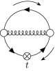
(b)

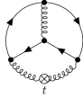
(c)

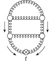
(d)

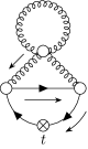
(e)

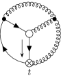
(f)

Figure 1: Sample diagrams for the VEVs through NNLO. Produced with TikZ-Feynman [16].

In Ref. [13] we set up a program chain to automatically generate [17, 18] and process [19, 20, 21, 22, 23] these diagrams as well as to perform a reduction to master integrals [24, 25, 26, 27, 28, 29, 30] and to solve those subsequently [31, 32, 33, 34, 35, 36, 37, 38, 39, 40, 41].

For the gluon action density we then find

$$\begin{gathered}\left.\langle E(t)\rangle\right|_{m=0}=\frac{3\alpha_{\mathrm{s}}}{4\pi t^{2}}\frac{{\rm NewA}}{8}\left[1+\frac{\alpha_{\mathrm{s}}}{4\pi}e_{1}(\mu^{2}t)+\left(\frac{\alpha_{\mathrm{s}}}{4\pi}\right)^{2}e_{2}(\mu^{2}t)+\mathcal{O}(\alpha_{\mathrm{s}}^{3})\right],\\ e_{1}(z)=e_{1,0}+\beta_{0}\,L(z),\qquad e_{2}(z)=e_{2,0}+(2\beta_{0}\,e_{1,0}+\beta_{1})\,L(z)+\beta_{0}^{2}\,L^{2}(z),\end{gathered}$$ (16)

where $\alpha_{\mathrm{s}}=\alpha_{\mathrm{s}}(\mu)$, with $\mu$ the renormalization scale,

$$L(z)\equiv\ln(2z)+\gamma_{\mathrm{E}},$$ (17)

and with the $\overline{\mathrm{MS}}$ coefficients $\beta_{0}$, $\beta_{1}$. For the non-logarithmic coefficients $e_{i,j}$ we find

$$e_{0,0} =1,\qquad e_{1,0}=\big{(}\tfrac{52}{9}+\tfrac{22}{3}\ln 2-3\ln 3\big{)}C_{\mathrm{A}}-\tfrac{8}{9}T_{\mathrm{R}}n_{\mathrm{f}}$$ (18)

$$e_{2,0} =27.9784\,C_{\mathrm{A}}^{2}-(31.5652\ldots)\,C_{\mathrm{A}}T_{\mathrm{R}}n_{\mathrm{f}}+\big{(}16\zeta(3)-\tfrac{43}{3}\big{)}C_{\mathrm{F}}T_{\mathrm{R}}n_{\mathrm{f}}+\big{(}\tfrac{8\pi^{2}}{27}-\tfrac{80}{81}\big{)}T_{\mathrm{R}}^{2}n_{\mathrm{f}}^{2},$$

where $\zeta(3)=1.20206\ldots$. The next-to-leading order (NLO) coefficient $e_{1}$ was first evaluated in Ref. [3] and the NNLO coefficient in Ref. [31]. The three dots in the coefficient of $C_{\mathrm{A}}T_{\mathrm{R}}n_{\mathrm{f}}$ indicate that we were able to obtain the expression in analytical form in Ref. [13]. Our estimate of the numerical accuracy for the $C_{\mathrm{A}}^{2}$ coefficient is at least six digits beyond the four decimal places shown here.

Since these VEVs are formally independent of the renormalization scale $\mu$, the residual scale dependence can be used to study the behavior of the perturbative expansion. As shown in Fig. 2 for $\langle E(t)\rangle$, it is well behaved at high energies and still decent around a central scale of $3$ GeV.

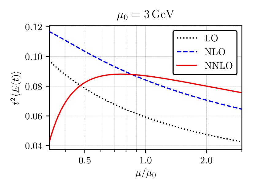
(a)

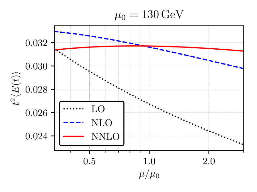
(b)

Figure 2: Renormalization scale dependence of $t^{2}\langle E(t)\rangle$ in QCD for two different central scales $\mu_{0}=e^{-\gamma_{\mathrm{E}}/2}/\sqrt{2t}$. See Ref. [13] for details.

For a detailed discussion and results for $\langle\mathring{S}(t)\rangle$ and $\zeta_{\chi}(t,\mu)$ we refer to Ref. [13].

The proportionality of $\langle E(t)\rangle$ to $\alpha_{\mathrm{s}}$ suggests to define a gradient flow coupling

$$\alpha_{\text{GF}}(t)\equiv\frac{1}{\mathcal{N}}\frac{32\pi}{3{\rm NewA}}t^{2}\langle E(t)\rangle_{\text{lattice}},$$ (19)

based on the determination of $\langle E(t)\rangle_{\text{lattice}}$ through lattice simulations, where $\mathcal{N}$ accounts for boundary conditions [42, 43, 44, 45]. Our perturbative result in Eq. 16 then might help in the extrapolation to infinite volume.

4 Flowed Operator Product Expansion

A powerful concept in the gradient flow formalism is the flowed OPE [8, 9, 10]. Consider a set of operators $\mathcal{O}_{i}(x)$ and a corresponding set of flowed operators $\tilde{\mathcal{O}}_{i}(t,x)$ which are constructed from flowed fields. They are related by the small-flow-time expansion

$$\tilde{\mathcal{O}}_{i}(t,x)=\sum_{j}\zeta_{ij}(t)\mathcal{O}_{j}(x)+O(t)$$ (20)

with the flow-time dependent mixing matrix $\zeta_{ij}(t)$ [6]. By inverting Eq. 20 one can then express any linear combination of the $\mathcal{O}_{i}(x)$ through their flowed counterparts:

$$T=\sum_{i}C_{i}\mathcal{O}_{i}=\sum_{i,j}C_{i}\zeta^{-1}_{ij}\tilde{\mathcal{O}}_{j}+O(t)\equiv\sum_{j}\tilde{C}_{j}\tilde{\mathcal{O}}_{j}+O(t),$$ (21)

where $C_{i}$ are the Wilson coefficients for the object $T$. Since the flowed operators do not require renormalization beyond field and coupling renormalization [6], the r.h.s. is scheme independent. Thus, one can directly relate $T$ in different schemes, for example lattice and perturbative schemes, by employing the flowed OPE. First, it was applied to the EMT [8, 9, 15] which led to promising thermodynamical results [46, 47, 48, 49, 50, 51, 52, 53, 54]. Other applications include charge conjugation parity violating operators for the nucleon electric dipole moment [55] or the electroweak Hamiltonian [56]. We now apply it to vacuum polarization functions (VPFs).

5 Hadronic Vacuum Polarization using Gradient Flow

VPFs for (axial-)vector and (pseudo-)scalar particles are important objects in QCD. Through the optical theorem, their imaginary part is directly related to physical observables such as the decay rates of the $Z$- or the Higgs boson, or the hadronic R-ratio. Moreover, VPFs also contribute indirectly to physical observables such as anomalous magnetic moments [57, 58], the definition of short-distance quark masses [59], or hadronic contributions to the coupling of Quantum Electrodynamics [60, 61]. However, the latter applications involve an integration of the VPFs over the non-perturbative regime. They are typically computed from experimental data with the help of dispersion relations. First-principle lattice calculations have started to become competitive with these dispersive approaches only very recently. However, for the prominent topic of the hadronic vacuum polarization contribution to the muon’s anomalous magnetic moment, the two approaches lead to incompatible results [62].

The perturbative and non-perturbative regimes of VPFs can explicitly be demonstrated through the OPE (see, e.g., Ref. [63]):

$$\begin{split}T(Q)\equiv\int\mathrm{d}^{4}x\,e^{\mathrm{i}Qx}\langle Tj(x)j(0)\rangle\stackrel{{\scriptstyle Q^{2}\to\infty}}{{\sim}}\sum_{k,n}C^{(k),\mathrm{B}}_{n}(Q)\langle\mathcal{O}^{(k)}_{n}(x=0)\rangle,\end{split}$$ (22)

where $j(x)$ generically stands for a scalar, pseudo-scalar, vector, axial-vector, or tensor current, and $k$ labels the mass dimension. In principle, the coefficients $C_{n}^{(k),\mathrm{B}}$ on the r.h.s. of Eq. 22 depend on the quantum numbers of the currents, but we suppress such indices in the following. We furthermore assume that possible global divergences are subtracted off of $T(Q)$.

Up to mass dimension two, only operators proportional to unity contribute to physical matrix elements of QCD. Explicitly, they read

$$\mathcal{O}^{(0)}_{1}\equiv\mathcal{O}^{(0)}=\mathbb{1},\qquad\mathcal{O}^{(2)}_{1}\equiv\mathcal{O}^{(2)}=m_{\mathrm{B}}^{2}\,\mathbb{1},$$ (23)

where $m_{\mathrm{B}}$ is the bare mass of the $n_{\mathrm{h}}$ degenerate massive quarks. Therefore, the Wilson coefficients

$$\begin{split}C_{1}^{(0)}\equiv C^{(0)}\equiv C^{(0),\mathrm{B}},\qquad C_{1}^{(2)}\equiv C^{(2)}\equiv Z_{m}^{2}C^{(2),\mathrm{B}}\end{split}$$ (24)

are UV-finite, where $Z_{m}$ is the $\overline{\mathrm{MS}}$ renormalization constant of the quark mass. At mass dimension four we choose

$$\mathcal{O}^{(4)}_{1}\equiv\mathcal{O}_{1}=\frac{1}{g_{\mathrm{B}}^{2}}F^{a}_{\mu\nu}F^{a}_{\mu\nu},\qquad\mathcal{O}^{(4)}_{2}\equiv\mathcal{O}_{2}=\sum_{f=1}^{n_{\mathrm{f}}}\bar{\psi}_{f}\overleftrightarrow{\not{D}}^{\mathrm{F}}\psi_{f},\qquad\mathcal{O}^{(4)}_{3}\equiv\mathcal{O}_{3}=m_{\mathrm{B}}^{4}\,\mathbb{1}$$ (25)

as basis of operators. Higher dimensional operators are neglected in the following.

Matrix elements of the dimension-four operators are divergent in general. However, by defining renormalized operators $\mathcal{O}_{n}^{\mathrm{R}}$ as linear combinations among them, physical matrix elements as well as the Wilson coefficients become finite, i.e.

$$\begin{split}\mathcal{O}^{\mathrm{R}}_{n}=\sum_{k}Z_{nk}\,\mathcal{O}_{k},\qquad C_{n}=\sum_{m}C^{\mathrm{B}}_{m}(Z^{-1})_{mn},\end{split}$$ (26)

where $C^{\mathrm{B}}_{n}\equiv C_{n}^{(4),\mathrm{B}}$, cf. Eqs. 22 and 25. Since the operators of Eq. 25 are part of the QCD Lagrangian, the renormalization matrix $Z$ can be expressed in terms of the anomalous dimensions of QCD [64, 65].

To derive the flowed OPE, we introduce the flowed operators as

$$\begin{gathered}\tilde{\mathcal{O}}_{1}(t,x)=\frac{Z_{\mathrm{s}}}{g_{\mathrm{B}}^{2}}\,G^{a}_{\mu\nu}(t,x)G^{a}_{\mu\nu}(t,x)=\frac{4}{\hat{\mu}^{2\epsilon}g^{2}}E(t,x),\\ \tilde{\mathcal{O}}_{2}(t,x)=\mathring{Z}_{\chi}\sum_{f=1}^{n_{\mathrm{f}}}\bar{\chi}_{f}(t,x)\overleftrightarrow{\not{\mathcal{D}}}^{\mathrm{F}}(t,x)\chi_{f}(t,x)=\mathring{R}(t,x),\qquad\tilde{\mathcal{O}}_{3}(t,x)=m^{4}\,\mathbb{1},\end{gathered}$$ (27)

where $E(t,x)$ and $\mathring{R}(t,x)$ are the composite operators already introduced in Section 3. The small-flow-time expansion in Eq. 20 allows us to relate the regular QCD operators and coefficients with their flowed counterparts through

$$\tilde{\mathcal{O}}_{n}(t)=\zeta^{(0)}_{n}(t)\mathbb{1}+\zeta^{(2)}_{n}(t)\,m^{2}\mathbb{1}+\sum_{k}\zeta_{nk}(t)\mathcal{O}^{\mathrm{R}}_{k}+O(t),$$ (28)

where $\zeta^{(2)}_{n}(t)$ and $\zeta_{nk}(t)$ are the renormalized, finite mixing coefficients. Inverting Eq. 28 yields

$$\mathcal{O}^{\mathrm{R}}_{n}=\sum_{k}\zeta_{nk}^{-1}(t)\,\bar{\mathcal{O}}_{k}(t)+O(t),\qquad\bar{\mathcal{O}}_{n}(t)\equiv\tilde{\mathcal{O}}_{n}(t)-\zeta^{(0)}_{n}(t)\mathbb{1}-\zeta^{(2)}_{n}(t)m^{2}\mathbb{1},$$ (29)

which leads to the flowed OPE for the current correlator:

$$T(Q)\stackrel{{\scriptstyle Q^{2}\to\infty}}{{\sim}}\tilde{C}^{(0)}(Q^{2},t)+\tilde{C}^{(2)}(Q^{2},t)m^{2}+\sum_{n}\tilde{C}_{n}(Q^{2},t)\langle\tilde{\mathcal{O}}_{n}(t)\rangle+O(t).$$ (30)

The flowed Wilson coefficients are related to the regular Wilson coefficients through

$$\tilde{C}_{n}(Q^{2},t)=\sum_{k}C_{k}(Q^{2})\zeta_{kn}^{-1}(t),\qquad\tilde{C}^{(0,2)}(Q^{2},t)=C^{(0,2)}(Q^{2})-\sum_{n}\tilde{C}_{n}(Q^{2},t)\,\zeta^{(0,2)}_{n}(t).$$ (31)

The regular Wilson coefficients $C^{(0)}$ and $C^{(2)}$ are given by the first two terms in $\nicefrac{{m^{2}}}{{Q^{2}}}$ of the large-$Q^{2}$ expansion of the VPFs. Through the required order, they can be found in Ref. [66] for vector-, in Ref. [67] for axial-vector-, and in Ref. [68] for scalar- and pseudo-scalar currents, for example. The dimension-four coefficients can be found in Refs. [69, 70].

In Ref. [14] we determined the mixing matrix $\zeta$ through NNLO with the help of the method of projectors [71, 72]. Most of the matrix elements can already be extracted from the calculation of the VEVs in Section 3 (or rather Ref. [13]) as well as from the calculation of the EMT in Ref. [15]. The remaining elements correspond to higher-order corrections in the bare mass to the VEVs. By combining $\zeta$ with the known results for the regular Wilson coefficients, one can determine the flowed coefficients of Eq. 31 to the same order. Together with an evaluation of the flowed operator matrix elements on the lattice, the VPFs can be extracted and used in the determination of various physical quantities.

6 Conclusion

In this contribution we discussed the perturbative gradient flow and stressed its powerful renormalization properties. Then, we outlined the calculation of some VEVs of gauge-invariant operators at finite flow time which enable the construction of a gradient flow coupling. Afterwards, we discussed the flowed OPE which can be used to replace regular operators by their better behaved flowed counterparts and applied it to VPFs which might lead to new results for quantities like anomalous magnetic moments from lattice simulations.

References

- [1] R. Narayanan and H. Neuberger, Infinite N phase transitions in continuum Wilson loop operators, JHEP 03, 064 (2006), 10.1088/1126-6708/2006/03/064, hep-th/0601210.
- [2] M. Lüscher, Trivializing Maps, the Wilson Flow and the HMC Algorithm, Commun. Math. Phys. 293, 899 (2010), 10.1007/s00220-009-0953-7, 0907.5491.
- [3] M. Lüscher, Properties and uses of the Wilson flow in lattice QCD, JHEP 08, 071 (2010), 10.1007/JHEP08(2010)071, [Erratum: JHEP 03, 092 (2014)], 1006.4518.
- [4] Sz. Borsányi et al., High-precision scale setting in lattice QCD, JHEP 09, 010 (2012), 10.1007/JHEP09(2012)010, 1203.4469.
- [5] R. Sommer, Scale setting in lattice QCD, PoS LATTICE2013, 015 (2014), 10.22323/1.187.0015, 1401.3270.
- [6] M. Lüscher and P. Weisz, Perturbative analysis of the gradient flow in non-abelian gauge theories, JHEP 02, 051 (2011), 10.1007/JHEP02(2011)051, 1101.0963.
- [7] M. Dalla Brida, Past, present, and future of precision determinations of the QCD coupling from lattice QCD, Eur. Phys. J. A 57, 66 (2021), 10.1140/epja/s10050-021-00381-3, 2012.01232.
- [8] H. Suzuki, Energy–momentum tensor from the Yang–Mills gradient flow, PTEP 2013, 083B03 (2013), 10.1093/ptep/ptt059, [Erratum: PTEP 2015, 079201 (2015)], 1304.0533.
- [9] H. Makino and H. Suzuki, Lattice energy–momentum tensor from the Yang–Mills gradient flow—inclusion of fermion fields, PTEP 2014, 063B02 (2014), 10.1093/ptep/ptu070, [Erratum: PTEP 2015, 079202 (2015), 1403.4772.
- [10] C. Monahan and K. Orginos, Locally smeared operator product expansions in scalar field theory, Phys. Rev. D 91, 074513 (2015), 10.1103/PhysRevD.91.074513, 1501.05348.
- [11] M. Dalla Brida and M. Lüscher, SMD-based numerical stochastic perturbation theory, Eur. Phys. J. C 77, 308 (2017), 10.1140/epjc/s10052-017-4839-0, 1703.04396.
- [12] M. Lüscher, Chiral symmetry and the Yang-Mills gradient flow, JHEP 04, 123 (2013), 10.1007/JHEP04(2013)123, 1302.5246.
- [13] J. Artz, R. V. Harlander, F. Lange, T. Neumann and M. Prausa, Results and techniques for higher order calculations within the gradient-flow formalism, JHEP 06, 121 (2019), 10.1007/JHEP06(2019)121, [Erratum: JHEP 10, 032 (2019)], 1905.00882.
- [14] R. V. Harlander, F. Lange and T. Neumann, Hadronic vacuum polarization using gradient flow, JHEP 08, 109 (2020), 10.1007/JHEP08(2020)109, 2007.01057.
- [15] R. V. Harlander, Y. Kluth and F. Lange, The two-loop energy–momentum tensor within the gradient-flow formalism, Eur. Phys. J. C 78, 944 (2018), 10.1140/epjc/s10052-018-6415-7, [Erratum: Eur. Phys. J. C 79, 858 (2019)], 1808.09837.
- [16] J. P. Ellis, TikZ-Feynman: Feynman diagrams with TikZ, Comput. Phys. Commun. 210, 103 (2017), 10.1016/j.cpc.2016.08.019, 1601.05437.
- [17] P. Nogueira, Automatic Feynman Graph Generation, J. Comput. Phys. 105, 279 (1993), 10.1006/jcph.1993.1074.
- [18] P. Nogueira, Abusing QGRAF, Nucl. Instrum. Methods Phys. Res. 559, 220 (2006), 10.1016/j.nima.2005.11.151.
- [19] R. Harlander, T. Seidensticker and M. Steinhauser, Corrections of to the decay of the Z boson into bottom quarks, Phys. Lett. B 426, 125 (1998), 10.1016/S0370-2693(98)00220-2, hep-ph/9712228.
- [20] T. Seidensticker, Automatic application of successive asymptotic expansions of Feynman diagrams (1999), hep-ph/9905298.
- [21] J. A. M. Vermaseren, New features of FORM (2000), math-ph/0010025.
- [22] J. Kuipers, T. Ueda, J. A. M. Vermaseren and J. Vollinga, FORM version 4.0, Comput. Phys. Commun. 184, 1453 (2013), 10.1016/j.cpc.2012.12.028, 1203.6543.
- [23] T. van Ritbergen, A. N. Schellekens and J. A. M. Vermaseren, Group theory factors for Feynman diagrams, Int. J. Mod. Phys. A 14, 41 (1999), 10.1142/S0217751X99000038, hep-ph/9802376.
- [24] F. V. Tkachov, A theorem on analytical calculability of 4-loop renormalization group functions, Phys. Lett. B 100, 65 (1981), 10.1016/0370-2693(81)90288-4.
- [25] K. G. Chetyrkin and F. V. Tkachov, Integration by parts: The algorithm to calculate -functions in 4 loops, Nucl. Phys. B 192, 159 (1981), 10.1016/0550-3213(81)90199-1.
- [26] S. Laporta, High-precision calculation of multiloop Feynman integrals by difference equations, Int. J. Mod. Phys. A 15, 5087 (2000), 10.1016/S0217-751X(00)00215-7, hep-ph/0102033.
- [27] P. Maierhöfer, J. Usovitsch and P. Uwer, Kira—A Feynman integral reduction program, Comput. Phys. Commun. 230, 99 (2018), 10.1016/j.cpc.2018.04.012, 1705.05610.
- [28] J. Klappert, F. Lange, P. Maierhöfer and J. Usovitsch, Integral reduction with Kira 2.0 and finite field methods, Comput. Phys. Commun. 266, 108024 (2021), 10.1016/j.cpc.2021.108024, 2008.06494.
- [29] J. Klappert and F. Lange, Reconstructing rational functions with FireFly, Comput. Phys. Commun. 247, 106951 (2020), 10.1016/j.cpc.2019.106951, 1904.00009.
- [30] J. Klappert, S. Y. Klein and F. Lange, Interpolation of dense and sparse rational functions and other improvements in FireFly, Comput. Phys. Commun. 264, 107968 (2021), 10.1016/j.cpc.2021.107968, 2004.01463.
- [31] R. V. Harlander and T. Neumann, The perturbative QCD gradient flow to three loops, JHEP 06, 161 (2016), 10.1007/JHEP06(2016)161, 1606.03756.
- [32] T. Binoth and G. Heinrich, An automatized algorithm to compute infrared divergent multi-loop integrals, Nucl. Phys. B 585, 741 (2000), 10.1016/S0550-3213(00)00429-6, hep-ph/0004013.
- [33] T. Binoth and G. Heinrich, Numerical evaluation of multiloop integrals by sector decomposition, Nucl. Phys. B 680, 375 (2004), 10.1016/j.nuclphysb.2003.12.023, hep-ph/0305234.
- [34] A. V. Smirnov and M. N. Tentyukov, Feynman Integral Evaluation by a Sector decomposiTion Approach (FIESTA), Comput. Phys. Commun. 180, 735 (2009), 10.1016/j.cpc.2008.11.006, 0807.4129.
- [35] A. V. Smirnov, V. A. Smirnov and M. Tentyukov, FIESTA 2: Parallelizeable multiloop numerical calculations, Comput. Phys. Commun. 182, 790 (2011), 10.1016/j.cpc.2010.11.025, 0912.0158.
- [36] A. V. Smirnov, FIESTA 3: Cluster-parallelizable multiloop numerical calculations in physical regions, Comput. Phys. Commun. 185, 2090 (2014), 10.1016/j.cpc.2014.03.015, 1312.3186.
- [37] A. C. Genz and A. A. Malik, An Imbedded Family of Fully Symmetric Numerical Integration Rules, SIAM J. Numer. Anal. 20, 580 (1983), 10.1137/0720038.
- [38] Wolfram Research, Inc., Mathematica, Version 11.3, Champaign, IL, 2018.
- [39] T. Huber and D. Maître, HypExp, a Mathematica package for expanding hypergeometric functions around integer-valued parameters, Comput. Phys. Commun. 175, 122 (2006), 10.1016/j.cpc.2006.01.007, hep-ph/0507094.
- [40] T. Huber and D. Maître, HypExp 2, Expanding hypergeometric functions about half-integer parameters, Comput. Phys. Commun. 178, 755 (2008), 10.1016/j.cpc.2007.12.008, 0708.2443.
- [41] E. Panzer, Algorithms for the symbolic integration of hyperlogarithms with applications to Feynman integrals, Comput. Phys. Commun. 188, 148 (2015), 10.1016/j.cpc.2014.10.019, 1403.3385.
- [42] M. Lüscher, Step scaling and the Yang-Mills gradient flow, JHEP 06, 105 (2014), 10.1007/JHEP06(2014)105, 1404.5930.
- [43] Z. Fodor, K. Holland, J. Kuti, D. Nogradi and C. H. Wong, A new method for the beta function in the chiral symmetry broken phase, EPJ Web Conf. 175, 08027 (2018), 10.1051/epjconf/201817508027, 1711.04833.
- [44] A. Hasenfratz and O. Witzel, Continuous renormalization group function from lattice simulations, Phys. Rev. D 101, 034514 (2020), 10.1103/PhysRevD.101.034514, 1910.06408.
- [45] Z. Fodor, K. Holland, J. Kuti, D. Nogradi and C. H. Wong, Case studies of near-conformal -functions, PoS LATTICE2019, 121 (2019), 10.22323/1.363.0121, 1912.07653.
- [46] M. Asakawa, T. Hatsuda, E. Itou, M. Kitazawa and H. Suzuki, Thermodynamics of gauge theory from gradient flow on the lattice, Phys. Rev. D 90, 011501 (2014), 10.1103/PhysRevD.90.011501, [Erratum: Phys. Rev. D 92, 059902 (2015)], 1312.7492.
- [47] Y. Taniguchi, S. Ejiri, R. Iwami, K. Kanaya, M. Kitazawa, H. Suzuki, T. Umeda and N. Wakabayashi, Exploring = 2+1 QCD thermodynamics from the gradient flow, Phys. Rev. D 96, 014509 (2017), 10.1103/PhysRevD.96.014509, [Erratum: Phys. Rev. D 99, 059904 (2019)], 1609.01417.
- [48] M. Kitazawa, T. Iritani, M. Asakawa, T. Hatsuda and H. Suzuki, Equation of state for SU(3) gauge theory via the energy-momentum tensor under gradient glow, Phys. Rev. D 94, 114512 (2016), 10.1103/PhysRevD.94.114512, 1610.07810.
- [49] M. Kitazawa, T. Iritani, M. Asakawa and T. Hatsuda, Correlations of the energy-momentum tensor via gradient flow in SU(3) Yang-Mills theory at finite temperature, Phys. Rev. D 96, 111502 (2017), 10.1103/PhysRevD.96.111502, 1708.01415.
- [50] R. Yanagihara, T. Iritani, M. Kitazawa, M. Asakawa and T. Hatsuda, Distribution of stress tensor around static quark–anti-quark from Yang-Mills gradient flow, Phys. Lett. B 789, 210 (2019), 10.1016/j.physletb.2018.09.067, 1803.05656.
- [51] T. Iritani, M. Kitazawa, H. Suzuki and H. Takaura, Thermodynamics in quenched QCD: energy–momentum tensor with two-loop order coefficients in the gradient-flow formalism, PTEP 2019, 023B02 (2019), 10.1093/ptep/ptz001, 1812.06444.
- [52] M. Kitazawa, S. Mogliacci, I. Kolbé and W. A. Horowitz, Anisotropic pressure induced by finite-size effects in SU(3) Yang-Mills theory, Phys. Rev. D 99, 094507 (2019), 10.1103/PhysRevD.99.094507, 1904.00241.
- [53] Y. Taniguchi, S. Ejiri, K. Kanaya, M. Kitazawa, H. Suzuki and T. Umeda, = 2+1 QCD thermodynamics with gradient flow using two-loop matching coefficients, Phys. Rev. D 102, 014510 (2020), 10.1103/PhysRevD.102.014510, 2005.00251.
- [54] R. Yanagihara, M. Kitazawa, M. Asakawa and T. Hatsuda, Distribution of energy-momentum tensor around a static quark in the deconfined phase of SU() Yang-Mills theory, Phys. Rev. D 102, 114522 (2020), 10.1103/PhysRevD.102.114522, 2010.13465.
- [55] M. D. Rizik, C. J. Monahan and A. Shindler, Short flow-time coefficients of -violating operators, Phys. Rev. D 102, 034509 (2020), 10.1103/PhysRevD.102.034509, 2005.04199.
- [56] A. Suzuki, Y. Taniguchi, H. Suzuki and K. Kanaya, Four quark operators for kaon bag parameter with gradient flow, Phys. Rev. D 102, 034508 (2020), 10.1103/PhysRevD.102.034508, 2006.06999.
- [57] F. Jegerlehner, The Anomalous Magnetic Moment of the Muon, Springer Tracts Mod. Phys. 274 (2017), 10.1007/978-3-319-63577-4.
- [58] T. Aoyama et al., The anomalous magnetic moment of the muon in the Standard Model, Phys. Rep. 887, 1 (2020), 10.1016/j.physrep.2020.07.006, 2006.04822.
- [59] K. G. Chetyrkin, J. H. Kühn, A. Maier, P. Maierhöfer, P. Marquard, M. Steinhauser and C. Sturm, Precise charm- and bottom-quark masses: Theoretical and experimental uncertainties, Theor. Math. Phys. 170, 217 (2012), 10.1007/s11232-012-0024-7, 1010.6157.
- [60] A. Crivellin, M. Hoferichter, C. A. Manzari and M. Montull, Hadronic Vacuum Polarization: versus Global Electroweak Fits, Phys. Rev. Lett. 125, 091801 (2020), 10.1103/PhysRevLett.125.091801, 2003.04886.
- [61] A. Keshavarzi, W. J. Marciano, M. Passera and A. Sirlin, Muon and connection, Phys. Rev. D 102, 033002 (2020), 10.1103/PhysRevD.102.033002, 2006.12666.
- [62] Sz. Borsanyi et al., Leading hadronic contribution to the muon magnetic moment from lattice QCD, Nature 593, 51 (2021), 10.1038/s41586-021-03418-1, 2002.12347.
- [63] C. A. Dominguez, Analytical determination of the QCD quark masses, Int. J. Mod. Phys. A 29, 1430069 (2014), 10.1142/S0217751X14300695, 1411.3462.
- [64] V. P. Spiridonov, Anomalous Dimension of and -function (1984), IYaI-P-0378.
- [65] V. P. Spiridonov and K. G. Chetyrkin, Nonleading mass corrections and renormalization of the operators and , Sov. J. Nucl. Phys. 47, 522 (1988).
- [66] K. G. Chetyrkin, R. Harlander, J. H. Kühn and M. Steinhauser, Mass corrections to the vector current correlator, Nucl. Phys. B 503, 339 (1997), 10.1016/S0550-3213(97)00383-0, hep-ph/9704222.
- [67] R. Harlander and M. Steinhauser, corrections to top quark production at colliders, Eur. Phys. J. C 2, 151 (1998), 10.1007/s100520050129, hep-ph/9710413.
- [68] R. Harlander and M. Steinhauser, Higgs boson decay to top quarks at , Phys. Rev. D 56, 3980 (1997), 10.1103/PhysRevD.56.3980, hep-ph/9704436.
- [69] K. G. Chetyrkin, S. G. Gorishny and V. P. Spiridonov, Wilson expansion for correlators of vector currents at the two-loop level: Dimension-four operators, Phys. Lett. B 160, 149 (1985), 10.1016/0370-2693(85)91482-0.
- [70] R. Harlander, Quarkmasseneffekte in der Quantenchromodynamik und asymptotische Entwicklung von Feynman-Integralen, Ph.D. thesis, Universität Karlsruhe (1998).
- [71] S. G. Gorishny, S. A. Larin and F. V. Tkachov, The algorithm for OPE coefficient functions in the MS scheme, Phys. Lett. B 124, 217 (1983), 10.1016/0370-2693(83)91439-9.
- [72] S. G. Gorishny and S. A. Larin, Coefficient functions of asymptotic operator expansions in minimal subtraction scheme, Nucl. Phys. B 283, 452 (1987), 10.1016/0550-3213(87)90283-5.