\preprintnumber

KYUSHU-HET-140

Lattice energy–momentum tensor from the Yang–Mills gradient flow—inclusion of fermion fields

\name\fnameHiroki \surnameMakino1    \name\fnameHiroshi \surnameSuzuki1 1 hsuzuki@phys.kyushu-u.ac.jp Department of Physics, Kyushu University, 6-10-1 Hakozaki, Higashi-ku, Fukuoka, 812-8581, Japan
Abstract

Local products of fields deformed by the so-called Yang–Mills gradient flow become renormalized composite operators. This fact has been utilized to construct a correctly normalized conserved energy–momentum tensor in the lattice formulation of the pure Yang–Mills theory. In the present paper, this construction is further generalized for vector-like gauge theories containing fermions.

\subjectindex

B01, B31, B32, B38

1 Introduction and the main result

Energy and momentum are fundamental notions in physics. In lattice field theory (the best-developed non-perturbative formulation of quantum field theory), however, the construction of the corresponding Noether current, the energy–momentum tensor Callan:1970ze ; Coleman:1970je ; Freedman:1974gs ; Joglekar:1975jm , is not straightforward Caracciolo:1988hc ; Caracciolo:1989pt , because the translational invariance is explicitly broken by the lattice structure. In a recent paper Suzuki:2013gza , a possible method to avoid this complication being inherent in the energy–momentum tensor on the lattice has been proposed on the basis of the Yang–Mills gradient flow (or the Wilson flow in the context of lattice gauge theory) Luscher:2010iy ; Luscher:2011bx ; Luscher:2013cpa .111In Refs. Giusti:2010bb ; Giusti:2012yj ; Robaina:2013zmb ; Giusti:2013sqa ; Giusti:2013mxa ; Giusti:2014ila , an interesting method to define a lattice energy–momentum tensor from shifted boundary conditions has been developed. In Ref. Suzuki:2012wx , a method on the basis of the 𝒩=1𝒩1\mathcal{N}=1 supersymmetry has been proposed. See Ref. Luscher:2013vga for a recent review on the gradient flow and Refs. Borsanyi:2012zs ; Borsanyi:2012zr ; Fodor:2012td ; Fritzsch:2013je ; Monahan:2013lwa ; Shindler:2013bia ; Bonati:2014tqa for its applications in lattice gauge theory.

The basic idea of Ref. Suzuki:2013gza is the following:222The following reasoning was inspired by pioneering experimentation by E. Itou and M. Kitazawa (unpublished). Consider the pure Yang–Mills theory. The gradient flow deforms the bare gauge field Aμ(x)subscript𝐴𝜇𝑥A_{\mu}(x) according to a flow equation with a flow time t𝑡t [Eq. (3.1) below] and this makes gauge field configurations “smooth” for positive flow times. It can then be shown to all orders in perturbation theory that any local products of the flowed gauge field Bμ(t,x)subscript𝐵𝜇𝑡𝑥B_{\mu}(t,x) for any strictly positive flow time t𝑡t is ultraviolet (UV) finite when expressed in terms of renormalized parameters Luscher:2011bx . In particular, no multiplicative renormalization factor is required to make those local products finite. In other words, they are renormalized composite operators. Such UV-finite quantities should be “universal” in the sense that they are independent of the UV regularization chosen, in the limit in which the regulator is removed. This suggests a possibility that by using the gradient flow as an intermediate tool one may bridge composite operators defined with the dimensional regularization, with which the translational invariance is manifest,333The drawback of the dimensional regularization is, of course, that it is defined only in perturbation theory. and those in the lattice regularization with which one may carry out non-perturbative calculations.444We thus implicitly assume that the finiteness of the flowed fields that can rigorously be proven only in perturbation theory persists even in the non-perturbative level. Following this idea, a formula that expresses the correctly normalized conserved energy–momentum tensor as a t0𝑡0t\to 0 limit of a certain combination of the flowed gauge field was derived Suzuki:2013gza . This formula provides a possible method to compute correlation functions of the energy–momentum tensor by using the lattice regularization because the universal combination in the formula should be independent of the regularization. An interesting point is that the small flow-time behavior of the (universal) coefficients in the formula can be determined by perturbation theory thanks to the asymptotic freedom. This implies that if the lattice spacing is fine enough a further non-perturbative determination of the coefficients is not necessary. (Practically, non-perturbative determination of those coefficients may be quite useful and how this determination can be carried out has been investigated in Ref. DelDebbio:2013zaa .) Although the validity of the formula in Ref. Suzuki:2013gza , especially the restoration of the conservation law in the continuum limit, still remains to be carefully investigated, the measurement of the interaction measure (the trace anomaly) and the entropy density of the Yang–Mills theory at finite temperature on the basis of the formula Asakawa:2013laa shows encouraging results; the method appears to be promising even practically.

In Ref. Suzuki:2013gza , the method was developed only for the pure Yang–Mills theory. It is then natural to ask for wider application if the method can be generalized to gauge theories containing matter fields, especially fermion fields. In the present paper, we work out this generalization. We thus suppose a vector-like gauge theory555We assume that the theory is asymptotically free. with a gauge group G𝐺G that contains

Nf Dirac fermions in the gauge representation R.Nf Dirac fermions in the gauge representation R\text{$N_{\mathrm{f}}$ Dirac fermions in the gauge representation~{}$R$}. (1.1)

For simplicity, we assume that all Nfsubscript𝑁fN_{\mathrm{f}} fermions possess a common mass; this restriction might be appropriately relaxed.

Our main result is Eq. (4.76), and a step-by-step derivation of this master formula is given in subsequent sections. For those who are interested mainly in the final result, here we give a brief explanation of how to read the master formula (4.76): The left-hand side is the correctly normalized conserved energy–momentum tensor (with the vacuum expectation value subtracted); our formula (4.76) holds only when the energy–momentum tensor is separated from other operators in correlation functions in the position space. The combinations in the right-hand side are defined by Eqs. (4.1)–(4.7). There, Gμνa(t,x)superscriptsubscript𝐺𝜇𝜈𝑎𝑡𝑥G_{\mu\nu}^{a}(t,x) and Dμsubscript𝐷𝜇D_{\mu} are the field strength and the covariant derivative of the flowed gauge field, respectively (the definition of the flowed gauge field is identical to that of Refs. Luscher:2010iy ; Luscher:2011bx ; Luscher:2013cpa ); our ringed flowed fermion fields χ̊(t,x)̊𝜒𝑡𝑥\mathring{{\chi}}(t,x) and χ¯̊(t,x)̊¯𝜒𝑡𝑥\mathring{\bar{\chi}}(t,x) are, on the other hand, somewhat different from those of Ref. Luscher:2013cpa , χ(t,x)𝜒𝑡𝑥\chi(t,x) and χ¯(t,x)¯𝜒𝑡𝑥\bar{\chi}(t,x), and they are related by Eqs. (3.22) and (3.25). The coefficient functions ci(t)subscript𝑐𝑖𝑡c_{i}(t) in Eq. (4.76) are given by Eqs. (4.78)–(4.82). There, g¯(q)¯𝑔𝑞\bar{g}(q) and m¯(q)¯𝑚𝑞\bar{m}(q) are the running coupling and the running mass parameter defined by Eqs. (4.24) and (4.25), respectively; throughout this paper, m𝑚m denotes the (common) renormalized mass of the fermions. Equations (4.78)–(4.82) are for the minimal subtraction (MS) scheme and the result for the modified minimal subtraction (MS¯¯MS\overline{\text{MS}}) scheme can be obtained by the replacement (4.83). b0subscript𝑏0b_{0} and d0subscript𝑑0d_{0} are the first coefficients of renormalization group functions, Eq. (2.18) and Eq. (2.20), respectively. The energy–momentum tensor is given by the t0𝑡0t\to 0 limit in the right-hand side of Eq. (4.76). As in the pure Yang–Mills case mentioned above, the combination in the right-hand side is UV finite and one may use the lattice regularization to compute the correlation functions of the combination in the right-hand side. In this way, correlation functions of the correctly normalized conserved energy–momentum tensor are obtained. To ensure the “universality,” however, the continuum limit has to be taken before the t0𝑡0t\to 0 limit. Practically, with a finite lattice spacing a𝑎a, the flow time t𝑡t cannot be taken arbitrarily small to keep the contact with the continuum physics. Instead, we have a natural constraint,

a8tR,much-less-than𝑎8𝑡much-less-than𝑅a\ll\sqrt{8t}\ll R, (1.2)

where R𝑅R denotes a typical physical scale, such as the hadronic scale or the box size. The extrapolation for t0𝑡0t\to 0 thus generally requires a sufficiently fine lattice.

Here is our definition of the quadratic Casimir operators: We set the normalization of anti-Hermitian generators Tasuperscript𝑇𝑎T^{a} of the representation R𝑅R as trR(TaTb)=T(R)δabsubscripttr𝑅superscript𝑇𝑎superscript𝑇𝑏𝑇𝑅superscript𝛿𝑎𝑏\operatorname{tr}_{R}(T^{a}T^{b})=-T(R)\delta^{ab} and TaTa=C2(R)1superscript𝑇𝑎superscript𝑇𝑎subscript𝐶2𝑅1T^{a}T^{a}=-C_{2}(R)1. We also denote trR(1)=dim(R)subscripttr𝑅1dimension𝑅\operatorname{tr}_{R}(1)=\dim(R). From the structure constants in [Ta,Tb]=fabcTcsuperscript𝑇𝑎superscript𝑇𝑏superscript𝑓𝑎𝑏𝑐superscript𝑇𝑐[T^{a},T^{b}]=f^{abc}T^{c}, we define facdfbcd=C2(G)δabsuperscript𝑓𝑎𝑐𝑑superscript𝑓𝑏𝑐𝑑subscript𝐶2𝐺superscript𝛿𝑎𝑏f^{acd}f^{bcd}=C_{2}(G)\delta^{ab}. For example, for the fundamental N𝑁N representation of SU(N)𝑆𝑈𝑁SU(N) for which dim(N)=Ndimension𝑁𝑁\dim(N)=N, the conventional normalization is

C2(SU(N))=N,T(N)=12,C2(N)=N212N.formulae-sequencesubscript𝐶2𝑆𝑈𝑁𝑁formulae-sequence𝑇𝑁12subscript𝐶2𝑁superscript𝑁212𝑁C_{2}(SU(N))=N,\qquad T(N)=\frac{1}{2},\qquad C_{2}(N)=\frac{N^{2}-1}{2N}. (1.3)

2 Energy–momentum tensor with dimensional regularization

The description of the energy–momentum tensor in gauge theory Freedman:1974gs ; Joglekar:1975jm is particularly simple with the dimensional regularization.666Ref. Collins:1984xc is a very nice exposition of the dimensional regularization. This is because this regularization manifestly preserves the (vectorial) gauge symmetry and the translational invariance. Thus, in this section, we briefly recapitulate basic facts concerning the energy–momentum tensor on the basis of the dimensional regularization.

The action of the system under consideration in a D𝐷D dimensional Euclidean space is given by

S=14g02dDxFμνa(x)Fμνa(x)+dDxψ¯(x)(/D+m0)ψ(x),𝑆14superscriptsubscript𝑔02superscriptd𝐷𝑥superscriptsubscript𝐹𝜇𝜈𝑎𝑥superscriptsubscript𝐹𝜇𝜈𝑎𝑥superscriptd𝐷𝑥¯𝜓𝑥/𝐷subscript𝑚0𝜓𝑥S=\frac{1}{4g_{0}^{2}}\int\mathrm{d}^{D}x\,F_{\mu\nu}^{a}(x)F_{\mu\nu}^{a}(x)+\int\mathrm{d}^{D}x\,\bar{\psi}(x)({\ooalign{\hfil/\hfil\crcr$D$}}+m_{0})\psi(x), (2.1)

where g0subscript𝑔0g_{0} and m0subscript𝑚0m_{0} are bare gauge coupling and the mass parameter, respectively. The field strength is defined by

Fμν(x)=μAν(x)νAμ(x)+[Aμ(x),Aν(x)],subscript𝐹𝜇𝜈𝑥subscript𝜇subscript𝐴𝜈𝑥subscript𝜈subscript𝐴𝜇𝑥subscript𝐴𝜇𝑥subscript𝐴𝜈𝑥F_{\mu\nu}(x)=\partial_{\mu}A_{\nu}(x)-\partial_{\nu}A_{\mu}(x)+[A_{\mu}(x),A_{\nu}(x)], (2.2)

for Aμ(x)=Aμa(x)Tasubscript𝐴𝜇𝑥superscriptsubscript𝐴𝜇𝑎𝑥superscript𝑇𝑎A_{\mu}(x)=A_{\mu}^{a}(x)T^{a} and Fμν(x)=Fμνa(x)Tasubscript𝐹𝜇𝜈𝑥superscriptsubscript𝐹𝜇𝜈𝑎𝑥superscript𝑇𝑎F_{\mu\nu}(x)=F_{\mu\nu}^{a}(x)T^{a}, and the covariant derivative on the fermion is

Dμ=μ+Aμ.subscript𝐷𝜇subscript𝜇subscript𝐴𝜇D_{\mu}=\partial_{\mu}+A_{\mu}. (2.3)

Here, and in what follows, the summation over Nfsubscript𝑁fN_{\mathrm{f}} fermion flavors is always suppressed. Our gamma matrices are Hermitian and for the trace over the spinor index we set tr1=4tr14\operatorname{tr}1=4 for any D𝐷D. We also set

D=42ϵ.𝐷42italic-ϵD=4-2\epsilon. (2.4)

Assuming the dimensional regularization, one can derive a Ward–Takahashi relation associated with the translational invariance straightforwardly. We consider the following infinitesimal variation of integration variables in the functional integral:

δAμ(x)=ξν(x)Fνμ(x),δψ(x)=ξμ(x)Dμψ(x).formulae-sequence𝛿subscript𝐴𝜇𝑥subscript𝜉𝜈𝑥subscript𝐹𝜈𝜇𝑥𝛿𝜓𝑥subscript𝜉𝜇𝑥subscript𝐷𝜇𝜓𝑥\delta A_{\mu}(x)=\xi_{\nu}(x)F_{\nu\mu}(x),\qquad\delta\psi(x)=\xi_{\mu}(x)D_{\mu}\psi(x). (2.5)

Then, since the action changes as777Here, to make the perturbation theory well defined, we implicitly assume the existence of the gauge-fixing term and the Faddeev–Popov ghost fields. However, since they do not explicitly appear in correlation functions of gauge-invariant operators, we neglect these elements in what follows.

δS=dDxξν(x)μTμν(x),𝛿𝑆superscriptd𝐷𝑥subscript𝜉𝜈𝑥subscript𝜇subscript𝑇𝜇𝜈𝑥\delta S=-\int\mathrm{d}^{D}x\,\xi_{\nu}(x)\partial_{\mu}T_{\mu\nu}(x), (2.6)

where the energy–momentum tensor Tμν(x)subscript𝑇𝜇𝜈𝑥T_{\mu\nu}(x) is defined by

Tμν(x)subscript𝑇𝜇𝜈𝑥\displaystyle T_{\mu\nu}(x) 1g02[Fμρa(x)Fνρa(x)14δμνFρσa(x)Fρσa(x)]absent1superscriptsubscript𝑔02delimited-[]superscriptsubscript𝐹𝜇𝜌𝑎𝑥superscriptsubscript𝐹𝜈𝜌𝑎𝑥14subscript𝛿𝜇𝜈superscriptsubscript𝐹𝜌𝜎𝑎𝑥superscriptsubscript𝐹𝜌𝜎𝑎𝑥\displaystyle\equiv\frac{1}{g_{0}^{2}}\left[F_{\mu\rho}^{a}(x)F_{\nu\rho}^{a}(x)-\frac{1}{4}\delta_{\mu\nu}F_{\rho\sigma}^{a}(x)F_{\rho\sigma}^{a}(x)\right]
+14ψ¯(x)(γμDν+γνDμ)ψ(x)δμνψ¯(x)(12/D+m0)ψ(x),14¯𝜓𝑥subscript𝛾𝜇subscript𝐷𝜈subscript𝛾𝜈subscript𝐷𝜇𝜓𝑥subscript𝛿𝜇𝜈¯𝜓𝑥12/𝐷subscript𝑚0𝜓𝑥\displaystyle\qquad{}+\frac{1}{4}\bar{\psi}(x)\left(\gamma_{\mu}\overleftrightarrow{D}_{\nu}+\gamma_{\nu}\overleftrightarrow{D}_{\mu}\right)\psi(x)-\delta_{\mu\nu}\bar{\psi}(x)\left(\frac{1}{2}\overleftrightarrow{{\ooalign{\hfil/\hfil\crcr$D$}}}+m_{0}\right)\psi(x), (2.9)

with

DμDμDμ,DμμAμ,formulae-sequencesubscript𝐷𝜇subscript𝐷𝜇subscript𝐷𝜇subscript𝐷𝜇subscript𝜇subscript𝐴𝜇\overleftrightarrow{D}_{\mu}\equiv D_{\mu}-\overleftarrow{D}_{\mu},\qquad\overleftarrow{D}_{\mu}\equiv\overleftarrow{\partial}_{\mu}-A_{\mu}, (2.10)

we have

𝒪out𝒟dDxμTμν(x)𝒪in=𝒪outν𝒪in,delimited-⟨⟩subscript𝒪outsubscript𝒟superscriptd𝐷𝑥subscript𝜇subscript𝑇𝜇𝜈𝑥subscript𝒪indelimited-⟨⟩subscript𝒪outsubscript𝜈subscript𝒪in\left\langle\mathcal{O}_{\text{out}}\int_{\mathcal{D}}\mathrm{d}^{D}x\,\partial_{\mu}T_{\mu\nu}(x)\,\mathcal{O}_{\text{in}}\right\rangle=-\left\langle\mathcal{O}_{\text{out}}\,\partial_{\nu}\mathcal{O}_{\text{in}}\right\rangle, (2.11)

where 𝒪insubscript𝒪in\mathcal{O}_{\text{in}} (𝒪outsubscript𝒪out\mathcal{O}_{\text{out}}) is a collection of gauge-invariant operators localized inside (outside) the finite integration region 𝒟𝒟\mathcal{D}. This relation shows that the energy–momentum tensor generates the infinitesimal translation and, at the same time, the bare quantity (2.9) does not receive the multiplicative renormalization. Thus, we define a renormalized finite energy–momentum tensor by subtracting its (possibly divergent) vacuum expectation value:

{Tμν}R(x)Tμν(x)Tμν(x).subscriptsubscript𝑇𝜇𝜈𝑅𝑥subscript𝑇𝜇𝜈𝑥delimited-⟨⟩subscript𝑇𝜇𝜈𝑥\left\{T_{\mu\nu}\right\}_{R}(x)\equiv T_{\mu\nu}(x)-\left\langle T_{\mu\nu}(x)\right\rangle. (2.12)

A fundamental property of the energy–momentum tensor is the trace anomaly Crewther:1972kn ; Chanowitz:1972vd ; Adler:1976zt ; Nielsen:1977sy ; Collins:1976yq . One simple way to derive this Fujikawa:1980rc ; Fujikawa:2004cx is to set ξμ(x)xμproportional-tosubscript𝜉𝜇𝑥subscript𝑥𝜇\xi_{\mu}(x)\propto x_{\mu} in Eq. (2.5) and compare the resulting relation with the renormalization group equation. After some consideration, this yields

δμν{Tμν}R(x)=β2g3{FρσaFρσa}R(x)(1+γm)m{ψ¯ψ}R(x),subscript𝛿𝜇𝜈subscriptsubscript𝑇𝜇𝜈𝑅𝑥𝛽2superscript𝑔3subscriptsuperscriptsubscript𝐹𝜌𝜎𝑎superscriptsubscript𝐹𝜌𝜎𝑎𝑅𝑥1subscript𝛾𝑚𝑚subscript¯𝜓𝜓𝑅𝑥\delta_{\mu\nu}\left\{T_{\mu\nu}\right\}_{R}(x)=-\frac{\beta}{2g^{3}}\left\{F_{\rho\sigma}^{a}F_{\rho\sigma}^{a}\right\}_{R}(x)-(1+\gamma_{m})m\left\{\bar{\psi}\psi\right\}_{R}(x), (2.13)

where we assume that the renormalized operators in the right-hand side are defined in the MS scheme Collins:1984xc .888The renormalization in the MS scheme to the one-loop order is summarized in Appendix A. Throughout the present paper, we always assume that the vacuum expectation value is subtracted in renormalized operators. In Eq. (2.13), the renormalization group functions β𝛽\beta and γmsubscript𝛾𝑚\gamma_{m} are defined by

β𝛽\displaystyle\beta (μμ)0g=12g(μμ)0lnZ,absentsubscript𝜇𝜇0𝑔12𝑔subscript𝜇𝜇0𝑍\displaystyle\equiv\left(\mu\frac{\partial}{\partial\mu}\right)_{0}g=-\frac{1}{2}g\left(\mu\frac{\partial}{\partial\mu}\right)_{0}\ln Z, (2.14)
γmsubscript𝛾𝑚\displaystyle\gamma_{m} (μμ)0lnm=βglnZm,absentsubscript𝜇𝜇0𝑚𝛽𝑔subscript𝑍𝑚\displaystyle\equiv-\left(\mu\frac{\partial}{\partial\mu}\right)_{0}\ln m=-\beta\frac{\partial}{\partial g}\ln Z_{m}, (2.15)

where g𝑔g and m𝑚m are the renormalized gauge coupling and the renormalized mass, respectively, and the derivative with respect to the renormalization scale μ𝜇\mu is taken with all bare quantities kept fixed. The renormalization constants are defined by

g02=μ2ϵg2Z,m0=mZm1.formulae-sequencesuperscriptsubscript𝑔02superscript𝜇2italic-ϵsuperscript𝑔2𝑍subscript𝑚0𝑚superscriptsubscript𝑍𝑚1g_{0}^{2}=\mu^{2\epsilon}g^{2}Z,\qquad m_{0}=mZ_{m}^{-1}. (2.16)

The first few terms of the perturbative expansion of those renormalization functions read

β=b0g3b1g5+O(g7),γm=d0g2+d1g4+O(g6),formulae-sequence𝛽subscript𝑏0superscript𝑔3subscript𝑏1superscript𝑔5𝑂superscript𝑔7subscript𝛾𝑚subscript𝑑0superscript𝑔2subscript𝑑1superscript𝑔4𝑂superscript𝑔6\displaystyle\beta=-b_{0}g^{3}-b_{1}g^{5}+O(g^{7}),\qquad\gamma_{m}=d_{0}g^{2}+d_{1}g^{4}+O(g^{6}), (2.17)

where Caswell:1974gg ; Jones:1974mm

b0subscript𝑏0\displaystyle b_{0} =1(4π)2[113C2(G)43T(R)Nf],absent1superscript4𝜋2delimited-[]113subscript𝐶2𝐺43𝑇𝑅subscript𝑁f\displaystyle=\frac{1}{(4\pi)^{2}}\left[\frac{11}{3}C_{2}(G)-\frac{4}{3}T(R)N_{\mathrm{f}}\right], (2.18)
b1subscript𝑏1\displaystyle b_{1} =1(4π)4{343C2(G)2[4C2(R)+203C2(G)]T(R)Nf},absent1superscript4𝜋4343subscript𝐶2superscript𝐺2delimited-[]4subscript𝐶2𝑅203subscript𝐶2𝐺𝑇𝑅subscript𝑁f\displaystyle=\frac{1}{(4\pi)^{4}}\left\{\frac{34}{3}C_{2}(G)^{2}-\left[4C_{2}(R)+\frac{20}{3}C_{2}(G)\right]T(R)N_{\mathrm{f}}\right\}, (2.19)

and Tarrach:1980up ; Nachtmann:1981zg

d0subscript𝑑0\displaystyle d_{0} =1(4π)26C2(R),absent1superscript4𝜋26subscript𝐶2𝑅\displaystyle=\frac{1}{(4\pi)^{2}}6C_{2}(R), (2.20)
d1subscript𝑑1\displaystyle d_{1} =1(4π)4{3C2(R)2+[973C2(G)203T(R)Nf]C2(R)}.absent1superscript4𝜋43subscript𝐶2superscript𝑅2delimited-[]973subscript𝐶2𝐺203𝑇𝑅subscript𝑁fsubscript𝐶2𝑅\displaystyle=\frac{1}{(4\pi)^{4}}\left\{3C_{2}(R)^{2}+\left[\frac{97}{3}C_{2}(G)-\frac{20}{3}T(R)N_{\mathrm{f}}\right]C_{2}(R)\right\}. (2.21)

3 Yang–Mills gradient flow

3.1 Flow equations and the perturbative expansion

The Yang–Mills gradient flow is a deformation of a gauge field configuration generated by a gradient flow in which the Yang–Mills action integral is regarded as a potential height. To be explicit, for the gauge potential Aμ(x)subscript𝐴𝜇𝑥A_{\mu}(x), the flow is defined by Luscher:2010iy ; Luscher:2011bx

tBμ(t,x)=DνGνμ(t,x)+α0DμνBν(t,x),Bμ(t=0,x)=Aμ(x),formulae-sequencesubscript𝑡subscript𝐵𝜇𝑡𝑥subscript𝐷𝜈subscript𝐺𝜈𝜇𝑡𝑥subscript𝛼0subscript𝐷𝜇subscript𝜈subscript𝐵𝜈𝑡𝑥subscript𝐵𝜇𝑡0𝑥subscript𝐴𝜇𝑥\partial_{t}B_{\mu}(t,x)=D_{\nu}G_{\nu\mu}(t,x)+\alpha_{0}D_{\mu}\partial_{\nu}B_{\nu}(t,x),\qquad B_{\mu}(t=0,x)=A_{\mu}(x), (3.1)

where t𝑡t is the flow time and Gμν(t,x)subscript𝐺𝜇𝜈𝑡𝑥G_{\mu\nu}(t,x) is the field strength of the flowed field,

Gμν(t,x)=μBν(t,x)νBμ(t,x)+[Bμ(t,x),Bν(t,x)],subscript𝐺𝜇𝜈𝑡𝑥subscript𝜇subscript𝐵𝜈𝑡𝑥subscript𝜈subscript𝐵𝜇𝑡𝑥subscript𝐵𝜇𝑡𝑥subscript𝐵𝜈𝑡𝑥G_{\mu\nu}(t,x)=\partial_{\mu}B_{\nu}(t,x)-\partial_{\nu}B_{\mu}(t,x)+[B_{\mu}(t,x),B_{\nu}(t,x)], (3.2)

and the covariant derivative on the gauge field is

Dμ=μ+[Bμ,].subscript𝐷𝜇subscript𝜇subscript𝐵𝜇D_{\mu}=\partial_{\mu}+[B_{\mu},\cdot]. (3.3)

The first term in the right-hand side of Eq. (3.1) is the “gradient” in the functional space, g02δS/δBμ(t,x)superscriptsubscript𝑔02𝛿𝑆𝛿subscript𝐵𝜇𝑡𝑥-g_{0}^{2}\delta S/\delta B_{\mu}(t,x), where S𝑆S is the Yang–Mills action integral for the flowed field. Note that since DνGνμ(t,x)=ΔBμ(t,x)+O(B2)subscript𝐷𝜈subscript𝐺𝜈𝜇𝑡𝑥Δsubscript𝐵𝜇𝑡𝑥𝑂superscript𝐵2D_{\nu}G_{\nu\mu}(t,x)=\Delta B_{\mu}(t,x)+O(B^{2}), Eq. (3.1) is a sort of diffusion equation and the flow for t>0𝑡0t>0 effectively suppresses high-frequency modes in the configuration. The second term in the right-hand side of Eq. (3.1) with the parameter α0subscript𝛼0\alpha_{0} is a “gauge-fixing term” that makes the perturbative expansion well defined. It can be shown, however, that any gauge-invariant quantities are independent of α0subscript𝛼0\alpha_{0}. In actual perturbative calculation in the next section, we adopt the “Feynman gauge” α0=1subscript𝛼01\alpha_{0}=1 with which the expressions become simplest.

The formal solution of Eq. (3.1) is given by Luscher:2010iy ; Luscher:2011bx

Bμ(t,x)=dDy[Kt(xy)μνAν(y)+0tdsKts(xy)μνRν(s,y)],subscript𝐵𝜇𝑡𝑥superscriptd𝐷𝑦delimited-[]subscript𝐾𝑡subscript𝑥𝑦𝜇𝜈subscript𝐴𝜈𝑦superscriptsubscript0𝑡differential-d𝑠subscript𝐾𝑡𝑠subscript𝑥𝑦𝜇𝜈subscript𝑅𝜈𝑠𝑦B_{\mu}(t,x)=\int\mathrm{d}^{D}y\left[K_{t}(x-y)_{\mu\nu}A_{\nu}(y)+\int_{0}^{t}\mathrm{d}s\,K_{t-s}(x-y)_{\mu\nu}R_{\nu}(s,y)\right], (3.4)

where999Throughout the present paper, we use the abbreviation, pdDp(2π)D.subscript𝑝superscriptd𝐷𝑝superscript2𝜋𝐷\int_{p}\equiv\int\frac{\mathrm{d}^{D}p}{(2\pi)^{D}}. (3.5)

Kt(x)μν=peipxp2[(δμνp2pμpν)etp2+pμpνeα0tp2]subscript𝐾𝑡subscript𝑥𝜇𝜈subscript𝑝superscripte𝑖𝑝𝑥superscript𝑝2delimited-[]subscript𝛿𝜇𝜈superscript𝑝2subscript𝑝𝜇subscript𝑝𝜈superscripte𝑡superscript𝑝2subscript𝑝𝜇subscript𝑝𝜈superscriptesubscript𝛼0𝑡superscript𝑝2K_{t}(x)_{\mu\nu}=\int_{p}\frac{\mathrm{e}^{ipx}}{p^{2}}\left[(\delta_{\mu\nu}p^{2}-p_{\mu}p_{\nu})\mathrm{e}^{-tp^{2}}+p_{\mu}p_{\nu}\mathrm{e}^{-\alpha_{0}tp^{2}}\right] (3.6)

is the heat kernel and

Rμ=2[Bν,νBμ][Bν,μBν]+(α01)[Bμ,νBν]+[Bν,[Bν,Bμ]]subscript𝑅𝜇2subscript𝐵𝜈subscript𝜈subscript𝐵𝜇subscript𝐵𝜈subscript𝜇subscript𝐵𝜈subscript𝛼01subscript𝐵𝜇subscript𝜈subscript𝐵𝜈subscript𝐵𝜈subscript𝐵𝜈subscript𝐵𝜇R_{\mu}=2[B_{\nu},\partial_{\nu}B_{\mu}]-[B_{\nu},\partial_{\mu}B_{\nu}]+(\alpha_{0}-1)[B_{\mu},\partial_{\nu}B_{\nu}]+[B_{\nu},[B_{\nu},B_{\mu}]] (3.7)

denotes non-linear interaction terms. By iteratively solving Eq. (3.4), we have a perturbative expansion for the flowed field Bμ(t,x)subscript𝐵𝜇𝑡𝑥B_{\mu}(t,x) in terms of the initial value Aν(y)subscript𝐴𝜈𝑦A_{\nu}(y).

A similar flow may also be considered for fermion fields Luscher:2013cpa . For our purpose, it is not necessary that the flow of fermion fields is a gradient flow of the original fermion action. A possible choice introduced in Ref. Luscher:2013cpa is

tχ(t,x)=[Δα0μBμ(t,x)]χ(t,x),χ(t=0,x)=ψ(x),formulae-sequencesubscript𝑡𝜒𝑡𝑥delimited-[]Δsubscript𝛼0subscript𝜇subscript𝐵𝜇𝑡𝑥𝜒𝑡𝑥𝜒𝑡0𝑥𝜓𝑥\displaystyle\partial_{t}\chi(t,x)=\left[\Delta-\alpha_{0}\partial_{\mu}B_{\mu}(t,x)\right]\chi(t,x),\qquad\chi(t=0,x)=\psi(x), (3.8)
tχ¯(t,x)=χ¯(t,x)[Δ+α0μBμ(t,x)],χ¯(t=0,x)=ψ¯(x),formulae-sequencesubscript𝑡¯𝜒𝑡𝑥¯𝜒𝑡𝑥delimited-[]Δsubscript𝛼0subscript𝜇subscript𝐵𝜇𝑡𝑥¯𝜒𝑡0𝑥¯𝜓𝑥\displaystyle\partial_{t}\bar{\chi}(t,x)=\bar{\chi}(t,x)\left[\overleftarrow{\Delta}+\alpha_{0}\partial_{\mu}B_{\mu}(t,x)\right],\qquad\bar{\chi}(t=0,x)=\bar{\psi}(x), (3.9)

where

Δ=DμDμ,Dμ=μ+Bμ,formulae-sequenceΔsubscript𝐷𝜇subscript𝐷𝜇subscript𝐷𝜇subscript𝜇subscript𝐵𝜇\displaystyle\Delta=D_{\mu}D_{\mu},\qquad D_{\mu}=\partial_{\mu}+B_{\mu}, (3.10)
Δ=DμDμ,DμμBμ.formulae-sequenceΔsubscript𝐷𝜇subscript𝐷𝜇subscript𝐷𝜇subscript𝜇subscript𝐵𝜇\displaystyle\overleftarrow{\Delta}=\overleftarrow{D}_{\mu}\overleftarrow{D}_{\mu},\qquad\overleftarrow{D}_{\mu}\equiv\overleftarrow{\partial}_{\mu}-B_{\mu}. (3.11)

The formal solutions of the above flow equations are

χ(t,x)𝜒𝑡𝑥\displaystyle\chi(t,x) =dDy[Kt(xy)ψ(y)+0tdsKts(xy)Δχ(s,y)],absentsuperscriptd𝐷𝑦delimited-[]subscript𝐾𝑡𝑥𝑦𝜓𝑦superscriptsubscript0𝑡differential-d𝑠subscript𝐾𝑡𝑠𝑥𝑦superscriptΔ𝜒𝑠𝑦\displaystyle=\int\mathrm{d}^{D}y\,\left[K_{t}(x-y)\psi(y)+\int_{0}^{t}\mathrm{d}s\,K_{t-s}(x-y)\Delta^{\prime}\chi(s,y)\right], (3.12)
χ¯(t,x)¯𝜒𝑡𝑥\displaystyle\bar{\chi}(t,x) =dDy[ψ¯(y)Kt(xy)+0tdsχ¯(s,y)ΔKts(xy)],absentsuperscriptd𝐷𝑦delimited-[]¯𝜓𝑦subscript𝐾𝑡𝑥𝑦superscriptsubscript0𝑡differential-d𝑠¯𝜒𝑠𝑦superscriptΔsubscript𝐾𝑡𝑠𝑥𝑦\displaystyle=\int\mathrm{d}^{D}y\,\left[\bar{\psi}(y)K_{t}(x-y)+\int_{0}^{t}\mathrm{d}s\,\bar{\chi}(s,y)\overleftarrow{\Delta}^{\prime}K_{t-s}(x-y)\right], (3.13)

where

Kt(x)peipxetp2=ex2/4t(4πt)D/2,subscript𝐾𝑡𝑥subscript𝑝superscripte𝑖𝑝𝑥superscripte𝑡superscript𝑝2superscriptesuperscript𝑥24𝑡superscript4𝜋𝑡𝐷2K_{t}(x)\equiv\int_{p}\mathrm{e}^{ipx}\mathrm{e}^{-tp^{2}}=\frac{\mathrm{e}^{-x^{2}/4t}}{(4\pi t)^{D/2}}, (3.14)

and

ΔsuperscriptΔ\displaystyle\Delta^{\prime} (1α0)μBμ+2Bμμ+BμBμ,absent1subscript𝛼0subscript𝜇subscript𝐵𝜇2subscript𝐵𝜇subscript𝜇subscript𝐵𝜇subscript𝐵𝜇\displaystyle\equiv(1-\alpha_{0})\partial_{\mu}B_{\mu}+2B_{\mu}\partial_{\mu}+B_{\mu}B_{\mu}, (3.15)
ΔsuperscriptΔ\displaystyle\overleftarrow{\Delta}^{\prime} (1α0)μBμ2μBμ+BμBμ.absent1subscript𝛼0subscript𝜇subscript𝐵𝜇2subscript𝜇subscript𝐵𝜇subscript𝐵𝜇subscript𝐵𝜇\displaystyle\equiv-(1-\alpha_{0})\partial_{\mu}B_{\mu}-2\overleftarrow{\partial}_{\mu}B_{\mu}+B_{\mu}B_{\mu}. (3.16)

The initial values for the above flow, Aμ(x)subscript𝐴𝜇𝑥A_{\mu}(x), ψ(x)𝜓𝑥\psi(x), and ψ¯(x)¯𝜓𝑥\bar{\psi}(x), are quantum fields being subject to the functional integral. The quantum correlation functions of the flowed fields are thus obtained by expressing the flowed fields in terms of original un-flowed fields (the initial values) and taking the functional average of the latter. Equations (3.4), (3.12), and (3.13) provide an explicit method to carry this out. For example, in the lowest (tree-level) approximation, we have

Bμa(t,x)Bνb(s,y)=g02δabδμνpeip(xy)e(t+s)p2p2,delimited-⟨⟩superscriptsubscript𝐵𝜇𝑎𝑡𝑥superscriptsubscript𝐵𝜈𝑏𝑠𝑦superscriptsubscript𝑔02superscript𝛿𝑎𝑏subscript𝛿𝜇𝜈subscript𝑝superscripte𝑖𝑝𝑥𝑦superscripte𝑡𝑠superscript𝑝2superscript𝑝2\left\langle B_{\mu}^{a}(t,x)B_{\nu}^{b}(s,y)\right\rangle=g_{0}^{2}\delta^{ab}\delta_{\mu\nu}\int_{p}\mathrm{e}^{ip(x-y)}\frac{\mathrm{e}^{-(t+s)p^{2}}}{p^{2}}, (3.17)

in the “Feynman gauge” in which λ0=α0=1subscript𝜆0subscript𝛼01\lambda_{0}=\alpha_{0}=1, where λ0subscript𝜆0\lambda_{0} is the conventional gauge-fixing parameter. Similarly, for the fermion field, in the tree-level approximation,

χ(t,x)χ¯(s,y)=peip(xy)e(t+s)p2i/p+m0.delimited-⟨⟩𝜒𝑡𝑥¯𝜒𝑠𝑦subscript𝑝superscripte𝑖𝑝𝑥𝑦superscripte𝑡𝑠superscript𝑝2𝑖/𝑝subscript𝑚0\left\langle\chi(t,x)\bar{\chi}(s,y)\right\rangle=\int_{p}\mathrm{e}^{ip(x-y)}\frac{\mathrm{e}^{-(t+s)p^{2}}}{i{\ooalign{\hfil/\hfil\crcr$p$}}+m_{0}}. (3.18)

Besides these “quantum propagators,” we also have heat kernels, Eqs. (3.6) and (3.14), in the perturbative expansion of Eqs. (3.4), (3.12), and (3.13).

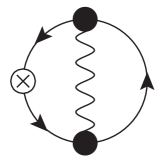
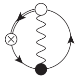
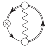
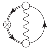
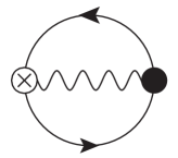
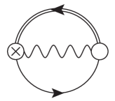
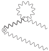
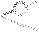
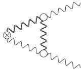
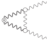
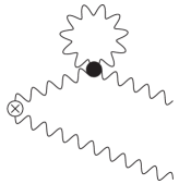
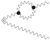
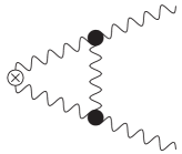
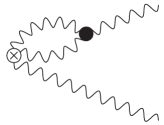
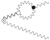
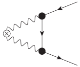
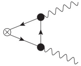
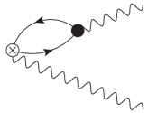
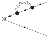
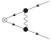
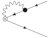
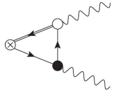
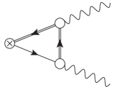
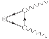
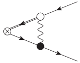
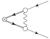
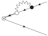
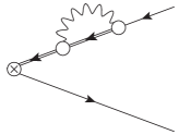
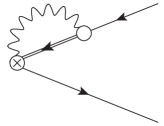
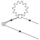
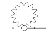
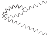
We now explain a diagrammatic representation of the perturbative expansion of flowed fields (the flow Feynman diagram). For quantum propagators (3.17) and (3.18), we use the standard convention that the free propagator of the gauge boson is denoted by a wavy line and the free propagator of the fermion is denoted by an arrowed straight line. We stick to these conventions because these are quite natural in a system containing fermions. In Refs. Suzuki:2013gza and Luscher:2011bx , on the other hand, the arrowed straight line was adopted to represent the gauge boson heat kernel (3.6). Since we already used this in this paper for the fermion propagator, we instead use “doubled lines” to represent heat kernels (3.6) and (3.14). For instance, Figs. 35 are one-loop flow Feynman diagrams which contribute to the two-point function of the flowed fermion field. In these figures, the doubled straight line represents the fermion heat kernel (3.14); the arrow denotes the flow of the fermion number, not the direction of the flow time. Similarly, in Fig. 16, the doubled wavy line is the gauge boson heat kernel (3.6). In the present representation, we thus lose the information of the direction of the flow time, which is represented by an arrow in Refs. Suzuki:2013gza and Luscher:2011bx . This information, however, can readily be traced back.

Another element of the flow Feynman diagram is the vertex. The vertices that come from the original action (2.1) are denoted by filled circles, while vertices that come through the flow equations, Eqs. (3.7), (3.15), and (3.16), are denoted by open circles as in Figs. 35; these conventions for the vertex are identical to those of Refs. Suzuki:2013gza and Luscher:2011bx .

3.2 Ringed fermion fields

A salient feature of the flowed fields is the UV finiteness: Any correlation functions of the flowed gauge field Bμ(t,x)subscript𝐵𝜇𝑡𝑥B_{\mu}(t,x) with strictly positive t𝑡t are, when expressed in terms of renormalized parameters, UV finite without the multiplicative (wave function) renormalization Luscher:2011bx . Moreover, this finiteness persists even for the equal-point limit. Thus, any correlation functions of any local products of Bμ(t,x)subscript𝐵𝜇𝑡𝑥B_{\mu}(t,x) (with t>0𝑡0t>0) are UV finite without further renormalization other than the parameter renormalization. In other words, although those local products are given by a certain combination of the bare gauge field Aμ(x)subscript𝐴𝜇𝑥A_{\mu}(x) through the flow equation, they are renormalized finite quantities. A basic reason for this UV finiteness is that the propagator of the flowed gauge field (3.17) contains the Gaussian dumping factor etp2similar-toabsentsuperscripte𝑡superscript𝑝2\sim\mathrm{e}^{-tp^{2}} which effectively provides a UV cutoff for t>0𝑡0t>0. To prove the above finiteness, however, one has to also utilize a Becchi–Rouet–Stora (BRS) symmetry underlying the present system that is inhomogeneous with respect to the gauge potential Luscher:2011bx .

Regrettably, the above finiteness in the first sense does not hold for the flowed fermion field. It requires the wave function renormalization. Although its propagator (3.18) also possesses the dumping factor etp2similar-toabsentsuperscripte𝑡superscript𝑝2\sim\mathrm{e}^{-tp^{2}}, the BRS transformation is homogeneous on the fermion field (and on general matter fields) and the finiteness proof in Ref. Luscher:2011bx does not apply. In fact, computation of the one-loop diagrams in Figs. 35 (and diagrams with opposite arrows) shows that the wave function renormalization

χR(t,x)=Zχ1/2χ(t,x),χ¯R(t,x)=Zχ1/2χ¯(t,x),Zχ=1+g2(4π)2C2(R)31ϵ+O(g4)formulae-sequencesubscript𝜒𝑅𝑡𝑥superscriptsubscript𝑍𝜒12𝜒𝑡𝑥formulae-sequencesubscript¯𝜒𝑅𝑡𝑥superscriptsubscript𝑍𝜒12¯𝜒𝑡𝑥subscript𝑍𝜒1superscript𝑔2superscript4𝜋2subscript𝐶2𝑅31italic-ϵ𝑂superscript𝑔4\chi_{R}(t,x)=Z_{\chi}^{1/2}\chi(t,x),\qquad\bar{\chi}_{R}(t,x)=Z_{\chi}^{1/2}\bar{\chi}(t,x),\qquad Z_{\chi}=1+\frac{g^{2}}{(4\pi)^{2}}C_{2}(R)3\frac{1}{\epsilon}+O(g^{4}) (3.19)

makes correlation functions UV finite Luscher:2013cpa . Finiteness in the above second sense still holds: Any correlation functions of any local products of χR(t,x)subscript𝜒𝑅𝑡𝑥\chi_{R}(t,x) and χ¯R(t,x)subscript¯𝜒𝑅𝑡𝑥\bar{\chi}_{R}(t,x) remain UV finite Luscher:2013cpa .
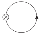
Refer to caption
Figure 1: C01
Refer to caption
Figure 2: C02
Refer to caption
Figure 3: C03
Refer to caption
Figure 4: C04
Refer to caption
Figure 5: C05

Although the finiteness in the second sense is quite useful for our purpose, we still need to incorporate the renormalization factor Zχsubscript𝑍𝜒Z_{\chi} in Eq. (3.19). This introduces a complication to our problem, because we have to find a matching factor between Zχsubscript𝑍𝜒Z_{\chi} in the dimensional regularization and that in the lattice regularization.

One possible way to avoid this complication is to normalize the fermion fields by the vacuum expectation value of the fermion kinetic operator:101010In the kinetic operator, the summation over Nfsubscript𝑁fN_{\mathrm{f}} fermion flavors is understood. In the first version of the present paper, we used the scalar condensation to normalize the fermion fields. This choice causes another complication associated with the massless fermion and the use of the kinetic operator seems much more appropriate.

χ̊(t,x)̊𝜒𝑡𝑥\displaystyle\mathring{\chi}(t,x) =2dim(R)Nf(4π)2t2χ¯(t,x)/Dχ(t,x)χ(t,x),absent2dimension𝑅subscript𝑁fsuperscript4𝜋2superscript𝑡2delimited-⟨⟩¯𝜒𝑡𝑥/𝐷𝜒𝑡𝑥𝜒𝑡𝑥\displaystyle=\sqrt{\frac{-2\dim(R)N_{\mathrm{f}}}{(4\pi)^{2}t^{2}\left\langle\bar{\chi}(t,x)\overleftrightarrow{{\ooalign{\hfil/\hfil\crcr$D$}}}\chi(t,x)\right\rangle}}\,\chi(t,x), (3.22)
χ¯̊(t,x)̊¯𝜒𝑡𝑥\displaystyle\mathring{\bar{\chi}}(t,x) =2dim(R)Nf(4π)2t2χ¯(t,x)/Dχ(t,x)χ¯(t,x),absent2dimension𝑅subscript𝑁fsuperscript4𝜋2superscript𝑡2delimited-⟨⟩¯𝜒𝑡𝑥/𝐷𝜒𝑡𝑥¯𝜒𝑡𝑥\displaystyle=\sqrt{\frac{-2\dim(R)N_{\mathrm{f}}}{(4\pi)^{2}t^{2}\left\langle\bar{\chi}(t,x)\overleftrightarrow{{\ooalign{\hfil/\hfil\crcr$D$}}}\chi(t,x)\right\rangle}}\,\bar{\chi}(t,x), (3.25)

where

DμDμDμ,subscript𝐷𝜇subscript𝐷𝜇subscript𝐷𝜇\overleftrightarrow{D}_{\mu}\equiv D_{\mu}-\overleftarrow{D}_{\mu}, (3.26)

so that the multiplicative renormalization factor Zχsubscript𝑍𝜒Z_{\chi} is cancelled out in the new ringed variables. Note that the mass dimension of χ̊(t,x)̊𝜒𝑡𝑥\mathring{\chi}(t,x) and χ¯̊(t,x)̊¯𝜒𝑡𝑥\mathring{\bar{\chi}}(t,x) is 3/2323/2 for any D𝐷D, while that of χ(t,x)𝜒𝑡𝑥\chi(t,x) and χ¯(t,x)¯𝜒𝑡𝑥\bar{\chi}(t,x) is (D1)/2𝐷12(D-1)/2.

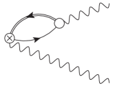
The vacuum expectation value of the kinetic operator in the lowest (one-loop) order approximation is given by diagram D01 in Fig. 6. For D=42ϵ𝐷42italic-ϵD=4-2\epsilon dimensions, we have

χ¯(t,x)/Dχ(t,x)=2dim(R)Nf(4π)2t2(8πt)ϵ[1+O(m02t)].delimited-⟨⟩¯𝜒𝑡𝑥/𝐷𝜒𝑡𝑥2dimension𝑅subscript𝑁fsuperscript4𝜋2superscript𝑡2superscript8𝜋𝑡italic-ϵdelimited-[]1𝑂superscriptsubscript𝑚02𝑡\left\langle\bar{\chi}(t,x)\overleftrightarrow{{\ooalign{\hfil/\hfil\crcr$D$}}}\chi(t,x)\right\rangle=\frac{-2\dim(R)N_{\mathrm{f}}}{(4\pi)^{2}t^{2}}(8\pi t)^{\epsilon}\left[1+O(m_{0}^{2}t)\right]. (3.27)

Note that the mass scale, which is required for the vacuum expectation value, is supplied by the flow time t𝑡t in the present setup. Having obtained this expression, the constant factors in Eqs. (3.22) and (3.25) have been chosen so that the difference between the ringed and the original variables becomes O(g02)𝑂superscriptsubscript𝑔02O(g_{0}^{2}) for sufficiently small flow time (m02t1much-less-thansuperscriptsubscript𝑚02𝑡1m_{0}^{2}t\ll 1).

Refer to caption
Figure 6: D01
Refer to caption
Figure 7: D02
Refer to caption
Figure 8: D03
Refer to caption
Figure 9: D04
Refer to caption
Figure 10: D05
Refer to caption
Figure 11: D06
Refer to caption
Figure 12: D07
Refer to caption
Figure 13: D08
Table 1: Contribution of each diagram to Eq. (3.31) in units of 2dim(R)Nf(4π)2t2g02(4π)2C2(R)2dimension𝑅subscript𝑁fsuperscript4𝜋2superscript𝑡2superscriptsubscript𝑔02superscript4𝜋2subscript𝐶2𝑅\frac{-2\dim(R)N_{\mathrm{f}}}{(4\pi)^{2}t^{2}}\frac{g_{0}^{2}}{(4\pi)^{2}}C_{2}(R).
      diagram
      D02       1ϵ2ln(8πt)+O(m02t)1italic-ϵ28𝜋𝑡𝑂superscriptsubscript𝑚02𝑡-\dfrac{1}{\epsilon}-2\ln(8\pi t)+O(m_{0}^{2}t)
      D03       21ϵ+4ln(8πt)+2+4ln22ln3+O(m02t)21italic-ϵ48𝜋𝑡24223𝑂superscriptsubscript𝑚02𝑡2\dfrac{1}{\epsilon}+4\ln(8\pi t)+2+4\ln 2-2\ln 3+O(m_{0}^{2}t)
      D04       20ln2+16ln3+O(m02t)202163𝑂superscriptsubscript𝑚02𝑡-20\ln 2+16\ln 3+O(m_{0}^{2}t)
      D05       12ln25ln3+O(m02t)12253𝑂superscriptsubscript𝑚02𝑡12\ln 2-5\ln 3+O(m_{0}^{2}t)
      D06       41ϵ8ln(8πt)2+O(m02t)41italic-ϵ88𝜋𝑡2𝑂superscriptsubscript𝑚02𝑡-4\dfrac{1}{\epsilon}-8\ln(8\pi t)-2+O(m_{0}^{2}t)
      D07       8ln24ln3+O(m02t)8243𝑂superscriptsubscript𝑚02𝑡8\ln 2-4\ln 3+O(m_{0}^{2}t)
      D08       2ln3+O(m02t)23𝑂superscriptsubscript𝑚02𝑡-2\ln 3+O(m_{0}^{2}t)

The next-to-leading-order (i.e., two-loop) expression for the expectation value (3.27) is given by the flow Feynman diagrams in Figs. 913 (and diagrams with arrows with the opposite direction). The computation of these diagrams is somewhat complicated but can be completed in a similar manner to the calculation in Appendix B of Ref. Luscher:2010iy [with the integration formulas in our Appendix B, Eqs. (B.1) and (B.2)]. The contribution of each diagram is tabulated in Table 1. In total, we have

χ¯(t,x)/Dχ(t,x)delimited-⟨⟩¯𝜒𝑡𝑥/𝐷𝜒𝑡𝑥\displaystyle\left\langle\bar{\chi}(t,x)\overleftrightarrow{{\ooalign{\hfil/\hfil\crcr$D$}}}\chi(t,x)\right\rangle (3.30)
=2dim(R)Nf(4π)2t2{(8πt)ϵ+g02(4π)2C2(R)[31ϵ6ln(8πt)+ln(432)]+O(m02t)+O(g04)}.absent2dimension𝑅subscript𝑁fsuperscript4𝜋2superscript𝑡2superscript8𝜋𝑡italic-ϵsuperscriptsubscript𝑔02superscript4𝜋2subscript𝐶2𝑅delimited-[]31italic-ϵ68𝜋𝑡432𝑂superscriptsubscript𝑚02𝑡𝑂superscriptsubscript𝑔04\displaystyle=\frac{-2\dim(R)N_{\mathrm{f}}}{(4\pi)^{2}t^{2}}\left\{(8\pi t)^{\epsilon}+\frac{g_{0}^{2}}{(4\pi)^{2}}C_{2}(R)\left[-3\frac{1}{\epsilon}-6\ln(8\pi t)+\ln(432)\right]+O(m_{0}^{2}t)+O(g_{0}^{4})\right\}. (3.31)

Using Eq. (A.1) for the normalization factor in Eqs. (3.22) and (3.25), we have

2dim(R)Nf(4π)2t2χ¯(t,x)/Dχ(t,x)=Z(ϵ){1+g2(4π)2C2(R)[31ϵΦ(t)]+O(m2t)+O(g4)},2dimension𝑅subscript𝑁fsuperscript4𝜋2superscript𝑡2delimited-⟨⟩¯𝜒𝑡𝑥/𝐷𝜒𝑡𝑥𝑍italic-ϵ1superscript𝑔2superscript4𝜋2subscript𝐶2𝑅delimited-[]31italic-ϵΦ𝑡𝑂superscript𝑚2𝑡𝑂superscript𝑔4\frac{-2\dim(R)N_{\mathrm{f}}}{(4\pi)^{2}t^{2}\left\langle\bar{\chi}(t,x)\overleftrightarrow{{\ooalign{\hfil/\hfil\crcr$D$}}}\chi(t,x)\right\rangle}=Z(\epsilon)\left\{1+\frac{g^{2}}{(4\pi)^{2}}C_{2}(R)\left[3\frac{1}{\epsilon}-\Phi(t)\right]+O(m^{2}t)+O(g^{4})\right\}, (3.32)

where

Z(ϵ)1(8πt)ϵ,𝑍italic-ϵ1superscript8𝜋𝑡italic-ϵZ(\epsilon)\equiv\frac{1}{(8\pi t)^{\epsilon}}, (3.33)

and

Φ(t)3ln(8πμ2t)+ln(432).Φ𝑡38𝜋superscript𝜇2𝑡432\Phi(t)\equiv-3\ln(8\pi\mu^{2}t)+\ln(432). (3.34)

4 Energy–momentum tensor constructed from the flowed fields

4.1 Small flow-time expansion and the renormalization group argument

To express the energy–momentum tensor in Eqs. (2.9) and (2.12) in terms of the flowed fields, we consider following second-rank symmetric tensors (which are even under the CP transformation) constructed from the flowed fields:

𝒪~1μν(t,x)subscript~𝒪1𝜇𝜈𝑡𝑥\displaystyle\tilde{\mathcal{O}}_{1\mu\nu}(t,x) Gμρa(t,x)Gνρa(t,x),absentsuperscriptsubscript𝐺𝜇𝜌𝑎𝑡𝑥superscriptsubscript𝐺𝜈𝜌𝑎𝑡𝑥\displaystyle\equiv G_{\mu\rho}^{a}(t,x)G_{\nu\rho}^{a}(t,x), (4.1)
𝒪~2μν(t,x)subscript~𝒪2𝜇𝜈𝑡𝑥\displaystyle\tilde{\mathcal{O}}_{2\mu\nu}(t,x) δμνGρσa(t,x)Gρσa(t,x),absentsubscript𝛿𝜇𝜈superscriptsubscript𝐺𝜌𝜎𝑎𝑡𝑥superscriptsubscript𝐺𝜌𝜎𝑎𝑡𝑥\displaystyle\equiv\delta_{\mu\nu}G_{\rho\sigma}^{a}(t,x)G_{\rho\sigma}^{a}(t,x), (4.2)
𝒪~3μν(t,x)subscript~𝒪3𝜇𝜈𝑡𝑥\displaystyle\tilde{\mathcal{O}}_{3\mu\nu}(t,x) χ¯̊(t,x)(γμDν+γνDμ)χ̊(t,x),absent̊¯𝜒𝑡𝑥subscript𝛾𝜇subscript𝐷𝜈subscript𝛾𝜈subscript𝐷𝜇̊𝜒𝑡𝑥\displaystyle\equiv\mathring{\bar{\chi}}(t,x)\left(\gamma_{\mu}\overleftrightarrow{D}_{\nu}+\gamma_{\nu}\overleftrightarrow{D}_{\mu}\right)\mathring{\chi}(t,x), (4.3)
𝒪~4μν(t,x)subscript~𝒪4𝜇𝜈𝑡𝑥\displaystyle\tilde{\mathcal{O}}_{4\mu\nu}(t,x) δμνχ¯̊(t,x)/Dχ̊(t,x),absentsubscript𝛿𝜇𝜈̊¯𝜒𝑡𝑥/𝐷̊𝜒𝑡𝑥\displaystyle\equiv\delta_{\mu\nu}\mathring{\bar{\chi}}(t,x)\overleftrightarrow{{\ooalign{\hfil/\hfil\crcr$D$}}}\mathring{\chi}(t,x), (4.6)
𝒪~5μν(t,x)subscript~𝒪5𝜇𝜈𝑡𝑥\displaystyle\tilde{\mathcal{O}}_{5\mu\nu}(t,x) δμνmχ¯̊(t,x)χ̊(t,x).absentsubscript𝛿𝜇𝜈𝑚̊¯𝜒𝑡𝑥̊𝜒𝑡𝑥\displaystyle\equiv\delta_{\mu\nu}m\mathring{\bar{\chi}}(t,x)\mathring{\chi}(t,x). (4.7)

Note that all the above operators 𝒪~iμν(t,x)subscript~𝒪𝑖𝜇𝜈𝑡𝑥\tilde{\mathcal{O}}_{i\mu\nu}(t,x) are of dimension 444 for any D𝐷D.

We also introduce corresponding bare operators in the D𝐷D-dimensional x𝑥x-space:

𝒪1μν(x)subscript𝒪1𝜇𝜈𝑥\displaystyle\mathcal{O}_{1\mu\nu}(x) Fμρa(x)Fνρa(x),absentsuperscriptsubscript𝐹𝜇𝜌𝑎𝑥superscriptsubscript𝐹𝜈𝜌𝑎𝑥\displaystyle\equiv F_{\mu\rho}^{a}(x)F_{\nu\rho}^{a}(x), (4.8)
𝒪2μν(x)subscript𝒪2𝜇𝜈𝑥\displaystyle\mathcal{O}_{2\mu\nu}(x) δμνFρσa(x)Fρσa(x),absentsubscript𝛿𝜇𝜈superscriptsubscript𝐹𝜌𝜎𝑎𝑥superscriptsubscript𝐹𝜌𝜎𝑎𝑥\displaystyle\equiv\delta_{\mu\nu}F_{\rho\sigma}^{a}(x)F_{\rho\sigma}^{a}(x), (4.9)
𝒪3μν(x)subscript𝒪3𝜇𝜈𝑥\displaystyle\mathcal{O}_{3\mu\nu}(x) ψ¯(x)(γμDν+γνDμ)ψ(x),absent¯𝜓𝑥subscript𝛾𝜇subscript𝐷𝜈subscript𝛾𝜈subscript𝐷𝜇𝜓𝑥\displaystyle\equiv\bar{\psi}(x)\left(\gamma_{\mu}\overleftrightarrow{D}_{\nu}+\gamma_{\nu}\overleftrightarrow{D}_{\mu}\right)\psi(x), (4.10)
𝒪4μν(x)subscript𝒪4𝜇𝜈𝑥\displaystyle\mathcal{O}_{4\mu\nu}(x) δμνψ¯(x)/Dψ(x),absentsubscript𝛿𝜇𝜈¯𝜓𝑥/𝐷𝜓𝑥\displaystyle\equiv\delta_{\mu\nu}\bar{\psi}(x)\overleftrightarrow{{\ooalign{\hfil/\hfil\crcr$D$}}}\psi(x), (4.13)
𝒪5μν(x)subscript𝒪5𝜇𝜈𝑥\displaystyle\mathcal{O}_{5\mu\nu}(x) δμνm0ψ¯(x)ψ(x).absentsubscript𝛿𝜇𝜈subscript𝑚0¯𝜓𝑥𝜓𝑥\displaystyle\equiv\delta_{\mu\nu}m_{0}\bar{\psi}(x)\psi(x). (4.14)

The mass dimension of 𝒪1μν(x)subscript𝒪1𝜇𝜈𝑥\mathcal{O}_{1\mu\nu}(x) and 𝒪2μν(x)subscript𝒪2𝜇𝜈𝑥\mathcal{O}_{2\mu\nu}(x) is 444, while that of 𝒪3μν(x)subscript𝒪3𝜇𝜈𝑥\mathcal{O}_{3\mu\nu}(x), 𝒪4μν(x)subscript𝒪4𝜇𝜈𝑥\mathcal{O}_{4\mu\nu}(x), and 𝒪5μν(x)subscript𝒪5𝜇𝜈𝑥\mathcal{O}_{5\mu\nu}(x) is D𝐷D.

We now consider the situation in which the flow time t𝑡t in Eqs. (4.1)–(4.7) is very small. Since a flowed field at position x𝑥x with a flow time t𝑡t is a combination of un-flowed fields in the vicinity of x𝑥x of radius 8tsimilar-toabsent8𝑡\sim\sqrt{8t},111111This follows from the fact that the flow equations are basically the diffusion equation. the operators (4.1)–(4.7) can be regarded as local operators in x𝑥x-space in the t0𝑡0t\to 0 limit. Since the bare operators in Eqs. (4.8)–(4.14) span a complete set of symmetric second-rank gauge-invariant local operators of dimension 444 (for D4𝐷4D\to 4) which are even under CP, we have the following (asymptotic) expansion for small t𝑡t:

𝒪~iμν(t,x)=𝒪~iμν(t,x)+ζij(t)[𝒪jμν(x)𝒪jμν(x)]+O(t),subscript~𝒪𝑖𝜇𝜈𝑡𝑥delimited-⟨⟩subscript~𝒪𝑖𝜇𝜈𝑡𝑥subscript𝜁𝑖𝑗𝑡delimited-[]subscript𝒪𝑗𝜇𝜈𝑥delimited-⟨⟩subscript𝒪𝑗𝜇𝜈𝑥𝑂𝑡\tilde{\mathcal{O}}_{i\mu\nu}(t,x)=\left\langle\tilde{\mathcal{O}}_{i\mu\nu}(t,x)\right\rangle+\zeta_{ij}(t)\left[\mathcal{O}_{j\mu\nu}(x)-\left\langle\mathcal{O}_{j\mu\nu}(x)\right\rangle\right]+O(t), (4.15)

where the abbreviated terms are contributions of operators of mass dimension 666 (for D4𝐷4D\to 4) or higher.

In writing down the small flow-time expansion (4.15), we have assumed that there is no other D𝐷D-dimensional composite operator at the point x𝑥x. That the expansion (4.15) cannot necessarily hold when there is another operator at the point x𝑥x [say, 𝒫(x)𝒫𝑥\mathcal{P}(x)] can be seen by noting that the product of the left-hand side of Eq. (4.15) with 𝒫(x)𝒫𝑥\mathcal{P}(x) does not possess any divergence for t>0𝑡0t>0, while each term in the right-hand side can have an equal-point singularity with 𝒫(x)𝒫𝑥\mathcal{P}(x) because the operators in the right-hand side of Eq. (4.15) are D𝐷D-dimensional (i.e., non-flowed) composite operators. This is a contradiction if Eq. (4.15) holds. This implies that the formula we will derive for the energy–momentum tensor below holds only when the energy–momentum tensor has no overlap with other operators.121212This important point was not fully recognized in Ref. Suzuki:2013gza . In particular, we cannot say anything about whether the Ward–Takahashi relation (2.11) is reproduced with our construction. Still, our construction is expected to have a correct normalization because it is determined from matching the energy–momentum tensor in the dimensional regularization which fulfills Eq. (2.11). Our lattice energy–momentum tensor is thus useful to compute correlation functions in which the energy–momentum tensor is separated from other operators. This is the case for correlation functions relevant to the viscosities Nakamura:2004sy ; Meyer:2007ic ; Meyer:2007dy , for example.

The expansion (4.15) may be inverted as

𝒪iμν(x)𝒪iμν(x)=(ζ1)ij(t)[𝒪~jμν(t,x)𝒪~jμν(t,x)]+O(t),subscript𝒪𝑖𝜇𝜈𝑥delimited-⟨⟩subscript𝒪𝑖𝜇𝜈𝑥subscriptsuperscript𝜁1𝑖𝑗𝑡delimited-[]subscript~𝒪𝑗𝜇𝜈𝑡𝑥delimited-⟨⟩subscript~𝒪𝑗𝜇𝜈𝑡𝑥𝑂𝑡\mathcal{O}_{i\mu\nu}(x)-\left\langle\mathcal{O}_{i\mu\nu}(x)\right\rangle=\left(\zeta^{-1}\right)_{ij}(t)\left[\tilde{\mathcal{O}}_{j\mu\nu}(t,x)-\left\langle\tilde{\mathcal{O}}_{j\mu\nu}(t,x)\right\rangle\right]+O(t), (4.16)

where ζ1superscript𝜁1\zeta^{-1} denotes the inverse matrix of ζ𝜁\zeta. Then, by substituting this relation into the energy–momentum tensor (2.9) and (2.12) in terms of the bare operators,

{Tμν}R(x)subscriptsubscript𝑇𝜇𝜈𝑅𝑥\displaystyle\left\{T_{\mu\nu}\right\}_{R}(x) =1g02{𝒪1μν(x)𝒪1μν(x)14[𝒪2μν(x)𝒪2μν(x)]}absent1superscriptsubscript𝑔02subscript𝒪1𝜇𝜈𝑥delimited-⟨⟩subscript𝒪1𝜇𝜈𝑥14delimited-[]subscript𝒪2𝜇𝜈𝑥delimited-⟨⟩subscript𝒪2𝜇𝜈𝑥\displaystyle=\frac{1}{g_{0}^{2}}\left\{\mathcal{O}_{1\mu\nu}(x)-\left\langle\mathcal{O}_{1\mu\nu}(x)\right\rangle-\frac{1}{4}\left[\mathcal{O}_{2\mu\nu}(x)-\left\langle\mathcal{O}_{2\mu\nu}(x)\right\rangle\right]\right\}
+14[𝒪3μν(x)𝒪3μν(x)]12[𝒪4μν(x)𝒪4μν(x)]14delimited-[]subscript𝒪3𝜇𝜈𝑥delimited-⟨⟩subscript𝒪3𝜇𝜈𝑥12delimited-[]subscript𝒪4𝜇𝜈𝑥delimited-⟨⟩subscript𝒪4𝜇𝜈𝑥\displaystyle\qquad{}+\frac{1}{4}\left[\mathcal{O}_{3\mu\nu}(x)-\left\langle\mathcal{O}_{3\mu\nu}(x)\right\rangle\right]-\frac{1}{2}\left[\mathcal{O}_{4\mu\nu}(x)-\left\langle\mathcal{O}_{4\mu\nu}(x)\right\rangle\right]
[𝒪5μν(x)𝒪5μν(x)],delimited-[]subscript𝒪5𝜇𝜈𝑥delimited-⟨⟩subscript𝒪5𝜇𝜈𝑥\displaystyle\qquad\qquad{}-\left[\mathcal{O}_{5\mu\nu}(x)-\left\langle\mathcal{O}_{5\mu\nu}(x)\right\rangle\right], (4.17)

we have the expression (for D=4𝐷4D=4)

{Tμν}R(x)subscriptsubscript𝑇𝜇𝜈𝑅𝑥\displaystyle\left\{T_{\mu\nu}\right\}_{R}(x) =c1(t)[𝒪~1μν(t,x)14𝒪~2μν(t,x)]absentsubscript𝑐1𝑡delimited-[]subscript~𝒪1𝜇𝜈𝑡𝑥14subscript~𝒪2𝜇𝜈𝑡𝑥\displaystyle=c_{1}(t)\left[\tilde{\mathcal{O}}_{1\mu\nu}(t,x)-\frac{1}{4}\tilde{\mathcal{O}}_{2\mu\nu}(t,x)\right]
+c2(t)[𝒪~2μν(t,x)𝒪~2μν(t,x)]subscript𝑐2𝑡delimited-[]subscript~𝒪2𝜇𝜈𝑡𝑥delimited-⟨⟩subscript~𝒪2𝜇𝜈𝑡𝑥\displaystyle\qquad{}+c_{2}(t)\left[\tilde{\mathcal{O}}_{2\mu\nu}(t,x)-\left\langle\tilde{\mathcal{O}}_{2\mu\nu}(t,x)\right\rangle\right]
+c3(t)[𝒪~3μν(t,x)2𝒪~4μν(t,x)𝒪~3μν(t,x)2𝒪~4μν(t,x)]subscript𝑐3𝑡delimited-[]subscript~𝒪3𝜇𝜈𝑡𝑥2subscript~𝒪4𝜇𝜈𝑡𝑥delimited-⟨⟩subscript~𝒪3𝜇𝜈𝑡𝑥2subscript~𝒪4𝜇𝜈𝑡𝑥\displaystyle\qquad\qquad{}+c_{3}(t)\left[\tilde{\mathcal{O}}_{3\mu\nu}(t,x)-2\tilde{\mathcal{O}}_{4\mu\nu}(t,x)-\left\langle\tilde{\mathcal{O}}_{3\mu\nu}(t,x)-2\tilde{\mathcal{O}}_{4\mu\nu}(t,x)\right\rangle\right]
+c4(t)[𝒪~4μν(t,x)𝒪~4μν(t,x)]subscript𝑐4𝑡delimited-[]subscript~𝒪4𝜇𝜈𝑡𝑥delimited-⟨⟩subscript~𝒪4𝜇𝜈𝑡𝑥\displaystyle\qquad\qquad\qquad{}+c_{4}(t)\left[\tilde{\mathcal{O}}_{4\mu\nu}(t,x)-\left\langle\tilde{\mathcal{O}}_{4\mu\nu}(t,x)\right\rangle\right]
+c5(t)[𝒪~5μν(t,x)𝒪~5μν(t,x)]+O(t),subscript𝑐5𝑡delimited-[]subscript~𝒪5𝜇𝜈𝑡𝑥delimited-⟨⟩subscript~𝒪5𝜇𝜈𝑡𝑥𝑂𝑡\displaystyle\qquad\qquad\qquad\qquad{}+c_{5}(t)\left[\tilde{\mathcal{O}}_{5\mu\nu}(t,x)-\left\langle\tilde{\mathcal{O}}_{5\mu\nu}(t,x)\right\rangle\right]+O(t), (4.18)

where

c1(t)=c~1(t),c2(t)=c~2(t)+14c1(t),formulae-sequencesubscript𝑐1𝑡subscript~𝑐1𝑡subscript𝑐2𝑡subscript~𝑐2𝑡14subscript𝑐1𝑡\displaystyle c_{1}(t)=\tilde{c}_{1}(t),\qquad c_{2}(t)=\tilde{c}_{2}(t)+\frac{1}{4}c_{1}(t),
c3(t)=c~3(t),c4(t)=c~4(t)+2c3(t),c5(t)=c~5(t),formulae-sequencesubscript𝑐3𝑡subscript~𝑐3𝑡formulae-sequencesubscript𝑐4𝑡subscript~𝑐4𝑡2subscript𝑐3𝑡subscript𝑐5𝑡subscript~𝑐5𝑡\displaystyle c_{3}(t)=\tilde{c}_{3}(t),\qquad c_{4}(t)=\tilde{c}_{4}(t)+2c_{3}(t),\qquad c_{5}(t)=\tilde{c}_{5}(t), (4.19)

and

c~i(t)1g02{(ζ1)1i(t)14(ζ1)2i(t)}+14(ζ1)3i(t)12(ζ1)4i(t)(ζ1)5i(t).subscript~𝑐𝑖𝑡1superscriptsubscript𝑔02subscriptsuperscript𝜁11𝑖𝑡14subscriptsuperscript𝜁12𝑖𝑡14subscriptsuperscript𝜁13𝑖𝑡12subscriptsuperscript𝜁14𝑖𝑡subscriptsuperscript𝜁15𝑖𝑡\tilde{c}_{i}(t)\equiv\frac{1}{g_{0}^{2}}\left\{\left(\zeta^{-1}\right)_{1i}(t)-\frac{1}{4}\left(\zeta^{-1}\right)_{2i}(t)\right\}+\frac{1}{4}\left(\zeta^{-1}\right)_{3i}(t)-\frac{1}{2}\left(\zeta^{-1}\right)_{4i}(t)-\left(\zeta^{-1}\right)_{5i}(t). (4.20)

In Eq. (4.18), we have used the fact that the finite operator 𝒪~1μν(t,x)(1/4)𝒪~2μν(t,x)subscript~𝒪1𝜇𝜈𝑡𝑥14subscript~𝒪2𝜇𝜈𝑡𝑥\tilde{\mathcal{O}}_{1\mu\nu}(t,x)-(1/4)\tilde{\mathcal{O}}_{2\mu\nu}(t,x) is traceless in D=4𝐷4D=4 and thus has no vacuum expectation value. Equation (4.18) shows that if one knows the t0𝑡0t\to 0 behavior of the coefficients ci(t)subscript𝑐𝑖𝑡c_{i}(t), the energy–momentum tensor can be obtained as the t0𝑡0t\to 0 limit of the combination in the right-hand side. As already noted, since the composite operators (4.1)–(4.7) constructed from (ringed) flowed fields should be independent of the regularization adopted, one may use the lattice regularization to compute correlation functions of the quantity in the right-hand side of Eq. (4.18). This provides a possible method to compute correlation functions of the correctly normalized conserved energy–momentum tensor with the lattice regularization.

Thus, we are interested in the t0𝑡0t\to 0 behavior of the coefficients ci(t)subscript𝑐𝑖𝑡c_{i}(t) in Eq. (4.18). Quite interestingly, one can argue that the coefficients ci(t)subscript𝑐𝑖𝑡c_{i}(t) can be evaluated by the perturbation theory for t0𝑡0t\to 0 thanks to the asymptotic freedom. To see this, we apply

(μμ)0subscript𝜇𝜇0\left(\mu\frac{\partial}{\partial\mu}\right)_{0} (4.21)

on both sides of Eq. (4.18), where μ𝜇\mu is the renormalization scale and the subscript 00 implies that the derivative is taken while all bare quantities are kept fixed. Since the energy–momentum tensor is not multiplicatively renormalized, (μ/μ)0(left-hand side of Eq. (4.18))=0subscript𝜇𝜇0left-hand side of Eq. (4.18)0(\mu\partial/\partial\mu)_{0}(\text{left-hand side of Eq.~{}\eqref{eq:(4.14)}})=0. On the right-hand side, since O~1,2,3,4μν(t,x)subscript~𝑂1234𝜇𝜈𝑡𝑥\tilde{O}_{1,2,3,4\mu\nu}(t,x) and (1/m)O~5μν(t,x)1𝑚subscript~𝑂5𝜇𝜈𝑡𝑥(1/m)\tilde{O}_{5\mu\nu}(t,x) are entirely given by bare quantities through the flow equations, we have

(μμ)0O~1,2,3,4μν(t,x)=(μμ)01mO~5μν(t,x)=0.subscript𝜇𝜇0subscript~𝑂1234𝜇𝜈𝑡𝑥subscript𝜇𝜇01𝑚subscript~𝑂5𝜇𝜈𝑡𝑥0\left(\mu\frac{\partial}{\partial\mu}\right)_{0}\tilde{O}_{1,2,3,4\mu\nu}(t,x)=\left(\mu\frac{\partial}{\partial\mu}\right)_{0}\frac{1}{m}\tilde{O}_{5\mu\nu}(t,x)=0. (4.22)

These observations imply

(μμ)0c1,2,3,4(t)=(μμ)0mc5(t)=0.subscript𝜇𝜇0subscript𝑐1234𝑡subscript𝜇𝜇0𝑚subscript𝑐5𝑡0\left(\mu\frac{\partial}{\partial\mu}\right)_{0}c_{1,2,3,4}(t)=\left(\mu\frac{\partial}{\partial\mu}\right)_{0}mc_{5}(t)=0. (4.23)

Then the standard renormalization group argument says that c1,2,3,4(t)subscript𝑐1234𝑡c_{1,2,3,4}(t) and mc5(t)𝑚subscript𝑐5𝑡mc_{5}(t) are independent of the renormalization scale, if the renormalized parameters in these quantities are replaced by running parameters defined by

qdg¯(q)dq=β(g¯(q)),g¯(q=μ)=g,formulae-sequence𝑞d¯𝑔𝑞d𝑞𝛽¯𝑔𝑞¯𝑔𝑞𝜇𝑔\displaystyle q\frac{\mathrm{d}\bar{g}(q)}{\mathrm{d}q}=\beta(\bar{g}(q)),\qquad\bar{g}(q=\mu)=g, (4.24)
qdm¯(q)dq=γm(g¯(q))m¯(q),m¯(q=μ)=m,formulae-sequence𝑞d¯𝑚𝑞d𝑞subscript𝛾𝑚¯𝑔𝑞¯𝑚𝑞¯𝑚𝑞𝜇𝑚\displaystyle q\frac{\mathrm{d}\bar{m}(q)}{\mathrm{d}q}=-\gamma_{m}(\bar{g}(q))\bar{m}(q),\qquad\bar{m}(q=\mu)=m, (4.25)

where μ𝜇\mu is the original renormalization scale. Thus, since c1,2,3,4(t)subscript𝑐1234𝑡c_{1,2,3,4}(t) and mc5(t)𝑚subscript𝑐5𝑡mc_{5}(t) are independent of the renormalization scale, two possible choices, q=μ𝑞𝜇q=\mu and q=1/8t𝑞18𝑡q=1/\sqrt{8t}, should give an identical result. In this way, we infer that

c1,2,3,4(t)(g,m;μ)subscript𝑐1234𝑡𝑔𝑚𝜇\displaystyle c_{1,2,3,4}(t)(g,m;\mu) =c1,2,3,4(t)(g¯(1/8t),m¯(1/8t);1/8t),absentsubscript𝑐1234𝑡¯𝑔18𝑡¯𝑚18𝑡18𝑡\displaystyle=c_{1,2,3,4}(t)(\bar{g}(1/\sqrt{8t}),\bar{m}(1/\sqrt{8t});1/\sqrt{8t}), (4.26)
c5(t)(g,m;μ)subscript𝑐5𝑡𝑔𝑚𝜇\displaystyle c_{5}(t)(g,m;\mu) =m¯(1/8t)mc5(t)(g¯(1/8t),m¯(1/8t);1/8t),absent¯𝑚18𝑡𝑚subscript𝑐5𝑡¯𝑔18𝑡¯𝑚18𝑡18𝑡\displaystyle=\frac{\bar{m}(1/\sqrt{8t})}{m}c_{5}(t)(\bar{g}(1/\sqrt{8t}),\bar{m}(1/\sqrt{8t});1/\sqrt{8t}), (4.27)

where we have explicitly written the dependence of ci(t)subscript𝑐𝑖𝑡c_{i}(t) on renormalized parameters and on the renormalization scale. Finally, since the running gauge coupling g¯(1/8t)0¯𝑔18𝑡0\bar{g}(1/\sqrt{8t})\to 0 for t0𝑡0t\to 0 thanks to the asymptotic freedom, we expect that we can compute ci(t)subscript𝑐𝑖𝑡c_{i}(t) for t0𝑡0t\to 0 by using the perturbation theory. Although we are interested in low-energy physics for which the perturbation theory is ineffective, the coefficients ci(t)subscript𝑐𝑖𝑡c_{i}(t) in Eq. (4.18) for t0𝑡0t\to 0 can be evaluated by perturbation theory; this might be regarded as a sort of factorization.

4.2 ci(t)subscript𝑐𝑖𝑡c_{i}(t) to the one-loop order

We thus evaluate the above coefficients ci(t)subscript𝑐𝑖𝑡c_{i}(t) in Eq. (4.18) to the one-loop order approximation. For this, we compute the mixing coefficients ζij(t)subscript𝜁𝑖𝑗𝑡\zeta_{ij}(t) in Eq. (4.15) to the one-loop order. Then ci(t)subscript𝑐𝑖𝑡c_{i}(t) are obtained by Eqs. (4.19) and (4.20). The loop expansion of ζij(t)subscript𝜁𝑖𝑗𝑡\zeta_{ij}(t) would yield

ζij(t)=δij+ζij(1)(t)+ζij(2)(t)+,subscript𝜁𝑖𝑗𝑡subscript𝛿𝑖𝑗superscriptsubscript𝜁𝑖𝑗1𝑡superscriptsubscript𝜁𝑖𝑗2𝑡\zeta_{ij}(t)=\delta_{ij}+\zeta_{ij}^{(1)}(t)+\zeta_{ij}^{(2)}(t)+\dotsb, (4.28)

for j=1𝑗1j=1 and j=2𝑗2j=2, where the superscript denotes the loop order, and for j=3𝑗3j=3, 444, and 555, by taking the factor in Eq. (3.33) into account, we set

ζij(t)=Z(ϵ)[δij+ζij(1)(t)+ζij(2)(t)+].subscript𝜁𝑖𝑗𝑡𝑍italic-ϵdelimited-[]subscript𝛿𝑖𝑗superscriptsubscript𝜁𝑖𝑗1𝑡superscriptsubscript𝜁𝑖𝑗2𝑡\zeta_{ij}(t)=Z(\epsilon)\left[\delta_{ij}+\zeta_{ij}^{(1)}(t)+\zeta_{ij}^{(2)}(t)+\dotsb\right]. (4.29)

As Ref. Suzuki:2013gza , it is straightforward to compute ζij(1)(t)superscriptsubscript𝜁𝑖𝑗1𝑡\zeta_{ij}^{(1)}(t).131313The justification for the following computational prescription was not well explained in previous versions of the present paper: One may wonder why the one-loop matching coefficients ζij(1)(t)superscriptsubscript𝜁𝑖𝑗1𝑡\zeta_{ij}^{(1)}(t) can be read off from the correlation functions (4.30) and (4.33) alone, without computing corresponding correlation functions in which flowed composite operators 𝒪~iμν(t,x)subscript~𝒪𝑖𝜇𝜈𝑡𝑥\tilde{\mathcal{O}}_{i\mu\nu}(t,x) are replaced by bare ones 𝒪iμν(x)subscript𝒪𝑖𝜇𝜈𝑥\mathcal{O}_{i\mu\nu}(x). The justification is directly related to our way of treatment of infrared (IR) divergences and we supplement detailed explanation in Appendix D. We are quite grateful to a referee of the present paper for suggestions on this point. For example, to obtain ζij(1)(t)superscriptsubscript𝜁𝑖𝑗1𝑡\zeta_{ij}^{(1)}(t) with j=1𝑗1j=1 and 222, we consider the correlation function

𝒪~iμν(t,x)Aβb(y)Aγc(z).delimited-⟨⟩subscript~𝒪𝑖𝜇𝜈𝑡𝑥superscriptsubscript𝐴𝛽𝑏𝑦superscriptsubscript𝐴𝛾𝑐𝑧\left\langle\tilde{\mathcal{O}}_{i\mu\nu}(t,x)A_{\beta}^{b}(y)A_{\gamma}^{c}(z)\right\rangle. (4.30)

In the Feynman gauge which we use throughout the present paper, this has the structure

g02keik(xy)k2g02ei(xz)2δbcμν,βγ(k,).superscriptsubscript𝑔02subscript𝑘superscripte𝑖𝑘𝑥𝑦superscript𝑘2superscriptsubscript𝑔02subscriptsuperscripte𝑖𝑥𝑧superscript2superscript𝛿𝑏𝑐subscript𝜇𝜈𝛽𝛾𝑘g_{0}^{2}\int_{k}\frac{\mathrm{e}^{ik(x-y)}}{k^{2}}g_{0}^{2}\int_{\ell}\frac{\mathrm{e}^{i\ell(x-z)}}{\ell^{2}}\delta^{bc}\mathcal{M}_{\mu\nu,\beta\gamma}(k,\ell). (4.31)

After expanding μν,βγ(k,)subscript𝜇𝜈𝛽𝛾𝑘\mathcal{M}_{\mu\nu,\beta\gamma}(k,\ell) to O(k,)𝑂𝑘O(k,\ell), we can make use of the following correspondence to read off the operator mixing:

ikμiνδβγFμρa(x)Fνρa(x),ikiδμνδβγ14δμνFρσa(x)Fρσa(x).formulae-sequence𝑖subscript𝑘𝜇𝑖subscript𝜈subscript𝛿𝛽𝛾superscriptsubscript𝐹𝜇𝜌𝑎𝑥superscriptsubscript𝐹𝜈𝜌𝑎𝑥𝑖𝑘𝑖subscript𝛿𝜇𝜈subscript𝛿𝛽𝛾14subscript𝛿𝜇𝜈superscriptsubscript𝐹𝜌𝜎𝑎𝑥superscriptsubscript𝐹𝜌𝜎𝑎𝑥ik_{\mu}i\ell_{\nu}\delta_{\beta\gamma}\to F_{\mu\rho}^{a}(x)F_{\nu\rho}^{a}(x),\qquad ik\cdot i\ell\delta_{\mu\nu}\delta_{\beta\gamma}\to\frac{1}{4}\delta_{\mu\nu}F_{\rho\sigma}^{a}(x)F_{\rho\sigma}^{a}(x). (4.32)

In this way, we obtain ζij(1)(t)superscriptsubscript𝜁𝑖𝑗1𝑡\zeta_{ij}^{(1)}(t) with j=1𝑗1j=1 and 222.141414For the momentum integration, we use the integration formulas in Appendix B.

Similarly, to obtain ζij(1)(t)superscriptsubscript𝜁𝑖𝑗1𝑡\zeta_{ij}^{(1)}(t) with j=3𝑗3j=3, 444, and 555, we consider

𝒪~iμν(t,x)ψ(y)ψ¯(z),delimited-⟨⟩subscript~𝒪𝑖𝜇𝜈𝑡𝑥𝜓𝑦¯𝜓𝑧\left\langle\tilde{\mathcal{O}}_{i\mu\nu}(t,x)\psi(y)\bar{\psi}(z)\right\rangle, (4.33)

whose general structure reads

keik(yx)i/k+m0μν(k,)ei(xz)i/+m0.subscript𝑘superscripte𝑖𝑘𝑦𝑥𝑖/𝑘subscript𝑚0subscript𝜇𝜈𝑘subscriptsuperscripte𝑖𝑥𝑧𝑖/subscript𝑚0\int_{k}\frac{\mathrm{e}^{ik(y-x)}}{i{\ooalign{\hfil/\hfil\crcr$k$}}+m_{0}}\mathcal{M}_{\mu\nu}(k,\ell)\int_{\ell}\frac{\mathrm{e}^{i\ell(x-z)}}{i{\ooalign{\hfil/\hfil\crcr$\ell$}}+m_{0}}. (4.34)

We then expand μν(k,)subscript𝜇𝜈𝑘\mathcal{M}_{\mu\nu}(k,\ell) to O(k)𝑂𝑘O(k) and O()𝑂O(\ell) and use the correspondence

γμi(k+)ν+γνi(k+)μψ¯(x)[γμDν+γνDμ]ψ(x),δμνδμνψ¯(x)ψ(x),formulae-sequencesubscript𝛾𝜇𝑖subscript𝑘𝜈subscript𝛾𝜈𝑖subscript𝑘𝜇¯𝜓𝑥delimited-[]subscript𝛾𝜇subscript𝐷𝜈subscript𝛾𝜈subscript𝐷𝜇𝜓𝑥subscript𝛿𝜇𝜈subscript𝛿𝜇𝜈¯𝜓𝑥𝜓𝑥\gamma_{\mu}i(k+\ell)_{\nu}+\gamma_{\nu}i(k+\ell)_{\mu}\to\bar{\psi}(x)\left[\gamma_{\mu}\overleftrightarrow{D}_{\nu}+\gamma_{\nu}\overleftrightarrow{D}_{\mu}\right]\psi(x),\qquad\delta_{\mu\nu}\to\delta_{\mu\nu}\bar{\psi}(x)\psi(x), (4.35)

to read off the operator mixing.
Refer to caption
Figure 14: A03
Refer to caption
Figure 15: A04
Refer to caption
Figure 16: A05
Refer to caption
Figure 17: A06
Refer to caption
Figure 18: A07
Refer to caption
Figure 19: A08
Refer to caption
Figure 20: A09
Refer to caption
Figure 21: A10
Refer to caption
Figure 22: A11
Refer to caption
Figure 23: A12
Refer to caption
Figure 24: A13
Refer to caption
Figure 25: A14
Refer to caption
Figure 26: A15
Refer to caption
Figure 27: A16
Refer to caption
Figure 28: A17
Refer to caption
Figure 29: A18
Refer to caption
Figure 30: A19

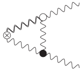
For ζ1j(1)(t)superscriptsubscript𝜁1𝑗1𝑡\zeta_{1j}^{(1)}(t), diagrams A03, A04, A05, A06, A07, A08, A09, A11, A13, A14, A15, A16, and A19 in Figs. 1630 contribute.151515Diagrams A10, A12, A17 (where the dotted line represents the ghost propagator), and A18 in these figures correspond to the conventional wave function renormalization and should be omitted in computing the operator mixing. In these and following diagrams, the cross generically represents one of composite operators in Eqs. (4.1)–(4.7) [in the present case, 𝒪~1μν(t,x)subscript~𝒪1𝜇𝜈𝑡𝑥\tilde{\mathcal{O}}_{1\mu\nu}(t,x)]. Apart from A19, we can borrow the results from Ref. Suzuki:2013gza for these diagrams. For completeness, these results are reproduced in the present convention in Table 5 of Appendix C. Combined with the contribution of diagram A19, we have

ζ11(1)(t)superscriptsubscript𝜁111𝑡\displaystyle\zeta_{11}^{(1)}(t) =g02(4π)2C2(G)[113ϵ(t)1+73],absentsuperscriptsubscript𝑔02superscript4𝜋2subscript𝐶2𝐺delimited-[]113italic-ϵsuperscript𝑡173\displaystyle=\frac{g_{0}^{2}}{(4\pi)^{2}}C_{2}(G)\left[\frac{11}{3}\epsilon(t)^{-1}+\frac{7}{3}\right], (4.36)
ζ12(1)(t)superscriptsubscript𝜁121𝑡\displaystyle\zeta_{12}^{(1)}(t) =g02(4π)2C2(G)[1112ϵ(t)116],absentsuperscriptsubscript𝑔02superscript4𝜋2subscript𝐶2𝐺delimited-[]1112italic-ϵsuperscript𝑡116\displaystyle=\frac{g_{0}^{2}}{(4\pi)^{2}}C_{2}(G)\left[-\frac{11}{12}\epsilon(t)^{-1}-\frac{1}{6}\right], (4.37)
ζ13(1)(t)superscriptsubscript𝜁131𝑡\displaystyle\zeta_{13}^{(1)}(t) =g04(4π)2C2(R)[23ϵ(t)1718],absentsuperscriptsubscript𝑔04superscript4𝜋2subscript𝐶2𝑅delimited-[]23italic-ϵsuperscript𝑡1718\displaystyle=\frac{g_{0}^{4}}{(4\pi)^{2}}C_{2}(R)\left[-\frac{2}{3}\epsilon(t)^{-1}-\frac{7}{18}\right], (4.38)
ζ14(1)(t)superscriptsubscript𝜁141𝑡\displaystyle\zeta_{14}^{(1)}(t) =g04(4π)2C2(R)[13ϵ(t)1718],absentsuperscriptsubscript𝑔04superscript4𝜋2subscript𝐶2𝑅delimited-[]13italic-ϵsuperscript𝑡1718\displaystyle=\frac{g_{0}^{4}}{(4\pi)^{2}}C_{2}(R)\left[\frac{1}{3}\epsilon(t)^{-1}-\frac{7}{18}\right], (4.39)
ζ15(1)(t)superscriptsubscript𝜁151𝑡\displaystyle\zeta_{15}^{(1)}(t) =g04(4π)2C2(R)[3ϵ(t)1+52],absentsuperscriptsubscript𝑔04superscript4𝜋2subscript𝐶2𝑅delimited-[]3italic-ϵsuperscript𝑡152\displaystyle=\frac{g_{0}^{4}}{(4\pi)^{2}}C_{2}(R)\left[3\epsilon(t)^{-1}+\frac{5}{2}\right], (4.40)

where

ϵ(t)11ϵ+ln(8πt).italic-ϵsuperscript𝑡11italic-ϵ8𝜋𝑡\epsilon(t)^{-1}\equiv\frac{1}{\epsilon}+\ln(8\pi t). (4.41)

By considering the trace part of 𝒪~1μνsubscript~𝒪1𝜇𝜈\tilde{\mathcal{O}}_{1\mu\nu}, from these we further have

ζ21(1)(t)superscriptsubscript𝜁211𝑡\displaystyle\zeta_{21}^{(1)}(t) =0,absent0\displaystyle=0, (4.42)
ζ22(1)(t)superscriptsubscript𝜁221𝑡\displaystyle\zeta_{22}^{(1)}(t) =ζ11(1)(t)+ζ12(1)(t)(42ϵ)=g02(4π)2C2(G)72,absentsuperscriptsubscript𝜁111𝑡superscriptsubscript𝜁121𝑡42italic-ϵsuperscriptsubscript𝑔02superscript4𝜋2subscript𝐶2𝐺72\displaystyle=\zeta_{11}^{(1)}(t)+\zeta_{12}^{(1)}(t)(4-2\epsilon)=\frac{g_{0}^{2}}{(4\pi)^{2}}C_{2}(G)\frac{7}{2}, (4.43)
ζ23(1)(t)superscriptsubscript𝜁231𝑡\displaystyle\zeta_{23}^{(1)}(t) =0,absent0\displaystyle=0, (4.44)
ζ24(1)(t)superscriptsubscript𝜁241𝑡\displaystyle\zeta_{24}^{(1)}(t) =2ζ13(1)(t)+ζ14(1)(t)(42ϵ)=g04(4π)2C2(R)(3),absent2superscriptsubscript𝜁131𝑡superscriptsubscript𝜁141𝑡42italic-ϵsuperscriptsubscript𝑔04superscript4𝜋2subscript𝐶2𝑅3\displaystyle=2\zeta_{13}^{(1)}(t)+\zeta_{14}^{(1)}(t)(4-2\epsilon)=\frac{g_{0}^{4}}{(4\pi)^{2}}C_{2}(R)(-3), (4.45)
ζ25(1)(t)superscriptsubscript𝜁251𝑡\displaystyle\zeta_{25}^{(1)}(t) =ζ15(1)(t)(42ϵ)=g04(4π)2C2(R)[12ϵ(t)1+4].absentsuperscriptsubscript𝜁151𝑡42italic-ϵsuperscriptsubscript𝑔04superscript4𝜋2subscript𝐶2𝑅delimited-[]12italic-ϵsuperscript𝑡14\displaystyle=\zeta_{15}^{(1)}(t)(4-2\epsilon)=\frac{g_{0}^{4}}{(4\pi)^{2}}C_{2}(R)\left[12\epsilon(t)^{-1}+4\right]. (4.46)
Refer to caption
Figure 31: B03
Refer to caption
Figure 32: B04
Refer to caption
Figure 33: B05
Refer to caption
Figure 34: B06
Refer to caption
Figure 35: B07
Refer to caption
Figure 36: B08
Refer to caption
Figure 37: B09
Refer to caption
Figure 38: B10
Refer to caption
Figure 39: B11
Refer to caption
Figure 40: B12
Refer to caption
Figure 41: B13
Refer to caption
Figure 42: B14
Refer to caption
Figure 43: B15
Refer to caption
Figure 44: B16
Refer to caption
Figure 45: B17
Refer to caption
Figure 46: B18

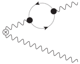
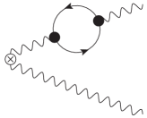
For ζ3j(1)(t)superscriptsubscript𝜁3𝑗1𝑡\zeta_{3j}^{(1)}(t) with j=1𝑗1j=1 and 222, diagrams B03, B04, B08, B09, B10, B11, and B12 in Figs. 3342 contribute. The contribution of each diagram is tabulated in Table 2. For ζ3j(1)(t)superscriptsubscript𝜁3𝑗1𝑡\zeta_{3j}^{(1)}(t) with j=3𝑗3j=3, 444, and 555, diagrams B06, B07, B13, B14, B15, B16, B17, and B18 in Figs. 3646 contribute and their contributions are tabulated in Table 3.

Table 2: ζ3j(1)superscriptsubscript𝜁3𝑗1\zeta_{3j}^{(1)} in units of 1(4π)2T(R)Nf1superscript4𝜋2𝑇𝑅subscript𝑁f\frac{1}{(4\pi)^{2}}T(R)N_{\mathrm{f}}
      diagram       ζ31(1)(t)superscriptsubscript𝜁311𝑡\zeta_{31}^{(1)}(t)       ζ32(1)(t)superscriptsubscript𝜁321𝑡\zeta_{32}^{(1)}(t)
      B03       163ϵ(t)1649163italic-ϵsuperscript𝑡1649-\dfrac{16}{3}\epsilon(t)^{-1}-\dfrac{64}{9}       43ϵ(t)1+25943italic-ϵsuperscript𝑡1259\dfrac{4}{3}\epsilon(t)^{-1}+\dfrac{25}{9}
      B04       00       00
      B08       00       1313-\dfrac{1}{3}
      B09       512512-\dfrac{5}{12}       2314423144-\dfrac{23}{144}
      B10       512512\dfrac{5}{12}       116116-\dfrac{1}{16}
      B11       109109\dfrac{10}{9}       7979\dfrac{7}{9}
      B12       00       00
Table 3: ζ3j(1)superscriptsubscript𝜁3𝑗1\zeta_{3j}^{(1)} in units of g02(4π)2C2(R)superscriptsubscript𝑔02superscript4𝜋2subscript𝐶2𝑅\frac{g_{0}^{2}}{(4\pi)^{2}}C_{2}(R)
      diagram       ζ33(1)(t)superscriptsubscript𝜁331𝑡\zeta_{33}^{(1)}(t)       ζ34(1)(t)superscriptsubscript𝜁341𝑡\zeta_{34}^{(1)}(t)       ζ35(1)(t)superscriptsubscript𝜁351𝑡\zeta_{35}^{(1)}(t)
      B06       13ϵ(t)1+11813italic-ϵsuperscript𝑡1118-\dfrac{1}{3}\epsilon(t)^{-1}+\dfrac{1}{18}       23ϵ(t)1+5923italic-ϵsuperscript𝑡159\dfrac{2}{3}\epsilon(t)^{-1}+\dfrac{5}{9}       8ϵ(t)1+88italic-ϵsuperscript𝑡188\epsilon(t)^{-1}+8
      B07       2ϵ(t)1+22italic-ϵsuperscript𝑡122\epsilon(t)^{-1}+2       2ϵ(t)122italic-ϵsuperscript𝑡12-2\epsilon(t)^{-1}-2       8ϵ(t)188italic-ϵsuperscript𝑡18-8\epsilon(t)^{-1}-8
      B13       00       111       00
      B14       00       00       00
      B15       2ϵ(t)1+22italic-ϵsuperscript𝑡122\epsilon(t)^{-1}+2       00       00
      B16       00       00       00
      B17       22-2       00       00
      B18       4ϵ(t)124italic-ϵsuperscript𝑡12-4\epsilon(t)^{-1}-2       00       00

As the sum of these contributions, we have

ζ31(1)(t)superscriptsubscript𝜁311𝑡\displaystyle\zeta_{31}^{(1)}(t) =1(4π)2T(R)Nf[163ϵ(t)16],absent1superscript4𝜋2𝑇𝑅subscript𝑁fdelimited-[]163italic-ϵsuperscript𝑡16\displaystyle=\frac{1}{(4\pi)^{2}}T(R)N_{\mathrm{f}}\left[-\frac{16}{3}\epsilon(t)^{-1}-6\right], (4.47)
ζ32(1)(t)superscriptsubscript𝜁321𝑡\displaystyle\zeta_{32}^{(1)}(t) =1(4π)2T(R)Nf[43ϵ(t)1+3],absent1superscript4𝜋2𝑇𝑅subscript𝑁fdelimited-[]43italic-ϵsuperscript𝑡13\displaystyle=\frac{1}{(4\pi)^{2}}T(R)N_{\mathrm{f}}\left[\frac{4}{3}\epsilon(t)^{-1}+3\right], (4.48)
ζ33(1)(t)superscriptsubscript𝜁331𝑡\displaystyle\zeta_{33}^{(1)}(t) =g2(4π)2C2(R)[31ϵΦ(t)]+g02(4π)2C2(R)[13ϵ(t)1+118],absentsuperscript𝑔2superscript4𝜋2subscript𝐶2𝑅delimited-[]31italic-ϵΦ𝑡superscriptsubscript𝑔02superscript4𝜋2subscript𝐶2𝑅delimited-[]13italic-ϵsuperscript𝑡1118\displaystyle=\frac{g^{2}}{(4\pi)^{2}}C_{2}(R)\left[3\frac{1}{\epsilon}-\Phi(t)\right]+\frac{g_{0}^{2}}{(4\pi)^{2}}C_{2}(R)\left[-\frac{1}{3}\epsilon(t)^{-1}+\frac{1}{18}\right], (4.49)
ζ34(1)(t)superscriptsubscript𝜁341𝑡\displaystyle\zeta_{34}^{(1)}(t) =g02(4π)2C2(R)[43ϵ(t)149],absentsuperscriptsubscript𝑔02superscript4𝜋2subscript𝐶2𝑅delimited-[]43italic-ϵsuperscript𝑡149\displaystyle=\frac{g_{0}^{2}}{(4\pi)^{2}}C_{2}(R)\left[-\frac{4}{3}\epsilon(t)^{-1}-\frac{4}{9}\right], (4.50)
ζ35(1)(t)superscriptsubscript𝜁351𝑡\displaystyle\zeta_{35}^{(1)}(t) =0,absent0\displaystyle=0, (4.51)

where in ζ33(1)(t)superscriptsubscript𝜁331𝑡\zeta_{33}^{(1)}(t) (4.49) the first term in the right-hand side comes from the conversion from the un-ringed fields to the ringed fields in Eqs. (3.22) and (3.25)—recall Eq. (3.32); the combination Φ(t)Φ𝑡\Phi(t) is given by Eq. (3.34). From these, we further have

ζ41(1)(t)superscriptsubscript𝜁411𝑡\displaystyle\zeta_{41}^{(1)}(t) =0,absent0\displaystyle=0, (4.52)
ζ42(1)(t)superscriptsubscript𝜁421𝑡\displaystyle\zeta_{42}^{(1)}(t) =12ζ31(1)(t)+12ζ32(1)(t)(42ϵ)=1(4π)2T(R)Nf53,absent12superscriptsubscript𝜁311𝑡12superscriptsubscript𝜁321𝑡42italic-ϵ1superscript4𝜋2𝑇𝑅subscript𝑁f53\displaystyle=\frac{1}{2}\zeta_{31}^{(1)}(t)+\frac{1}{2}\zeta_{32}^{(1)}(t)(4-2\epsilon)=\frac{1}{(4\pi)^{2}}T(R)N_{\mathrm{f}}\frac{5}{3}, (4.53)
ζ43(1)(t)superscriptsubscript𝜁431𝑡\displaystyle\zeta_{43}^{(1)}(t) =0,absent0\displaystyle=0, (4.54)
ζ44(1)(t)superscriptsubscript𝜁441𝑡\displaystyle\zeta_{44}^{(1)}(t) =ζ33(1)(t)+12ζ34(1)(t)(42ϵ)absentsuperscriptsubscript𝜁331𝑡12superscriptsubscript𝜁341𝑡42italic-ϵ\displaystyle=\zeta_{33}^{(1)}(t)+\frac{1}{2}\zeta_{34}^{(1)}(t)(4-2\epsilon)
=g2(4π)2C2(R)[31ϵΦ(t)]+g02(4π)2C2(R)[3ϵ(t)1+12],absentsuperscript𝑔2superscript4𝜋2subscript𝐶2𝑅delimited-[]31italic-ϵΦ𝑡superscriptsubscript𝑔02superscript4𝜋2subscript𝐶2𝑅delimited-[]3italic-ϵsuperscript𝑡112\displaystyle=\frac{g^{2}}{(4\pi)^{2}}C_{2}(R)\left[3\frac{1}{\epsilon}-\Phi(t)\right]+\frac{g_{0}^{2}}{(4\pi)^{2}}C_{2}(R)\left[-3\epsilon(t)^{-1}+\frac{1}{2}\right], (4.55)
ζ45(1)(t)superscriptsubscript𝜁451𝑡\displaystyle\zeta_{45}^{(1)}(t) =0.absent0\displaystyle=0. (4.56)

Finally,

ζ51(1)(t)=ζ52(1)(t)=ζ53(1)(t)=ζ54(1)(t)=0,superscriptsubscript𝜁511𝑡superscriptsubscript𝜁521𝑡superscriptsubscript𝜁531𝑡superscriptsubscript𝜁541𝑡0\zeta_{51}^{(1)}(t)=\zeta_{52}^{(1)}(t)=\zeta_{53}^{(1)}(t)=\zeta_{54}^{(1)}(t)=0, (4.57)

and ζ55(1)(t)superscriptsubscript𝜁551𝑡\zeta_{55}^{(1)}(t) is given by the sum of the contributions of one-loop diagrams in Table 4 and the conversion factor to the ringed fields:

Table 4: ζ55(1)(t)superscriptsubscript𝜁551𝑡\zeta_{55}^{(1)}(t) in units of g02(4π)2C2(R)superscriptsubscript𝑔02superscript4𝜋2subscript𝐶2𝑅\frac{g_{0}^{2}}{(4\pi)^{2}}C_{2}(R).
      diagram       ζ55(1)(t)superscriptsubscript𝜁551𝑡\zeta_{55}^{(1)}(t)
      B06       4ϵ(t)124italic-ϵsuperscript𝑡12-4\epsilon(t)^{-1}-2
      B13       00
      B14       00
      B15       2ϵ(t)1+22italic-ϵsuperscript𝑡122\epsilon(t)^{-1}+2
      B16       00
      B18       4ϵ(t)124italic-ϵsuperscript𝑡12-4\epsilon(t)^{-1}-2
ζ55(1)(t)=g2(4π)2C2(R)[61ϵΦ(t)]+g02(4π)2C2(R)[6ϵ(t)12].superscriptsubscript𝜁551𝑡superscript𝑔2superscript4𝜋2subscript𝐶2𝑅delimited-[]61italic-ϵΦ𝑡superscriptsubscript𝑔02superscript4𝜋2subscript𝐶2𝑅delimited-[]6italic-ϵsuperscript𝑡12\displaystyle\zeta_{55}^{(1)}(t)=\frac{g^{2}}{(4\pi)^{2}}C_{2}(R)\left[6\frac{1}{\epsilon}-\Phi(t)\right]+\frac{g_{0}^{2}}{(4\pi)^{2}}C_{2}(R)\left[-6\epsilon(t)^{-1}-2\right]. (4.58)

We have now obtained all ζij(1)(t)superscriptsubscript𝜁𝑖𝑗1𝑡\zeta_{ij}^{(1)}(t) in Eqs. (4.28) and (4.29). Then, since the matrix ζij(t)subscript𝜁𝑖𝑗𝑡\zeta_{ij}(t) in the tree-level approximation is a unit matrix, it is straightforward to invert the matrix ζij(t)subscript𝜁𝑖𝑗𝑡\zeta_{ij}(t) in the one-loop approximation; Eqs. (4.19) and (4.20) thus yield

c1(t)subscript𝑐1𝑡\displaystyle c_{1}(t) =1g02[1ζ11(1)(t)]14ζ31(1)(t),absent1superscriptsubscript𝑔02delimited-[]1superscriptsubscript𝜁111𝑡14superscriptsubscript𝜁311𝑡\displaystyle=\frac{1}{g_{0}^{2}}\left[1-\zeta_{11}^{(1)}(t)\right]-\frac{1}{4}\zeta_{31}^{(1)}(t), (4.59)
c2(t)subscript𝑐2𝑡\displaystyle c_{2}(t) =1g02(12ϵ)ζ12(1)(t)+(3412ϵ)ζ32(1)(t)+316ζ31(1)(t),absent1superscriptsubscript𝑔0212italic-ϵsuperscriptsubscript𝜁121𝑡3412italic-ϵsuperscriptsubscript𝜁321𝑡316superscriptsubscript𝜁311𝑡\displaystyle=\frac{1}{g_{0}^{2}}\left(-\frac{1}{2}\epsilon\right)\zeta_{12}^{(1)}(t)+\left(\frac{3}{4}-\frac{1}{2}\epsilon\right)\zeta_{32}^{(1)}(t)+\frac{3}{16}\zeta_{31}^{(1)}(t), (4.60)
c3(t)subscript𝑐3𝑡\displaystyle c_{3}(t) ={1g02[ζ13(1)(t)]+1414ζ33(1)(t)}Z(ϵ)1,absent1superscriptsubscript𝑔02delimited-[]superscriptsubscript𝜁131𝑡1414superscriptsubscript𝜁331𝑡𝑍superscriptitalic-ϵ1\displaystyle=\left\{\frac{1}{g_{0}^{2}}\left[-\zeta_{13}^{(1)}(t)\right]+\frac{1}{4}-\frac{1}{4}\zeta_{33}^{(1)}(t)\right\}Z(\epsilon)^{-1}, (4.61)
c4(t)subscript𝑐4𝑡\displaystyle c_{4}(t) ={1g02[12ϵζ14(1)(t)32ζ13(1)(t)]+(3412ϵ)ζ34(1)(t)}Z(ϵ)1,absent1superscriptsubscript𝑔02delimited-[]12italic-ϵsuperscriptsubscript𝜁141𝑡32superscriptsubscript𝜁131𝑡3412italic-ϵsuperscriptsubscript𝜁341𝑡𝑍superscriptitalic-ϵ1\displaystyle=\left\{\frac{1}{g_{0}^{2}}\left[-\frac{1}{2}\epsilon\zeta_{14}^{(1)}(t)-\frac{3}{2}\zeta_{13}^{(1)}(t)\right]+\left(\frac{3}{4}-\frac{1}{2}\epsilon\right)\zeta_{34}^{(1)}(t)\right\}Z(\epsilon)^{-1}, (4.62)
c5(t)subscript𝑐5𝑡\displaystyle c_{5}(t) ={1g02[12ϵζ15(1)(t)]1+ζ55(1)(t)}Z(ϵ)1.absent1superscriptsubscript𝑔02delimited-[]12italic-ϵsuperscriptsubscript𝜁151𝑡1superscriptsubscript𝜁551𝑡𝑍superscriptitalic-ϵ1\displaystyle=\left\{\frac{1}{g_{0}^{2}}\left[-\frac{1}{2}\epsilon\zeta_{15}^{(1)}(t)\right]-1+\zeta_{55}^{(1)}(t)\right\}Z(\epsilon)^{-1}. (4.63)

Then, by using the renormalized gauge coupling in the MS scheme (A.1), to the one-loop order, we have (for ϵ0italic-ϵ0\epsilon\to 0)

c1(t)subscript𝑐1𝑡\displaystyle c_{1}(t) =1g2b0ln(8πμ2t)1(4π)2[73C2(G)32T(R)Nf],absent1superscript𝑔2subscript𝑏08𝜋superscript𝜇2𝑡1superscript4𝜋2delimited-[]73subscript𝐶2𝐺32𝑇𝑅subscript𝑁f\displaystyle=\frac{1}{g^{2}}-b_{0}\ln(8\pi\mu^{2}t)-\frac{1}{(4\pi)^{2}}\left[\frac{7}{3}C_{2}(G)-\frac{3}{2}T(R)N_{\mathrm{f}}\right], (4.64)
c2(t)subscript𝑐2𝑡\displaystyle c_{2}(t) =181(4π)2[113C2(G)+113T(R)Nf],absent181superscript4𝜋2delimited-[]113subscript𝐶2𝐺113𝑇𝑅subscript𝑁f\displaystyle=\frac{1}{8}\frac{1}{(4\pi)^{2}}\left[\frac{11}{3}C_{2}(G)+\frac{11}{3}T(R)N_{\mathrm{f}}\right], (4.65)
c3(t)subscript𝑐3𝑡\displaystyle c_{3}(t) =14{1+g2(4π)2C2(R)[32+ln(432)]},absent141superscript𝑔2superscript4𝜋2subscript𝐶2𝑅delimited-[]32432\displaystyle=\frac{1}{4}\left\{1+\frac{g^{2}}{(4\pi)^{2}}C_{2}(R)\left[\frac{3}{2}+\ln(432)\right]\right\}, (4.66)
c4(t)subscript𝑐4𝑡\displaystyle c_{4}(t) =18d0g2,absent18subscript𝑑0superscript𝑔2\displaystyle=\frac{1}{8}d_{0}g^{2}, (4.67)
c5(t)subscript𝑐5𝑡\displaystyle c_{5}(t) ={1+g2(4π)2C2(R)[3ln(8πμ2t)+72+ln(432)]}.absent1superscript𝑔2superscript4𝜋2subscript𝐶2𝑅delimited-[]38𝜋superscript𝜇2𝑡72432\displaystyle=-\left\{1+\frac{g^{2}}{(4\pi)^{2}}C_{2}(R)\left[3\ln(8\pi\mu^{2}t)+\frac{7}{2}+\ln(432)\right]\right\}. (4.68)

Since the ci(t)subscript𝑐𝑖𝑡c_{i}(t) in Eq. (4.18) connect the finite energy–momentum tensor and UV-finite local products 𝒪~iμν(t,x)subscript~𝒪𝑖𝜇𝜈𝑡𝑥\tilde{\mathcal{O}}_{i\mu\nu}(t,x) constructed from (ringed) flowed fields, they should be UV finite. That our explicit one-loop calculation of ci(t)subscript𝑐𝑖𝑡c_{i}(t) confirms this finiteness is quite reassuring.

If one prefers the MS¯¯MS\overline{\text{MS}} scheme instead of the MS scheme assumed in above expressions, it suffices to make the replacement

μ2eγE4πμ2,superscript𝜇2superscriptesubscript𝛾E4𝜋superscript𝜇2\mu^{2}\to\frac{\mathrm{e}^{\gamma_{\mathrm{E}}}}{4\pi}\mu^{2}, (4.69)

where γEsubscript𝛾E\gamma_{\mathrm{E}} is Euler’s constant.

4.3 A consistency check: The trace anomaly

It is interesting to see that Eq. (4.18) with ci(t)subscript𝑐𝑖𝑡c_{i}(t) in Eqs. (4.64)–(4.68) in fact reproduces the trace anomaly (2.13) in the one-loop approximation. At first brief glance, c2(t)subscript𝑐2𝑡c_{2}(t) in Eq. (4.65) is incompatible with the correct trace anomaly, because δμν[𝒪~1μν(1/4)𝒪~2μν]=0subscript𝛿𝜇𝜈delimited-[]subscript~𝒪1𝜇𝜈14subscript~𝒪2𝜇𝜈0\delta_{\mu\nu}[\tilde{\mathcal{O}}_{1\mu\nu}-(1/4)\tilde{\mathcal{O}}_{2\mu\nu}]=0 for D=4𝐷4D=4 and δμν𝒪~2μν=4{FρσaFρσa}R(x)+O(g2)subscript𝛿𝜇𝜈subscript~𝒪2𝜇𝜈4subscriptsuperscriptsubscript𝐹𝜌𝜎𝑎superscriptsubscript𝐹𝜌𝜎𝑎𝑅𝑥𝑂superscript𝑔2\delta_{\mu\nu}\tilde{\mathcal{O}}_{2\mu\nu}=4\left\{F_{\rho\sigma}^{a}F_{\rho\sigma}^{a}\right\}_{R}(x)+O(g^{2}) [the last equality follows from Eq. (A.19)]. On the other hand, 4c2(t)4subscript𝑐2𝑡4c_{2}(t) from Eq. (4.65) is not identical to b0/2subscript𝑏02b_{0}/2, where b0subscript𝑏0b_{0} is the first coefficient of the beta function (2.18), the correct one-loop coefficient of the trace anomaly.

This is a premature judgment, however. In fact, ζ42(1)(t)superscriptsubscript𝜁421𝑡\zeta_{42}^{(1)}(t) in Eq. (4.53) shows that there exists an operator mixing of the form

χ¯̊(t,x)/Dχ̊(t,x)={ψ¯/Dψ}R(x)+1(4π)2T(R)Nf53{FρσaFρσa}R(x)+.̊¯𝜒𝑡𝑥/𝐷̊𝜒𝑡𝑥subscript¯𝜓/𝐷𝜓𝑅𝑥1superscript4𝜋2𝑇𝑅subscript𝑁f53subscriptsuperscriptsubscript𝐹𝜌𝜎𝑎superscriptsubscript𝐹𝜌𝜎𝑎𝑅𝑥\mathring{\bar{\chi}}(t,x)\overleftrightarrow{{\ooalign{\hfil/\hfil\crcr$D$}}}\mathring{\chi}(t,x)=\left\{\bar{\psi}\overleftrightarrow{{\ooalign{\hfil/\hfil\crcr$D$}}}\psi\right\}_{R}(x)+\frac{1}{(4\pi)^{2}}T(R)N_{\mathrm{f}}\frac{5}{3}\left\{F_{\rho\sigma}^{a}F_{\rho\sigma}^{a}\right\}_{R}(x)+\dotsb. (4.70)

Then the last term precisely fills the difference between 4c2(t)4subscript𝑐2𝑡4c_{2}(t) and b0/2subscript𝑏02b_{0}/2.

In this way, to the one-loop order, we have

δμν{Tμν}R(x)subscript𝛿𝜇𝜈subscriptsubscript𝑇𝜇𝜈𝑅𝑥\displaystyle\delta_{\mu\nu}\left\{T_{\mu\nu}\right\}_{R}(x) =121(4π)2[113C2(G)43T(R)Nf]{FρσaFρσa}R(x)absent121superscript4𝜋2delimited-[]113subscript𝐶2𝐺43𝑇𝑅subscript𝑁fsubscriptsuperscriptsubscript𝐹𝜌𝜎𝑎superscriptsubscript𝐹𝜌𝜎𝑎𝑅𝑥\displaystyle=\frac{1}{2}\frac{1}{(4\pi)^{2}}\left[\frac{11}{3}C_{2}(G)-\frac{4}{3}T(R)N_{\mathrm{f}}\right]\left\{F_{\rho\sigma}^{a}F_{\rho\sigma}^{a}\right\}_{R}(x)
32{ψ¯/Dψ}R(x)[4+g2(4π)26C2(R)]m{ψ¯ψ}R(x).32subscript¯𝜓/𝐷𝜓𝑅𝑥delimited-[]4superscript𝑔2superscript4𝜋26subscript𝐶2𝑅𝑚subscript¯𝜓𝜓𝑅𝑥\displaystyle\qquad{}-\frac{3}{2}\left\{\bar{\psi}\overleftrightarrow{{\ooalign{\hfil/\hfil\crcr$D$}}}\psi\right\}_{R}(x)-\left[4+\frac{g^{2}}{(4\pi)^{2}}6C_{2}(R)\right]m\left\{\bar{\psi}\psi\right\}_{R}(x). (4.73)

This reproduces the trace anomaly (2.13) in the one-loop level if one uses the equation of motion of renormalized field,

{ψ¯/Dψ}R(x)=2m{ψ¯ψ}R(x),subscript¯𝜓/𝐷𝜓𝑅𝑥2𝑚subscript¯𝜓𝜓𝑅𝑥\left\{\bar{\psi}\overleftrightarrow{{\ooalign{\hfil/\hfil\crcr$D$}}}\psi\right\}_{R}(x)=-2m\left\{\bar{\psi}\psi\right\}_{R}(x), (4.74)

whose use is justified when there is no other operator in the point x𝑥x as we are assuming. We observe that our one-loop result in Eqs. (4.64)–(4.68) is consistent with the trace anomaly.

In Ref. Suzuki:2013gza , for the pure Yang–Mills theory, the next-to-leading (two-loop order) term in c2(t)subscript𝑐2𝑡c_{2}(t) was determined as

c2(t)=18b018b0[1(4π)2G2(G)72b1b0]g2,subscript𝑐2𝑡18subscript𝑏018subscript𝑏0delimited-[]1superscript4𝜋2subscript𝐺2𝐺72subscript𝑏1subscript𝑏0superscript𝑔2c_{2}(t)=\frac{1}{8}b_{0}-\frac{1}{8}b_{0}\left[\frac{1}{(4\pi)^{2}}G_{2}(G)\frac{7}{2}-\frac{b_{1}}{b_{0}}\right]g^{2}, (4.75)

where b0=[1/(4π)2](11/3)C2(G)subscript𝑏0delimited-[]1superscript4𝜋2113subscript𝐶2𝐺b_{0}=[1/(4\pi)^{2}](11/3)C_{2}(G) and b1=[1/(4π)4](34/3)C2(G)2subscript𝑏1delimited-[]1superscript4𝜋4343subscript𝐶2superscript𝐺2b_{1}=[1/(4\pi)^{4}](34/3)C_{2}(G)^{2}, by imposing that the expression (4.18) reproduces the trace anomaly (2.13) to the two-loop order. For the present system with fermions, however, it seems that this requirement alone cannot fix the next-to-leading terms in c2(t)subscript𝑐2𝑡c_{2}(t) and in c4(t)subscript𝑐4𝑡c_{4}(t); so we are content with the one-loop formulas, Eqs. (4.64)–(4.68), in the present paper treating a system containing fermions.

4.4 Master formula

From Eq. (4.18), the energy–momentum tensor is given by the t0𝑡0t\to 0 limit,

{Tμν}R(x)subscriptsubscript𝑇𝜇𝜈𝑅𝑥\displaystyle\left\{T_{\mu\nu}\right\}_{R}(x) =limt0{c1(t)[𝒪~1μν(t,x)14𝒪~2μν(t,x)]\displaystyle=\lim_{t\to 0}\biggl{\{}c_{1}(t)\left[\tilde{\mathcal{O}}_{1\mu\nu}(t,x)-\frac{1}{4}\tilde{\mathcal{O}}_{2\mu\nu}(t,x)\right]
+c2(t)[𝒪~2μν(t,x)𝒪~2μν(t,x)]subscript𝑐2𝑡delimited-[]subscript~𝒪2𝜇𝜈𝑡𝑥delimited-⟨⟩subscript~𝒪2𝜇𝜈𝑡𝑥\displaystyle\qquad\qquad{}+c_{2}(t)\left[\tilde{\mathcal{O}}_{2\mu\nu}(t,x)-\left\langle\tilde{\mathcal{O}}_{2\mu\nu}(t,x)\right\rangle\right]
+c3(t)[𝒪~3μν(t,x)2𝒪~4μν(t,x)𝒪~3μν(t,x)2𝒪~4μν(t,x)]subscript𝑐3𝑡delimited-[]subscript~𝒪3𝜇𝜈𝑡𝑥2subscript~𝒪4𝜇𝜈𝑡𝑥delimited-⟨⟩subscript~𝒪3𝜇𝜈𝑡𝑥2subscript~𝒪4𝜇𝜈𝑡𝑥\displaystyle\qquad\qquad\qquad{}+c_{3}(t)\left[\tilde{\mathcal{O}}_{3\mu\nu}(t,x)-2\tilde{\mathcal{O}}_{4\mu\nu}(t,x)-\left\langle\tilde{\mathcal{O}}_{3\mu\nu}(t,x)-2\tilde{\mathcal{O}}_{4\mu\nu}(t,x)\right\rangle\right]
+c4(t)[𝒪~4μν(t,x)𝒪~4μν(t,x)]subscript𝑐4𝑡delimited-[]subscript~𝒪4𝜇𝜈𝑡𝑥delimited-⟨⟩subscript~𝒪4𝜇𝜈𝑡𝑥\displaystyle\qquad\qquad\qquad\qquad{}+c_{4}(t)\left[\tilde{\mathcal{O}}_{4\mu\nu}(t,x)-\left\langle\tilde{\mathcal{O}}_{4\mu\nu}(t,x)\right\rangle\right]
+c5(t)[𝒪~5μν(t,x)𝒪~5μν(t,x)]},\displaystyle\qquad\qquad\qquad\qquad\qquad{}+c_{5}(t)\left[\tilde{\mathcal{O}}_{5\mu\nu}(t,x)-\left\langle\tilde{\mathcal{O}}_{5\mu\nu}(t,x)\right\rangle\right]\biggr{\}}, (4.76)

where operators in the right-hand side are given by Eqs. (4.1)–(4.7). One may further use the identities

2𝒪~3μν(t,x)=𝒪~4μν(t,x)=2dim(R)Nf(4π)2t2δμν2delimited-⟨⟩subscript~𝒪3𝜇𝜈𝑡𝑥delimited-⟨⟩subscript~𝒪4𝜇𝜈𝑡𝑥2dimension𝑅subscript𝑁fsuperscript4𝜋2superscript𝑡2subscript𝛿𝜇𝜈2\left\langle\tilde{\mathcal{O}}_{3\mu\nu}(t,x)\right\rangle=\left\langle\tilde{\mathcal{O}}_{4\mu\nu}(t,x)\right\rangle=\frac{-2\dim(R)N_{\mathrm{f}}}{(4\pi)^{2}t^{2}}\delta_{\mu\nu} (4.77)

to make the expression a little simpler. Applying the consequence of the renormalization group argument, Eqs. (4.26)–(4.27), to Eqs. (4.64)–(4.68), we have

c1(t)subscript𝑐1𝑡\displaystyle c_{1}(t) =1g¯(1/8t)2b0lnπ1(4π)2[73C2(G)32T(R)Nf],absent1¯𝑔superscript18𝑡2subscript𝑏0𝜋1superscript4𝜋2delimited-[]73subscript𝐶2𝐺32𝑇𝑅subscript𝑁f\displaystyle=\frac{1}{\bar{g}(1/\sqrt{8t})^{2}}-b_{0}\ln\pi-\frac{1}{(4\pi)^{2}}\left[\frac{7}{3}C_{2}(G)-\frac{3}{2}T(R)N_{\mathrm{f}}\right], (4.78)
c2(t)subscript𝑐2𝑡\displaystyle c_{2}(t) =181(4π)2[113C2(G)+113T(R)Nf],absent181superscript4𝜋2delimited-[]113subscript𝐶2𝐺113𝑇𝑅subscript𝑁f\displaystyle=\frac{1}{8}\frac{1}{(4\pi)^{2}}\left[\frac{11}{3}C_{2}(G)+\frac{11}{3}T(R)N_{\mathrm{f}}\right], (4.79)
c3(t)subscript𝑐3𝑡\displaystyle c_{3}(t) =14{1+g¯(1/8t)2(4π)2C2(R)[32+ln(432)]},absent141¯𝑔superscript18𝑡2superscript4𝜋2subscript𝐶2𝑅delimited-[]32432\displaystyle=\frac{1}{4}\left\{1+\frac{\bar{g}(1/\sqrt{8t})^{2}}{(4\pi)^{2}}C_{2}(R)\left[\frac{3}{2}+\ln(432)\right]\right\}, (4.80)
c4(t)subscript𝑐4𝑡\displaystyle c_{4}(t) =18d0g¯(1/8t)2,absent18subscript𝑑0¯𝑔superscript18𝑡2\displaystyle=\frac{1}{8}d_{0}\bar{g}(1/\sqrt{8t})^{2}, (4.81)
c5(t)subscript𝑐5𝑡\displaystyle c_{5}(t) =m¯(1/8t)m{1+g¯(1/8t)2(4π)2C2(R)[3lnπ+72+ln(432)]},absent¯𝑚18𝑡𝑚1¯𝑔superscript18𝑡2superscript4𝜋2subscript𝐶2𝑅delimited-[]3𝜋72432\displaystyle=-\frac{\bar{m}(1/\sqrt{8t})}{m}\left\{1+\frac{\bar{g}(1/\sqrt{8t})^{2}}{(4\pi)^{2}}C_{2}(R)\left[3\ln\pi+\frac{7}{2}+\ln(432)\right]\right\}, (4.82)

where g¯(q)¯𝑔𝑞\bar{g}(q) is the running gauge coupling in the MS scheme. For going from the MS scheme to the MS¯¯MS\overline{\text{MS}} scheme, it suffices to make the following replacement corresponding to Eq. (4.69),

lnπγE2ln2,𝜋subscript𝛾E22\ln\pi\to\gamma_{\mathrm{E}}-2\ln 2, (4.83)

in the above expressions. Equation (4.76) with Eqs. (4.78)–(4.82) is our main result. Note that the renormalized mass parameter m𝑚m in c5(t)subscript𝑐5𝑡c_{5}(t) (4.82) and that in 𝒪~5μν(t,x)subscript~𝒪5𝜇𝜈𝑡𝑥\tilde{\mathcal{O}}_{5\mu\nu}(t,x) (4.7) are redundant in Eq. (4.76) because they are cancelled out in the product. For the running mass parameter m¯(1/8t)¯𝑚18𝑡\bar{m}(1/\sqrt{8t}) in c5(t)subscript𝑐5𝑡c_{5}(t) for t0𝑡0t\to 0, one may use the relation

m¯(q)¯𝑚𝑞\displaystyle\bar{m}(q) =[2b0g¯(q)2]d0/2b0exp{0g¯(q)dg[γm(g)β(g)d0b0g]}mabsentsuperscriptdelimited-[]2subscript𝑏0¯𝑔superscript𝑞2subscript𝑑02subscript𝑏0superscriptsubscript0¯𝑔𝑞differential-d𝑔delimited-[]subscript𝛾𝑚𝑔𝛽𝑔subscript𝑑0subscript𝑏0𝑔superscript𝑚\displaystyle=[2b_{0}\bar{g}(q)^{2}]^{d_{0}/2b_{0}}\exp\left\{\int_{0}^{\bar{g}(q)}\mathrm{d}g\,\left[-\frac{\gamma_{m}(g)}{\beta(g)}-\frac{d_{0}}{b_{0}g}\right]\right\}m^{\infty}
=(2)d0/2b0[1d0b12b03(1+ln)+d12b02+O(2)]m,ln(q2/Λ2),formulae-sequenceabsentsuperscript2subscript𝑑02subscript𝑏0delimited-[]1subscript𝑑0subscript𝑏12superscriptsubscript𝑏031subscript𝑑12superscriptsubscript𝑏02𝑂superscript2superscript𝑚superscript𝑞2superscriptΛ2\displaystyle=\left(\frac{2}{\ell}\right)^{d_{0}/2b_{0}}\left[1-\frac{d_{0}b_{1}}{2b_{0}^{3}\ell}(1+\ln\ell)+\frac{d_{1}}{2b_{0}^{2}\ell}+O(\ell^{-2})\right]m^{\infty},\qquad\ell\equiv\ln(q^{2}/\Lambda^{2}), (4.84)

where msuperscript𝑚m^{\infty} denotes the renormalization group invariant mass. For the massive fermion, msuperscript𝑚m^{\infty} may be determined by using the method established in Ref. Capitani:1998mq , for example. For the massless fermion, m=0superscript𝑚0m^{\infty}=0 and we can simply discard the last line of Eq. (4.76).

5 Equation of motion in the small flow-time limit

Let us consider the following representations for small flow-time:

δμν[ψ¯(x)/Dψ(x)+2m0ψ¯(x)ψ(x)]subscript𝛿𝜇𝜈delimited-[]¯𝜓𝑥/𝐷𝜓𝑥2subscript𝑚0¯𝜓𝑥𝜓𝑥\displaystyle\delta_{\mu\nu}\left[\bar{\psi}(x)\overleftrightarrow{{\ooalign{\hfil/\hfil\crcr$D$}}}\psi(x)+2m_{0}\bar{\psi}(x)\psi(x)\right] (5.3)
=d2(t)𝒪~2μν(t,x)+d4(t)𝒪~4μν(t,x)+d5(t)𝒪~5μν+O(t),absentsubscript𝑑2𝑡subscript~𝒪2𝜇𝜈𝑡𝑥subscript𝑑4𝑡subscript~𝒪4𝜇𝜈𝑡𝑥subscript𝑑5𝑡subscript~𝒪5𝜇𝜈𝑂𝑡\displaystyle=d_{2}(t)\tilde{\mathcal{O}}_{2\mu\nu}(t,x)+d_{4}(t)\tilde{\mathcal{O}}_{4\mu\nu}(t,x)+d_{5}(t)\tilde{\mathcal{O}}_{5\mu\nu}+O(t), (5.4)

and

δμνm0ψ¯(x)ψ(x)=e5(t)𝒪~5μν(t,x)+O(t),subscript𝛿𝜇𝜈subscript𝑚0¯𝜓𝑥𝜓𝑥subscript𝑒5𝑡subscript~𝒪5𝜇𝜈𝑡𝑥𝑂𝑡\delta_{\mu\nu}m_{0}\bar{\psi}(x)\psi(x)=e_{5}(t)\tilde{\mathcal{O}}_{5\mu\nu}(t,x)+O(t), (5.5)

where it is understood that the vacuum expectation values are subtracted on both sides of the equations. By a renormalization group argument identical to that which led to Eqs. (4.26) and (4.27) and the one-loop calculation in Sect. 4, for t0𝑡0t\to 0 we have

d2(t)subscript𝑑2𝑡\displaystyle d_{2}(t) =1(4π)2T(R)Nf53,absent1superscript4𝜋2𝑇𝑅subscript𝑁f53\displaystyle=-\frac{1}{(4\pi)^{2}}T(R)N_{\mathrm{f}}\frac{5}{3}, (5.6)
d4(t)subscript𝑑4𝑡\displaystyle d_{4}(t) =1+g¯(1/8t)2(4π)2C2(R)[12+ln(432)],absent1¯𝑔superscript18𝑡2superscript4𝜋2subscript𝐶2𝑅delimited-[]12432\displaystyle=1+\frac{\bar{g}(1/\sqrt{8t})^{2}}{(4\pi)^{2}}C_{2}(R)\left[-\frac{1}{2}+\ln(432)\right], (5.7)
d5(t)subscript𝑑5𝑡\displaystyle d_{5}(t) =m¯(1/8t)m2{1+g¯(1/8t)2(4π)2C2(R)[3lnπ+2+ln(432)]},absent¯𝑚18𝑡𝑚21¯𝑔superscript18𝑡2superscript4𝜋2subscript𝐶2𝑅delimited-[]3𝜋2432\displaystyle=\frac{\bar{m}(1/\sqrt{8t})}{m}2\left\{1+\frac{\bar{g}(1/\sqrt{8t})^{2}}{(4\pi)^{2}}C_{2}(R)\left[3\ln\pi+2+\ln(432)\right]\right\}, (5.8)

and e5(t)=(1/2)d5(t)subscript𝑒5𝑡12subscript𝑑5𝑡e_{5}(t)=(1/2)d_{5}(t). We note that since the left-hand side of Eq. (5.4) is proportional to the equation of motion of the fermion field, when the position x𝑥x does not coincide with positions of other operators in the position space, we may set the combination to zero (the Schwinger–Dyson equation). This implies that we can make the replacement (the subtraction of the vacuum expectation value is understood)

𝒪~4μν(t,x)subscript~𝒪4𝜇𝜈𝑡𝑥\displaystyle\tilde{\mathcal{O}}_{4\mu\nu}(t,x) 1(4π)2T(R)Nf53𝒪~2μν(t,x)absent1superscript4𝜋2𝑇𝑅subscript𝑁f53subscript~𝒪2𝜇𝜈𝑡𝑥\displaystyle\to\frac{1}{(4\pi)^{2}}T(R)N_{\mathrm{f}}\frac{5}{3}\tilde{\mathcal{O}}_{2\mu\nu}(t,x)
m¯(1/8t)m2[1+g¯(1/8t)2(4π)2C2(R)(3lnπ+52)]𝒪~5μν(t,x)¯𝑚18𝑡𝑚2delimited-[]1¯𝑔superscript18𝑡2superscript4𝜋2subscript𝐶2𝑅3𝜋52subscript~𝒪5𝜇𝜈𝑡𝑥\displaystyle\qquad{}-\frac{\bar{m}(1/\sqrt{8t})}{m}2\left[1+\frac{\bar{g}(1/\sqrt{8t})^{2}}{(4\pi)^{2}}C_{2}(R)\left(3\ln\pi+\frac{5}{2}\right)\right]\tilde{\mathcal{O}}_{5\mu\nu}(t,x) (5.9)

in the master formula (4.76) [for the MS¯¯MS\overline{\text{MS}} scheme, one makes the substitution (4.83)], because throughout this paper we are assuming that the energy–momentum tensor {Tμν}R(x)subscriptsubscript𝑇𝜇𝜈𝑅𝑥\{T_{\mu\nu}\}_{R}(x) is separated from other operators in correlation functions. This makes the expression of the energy–momentum tensor somewhat simpler.

If one is interested in the trace part of the energy–momentum tensor, that is, the total divergence of the dilatation current, the above procedure leads to

δμν{Tμν}R(x)subscript𝛿𝜇𝜈subscriptsubscript𝑇𝜇𝜈𝑅𝑥\displaystyle\delta_{\mu\nu}\left\{T_{\mu\nu}\right\}_{R}(x) =limt0(12b0[Gρσa(t,x)Gρσa(t,x)Gρσa(t,x)Gρσa(t,x)]\displaystyle=\lim_{t\to 0}\biggl{(}\frac{1}{2}b_{0}\left[G_{\rho\sigma}^{a}(t,x)G_{\rho\sigma}^{a}(t,x)-\left\langle G_{\rho\sigma}^{a}(t,x)G_{\rho\sigma}^{a}(t,x)\right\rangle\right]
{1+g¯(1/8t)2(4π)2C2(R)[3lnπ+8+ln(432)]}1¯𝑔superscript18𝑡2superscript4𝜋2subscript𝐶2𝑅delimited-[]3𝜋8432\displaystyle\qquad\qquad{}-\left\{1+\frac{\bar{g}(1/\sqrt{8t})^{2}}{(4\pi)^{2}}C_{2}(R)\left[3\ln\pi+8+\ln(432)\right]\right\}
×m¯(1/8t)[χ¯̊(t,x)χ̊(t,x)χ¯̊(t,x)χ̊(t,x)]),\displaystyle\qquad\qquad\qquad\qquad{}\times\bar{m}(1/\sqrt{8t})\left[\mathring{\bar{\chi}}(t,x)\mathring{\chi}(t,x)-\left\langle\mathring{\bar{\chi}}(t,x)\mathring{\chi}(t,x)\right\rangle\right]\biggr{)}, (5.10)

which is quite analogous to the trace anomaly (2.13). For the massless fermion, m¯(1/8t)=0¯𝑚18𝑡0\bar{m}(1/\sqrt{8t})=0 and we end up with a quite simple expression for the trace part of the energy–momentum tensor.

6 Conclusion

In the present paper, on the basis of the Yang–Mills gradient flow, we constructed a formula (4.76) that provides a possible method to compute correlation functions containing the energy–momentum tensor in lattice gauge theory with fermions. This is a natural generalization of the construction in Ref. Suzuki:2013gza for the pure Yang–Mills theory. Although the feasibility of the application in lattice Monte Carlo simulations remains to be carefully investigated, the experience in the thermodynamics of the quenched QCD Asakawa:2013laa strongly indicates that, even with presently available lattice parameters, there exists a window (1.2) within which one can reliably carry out the extrapolation for t0𝑡0t\to 0 in Eq. (4.76). We expect various applications of the present formulation. One is the application in many-flavor gauge theories with an infrared fixed point (which are subject to recent active investigations; see contributions in the last lattice conference Itou:2013faa ; Fodor:2014pqa for recent reviews).

Acknowledgments

We would like to thank following people for valuable remarks: Sinya Aoki, Masayuki Asakawa, Michael G. Endres, Kazuo Fujikawa, Leonardo Giusti, Shoji Hashimoto, Tetsuo Hatsuda, Etsuko Itou, Yoshio Kikukawa, Masakiyo Kitazawa, Tetsuya Onogi, Giancarlo Rossi, Shoichi Sasaki, Yusuke Taniguchi, and especially Martin Lüscher for also making his private research notes available. The work of H. S. is supported in part by Grant-in-Aid for Scientific Research 23540330.

Appendix A One-loop renormalization in the MS scheme

A.1 Parameters, elementary fields

The gauge coupling:

g02=μ2ϵg2{1+g2(4π)2[113C2(G)+43T(R)Nf]1ϵ+O(g4)}.superscriptsubscript𝑔02superscript𝜇2italic-ϵsuperscript𝑔21superscript𝑔2superscript4𝜋2delimited-[]113subscript𝐶2𝐺43𝑇𝑅subscript𝑁f1italic-ϵ𝑂superscript𝑔4g_{0}^{2}=\mu^{2\epsilon}g^{2}\left\{1+\frac{g^{2}}{(4\pi)^{2}}\left[-\frac{11}{3}C_{2}(G)+\frac{4}{3}T(R)N_{\mathrm{f}}\right]\frac{1}{\epsilon}+O(g^{4})\right\}. (A.1)

The fermion mass:

m0=m[1+g2(4π)2C2(R)(3)1ϵ+O(g4)].subscript𝑚0𝑚delimited-[]1superscript𝑔2superscript4𝜋2subscript𝐶2𝑅31italic-ϵ𝑂superscript𝑔4m_{0}=m\left[1+\frac{g^{2}}{(4\pi)^{2}}C_{2}(R)(-3)\frac{1}{\epsilon}+O(g^{4})\right]. (A.2)

The gauge potential (in the Feynman gauge):

Aμa(x)=[1+g2(4π)2C2(G)(1)1ϵ+O(g4)]AμRa(x).superscriptsubscript𝐴𝜇𝑎𝑥delimited-[]1superscript𝑔2superscript4𝜋2subscript𝐶2𝐺11italic-ϵ𝑂superscript𝑔4superscriptsubscript𝐴𝜇𝑅𝑎𝑥A_{\mu}^{a}(x)=\left[1+\frac{g^{2}}{(4\pi)^{2}}C_{2}(G)(-1)\frac{1}{\epsilon}+O(g^{4})\right]A_{\mu R}^{a}(x). (A.3)

The fermion field:

ψ(x)=[1+g2(4π)2C2(R)(12)1ϵ+O(g4)]ψR(x).𝜓𝑥delimited-[]1superscript𝑔2superscript4𝜋2subscript𝐶2𝑅121italic-ϵ𝑂superscript𝑔4subscript𝜓𝑅𝑥\psi(x)=\left[1+\frac{g^{2}}{(4\pi)^{2}}C_{2}(R)\left(-\frac{1}{2}\right)\frac{1}{\epsilon}+O(g^{4})\right]\psi_{R}(x). (A.4)

A.2 Composite operators

The bare operators (4.9)–(4.15) and renormalized counterparts

{𝒪1μν}R(x)subscriptsubscript𝒪1𝜇𝜈𝑅𝑥\displaystyle\left\{\mathcal{O}_{1\mu\nu}\right\}_{R}(x) {FμρaFνρa}R(x),absentsubscriptsuperscriptsubscript𝐹𝜇𝜌𝑎superscriptsubscript𝐹𝜈𝜌𝑎𝑅𝑥\displaystyle\equiv\left\{F_{\mu\rho}^{a}F_{\nu\rho}^{a}\right\}_{R}(x), (A.5)
{𝒪2μν}R(x)subscriptsubscript𝒪2𝜇𝜈𝑅𝑥\displaystyle\left\{\mathcal{O}_{2\mu\nu}\right\}_{R}(x) δμν{FρσaFρσa}R(x),absentsubscript𝛿𝜇𝜈subscriptsuperscriptsubscript𝐹𝜌𝜎𝑎superscriptsubscript𝐹𝜌𝜎𝑎𝑅𝑥\displaystyle\equiv\delta_{\mu\nu}\left\{F_{\rho\sigma}^{a}F_{\rho\sigma}^{a}\right\}_{R}(x), (A.6)
{𝒪3μν}R(x)subscriptsubscript𝒪3𝜇𝜈𝑅𝑥\displaystyle\left\{\mathcal{O}_{3\mu\nu}\right\}_{R}(x) {ψ¯(γμDν+γνDμ)ψ}R(x),absentsubscript¯𝜓subscript𝛾𝜇subscript𝐷𝜈subscript𝛾𝜈subscript𝐷𝜇𝜓𝑅𝑥\displaystyle\equiv\left\{\bar{\psi}\left(\gamma_{\mu}\overleftrightarrow{D}_{\nu}+\gamma_{\nu}\overleftrightarrow{D}_{\mu}\right)\psi\right\}_{R}(x), (A.7)
{𝒪4μν}R(x)subscriptsubscript𝒪4𝜇𝜈𝑅𝑥\displaystyle\left\{\mathcal{O}_{4\mu\nu}\right\}_{R}(x) δμν{ψ¯/Dψ}R(x),absentsubscript𝛿𝜇𝜈subscript¯𝜓/𝐷𝜓𝑅𝑥\displaystyle\equiv\delta_{\mu\nu}\left\{\bar{\psi}\overleftrightarrow{{\ooalign{\hfil/\hfil\crcr$D$}}}\psi\right\}_{R}(x), (A.10)
{𝒪5μν}R(x)subscriptsubscript𝒪5𝜇𝜈𝑅𝑥\displaystyle\left\{\mathcal{O}_{5\mu\nu}\right\}_{R}(x) δμνm{ψ¯ψ}R(x)absentsubscript𝛿𝜇𝜈𝑚subscript¯𝜓𝜓𝑅𝑥\displaystyle\equiv\delta_{\mu\nu}m\left\{\bar{\psi}\psi\right\}_{R}(x) (A.11)

are related as

𝒪iμν(x)=Zij{𝒪jμν}R(x).subscript𝒪𝑖𝜇𝜈𝑥subscript𝑍𝑖𝑗subscriptsubscript𝒪𝑗𝜇𝜈𝑅𝑥\mathcal{O}_{i\mu\nu}(x)=Z_{ij}\left\{\mathcal{O}_{j\mu\nu}\right\}_{R}(x). (A.12)

The gluonic contribution to the operator renormalization of 𝒪1μνsubscript𝒪1𝜇𝜈\mathcal{O}_{1\mu\nu} and 𝒪2μνsubscript𝒪2𝜇𝜈\mathcal{O}_{2\mu\nu} was determined in Ref. Suzuki:2013gza . By further computing fermionic contributions to the operator renormalization (corresponding to diagrams A18 and A19 in the main text) and taking the gauge coupling and wave function normalizations [Eqs. (A.1) and (A.3)] into account, we have

Z11subscript𝑍11\displaystyle Z_{11} =1+g2(4π)2C2(G)(113)1ϵ+O(g4),absent1superscript𝑔2superscript4𝜋2subscript𝐶2𝐺1131italic-ϵ𝑂superscript𝑔4\displaystyle=1+\frac{g^{2}}{(4\pi)^{2}}C_{2}(G)\left(-\frac{11}{3}\right)\frac{1}{\epsilon}+O(g^{4}), (A.13)
Z12subscript𝑍12\displaystyle Z_{12} =g2(4π)2C2(G)11121ϵ+O(g4),absentsuperscript𝑔2superscript4𝜋2subscript𝐶2𝐺11121italic-ϵ𝑂superscript𝑔4\displaystyle=\frac{g^{2}}{(4\pi)^{2}}C_{2}(G)\frac{11}{12}\frac{1}{\epsilon}+O(g^{4}), (A.14)
Z13subscript𝑍13\displaystyle Z_{13} =g4(4π)2C2(R)231ϵ+O(g6),absentsuperscript𝑔4superscript4𝜋2subscript𝐶2𝑅231italic-ϵ𝑂superscript𝑔6\displaystyle=\frac{g^{4}}{(4\pi)^{2}}C_{2}(R)\frac{2}{3}\frac{1}{\epsilon}+O(g^{6}), (A.15)
Z14subscript𝑍14\displaystyle Z_{14} =g4(4π)2C2(R)(13)1ϵ+O(g6),absentsuperscript𝑔4superscript4𝜋2subscript𝐶2𝑅131italic-ϵ𝑂superscript𝑔6\displaystyle=\frac{g^{4}}{(4\pi)^{2}}C_{2}(R)\left(-\frac{1}{3}\right)\frac{1}{\epsilon}+O(g^{6}), (A.16)
Z15subscript𝑍15\displaystyle Z_{15} =g4(4π)2C2(R)(3)1ϵ+O(g6),absentsuperscript𝑔4superscript4𝜋2subscript𝐶2𝑅31italic-ϵ𝑂superscript𝑔6\displaystyle=\frac{g^{4}}{(4\pi)^{2}}C_{2}(R)(-3)\frac{1}{\epsilon}+O(g^{6}), (A.17)

and

Z21subscript𝑍21\displaystyle Z_{21} =0,absent0\displaystyle=0, (A.18)
Z22subscript𝑍22\displaystyle Z_{22} =1+O(g4),absent1𝑂superscript𝑔4\displaystyle=1+O(g^{4}), (A.19)
Z23subscript𝑍23\displaystyle Z_{23} =0,absent0\displaystyle=0, (A.20)
Z24subscript𝑍24\displaystyle Z_{24} =O(g6),absent𝑂superscript𝑔6\displaystyle=O(g^{6}), (A.21)
Z25subscript𝑍25\displaystyle Z_{25} =g4(4π)2C2(R)(12)1ϵ+O(g6).absentsuperscript𝑔4superscript4𝜋2subscript𝐶2𝑅121italic-ϵ𝑂superscript𝑔6\displaystyle=\frac{g^{4}}{(4\pi)^{2}}C_{2}(R)(-12)\frac{1}{\epsilon}+O(g^{6}). (A.22)

From these, to the one-loop order, we further have

δμν{FμρaFνρa}R(x)subscript𝛿𝜇𝜈subscriptsuperscriptsubscript𝐹𝜇𝜌𝑎superscriptsubscript𝐹𝜈𝜌𝑎𝑅𝑥\displaystyle\delta_{\mu\nu}\left\{F_{\mu\rho}^{a}F_{\nu\rho}^{a}\right\}_{R}(x)
=[1+g2(4π)2C2(G)(116)]{FρσaFρσa}R(x)absentdelimited-[]1superscript𝑔2superscript4𝜋2subscript𝐶2𝐺116subscriptsuperscriptsubscript𝐹𝜌𝜎𝑎superscriptsubscript𝐹𝜌𝜎𝑎𝑅𝑥\displaystyle=\left[1+\frac{g^{2}}{(4\pi)^{2}}C_{2}(G)\left(\frac{11}{6}\right)\right]\left\{F_{\rho\sigma}^{a}F_{\rho\sigma}^{a}\right\}_{R}(x)
+g4(4π)2C2(R)(23){ψ¯/Dψ}R(x)+g4(4π)2C2(R)(6)m{ψ¯ψ}R(x).superscript𝑔4superscript4𝜋2subscript𝐶2𝑅23subscript¯𝜓/𝐷𝜓𝑅𝑥superscript𝑔4superscript4𝜋2subscript𝐶2𝑅6𝑚subscript¯𝜓𝜓𝑅𝑥\displaystyle\qquad{}+\frac{g^{4}}{(4\pi)^{2}}C_{2}(R)\left(-\frac{2}{3}\right)\left\{\bar{\psi}\overleftrightarrow{{\ooalign{\hfil/\hfil\crcr$D$}}}\psi\right\}_{R}(x)+\frac{g^{4}}{(4\pi)^{2}}C_{2}(R)(-6)m\left\{\bar{\psi}\psi\right\}_{R}(x). (A.25)

On the other hand, the computation of diagrams B03, B04, B05, B06, and B07, combined with the wave function renormalization (A.4), shows

Z31subscript𝑍31\displaystyle Z_{31} =1(4π)2T(R)Nf1631ϵ+O(g2),absent1superscript4𝜋2𝑇𝑅subscript𝑁f1631italic-ϵ𝑂superscript𝑔2\displaystyle=\frac{1}{(4\pi)^{2}}T(R)N_{\mathrm{f}}\frac{16}{3}\frac{1}{\epsilon}+O(g^{2}), (A.26)
Z32subscript𝑍32\displaystyle Z_{32} =1(4π)2T(R)Nf(43)1ϵ+O(g2),absent1superscript4𝜋2𝑇𝑅subscript𝑁f431italic-ϵ𝑂superscript𝑔2\displaystyle=\frac{1}{(4\pi)^{2}}T(R)N_{\mathrm{f}}\left(-\frac{4}{3}\right)\frac{1}{\epsilon}+O(g^{2}), (A.27)
Z33subscript𝑍33\displaystyle Z_{33} =1+g2(4π)2C2(R)(83)1ϵ+O(g4),absent1superscript𝑔2superscript4𝜋2subscript𝐶2𝑅831italic-ϵ𝑂superscript𝑔4\displaystyle=1+\frac{g^{2}}{(4\pi)^{2}}C_{2}(R)\left(-\frac{8}{3}\right)\frac{1}{\epsilon}+O(g^{4}), (A.28)
Z34subscript𝑍34\displaystyle Z_{34} =g2(4π)2C2(R)431ϵ+O(g4),absentsuperscript𝑔2superscript4𝜋2subscript𝐶2𝑅431italic-ϵ𝑂superscript𝑔4\displaystyle=\frac{g^{2}}{(4\pi)^{2}}C_{2}(R)\frac{4}{3}\frac{1}{\epsilon}+O(g^{4}), (A.29)
Z35subscript𝑍35\displaystyle Z_{35} =O(g4),absent𝑂superscript𝑔4\displaystyle=O(g^{4}), (A.30)

and

Z41=Z43=0,Z42=Z45=O(g4),Z44=1+O(g4).formulae-sequencesubscript𝑍41subscript𝑍430subscript𝑍42subscript𝑍45𝑂superscript𝑔4subscript𝑍441𝑂superscript𝑔4Z_{41}=Z_{43}=0,\qquad Z_{42}=Z_{45}=O(g^{4}),\qquad Z_{44}=1+O(g^{4}). (A.31)

The consistency of these relations shows

δμν{ψ¯γμDνψ}R(x)subscript𝛿𝜇𝜈subscript¯𝜓subscript𝛾𝜇subscript𝐷𝜈𝜓𝑅𝑥\displaystyle\delta_{\mu\nu}\left\{\bar{\psi}\gamma_{\mu}\overleftrightarrow{D}_{\nu}\psi\right\}_{R}(x)
=[1+g2(4π)2C2(R)43]{ψ¯/Dψ}R(x)+1(4π)2T(R)Nf(43){FρσaFρσa}R(x).absentdelimited-[]1superscript𝑔2superscript4𝜋2subscript𝐶2𝑅43subscript¯𝜓/𝐷𝜓𝑅𝑥1superscript4𝜋2𝑇𝑅subscript𝑁f43subscriptsuperscriptsubscript𝐹𝜌𝜎𝑎superscriptsubscript𝐹𝜌𝜎𝑎𝑅𝑥\displaystyle=\left[1+\frac{g^{2}}{(4\pi)^{2}}C_{2}(R)\frac{4}{3}\right]\left\{\bar{\psi}\overleftrightarrow{{\ooalign{\hfil/\hfil\crcr$D$}}}\psi\right\}_{R}(x)+\frac{1}{(4\pi)^{2}}T(R)N_{\mathrm{f}}\left(-\frac{4}{3}\right)\left\{F_{\rho\sigma}^{a}F_{\rho\sigma}^{a}\right\}_{R}(x). (A.34)

Finally, a general theorem (see, for example, Ref. Collins:1984xc ) says that

Z51=Z52=Z53=Z54=0,Z55=1.formulae-sequencesubscript𝑍51subscript𝑍52subscript𝑍53subscript𝑍540subscript𝑍551Z_{51}=Z_{52}=Z_{53}=Z_{54}=0,\qquad Z_{55}=1. (A.35)

Appendix B Integration formulas

1(2)αes2=Γ(D/2α)(4π)D/2Γ(D/2)sαD/2.subscript1superscriptsuperscript2𝛼superscripte𝑠superscript2Γ𝐷2𝛼superscript4𝜋𝐷2Γ𝐷2superscript𝑠𝛼𝐷2\int_{\ell}\frac{1}{(\ell^{2})^{\alpha}}\mathrm{e}^{-s\ell^{2}}=\frac{\Gamma(D/2-\alpha)}{(4\pi)^{D/2}\Gamma(D/2)}s^{\alpha-D/2}. (B.1)
kesk2u2v(k+)2k2=1(4π)D(D/21)(u+v)(su+uv+vs)1D/2.subscript𝑘subscriptsuperscripte𝑠superscript𝑘2𝑢superscript2𝑣superscript𝑘2superscript𝑘21superscript4𝜋𝐷𝐷21𝑢𝑣superscript𝑠𝑢𝑢𝑣𝑣𝑠1𝐷2\int_{k}\int_{\ell}\frac{\mathrm{e}^{-sk^{2}-u\ell^{2}-v(k+\ell)^{2}}}{k^{2}}=\frac{1}{(4\pi)^{D}(D/2-1)(u+v)}(su+uv+vs)^{1-D/2}. (B.2)
es2=1(4π)D/2sD/2.subscriptsuperscripte𝑠superscript21superscript4𝜋𝐷2superscript𝑠𝐷2\displaystyle\int_{\ell}\mathrm{e}^{-s\ell^{2}}=\frac{1}{(4\pi)^{D/2}}s^{-D/2}. (B.3)
es2μν=1(4π)D/2sD/2112δμν.subscriptsuperscripte𝑠superscript2subscript𝜇subscript𝜈1superscript4𝜋𝐷2superscript𝑠𝐷2112subscript𝛿𝜇𝜈\displaystyle\int_{\ell}\mathrm{e}^{-s\ell^{2}}\ell_{\mu}\ell_{\nu}=\frac{1}{(4\pi)^{D/2}}s^{-D/2-1}\frac{1}{2}\delta_{\mu\nu}. (B.4)
es2μνρσ=1(4π)D/2sD/2214(δμνδρσ+δμρδνσ+δμσδνρ).subscriptsuperscripte𝑠superscript2subscript𝜇subscript𝜈subscript𝜌subscript𝜎1superscript4𝜋𝐷2superscript𝑠𝐷2214subscript𝛿𝜇𝜈subscript𝛿𝜌𝜎subscript𝛿𝜇𝜌subscript𝛿𝜈𝜎subscript𝛿𝜇𝜎subscript𝛿𝜈𝜌\displaystyle\int_{\ell}\mathrm{e}^{-s\ell^{2}}\ell_{\mu}\ell_{\nu}\ell_{\rho}\ell_{\sigma}=\frac{1}{(4\pi)^{D/2}}s^{-D/2-2}\frac{1}{4}\left(\delta_{\mu\nu}\delta_{\rho\sigma}+\delta_{\mu\rho}\delta_{\nu\sigma}+\delta_{\mu\sigma}\delta_{\nu\rho}\right). (B.5)
es2μνρσαβ=1(4π)D/2sD/2318(δμνδρσδαβ+14 permutations).subscriptsuperscripte𝑠superscript2subscript𝜇subscript𝜈subscript𝜌subscript𝜎subscript𝛼subscript𝛽1superscript4𝜋𝐷2superscript𝑠𝐷2318subscript𝛿𝜇𝜈subscript𝛿𝜌𝜎subscript𝛿𝛼𝛽14 permutations\displaystyle\int_{\ell}\mathrm{e}^{-s\ell^{2}}\ell_{\mu}\ell_{\nu}\ell_{\rho}\ell_{\sigma}\ell_{\alpha}\ell_{\beta}=\frac{1}{(4\pi)^{D/2}}s^{-D/2-3}\frac{1}{8}\left(\delta_{\mu\nu}\delta_{\rho\sigma}\delta_{\alpha\beta}+\text{$14$ permutations}\right). (B.6)
12es2=1(4π)D/21D/21sD/2+1.subscript1superscript2superscripte𝑠superscript21superscript4𝜋𝐷21𝐷21superscript𝑠𝐷21\displaystyle\int_{\ell}\frac{1}{\ell^{2}}\,\mathrm{e}^{-s\ell^{2}}=\frac{1}{(4\pi)^{D/2}}\frac{1}{D/2-1}s^{-D/2+1}. (B.7)
12es2μν=1(4π)D/21DsD/2δμν.subscript1superscript2superscripte𝑠superscript2subscript𝜇subscript𝜈1superscript4𝜋𝐷21𝐷superscript𝑠𝐷2subscript𝛿𝜇𝜈\displaystyle\int_{\ell}\frac{1}{\ell^{2}}\,\mathrm{e}^{-s\ell^{2}}\ell_{\mu}\ell_{\nu}=\frac{1}{(4\pi)^{D/2}}\frac{1}{D}s^{-D/2}\delta_{\mu\nu}. (B.8)
12es2μνρσ=1(4π)D/212(D+2)sD/21(δμνδρσ+δμρδνσ+δμσδνρ).subscript1superscript2superscripte𝑠superscript2subscript𝜇subscript𝜈subscript𝜌subscript𝜎1superscript4𝜋𝐷212𝐷2superscript𝑠𝐷21subscript𝛿𝜇𝜈subscript𝛿𝜌𝜎subscript𝛿𝜇𝜌subscript𝛿𝜈𝜎subscript𝛿𝜇𝜎subscript𝛿𝜈𝜌\displaystyle\int_{\ell}\frac{1}{\ell^{2}}\,\mathrm{e}^{-s\ell^{2}}\ell_{\mu}\ell_{\nu}\ell_{\rho}\ell_{\sigma}=\frac{1}{(4\pi)^{D/2}}\frac{1}{2(D+2)}s^{-D/2-1}\left(\delta_{\mu\nu}\delta_{\rho\sigma}+\delta_{\mu\rho}\delta_{\nu\sigma}+\delta_{\mu\sigma}\delta_{\nu\rho}\right). (B.9)
12es2μνρσαβsubscript1superscript2superscripte𝑠superscript2subscript𝜇subscript𝜈subscript𝜌subscript𝜎subscript𝛼subscript𝛽\displaystyle\int_{\ell}\frac{1}{\ell^{2}}\,\mathrm{e}^{-s\ell^{2}}\ell_{\mu}\ell_{\nu}\ell_{\rho}\ell_{\sigma}\ell_{\alpha}\ell_{\beta}
=1(4π)D/214(D+4)sD/22(δμνδρσδαβ+14 permutations).absent1superscript4𝜋𝐷214𝐷4superscript𝑠𝐷22subscript𝛿𝜇𝜈subscript𝛿𝜌𝜎subscript𝛿𝛼𝛽14 permutations\displaystyle=\frac{1}{(4\pi)^{D/2}}\frac{1}{4(D+4)}s^{-D/2-2}\left(\delta_{\mu\nu}\delta_{\rho\sigma}\delta_{\alpha\beta}+\text{$14$ permutations}\right). (B.10)

Appendix C Gluonic contributions to ζ1j(1)(t)superscriptsubscript𝜁1𝑗1𝑡\zeta_{1j}^{(1)}(t)

Gluonic contributions to ζ1j(1)(t)superscriptsubscript𝜁1𝑗1𝑡\zeta_{1j}^{(1)}(t) are tabulated in Table 5.

Table 5: ζ1j(1)superscriptsubscript𝜁1𝑗1\zeta_{1j}^{(1)} in units of g02(4π)2C2(G)superscriptsubscript𝑔02superscript4𝜋2subscript𝐶2𝐺\frac{g_{0}^{2}}{(4\pi)^{2}}C_{2}(G). The numbers with * are corrected from previous versions of the present paper.
      diagram       ζ11(1)(t)superscriptsubscript𝜁111𝑡\zeta_{11}^{(1)}(t)       ζ12(1)(t)superscriptsubscript𝜁121𝑡\zeta_{12}^{(1)}(t)
      A03       00       00
      A04       3ϵ(t)113italic-ϵsuperscript𝑡11-3\epsilon(t)^{-1}-1       00
      A05       736736-\dfrac{7}{36}       4914449144-\dfrac{49}{144}
      A06       2ϵ(t)1122italic-ϵsuperscript𝑡1122\epsilon(t)^{-1}-\dfrac{1}{2}       00
      A07       1928819288\dfrac{19}{288}       121384121384\dfrac{121}{384}
      A08       3596superscript3596\dfrac{35}{96}^{*}       143384superscript143384\dfrac{143}{384}^{*}
      A09       258258-\dfrac{25}{8}       00
      A11       13ϵ(t)1173613italic-ϵsuperscript𝑡11736\dfrac{1}{3}\epsilon(t)^{-1}-\dfrac{17}{36}       712ϵ(t)1+1144712italic-ϵsuperscript𝑡11144\dfrac{7}{12}\epsilon(t)^{-1}+\dfrac{1}{144}
      A13       53ϵ(t)1+253653italic-ϵsuperscript𝑡12536-\dfrac{5}{3}\epsilon(t)^{-1}+\dfrac{25}{36}       32ϵ(t)1291632italic-ϵsuperscript𝑡12916-\dfrac{3}{2}\epsilon(t)^{-1}-\dfrac{29}{16}
      A14       3ϵ(t)1+33italic-ϵsuperscript𝑡133\epsilon(t)^{-1}+3       00
      A15       3ϵ(t)1+523italic-ϵsuperscript𝑡1523\epsilon(t)^{-1}+\dfrac{5}{2}       00
      A16       1superscript11^{*}       31243124\dfrac{31}{24}

Appendix D Justification of our computational prescription

In this appendix, we give detailed explanation why the one-loop matching coefficients ζij(1)(t)subscriptsuperscript𝜁1𝑖𝑗𝑡\zeta^{(1)}_{ij}(t) in Eq. (4.29) can be determined without computing correlation functions Eqs. (4.30) and (4.33) with operators 𝒪~iμν(t,x)subscript~𝒪𝑖𝜇𝜈𝑡𝑥\tilde{\mathcal{O}}_{i\mu\nu}(t,x) are replaced by corresponding bare operators in Eqs. (4.8)–(4.14), that is,

𝒪iμν(x)Aβb(y)Aγc(z),delimited-⟨⟩subscript𝒪𝑖𝜇𝜈𝑥superscriptsubscript𝐴𝛽𝑏𝑦superscriptsubscript𝐴𝛾𝑐𝑧\left\langle\mathcal{O}_{i\mu\nu}(x)A_{\beta}^{b}(y)A_{\gamma}^{c}(z)\right\rangle, (D.1)

and

𝒪iμν(x)ψ(y)ψ¯(z).delimited-⟨⟩subscript𝒪𝑖𝜇𝜈𝑥𝜓𝑦¯𝜓𝑧\left\langle\mathcal{O}_{i\mu\nu}(x)\psi(y)\bar{\psi}(z)\right\rangle. (D.2)

We argue that one can neglect contributions of these correlation functions altogether, if one follows a regularization prescription for IR divergences we adopted in the main text.

Both Eqs. (D.1) and (D.2) can be treated in a similar manner, so we consider Eq. (D.1). Let us take a particular one-loop 1PI Feynman diagram that contributes to Eq. (D.1), for instance, diagram A11 in Fig. 22. This is a diagram in the D𝐷D-dimensional gauge theory and thus consists only of ordinary (i.e., filled circle) vertices and ordinary (i.e., no Gaussian factor in Eq. (3.17)) propagators. Writing the contribution of this diagram to Eq. (D.1) as Eq. (4.31), the vertex part μν,βγ(k,)subscript𝜇𝜈𝛽𝛾𝑘\mathcal{M}_{\mu\nu,\beta\gamma}(k,\ell) is given by a one-loop integral,

μν,βγ(k,)=pμν,βγ(p;k,),subscript𝜇𝜈𝛽𝛾𝑘subscript𝑝subscript𝜇𝜈𝛽𝛾𝑝𝑘\mathcal{M}_{\mu\nu,\beta\gamma}(k,\ell)=\int_{p}\,\mathcal{I}_{\mu\nu,\beta\gamma}(p;k,\ell), (D.3)

where dimensional counting says that the integrand μν,βγ(p;k,)subscript𝜇𝜈𝛽𝛾𝑝𝑘\mathcal{I}_{\mu\nu,\beta\gamma}(p;k,\ell) is of mass dimension 22-2. In general, this integral is UV divergent and, if we further Taylor-expand the integrand with respect to the external momenta k𝑘k and \ell, exhibits also IR divergences.

Next, we note that for the above 1PI diagram in the D𝐷D-dimensional gauge theory, there always exists a corresponding flow Feynman diagram with the same structure (i.e., diagram A11 in Fig. 22 in the present example). We write its contribution to the vertex part μν,βγ(k,l)subscript𝜇𝜈𝛽𝛾𝑘𝑙\mathcal{M}_{\mu\nu,\beta\gamma}(k,l) in Eq. (4.31) as

μν,βγ(k,)=pμν,βγ(p;k,;t),subscript𝜇𝜈𝛽𝛾𝑘subscript𝑝subscript𝜇𝜈𝛽𝛾𝑝𝑘𝑡\mathcal{M}_{\mu\nu,\beta\gamma}(k,\ell)=\int_{p}\,\mathcal{I}_{\mu\nu,\beta\gamma}(p;k,\ell;t), (D.4)

where the Feynman rules for the vertices are completely identical to those for Eq. (D.3), while propagators are identical except the Gaussian factor in Eq. (3.18) which depends on the flow time of the inserted composite operator 𝒪~iμν(t,x)subscript~𝒪𝑖𝜇𝜈𝑡𝑥\tilde{\mathcal{O}}_{i\mu\nu}(t,x); we have explicitly indicated the dependence of the integrand on t𝑡t.

Now, in the one-loop level, it can be seen that what is relevant to ζij(1)(t)subscriptsuperscript𝜁1𝑖𝑗𝑡\zeta^{(1)}_{ij}(t) is the difference between Eqs. (D.4) and (D.3):

p[μν,βγ(p;k,;t)μν,βγ(p;k,)].subscript𝑝delimited-[]subscript𝜇𝜈𝛽𝛾𝑝𝑘𝑡subscript𝜇𝜈𝛽𝛾𝑝𝑘\int_{p}\,\left[\mathcal{I}_{\mu\nu,\beta\gamma}(p;k,\ell;t)-\mathcal{I}_{\mu\nu,\beta\gamma}(p;k,\ell)\right]. (D.5)

From the structure of two integrands explained above, (logarithmic) IR divergences are cancelled out in the difference and we may Taylor-expand the integrand with respect to the external momenta k𝑘k and \ell. The coefficient of the O(k,)𝑂𝑘O(k,\ell)-term is then given by

Cpe2tp21(p2)2=C1(4π)D/24(D2)(D4)(2t)2D/2,𝐶subscript𝑝superscripte2𝑡superscript𝑝21superscriptsuperscript𝑝22𝐶1superscript4𝜋𝐷24𝐷2𝐷4superscript2𝑡2𝐷2C\int_{p}\frac{\mathrm{e}^{-2tp^{2}}-1}{(p^{2})^{2}}=C\frac{1}{(4\pi)^{D/2}}\frac{4}{(D-2)(D-4)}(2t)^{2-D/2}, (D.6)

where C𝐶C is a constant and a complex dimension D𝐷D is introduced to regularize UV divergences; the last expression has been obtained by the analytic continuation from the complex domain 2<Re(D)<42Re𝐷42<\operatorname{Re}(D)<4. The combination (D.6) (with D4𝐷4D\to 4) is relevant for the contribution of the diagram under consideration to ζij(1)superscriptsubscript𝜁𝑖𝑗1\zeta_{ij}^{(1)}.

Now, although the above computation is a proper one, there exists a “facile method” that reproduces Eq. (D.6) with much less effort; the argument proceeds as follows.

One considers only the contribution of the flow Feynman diagram (D.4) and Taylor-expand the integrand with respect to the external momenta k𝑘k and \ell. In this way, one encounters IR divergences. One then introduces a complex dimension D𝐷D to regularize IR divergences. Note that this is possible because the integral (D.4) is UV finite thanks to the Gaussian factors; there always exists a complex domain of D𝐷D with which the integral is well-defined. Then the coefficient of the O(k,)𝑂𝑘O(k,\ell)-term is given by

Cpe2tp2(p2)2=C1(4π)D/24(D2)(D4)(2t)2D/2.𝐶subscript𝑝superscripte2𝑡superscript𝑝2superscriptsuperscript𝑝22𝐶1superscript4𝜋𝐷24𝐷2𝐷4superscript2𝑡2𝐷2C\int_{p}\frac{\mathrm{e}^{-2tp^{2}}}{(p^{2})^{2}}=C\frac{1}{(4\pi)^{D/2}}\frac{4}{(D-2)(D-4)}(2t)^{2-D/2}. (D.7)

This is an expression obtained by the analytic continuation from the complex domain 4<Re(D)4Re𝐷4<\operatorname{Re}(D). The last expression is however identical to Eq. (D.6).

Thus, we have arrived at the following facile method: We completely forget about the computation of correlation functions with bare operators, Eqs. (D.1) and (D.2). For correlation functions with flowed operators, Eqs. (4.30) and (4.33), we simply Taylor-expand the integrand of the Feynman integral with respect to the external momenta (and the fermion mass). Resulting IR divergences are regularized by “dimensional regularization”, i.e., the analytic continuation from Re(D)>4Re𝐷4\operatorname{Re}(D)>4. Then the result for the one-loop matching coefficients ζij(1)superscriptsubscript𝜁𝑖𝑗1\zeta_{ij}^{(1)} is identical to the one obtained by a computation that properly takes the contribution of Eqs. (D.1) and (D.2) into account. This facile method is precisely the computational method we made use of in the main text.

Appendix E Modified energy–momentum tensor

The argument in Sec. 2 shows that the energy–momentum tensor (2.9) fulfills the Ward–Takahashi relations,

μTμν(x)Aρ(y)=δ(xy)[νAρ(y)DρAν(y)]+,delimited-⟨⟩subscript𝜇subscript𝑇𝜇𝜈𝑥subscript𝐴𝜌𝑦𝛿𝑥𝑦delimited-⟨⟩delimited-[]subscript𝜈subscript𝐴𝜌𝑦subscript𝐷𝜌subscript𝐴𝜈𝑦\left\langle\partial_{\mu}T_{\mu\nu}(x)A_{\rho}(y)\dotsm\right\rangle=-\delta(x-y)\left\langle\left[\partial_{\nu}A_{\rho}(y)-D_{\rho}A_{\nu}(y)\right]\dotsm\right\rangle+\dotsb, (E.1)

and

μTμν(x)ψ(y)=δ(xy)Dνψ(y)+.delimited-⟨⟩subscript𝜇subscript𝑇𝜇𝜈𝑥𝜓𝑦𝛿𝑥𝑦delimited-⟨⟩subscript𝐷𝜈𝜓𝑦\left\langle\partial_{\mu}T_{\mu\nu}(x)\psi(y)\dotsm\right\rangle=-\delta(x-y)\left\langle D_{\nu}\psi(y)\dotsm\right\rangle+\dotsb. (E.2)

In particular, there is no term being proportional to νδ(xy)subscript𝜈𝛿𝑥𝑦\partial_{\nu}\delta(x-y) in the right-hand sides. These relations lead to

μ[xνTμν(x)]Aρ(y)delimited-⟨⟩subscript𝜇delimited-[]subscript𝑥𝜈subscript𝑇𝜇𝜈𝑥subscript𝐴𝜌𝑦\displaystyle\left\langle\partial_{\mu}\left[x_{\nu}T_{\mu\nu}(x)\right]A_{\rho}(y)\dotsm\right\rangle
=Tμμ(x)Aρ(y)xνδ(xy)[νAρ(y)DρAν(y)]+,absentdelimited-⟨⟩subscript𝑇𝜇𝜇𝑥subscript𝐴𝜌𝑦subscript𝑥𝜈𝛿𝑥𝑦delimited-⟨⟩delimited-[]subscript𝜈subscript𝐴𝜌𝑦subscript𝐷𝜌subscript𝐴𝜈𝑦\displaystyle=\left\langle T_{\mu\mu}(x)A_{\rho}(y)\dotsm\right\rangle-x_{\nu}\delta(x-y)\left\langle\left[\partial_{\nu}A_{\rho}(y)-D_{\rho}A_{\nu}(y)\right]\dotsm\right\rangle+\dotsb, (E.3)

and

μ[xνTμν(x)]ψ(y)=Tμμ(x)ψ(y)xνδ(xy)Dνψ(y)+.delimited-⟨⟩subscript𝜇delimited-[]subscript𝑥𝜈subscript𝑇𝜇𝜈𝑥𝜓𝑦delimited-⟨⟩subscript𝑇𝜇𝜇𝑥𝜓𝑦subscript𝑥𝜈𝛿𝑥𝑦delimited-⟨⟩subscript𝐷𝜈𝜓𝑦\left\langle\partial_{\mu}\left[x_{\nu}T_{\mu\nu}(x)\right]\psi(y)\dotsm\right\rangle=\left\langle T_{\mu\mu}(x)\psi(y)\dotsm\right\rangle-x_{\nu}\delta(x-y)\left\langle D_{\nu}\psi(y)\dotsm\right\rangle+\dotsb. (E.4)

Integrating these over the whole space, we have

dDxTμμ(x)Aρ(y)superscriptd𝐷𝑥delimited-⟨⟩subscript𝑇𝜇𝜇𝑥subscript𝐴𝜌𝑦\displaystyle\int\mathrm{d}^{D}x\,\left\langle T_{\mu\mu}(x)A_{\rho}(y)\dotsm\right\rangle =[yννAρ(y)yνDρAν(y)]+absentdelimited-⟨⟩delimited-[]subscript𝑦𝜈subscript𝜈subscript𝐴𝜌𝑦subscript𝑦𝜈subscript𝐷𝜌subscript𝐴𝜈𝑦\displaystyle=\left\langle\left[y_{\nu}\partial_{\nu}A_{\rho}(y)-y_{\nu}D_{\rho}A_{\nu}(y)\right]\dotsm\right\rangle+\dotsb
={(yνν+1)Aρ(y)Dρ[yνAν(y)]}+,absentdelimited-⟨⟩subscript𝑦𝜈subscript𝜈1subscript𝐴𝜌𝑦subscript𝐷𝜌delimited-[]subscript𝑦𝜈subscript𝐴𝜈𝑦\displaystyle=\left\langle\left\{\left(y_{\nu}\partial_{\nu}+1\right)A_{\rho}(y)-D_{\rho}\left[y_{\nu}A_{\nu}(y)\right]\right\}\dotsm\right\rangle+\dotsb, (E.5)

and

dDxTμμ(x)ψ(y)superscriptd𝐷𝑥delimited-⟨⟩subscript𝑇𝜇𝜇𝑥𝜓𝑦\displaystyle\int\mathrm{d}^{D}x\,\left\langle T_{\mu\mu}(x)\psi(y)\dotsm\right\rangle =yνDνψ(y)+absentdelimited-⟨⟩subscript𝑦𝜈subscript𝐷𝜈𝜓𝑦\displaystyle=\left\langle y_{\nu}D_{\nu}\psi(y)\dotsm\right\rangle+\dotsb
=[yννψ(y)+yνAν(y)ψ(y)]+.absentdelimited-⟨⟩delimited-[]subscript𝑦𝜈subscript𝜈𝜓𝑦subscript𝑦𝜈subscript𝐴𝜈𝑦𝜓𝑦\displaystyle=\left\langle\left[y_{\nu}\partial_{\nu}\psi(y)+y_{\nu}A_{\nu}(y)\psi(y)\right]\dotsm\right\rangle+\dotsb. (E.6)

Now, we see that Eq. (E.5) is accord with the naively-expected relation,

dDxTμμ(x)𝒪(y)=(yνν+d𝒪)𝒪(y)+,superscriptd𝐷𝑥delimited-⟨⟩subscript𝑇𝜇𝜇𝑥𝒪𝑦delimited-⟨⟩subscript𝑦𝜈subscript𝜈subscript𝑑𝒪𝒪𝑦\int\mathrm{d}^{D}x\,\left\langle T_{\mu\mu}(x)\mathcal{O}(y)\dotsm\right\rangle=\left\langle\left(y_{\nu}\partial_{\nu}+d_{\mathcal{O}}\right)\mathcal{O}(y)\dotsm\right\rangle+\dotsb, (E.7)

where d𝒪subscript𝑑𝒪d_{\mathcal{O}} is the scale dimension of the field 𝒪𝒪\mathcal{O}, up to the gauge transformation, but Eq. (E.6) is not. One would expect instead

dDxT~μμ(x)ψ(y)=(yνν+D12)ψ(y)+,superscriptd𝐷𝑥delimited-⟨⟩subscript~𝑇𝜇𝜇𝑥𝜓𝑦delimited-⟨⟩subscript𝑦𝜈subscript𝜈𝐷12𝜓𝑦\int\mathrm{d}^{D}x\,\left\langle\tilde{T}_{\mu\mu}(x)\psi(y)\dotsm\right\rangle=\left\langle\left(y_{\nu}\partial_{\nu}+\frac{D-1}{2}\right)\psi(y)\dotsm\right\rangle+\dotsb, (E.8)

up to the gauge transformation. One can construct such a modified energy–momentum tensor by using a freedom to add the equation of motion to the energy–momentum tensor. We see that Eq. (E.8) is realized, if

μT~μν(x)ψ(y)=δ(xy)Dνψ(y)+D12Dνxδ(xy)ψ(y)+.delimited-⟨⟩subscript𝜇subscript~𝑇𝜇𝜈𝑥𝜓𝑦𝛿𝑥𝑦delimited-⟨⟩subscript𝐷𝜈𝜓𝑦𝐷12𝐷superscriptsubscript𝜈𝑥𝛿𝑥𝑦delimited-⟨⟩𝜓𝑦\left\langle\partial_{\mu}\tilde{T}_{\mu\nu}(x)\psi(y)\dotsm\right\rangle=-\delta(x-y)\left\langle D_{\nu}\psi(y)\dotsm\right\rangle+\frac{D-1}{2D}\partial_{\nu}^{x}\delta(x-y)\left\langle\psi(y)\dotsm\right\rangle+\dotsb. (E.9)

It can be seen that the last term does not influence on Ward–Takahashi relations associated with the translation and the rotation (Poincaré transformations). This modification is accomplished by

T~μν(x)=Tμν(x)+D12Dδμνψ¯(x)(/D+2m0)ψ(x).subscript~𝑇𝜇𝜈𝑥subscript𝑇𝜇𝜈𝑥𝐷12𝐷subscript𝛿𝜇𝜈¯𝜓𝑥/𝐷2subscript𝑚0𝜓𝑥\tilde{T}_{\mu\nu}(x)=T_{\mu\nu}(x)+\frac{D-1}{2D}\delta_{\mu\nu}\bar{\psi}(x)\left(\overleftrightarrow{{\ooalign{\hfil/\hfil\crcr$D$}}}+2m_{0}\right)\psi(x). (E.10)

This modified energy–momentum tensor, fulfilling the naively-expected relation (E.7), leads to a simpler derivation of the trace anomaly. In terms of flowed operators, this modification amounts to adding the combination (5.4) times

D12D38.𝐷12𝐷38\frac{D-1}{2D}\to\frac{3}{8}. (E.11)

We note however that when the energy–momentum tensor is separated from other operators in position space, the modification has no effect because it is proportional to the equation of motion.

References

  • (1) C. G. Callan, Jr., S. R. Coleman, and R. Jackiw, Ann. Phys.  59, 42 (1970).
  • (2) S. R. Coleman and R. Jackiw, Ann. Phys.  67, 552 (1971).
  • (3) D. Z. Freedman, I. J. Muzinich and E. J. Weinberg, Ann. Phys.  87, 95 (1974).
  • (4) S. D. Joglekar, Ann. Phys.  100, 395 (1976); 102, 594 (1976) [erratum].
  • (5) S. Caracciolo, G. Curci, P. Menotti and A. Pelissetto, Nucl. Phys. B 309, 612 (1988).
  • (6) S. Caracciolo, G. Curci, P. Menotti and A. Pelissetto, Ann. Phys.  197, 119 (1990).
  • (7) H. Suzuki, PTEP 2013, 083B03 (2013) [arXiv:1304.0533 [hep-lat]].
  • (8) M. Lüscher, JHEP 1008, 071 (2010) [arXiv:1006.4518 [hep-lat]].
  • (9) M. Lüscher and P. Weisz, JHEP 1102, 051 (2011) [arXiv:1101.0963 [hep-th]].
  • (10) M. Lüscher, JHEP 1304, 123 (2013) [arXiv:1302.5246 [hep-lat]].
  • (11) L. Giusti and H. B. Meyer, Phys. Rev. Lett.  106, 131601 (2011) [arXiv:1011.2727 [hep-lat]].
  • (12) L. Giusti and H. B. Meyer, JHEP 1301, 140 (2013) [arXiv:1211.6669 [hep-lat]].
  • (13) D. Robaina and H. B. Meyer, PoS LATTICE 2013, 323 (2014) [arXiv:1310.6075 [hep-lat]].
  • (14) L. Giusti and H. B. Meyer, PoS LATTICE 2013, 214 (2013) [arXiv:1310.7818 [hep-lat]].
  • (15) L. Giusti and M. Pepe, arXiv:1311.1012 [hep-lat].
  • (16) L. Giusti and M. Pepe, Phys. Rev. Lett.  113, 031601 (2014) [arXiv:1403.0360 [hep-lat]].
  • (17) H. Suzuki, Phys. Lett. B 719, 435 (2013) [arXiv:1209.5155 [hep-lat]].
  • (18) M. Lüscher, PoS LATTICE 2013, 016 (2014) [arXiv:1308.5598 [hep-lat]].
  • (19) S. Borsányi, S. Dürr, Z. Fodor, C. Hoelbling, S. D. Katz, S. Krieg, T. Kurth and L. Lellouch et al., JHEP 1209, 010 (2012) [arXiv:1203.4469 [hep-lat]].
  • (20) S. Borsányi, S. Dürr, Z. Fodor, S. D. Katz, S. Krieg, T. Kurth, S. Mages and A. Schäfer et al., arXiv:1205.0781 [hep-lat].
  • (21) Z. Fodor, K. Holland, J. Kuti, D. Nogradi, and C. H. Wong, JHEP 1211, 007 (2012) [arXiv:1208.1051 [hep-lat]].
  • (22) P. Fritzsch and A. Ramos, JHEP 1310, 008 (2013) [arXiv:1301.4388 [hep-lat]].
  • (23) C. Monahan and K. Orginos, PoS Lattice 2013, 443 (2014) [arXiv:1311.2310 [hep-lat]].
  • (24) A. Shindler, Nucl. Phys. B 881, 71 (2014) [arXiv:1312.4908 [hep-lat]].
  • (25) C. Bonati and M. D’Elia, Phys. Rev. D 89, 105005 (2014) [arXiv:1401.2441 [hep-lat]].
  • (26) L. Del Debbio, A. Patella, and A. Rago, JHEP 1311, 212 (2013) [arXiv:1306.1173 [hep-th]].
  • (27) M. Asakawa et al. [FlowQCD Collaboration], Phys. Rev. D 90, no. 1, 011501 (2014) [arXiv:1312.7492 [hep-lat]].
  • (28) J. C. Collins, Renormalization. An Introduction to Renormalization, the Renormalization Group, and the Operator Product Expansion (Cambridge University Press, Cambridge, 1984).
  • (29) R. J. Crewther, Phys. Rev. Lett.  28, 1421 (1972).
  • (30) M. S. Chanowitz and J. R. Ellis, Phys. Lett. B 40, 397 (1972).
  • (31) S. L. Adler, J. C. Collins and A. Duncan, Phys. Rev. D 15, 1712 (1977).
  • (32) N. K. Nielsen, Nucl. Phys. B 120, 212 (1977).
  • (33) J. C. Collins, A. Duncan, and S. D. Joglekar, Phys. Rev. D 16, 438 (1977).
  • (34) K. Fujikawa, Phys. Rev. D 23, 2262 (1981).
  • (35) K. Fujikawa and H. Suzuki, Path Integrals and Quantum Anomalies (Clarendon, Oxford, 2004).
  • (36) W. E. Caswell, Phys. Rev. Lett.  33, 244 (1974).
  • (37) D. R. T. Jones, Nucl. Phys. B 75, 531 (1974).
  • (38) R. Tarrach, Nucl. Phys. B 183, 384 (1981).
  • (39) O. Nachtmann and W. Wetzel, Nucl. Phys. B 187, 333 (1981).
  • (40) A. Nakamura and S. Sakai, Phys. Rev. Lett.  94, 072305 (2005) [hep-lat/0406009].
  • (41) H. B. Meyer, Phys. Rev. D 76, 101701 (2007) [arXiv:0704.1801 [hep-lat]].
  • (42) H. B. Meyer, Phys. Rev. Lett.  100, 162001 (2008) [arXiv:0710.3717 [hep-lat]].
  • (43) S. Capitani et al. [ALPHA Collaboration], Nucl. Phys. B 544, 669 (1999) [hep-lat/9810063].
  • (44) E. Itou, PoS LATTICE 2013, 005 (2014) [arXiv:1311.2676 [hep-lat]].
  • (45) Z. Fodor, K. Holland, J. Kuti, D. Nogradi and C. H. Wong, PoS LATTICE 2013, 062 (2014) [arXiv:1401.2176 [hep-lat]].