SFB/CPP-09-118, TTP09-39

FIESTA 2: parallelizeable multiloop numerical calculations

A.V. Smirnov
Scientific Research Computing Center, Moscow State University,

119992 Moscow, Russia

V.A. Smirnov
Skobeltsyn Institute of Nuclear Physics of Moscow State University,

119992 Moscow, Russia

M. Tentyukov
Institut für Theoretische Teilchenphysik, Karlsruhe Institute of Technology,

D-76128 Karlsruhe, Germany Abstract

The program FIESTA has been completely rewritten. Now it can be used not only as a tool to evaluate Feynman integrals numerically, but also to expand Feynman integrals automatically in limits of momenta and masses with the use of sector decompositions and Mellin–Barnes representations. Other important improvements to the code are complete parallelization (even to multiple computers), high-precision arithmetics (allowing to calculate integrals which were undoable before), new integrators and Speer sectors as a strategy, the possibility to evaluate more general parametric integrals.

1 Introduction

Originally sector decomposition in alpha (Feynman) parametric representations of Feynman integrals was used as a tool for analyzing the convergence and proving theorems on renormalization and asymptotic expansions of Feynman integrals [1, 2, 3, 4, 5]. At that time the so-called Hepp and Speer sectors were introduced [1, 6]. The goal of sector decomposition is to decompose the initial integration domain into appropriate subdomains (sectors) and introduce, in each sector, new variables in such a way that the integrand factorizes, i.e. becomes equal to a monomial in new variables times a non-singular function.

Much later sector decomposition became a tool for evaluating Feynman integrals. Initially it was introduced in [7] (see Ref. [8] for a recent review) and was used to verify several analytical results for multiloop Feynman integrals, including three- and four-loop [9, 10, 11] results. Currently there are also two public codes performing the sector decomposition — one code by Bogner and Weinzierl [12] and the other by two of the present authors [13]. The latter one was named FIESTA which stands for “Feynman Integral Evaluation by a Sector decomposiTion Approach”. During the last year FIESTA was applied in [14].

Another problem which can be solved with the sector decomposition is the problem of asymptotic expansion of Feynman integrals in momenta and masses. One might apply the universal strategy of expansion by regions [15, 5] in this case, however it is not always simple to reveal regions relevant for a given limit. It was recently suggested [16] to combine, in such situations, the method of Mellin–Barnes representation [17, 18] with modern sector decompositions [7, 12, 13]. In fact, this idea was exploited many years ago. For example, in [4] the asymptotic expansion of Feynman integrals in various limits of momenta and masses was studied using Mellin transform and Hepp [1] or Speer [6] sectors. However, Hepp and Speer sectors are applicable only for Feynman integrals at Euclidean external momenta, i.e with $\left(\sum q_{i}\right)^{2}<0$ for any partial sum. For the same reason, these sectors are only applicable for studying asymptotic behavior of Feynman integrals in limits typical of Euclidean space.

One more example of applying sector decompositions can be found in Refs. [19] where leading and subleading logarithms in asymptotic expansions of Feynman integrals in the high-energy limit were studied. This approach was successfully applied up to two-loop level. Let us also mention a recently proposed geometrical approach to sector decomposition [21]. To implement the corresponding strategy on a computer looks to be a rather nontrivial task. This is however very desirable because the method promises to be the optimal one.

During the last year FIESTA has been greatly improved in various aspects. The code is capable of evaluating many classes of integrals that one would not be able to evaluate with the original FIESTA 1. Moreover the code can now be applied to solve the problem of obtaining asymptotic expansions of Feynman integrals in various limits of momenta and masses. Let us list the new features in FIESTA 2.

• Asymptotic expansion of Feynman integrals. The current code can automatically expand Feynman integrals in various limits of momenta and masses. We are aiming at a general strategy which could be used to automatically expand a given Feynman integral in a given limit of momenta and masses. In the second version of FIESTA we used as in [16], the old idea of combining Mellin–Barnes representation with practical sector decompositions. Since the modern sector decompositions [7, 12, 13] are applicable not only at Euclidean external momenta but also when some kinematic invariants are zero and some of them are of the same sign, this idea will work in this case.

• Parallelization. FIESTA 2 uses the features of Mathematica 7.0 allowing to parallelize the Mathematica part of the algorithm (however the code can still be used with Mathematica 6.0 in sequential mode). The licensing policy of Mathematica allows to launch up to 4 subkernels per licensed kernel. And at clusters with license managers you should have normally no problem with launching even more — there are not many programs that might use the subkernels.
  Moreover, the integration can be now paralleled to multiple computers via TCP/IP. Examples show that the speed-up is about linear or even better (the reason is that the main machine also performs some tasks related to the database).

• New methods to deal with numerical instability. We compare different ways of treating singularities after the sector decomposition. There are basically two ways: integration by parts and the Taylor expansion. We demonstrate that the second one is preferable, however it results in the following problem: during the integration the algorithm has to divide by sector variables in some powers resulting in huge numbers. Although one might need a few valuable digits for an integral, the intermediate calculations might be greatly improved if they use high-precision arithmetics. This improvement allows to proceed at the level which was completely unreachable with the original FIESTA.

• Speer sectors. As explained in Ref. [24], Speer sectors can be used as an iterative strategy for sector decomposition. However they are reproduced by Strategy S. Still it is worth to mention that for complicated examples Strategy S might practically fail because of exponentially growing time, and that is where Speer sectors should be used. We provide such an example.

• There are some other new features such as dealing with integrals at the threshold, integrating the highest poles analytically, using different integrators, the possibility to evaluate more general parametric integrals.

In the next sections we explain all the new features of the algorithm. They are followed with installation instructions and the listing of all options of the code. Finally we illustrate the usage of the new code by providing numerical results for one of the most complicated massless four-loop propagator master integrals [26].

2 Expanding Feynman integrals

The $\alpha$-representation of Feynman integrals is a common technique providing a possibility to express $d$-dimensional Feynman integrals [27, 28] as classical integrals depending on the parameter of dimensional regularization, $d=4-2\varepsilon$ [28, 3] Let us recall the standard notation.

For a Feynman integral with standard propagators (of the type $1/(m^{2}-k^{2}-i0)^{a_{l}}$) corresponding to a connected graph $\Gamma$, the alpha representation has the following form:

$$G_{\Gamma}(q_{1},\ldots,q_{n};d;a_{1}\ldots,a_{L}) = \frac{i^{a+h(1-d/2)}\pi^{hd/2}}{\prod_{l}\Gamma(a_{l})}$$ (1)

$$\times\int_{0}^{\infty}\ldots\int_{0}^{\infty}\prod_{l}\alpha_{l}^{a_{l}-1}{U}^{-d/2}\mbox{e}^{i{F}/{U}-i\sum m_{l}^{2}\alpha_{l}}\mbox{d}\alpha_{1}\ldots\mbox{d}\alpha_{L}\;,$$

where $L$ and $h$ is, respectively, the number of lines (edges) and loops (independent circuits) of the graph, $n+1$ is the number of external vertices, $a=\sum a_{l}$, and

$${\cal U} = \sum_{T\in T^{1}}\prod_{l\not\!\,\in T}\alpha_{l}\;,$$ (2)

$${F} = \sum_{T\in T^{2}}\prod_{l\not\!\,\in T}\alpha_{l}\left(q^{T}\right)^{2}\;.$$ (3)

In (2), the sum runs over trees of the given graph, and, in (3), over 2-trees, i.e. maximal subgraphs that do not involve loops and consist of two connectivity components; $\pm q^{T}$ is the sum of the external momenta that flow into one of the connectivity components of the 2-tree $T$. (It does not matter which component is taken because of the conservation law for the external momenta.) The products of the alpha parameters involved are taken over the lines that do not belong to the given (2-)tree $T$. The functions $U$ and $F$ are homogeneous functions of the alpha parameters with the homogeneity degrees $h$ and $h+1$, respectively.

Starting from (1) one can introduce primary sectors $\Delta_{l}$ by $\alpha_{i}\leq\alpha_{l},\;i\neq l$. For example, in the case of $l=L$, using the homogeneity properties of the functions in the $\alpha$-representation and explicitly integrating over $\alpha_{L}$ one obtains the contribution of $\Delta_{L}$ as

$$G^{(L)} = \frac{\left(i\pi^{d/2}\right)^{h}\Gamma(a-hd/2)}{\prod_{l}\Gamma(a_{l})}\int_{0}^{1}\ldots\int_{0}^{1}\prod_{l}^{L-1}\alpha_{l}^{a_{l}-1}\,$$ (4)

$$\times\frac{\hat{U}^{a-(h+1)d/2}}{\left[-\hat{F}+\hat{U}\left(\sum_{l=1}^{L-1}m^{2}_{l}\prod_{l=l^{\prime}}^{L-1}\alpha_{l^{\prime}}+m^{2}_{L}\right)\right]^{a-hd/2}}\mbox{d}\alpha_{1}\ldots\mbox{d}\alpha_{L-1}\;,$$

where

$$\hat{U}={U}(\alpha_{1},\ldots,\alpha_{L-1},1)\;,\;\;\;\hat{F}={F}(\alpha_{1},\ldots,\alpha_{L-1},1)\;.$$ (5)

Without loss of generality let us consider only this primary sector.

We are dealing with a Feynman integral whose external momenta can be fixed by some conditions, for example, put on a mass shell. Then some terms contributing to $\hat{F}$ and massive terms can be combined. Let us now suppose that we are studying a limit where the kinematic invariants and the masses are decomposed into two groups,

$$\sum_{l=1}^{L-1}m^{2}_{l}\prod_{l=l^{\prime}}^{L-1}\alpha_{l^{\prime}}+m^{2}_{L}=W_{1}+W_{2}\;,$$ (6)

and that those in the term $W_{1}$ are much smaller than $W_{2}$. We introduce the parameter of expansion, $\lambda$ by multiplying by it the terms of the first group. Let us then separate the two group of terms by introducing a onefold MB integral,

$$\frac{\Gamma(a-hd/2)}{(\lambda W_{1}+W_{2})^{a-hd/2}}=\frac{1}{2\pi i}\int_{-i\infty}^{+i\infty}\mbox{d}z\,\lambda^{z}\frac{\Gamma(a-hd/2+z)\Gamma(-z)}{W_{1}^{-z}W_{2}^{a-hd/2+z}}\;\,$$ (7)

so that we obtain

$${\cal F}^{(L)} = \frac{\left(i\pi^{d/2}\right)^{h}}{\prod_{l}\Gamma(a_{l})}\frac{1}{2\pi i}\int_{-i\infty}^{+i\infty}\mbox{d}z\,\Gamma(a-hd/2+z)\Gamma(-z)\lambda^{z}$$ (8)

$$\times\int_{0}^{1}\ldots\int_{0}^{1}\hat{\cal U}^{a-(h+1)d/2}\,W_{1}^{z}\,W_{2}^{-a+hd/2-z}\,\prod_{l}^{L-1}\left(\alpha_{l}^{a_{l}-1}\alpha_{l}\right)\,\;.$$

The idea of using MB representation is to reduce the problem of expansion to an analysis of poles in the variable $z$ of the integrand. To pick up terms of expansion in the limit $\lambda\to 0$ one closes the integration contour to the right and takes residues in $z$. (The residues are taken with the minus sign according to the Cauchy theorem.) In addition to the poles of one of the two explicitly present gamma functions $\Gamma(-z)$ at $z=0,1,2,\ldots$, we have poles coming from the parametric integration. In fact, we have to distinguish poles which are of the same character as poles of gamma functions with $-z$ dependence.

Our algorithm which is implemented within of FIESTA consists of the following steps.

Step 1. The resolution of singularities of the integral over $\alpha_{1},\ldots,\alpha_{L-1}$ by a sector decomposition. Instead of the two functions in the integrand of (4), we have the three functions $\hat{\cal U}$, $W_{1}$ and $W_{2}$ raised to certain powers depending not only on $\varepsilon$ but also (for $W_{1,2}$) on the MB integration variable $z$. As a result of this procedure we obtain a sum of parametric integrals where all these three functions are proper factorized, i.e. represented as powers of sector variables times positive functions. Therefore each of resulting parametric integrals is represented as an integral over $t_{1},\ldots,t_{L-1}$ from $0$ to $1$ of $\prod t_{i}^{r_{i}-1}$ times a product of positive functions raised to some powers. Here exponents $r_{i}$ have the form $b_{i}\varepsilon+c_{i}z+n_{i}$ where $b_{i},c_{i},n_{i}$ are rational numbers.

Step 2. Let us reveal singularities in $\varepsilon$ generated by the MB integration over $z$. The integral of $t_{i}^{b_{i}\varepsilon+c_{i}z+n_{i}-1}$ generates a $z$-dependence of the type $\Gamma\left(b_{i}\varepsilon+c_{i}z+n_{i}\right)$. We are concentrating on sector integrals with $c_{i}<0$ because they are relevant to our limit.

Using Taylor subtractions of sufficient order for the rest of the integrand we decompose every integral over such $t_{i}$ into the corresponding integral with a remainder and an integral of the subtracted terms which is evaluated analytically. The remainder in such subtractions contributes to the remainder of the whole expansion. When increasing the order of expansion it tends to zero with a given power of $\lambda$. The explicit integration of every Taylor subtracted term provides a singular behavior in $z$ as a rational function. We take residues in $z$ at these points, similarly to the residues of the explicit $\Gamma(-z)$.

Step 3. Every resulting residue is a sector integral where a proper factorization due to the sector decomposition has been achieved. It is treated numerically within FIESTA.

The expansion mode of FIESTA is able to handle complicated integrals. For example, we studied the expansion of a massless on-shell box and a double box when one of the Mandelstam variables $t$ is tending to zero. The expansion was performed up to terms of order $t^{0}$ modulo logarithms and the expansion order of $\varepsilon$ was set to zero. The box was evaluated in almost no time and the double box took less than half an hour.

3 Parallelization

A modern program should be able to take advantage of using multi-processor computers or even multiple computers working together. This has been completely implemented in FIESTA 2. The parallelization now works both for the Mathematica part and for the integration.

3.1 Parallelization in Mathematica

To enable parallelization in Mathematica one has to use the 7.0 version. Users of 6.0 should still be able to use FIESTA 2 in sequential mode. The version 5.2 and lower version are not supported in FIESTA 2.

To turn on the parallelization one has to set the NumberOfSubkernels option to something bigger than one. This will result in launching a number of subkernel Mathematica processes. The sector decomposition stage is performed by sending jobs for primary sectors as different subkernel processes. After the sector decomposition is over, one results in a number of sectors and all operations in those might be performed absolutely independently, therefore, the problem theoretically should be efficiently parallelized by Mathematica 7.0 with the basic Parallelize function.

However, in complicated cases it is impossible to keep all the data in RAM, and already FIESTA 1 was able to use QLink to store its data on a hard disk. In FIESTA 2 only the main Mathematica process accesses the database and distributes evaluation tasks between subkernels. To do this we had to use the queuing system of Mathematica 7.0 directly, with the use of functions that belong to private packages.

The queueing system and the disk access might be considered as a bottleneck for parallelizing; for tasks that might be performed in less than a few minutes you might even result in a slowdown by turning the parallel mode on. Still for complicated examples it turns out that the parallelization of this type is really efficient. Here is a table demonstrating the comparison for

\begin{picture}(165.0,126.0)(43.0,-15.0) \put(0.0,0.0){} \put(0.0,0.0){} \put(0.0,0.0){} \put(0.0,0.0){} \put(0.0,0.0){} \put(0.0,0.0){} \put(0.0,0.0){} \put(0.0,0.0){} \put(0.0,0.0){} \put(0.0,0.0){} \put(0.0,0.0){} \put(0.0,0.0){} \put(0.0,0.0){} \put(0.0,0.0){} \end{picture}

Figure 1: One of the most complicated four-loop propagator diagrams.

the massless propagator Feynman diagram with 11 lines shown in Fig. 1:

Stage	time for 1-kernel	time for 8-kernel	speedup
Variable substitution	1025	368	2.79
Decomposing $\varepsilon$-independent term	386	78	4.95
Pole resolution	792	126	6.29
Expression construction	540	115	4.70
Epsilon expansion	531	112	4.74
Expansion, string preparation
for order -1	1118	152	7.36
Expansion, string preparation
for order 0	46246	6110	7.57

You can see that for most time-consuming operations we are approaching the unreachable factor of 8.

The integration can also be performed with Mathematica and then it can be also parallelized. However it is not clear how to measure the speedup and other factors. The reason is that one has no full control of evaluation precision and the number of sample points during the integration within Mathematica. If one wishes to integrate with Mathematica, sometimes it makes reason to set the MixSectors options to something big or even infinity in order that Mathematica would perform integrations not within sectors, but with mixing expressions beforehand.

3.2 Parallelizing all stages of the algorithm

Although the integration might be performed with Mathematica, we strongly suggest to use the external integration in C. It has many benefits that we will show up below. The C integration was already parallelized in FIESTA 1, and the mechanism is rather straightforward — Mathematica launches a number of CIntegrate processes and communicates with them via the Mathlink protocol distributing the individual integration jobs.

Altogether both Mathematica part and C integration demonstrate a good scalability on modern multicore computers. Here are timings (in seconds) for the same diagram of Fig. 1.

		numerical	numerical
NumberOfLinks	NumberOfSubkernels	$\varepsilon^{-1}$	$\varepsilon^{0}$	total
1	0	5773.88	95406.11	160738.0
2	2	2909.61	47963.15	81175.6
3	3	1955.95	32259.22	54444.1
4	4	1471.02	24759.72	41578.9
5	5	1178.59	20526.16	34614.0
6	6	1004.62	17659.31	29391.1
7	7	855.03	15585.42	26028.6
8	8	765.57	14087.94	23910.7

The results were obtained on a Xeon E5472 3.00GHz 8-core computer. The first line (NumberOfLinks = 1, NumberOfSubkernels = 0) is a “reference point” since all the job is performed by only one worker. The next line (NumberOfLinks = 2, NumberOfSubkernels = 2) is the next step in parallelization since the job is done by two workers simultaneously. The last line corresponds to the case when all available CPU cores work in parallel. The third and the forth columns contain times for numerical C integration of $\varepsilon^{-1}$ and $\varepsilon^{0}$ terms, correspondingly. The last column shows the total time spent by FIESTA to calculate the integral up to a finite part (in $\varepsilon$).

We also made the same benchmark on an AMD Opteron Processor 2439 2.8 GHz 12-core computer. Here are results:

		numerical	numerical
NumberOfLinks	NumberOfSubkernels	$\varepsilon^{-1}$	$\varepsilon^{0}$	total
1	0	7791.40	103471.28	174601.0
2	2	3969.19	51972.78	88158.4
4	4	1992.81	26390.38	44664.9
5	5	1628.65	21261.42	36698.4
6	6	1358.80	17817.81	30591.3
7	7	1162.79	15332.68	26629.6
8	8	1037.65	13599.75	23784.6
9	9	928.76	12314.39	21615.8
10	10	831.43	11067.77	19680.6
11	11	771.11	10229.74	18269.2
12	12	724.57	9755.14	16788.5

Total times are plotted in Fig. 2 together with a speedup

$$S(p)=\frac{\mbox{T(NumberOfLinks=1,NumberOfSubkernels=0)}}{\mbox{T(NumberOfLinks=p,NumberOfSubkernels=p)}}$$

.

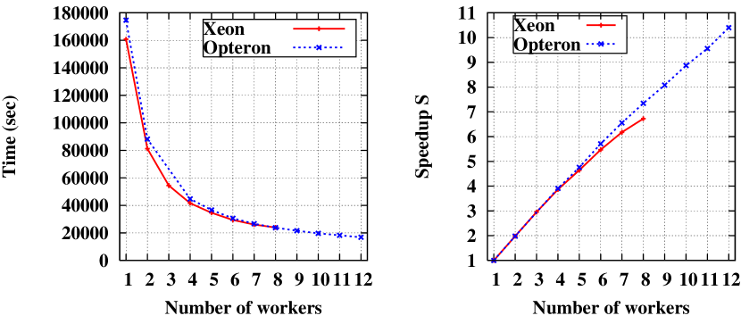
Figure 2: Absolute time and speedup for Xeon and Opteron computers.

As we can see, FIESTA scales on a Xeon computer essentially worse than on an Opteron one. Note that in both cases we have tested absolutely the same algorithm and software. The main hardware difference is a communication medium between processors and memory: Xeon has a shared Front-Side bus while Opteron uses point-to-point “hypertransport” mechanism.

Numerically the communication overhead can be very roughly estimated using the following formal model (see, e.g., [22]).

Let $\alpha$ be an essentially non-parallelizeable part of the job. The time spent by one worker is $T_{1}=\alpha T_{1}+(1-\alpha)T_{1}$, and $p$ workers time is $T_{p}=\alpha T_{1}+\frac{(1-\alpha)T_{1}}{p}+t_{d}$, where $t_{d}$ is the communication overhead. The speedup $S(p)=\frac{T_{1}}{T_{p}}=\frac{T_{1}}{\left(\frac{1-\alpha}{p}+\alpha\right)T_{1}+t_{d}}$, $t_{d}=0$ corresponds to the Amdahl’s law [23]: $S(p)=\left(\alpha+\frac{1-\alpha}{p}\right)^{-1}$.

Let us assume that the Opteron computer has a “good” communication medium, $t_{d}=\mbox{const}=b$, while the Xeon has a “bad” one, $t_{d}=b_{1}+b_{2}\times p$. We would like to fit numerically the Amdahl constant from the Opteron data and use it to estimate $b_{1}$ and $b_{2}$ for the Xeon data. If $t_{d}=\mbox{const}=b$ then it can be absorbed by the Amdahl constant $\alpha$. Indeed, let $\beta=\alpha+\frac{b}{T_{1}}$, then $S(p)=\frac{1}{\frac{1-\beta}{p}+\beta+\frac{b}{pT_{1}}}$. Assuming $b<<T_{1}$, the term $\frac{b}{pT_{1}}$ is negligible and will become zero by any good fit algorithm.

Fitting the Opteron data, we obtain $\alpha=0.0016$ (only 0.16 % is non-parallelizeable, including communication overhead) and then for the Xeon we get $b_{2}=428.305$ seconds per a CPU core, and $b_{1}$ is negligible. This means, running this FIESTA job with 8 CPU cores in parallel, the Xeon computer spends about 14 % of total time for communications.

The fitted speedup function for the Xeon computer has a maximum at 19 workers, and then it goes down. In Fig. 3 the fitted curve is extrapolated to the region beyond the theoretical maximum for this model which is only 9.54.

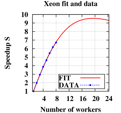
Figure 3: Data and extrapolated result for the Xeon fit.

FIESTA 1 is able to parallelize the C integration only on multicore computers. FIESTA 2 goes further, in the sense that one might set up a network of computers performing the integration. The communication is again performed via the Mathlink protocol since it can use not only the shared memory but also TCP/IP for data exchange.

One should not worry about the network traffic. Most of the time the processes work independently only exchanging keep-alive packets between each other. Moreover, the setup is relatively safe: if the network goes down, the main process keeps distributing tasks on a local machine and at the end recalculates the parts that were sent to remote machines and returned no answer. If a single integration process goes down it also does not spoil the calculation: FIESTA simply removes that particular process from the list of workers and resubmits its task elsewhere.

The tests show that moving, for example, from one 8-kernel machine to two 8-kernel machines gives more than a double speedup. The reason is that the main machine also works with a hard drive, while the other one is free from that.

To set up a calculation on multiple computers one has to launch slave tasks first. To do this one has to run CIntegrate -slave FILENAME on slave machines. (Usually one launches the number of slave processes equal to the number of kernels on the slave machine.) The FILENAME is the name of a file where the slave writes down some information about the IP-address of the slave machine and the two ports it is listening to. Unfortunately it is impossible to control the exact port number, therefore one might encounter problems if firewalls are turned on in the cluster. The file should be accessible from all the machines you wish to use in the parallel evaluation. Afterwards one can load FIESTA on the main machine, set RemoteLinksFile variable equal to the path to that file and launch the task.

4 Numerical instability

After the resolution of singularities, one often encounters functions like

$$\int_{0}^{1}\ldots\int_{0}^{1}\mbox{d}x_{i}\ldots\mbox{d}x_{n}\left(\prod_{j=1}^{n}x_{j}^{a_{j}-1+b_{j}\varepsilon}\right)Z,$$ (9)

where $Z$ has no singularities. Such a function still might have singularities because of non-positive $a_{j}$.

Let us assume that $a_{i}\leq 0$ and treat the integrand as a function $x^{a_{i}-1+b_{i}\varepsilon}Y(a_{i})$ with coefficients being polynomials in other variables. For readability we will omit the index $i$:

$$x^{a-1+b\varepsilon}Y(x)$$ (10)

To integrate such a function, the original FIESTA replaces (10) by

$$Y(0)x^{a-1+b\varepsilon}+Y^{\prime}(0)x^{a+b\varepsilon}+\ldots+\frac{1}{a!}Y^{(-a)}(0)x^{-1+b\varepsilon}+$$

$$x^{a-1+b\varepsilon}\left(Y(x)-Y(0)-Y^{\prime}(0)x-\ldots-\frac{1}{a!}Y^{(-a)}(0)x^{-a}\right)$$

The items in the first line of the expression can be integrated analytically over $x$ leaving us with one integration less. As for the remainder, it is known that it has no singularities at $x=0$ hence it can be expanded in $\varepsilon$ and integrated. However we result in integrating an expression that is a sum of potentially huge terms for small values of integration variables which sometime result in a nonsense when evaluated by a computer. As a workaround FIESTA 1 had the so-called IfCut’s — replacements of the integrand with its first terms of Taylor series for small values of integration variables. However, such an approach significantly slows the evaluation down and, more importantly, results in uncontrollable error estimates. Moreover, for some complicated situations problems start to appear even for really big values of integration variables, in pathological cases even setting the cut to $0.5$ (that is actually integrating something really different from the original function) makes this approach fail!

4.1 Resolving numerical instability by integration by parts

An alternative way to deal with expressions (10) is to use several times the integration by parts (IBP) formula in order to make the power of $x$ positive. However this method results in taking an extra derivative, and therefore all expressions become more complicated.

FIESTA 2 has an option ResolutionMode. The default value of this option is Taylor which reproduces the FIESTA 1 Taylor expansion. If one sets ResolutionMode to IBP0 then FIESTA 2 uses IBP with the representation $x^{a-1+b\varepsilon}=-\frac{\mbox{d}}{{\mbox{d}}x}\int_{x}^{1}t^{a-1+b\varepsilon}\mbox{d}t$. Since $\int_{1}^{1}t^{a-1+b\varepsilon}=0$, the surface term is equal to $Y(0)$. The third possibility for ResolutionMode is IBP1, in this case $x^{a-1+b\varepsilon}=\frac{\mbox{d}}{{\mbox{d}}x}\int_{0}^{x}t^{a-1+b\varepsilon}\mbox{d}t$ and the surface term is $Y(1)$.

Both of these resolution methods solve the problem of numerical instability but the efficiency might become very poor.

Let us consider the following simple example: the massless triangle with one zero external momentum so there is only one external momentum $p$, $p^{2}=-1$. Up to the constant part, the algorithm produces only six integrations. The most complicated integrand is the “number six” one. For ResolutionMode = IBP1 it looks like follows:

$$\frac{\log(1+x_{1})}{(1+x_{1})(2+x_{1})}-\frac{2\log(2+x_{1})}{(1+x_{1})(2+x_{1})}$$

$$+\frac{2}{(1+x_{2})(1+x_{1}+x_{2})^{2}}+\frac{\log(x_{1})}{(1+x_{2})(1+x_{1}+x_{2})^{2}}$$ (11)

$$+\frac{\log(1+x_{2})}{(1+x_{2})(1+x_{1}+x_{2})^{2}}-\frac{2\log(1+x_{1}+x_{2})}{(1+x_{2})(1+x_{1}+x_{2})^{2}}$$

and for ResolutionMode = Taylor it has the following form:

$$-\frac{\log(1+x_{1})}{(1+x_{1})^{2}}-\frac{1}{x_{1}(1+x_{2})^{2}}+\frac{1}{x_{1}(1+x_{2})(1+x_{1}+x_{2})}$$ (12)

At small $x_{1}$, the last two terms in (12) form a difference of two large numbers. Moreover, both these terms diverge at $x_{1}\to 0$ but their difference at $x_{1}=0$ is a smooth function. Indeed, contracting GCD (greatest common divisor) we obtain

$$-\frac{1}{x_{1}(1+x_{2})^{2}}+\frac{1}{x_{1}(1+x_{2})(1+x_{1}+x_{2})}=-\frac{1}{(1+x_{2})^{2}(1+x_{1}+x_{2})}.$$ (13)

Since there are only two integration variables, the function may be visualized as a 3D-plot, see Fig. 4.

Figure 4: 3D-plot of integrand obtained with ResolutionMode = Taylor, (12)

The function is very smooth and well suited for integration.

The function(11) has no non-integrable terms by construction. Nevertheless, it contains $\log(x_{1})$ and the shape of this function is much more complicated for integration, see Fig. 5.

Figure 5: 3D-plot of integrand obtained with ResolutionMode = IBP1, (11)

This is the common situation: the IBP methods produce much more terms, and an integrand behaves worse than that produced by the Taylor method. In fact, both IBP methods fail for complicated cases.

4.2 High-precision arithmetics

For technical reasons, one cannot make operations like (13) automatically. First of all, a GCD contraction is a very time-consuming operation. But more importantly, in a general case the Taylor approach results in expressions containing some logarithms after the $\varepsilon$ expansion, hence it is impossible to simplify the expression so that the large terms are canceled out. For example, some terms may contain factors like $\log(1+x)/x$.

Let us consider what happens during the integration more precisely.

For instance, let $x_{1}$ be $10^{-20}$. Then the last two terms in (12) are of order of $10^{20}$ but their difference is about $10^{-1}$. This means that all 20 leading decimal digits in fractions compensate each other and the result is obtained only from the difference in the fraction digits starting from 21. But in double precision IEEE arithmetics a fraction has only 14-15 reliable digits.

Provided that the fraction has 26 reliable decimal digits, the result contains 5 correct digits which is usually enough. So the natural idea appears, namely, to use ResolutionMode = Taylor together with a multiple precision floating-point arithmetics.

We have tested many different multiple precision floating-point libraries. The best one in our case appears to be the GNU mpfr library (http://www.mpfr.org).

One has to take into account that high-precision arithmetics libraries are much slower than the native hardware floating-point arithmetics, even for the same precision. Moreover, the larger precision is required, the slower calculations are. So there are two problems that arise:

1. Which points must be evaluated with the high-precision arithmetics and which ones might still remain in the native arithmetics?

2. Which precision must be set for the high-precision arithmetics?

In order to answer the first question let us try to find the worst case.

It is known by construction that all problems come from the negative powers of integration variables. Let us count maximal negative powers $max_{i}$ for each variable $x_{i}$ and construct the artificial auxiliary monomial

$$\prod_{i=1}^{n}x_{i}^{max_{i}}$$ (14)

where non-positive $max_{i}$ is the maximal negative power for $x_{i}$, or zero, if there are no negative powers for $x_{i}$. This monomial is the worst case in the sense that there are definitely no more dangerous terms.

Before evaluating the integrand at a concrete point $\vec{x}$ we calculate the monomial (14) at this point. If the result is larger than some threshold we might be in a trouble. In the native double precision IEEE arithmetics the fraction has 14-15 reliable decimal digits, so the default value for this threshold is $10^{9}$ in order to have 5-6 reliable decimal digits in the result. This value can be changed by means of the option MPThreshhold. If (14) at the point $\vec{x}$ is greater than the threshold value, the integrand at the point $\vec{x}$ is evaluated using the high-precision arithmetics.

Remember [13] that the C-part of FIESTA is an interpreter of a string representing an expression to be integrated. First, it compiles the integrand in some internal representation and then it integrates the function evaluating it many times. Precision for the high-precision arithmetics is fixed at the compile time after the monomial (14) is built. To do this, we again try to estimate the worst case.

We know that the function is smooth enough by construction, so a small shift in $\vec{x}$ should not change the result much.

Assume that the worst case would be when all $x_{i}$ are equal to some small value (0.001 by default, the user may change this value by the option SmallX). The exponent of (14) at this point roughly gives us the number of digits in the fraction we might lose.

Let $M$ be the value of (14) at SmallX. Since all numbers in a computer are of a binary format, the precision we need also is in bits (the IEEE double precision fraction has 53 bit). Calculating a binary logarithm of $M$ we get a number of bits in fractions we might lose, so then we have to add some bits for digits we would like to have in the fraction. The exact formula used by FIESTA in order to get the precision $p$ in bits is the following:

$$p=\log_{2}(M)+s$$ (15)

where $s$ is the number of reliable bits we would like to have in the fraction. The default value for $s$ is 38, it may be changed setting the option PrecisionShift.

Let us note that the user has the possibility to force FIESTA to use some fixed precision specifying the option DefaultPrecision, e.g. setting DefaultPrecision = 1024 forces the multiple precision to be 1024 independently on the result of evaluation (14) at SmallX.

As it was described above, the monomial (14) is calculated at each point $\vec{x}$ before evaluating the integrand. It might happen that the value of this monomial will be even more than $M$, which means the precision (15) might not be enough. In this case the algorithm increases all $x_{i}$ which are smaller than SmallX so that the value of (14) becomes not more than $M$. For this step, the user is able to specify the value which differs from $M$ by means of the option MPMin. The reason to have such an option is the following: for an expression like (10) we have essentially three different regions of our integration domain:

1. Native arithmetics.

2. High-precision arithmetics.

3. High-precision is not enough.

Sometimes it is useful to have the possibility to set the last region manually.

Let us summarize the high-precision arithmetics options here. Note that all these options are relevant only if the option ResolutionMode is set to Taylor.

• MPThreshhold is the value of (14) when the algorithm switches to high-precision arithmetics, default is $10^{9}$. This is essentially a big value so if the user specifies $\mbox{\tt MPThreshhold}<1$ then the algorithm uses the inverse value, $1/\mbox{\tt MPThreshhold}$. The bigger this value the better performance.

• SmallX is the value of $x$, $x_{1}=x_{2}=...=x_{n}=\mbox{\tt SmallX}$, where the value of (14) is evaluated in order to get the precision by the formula (15), default is 0.001. This is essentially a small value so if the user specifies $\mbox{\tt SmallX}>1$ then the algorithm uses the inverse value, $1/\mbox{\tt SmallX}$. The bigger this value the better performance.

• PrecisionShift is the number of reliable bits in intermediate calculation, the value of $s$ in (15), the default value is 38 which roughly corresponds to 11 decimal digits. The smaller this value the better performance.

• DefaultPrecision. If the user specifies this option then the algorithm uses this precision instead of (15). The minimal value for DefaultPrecision depends on the MPFR implementation, for mpfr-2.4.0 it is 2. The maximal value for DefaultPrecision is 2147483647. Setting DefaultPrecision=0 switches back to the default behaviour.

• MPMin. If the user specifies this option then the algorithm uses it instead of (14) at SmallX in order to check whether the high precision is enough or the current $\vec{x}$ should be cut of. This is essentially a big value so if the user specifies $\mbox{\tt MPMin}<1$ then the algorithm uses the inverse value, $1/\mbox{\tt MPMin}$. Setting $\mbox{\tt MPMin}<0$ switches back to the default behaviour. Changing this value does not influence the performance, the only reasons to set this option are debugging and profiling the code.

Note that all these options should be used with care. Playing with them, it is very easy to get a wrong result, e.g. increasing the value MPThreshhold the user may get better and better performance but suddenly the result might become completely wrong.

5 Speer sectors

As it has been explained in [24], Speer sectors can be also used as an iterative strategy for sector decompositions. However to use it one has to provide not only the propagators but also the diagram structure. Moreover, the Speer sectors are only applicable at all Euclidean external momenta. We have shown in that paper that in those cases our strategy S results in absolutely the same set of sectors. One might ask a reasonable question: why would one wish to use Speer sectors as a sector decomposition strategy at all? The answer is rather simple: since the Speer sectors strategy knows more information it can use it and work more efficiently, therefore performing the sector decomposition faster. For simple cases there is no reason to use them — one would spend more time providing the diagram structure correctly that one would win for the evaluation, but in some situations it might become crucial. Even more, the time and RAM required to make a sector decomposition step for strategy S grows exponentially with the complexity of the problem. In some cases the implementation of strategy S makes a failback to the non-efficient but straight-forward strategy A. Therefore in some complicated examples the implementation of strategy S might result in more sectors than an optimal strategy would produce, or, strategy S might even fail. To demonstrate this we provide examples of vacuum diagrams with equal masses on all lines, one vertex in the center and $N$ vertices around.

The following table compares the time and the number of sectors produced by strategies S and the Speer sectors strategy SS. Please, keep in mind that the diagrams have lots of internal symmetries, so actually only two primary sectors should be considered for each of those. To take this into consideration we used the PrimarySectorCoefficients option. For example, for the most complicated diagram, the hexagon, this option was set to {6,0,0,0,0,0,6,0,0,0,0,0} specifying that only the first and the seventh primary sectors should be considered and the results multiplied by $6$. The results are compared in the following table:

$N$	Strategy S - time	Strategy SS - time	Number of sectors
3	0.8	0.6	32
4	39	27	261
5	1859	1079	2574
6	F	40570	29450

At level $6$ the strategy $S$ could not produce a result because of memory overflow on a $2GB$ machine. (The sector decomposition stage does not use the hard drive and normally requires almost no RAM.)

Now let us provide instructions how to use strategy SS. As it has been said earlier, it is insufficient to set STRATEGY to STRATEGY_SS since the strategy has to use the information on the diagram. The evaluation is started not with

SDEvaluate[{U,F,l},indices,order],

but with

SDEvaluateG[graph_information,{U,F,l},indices,order].

The graph information should be of the form $\{lines,external\_vertices\}$, where $lines$ is a list of pairs of vertices connected by this line. The vertices should be numbered from $1$ without skipping numbers. It is also very important to have the order of lines coincide with the order of propagators in the $UF$ input. For example, for the hexagon the input is:

$$SDEvaluateG[\{\{\{1,2\},\{2,3\},\{3,4\},\{4,5\},\{5,6\},\{6,1\},$$

$$\{7,2\},\{7,3\},\{7,4\},\{7,5\},\{7,6\},\{7,1\}\},\{\}\},$$

$$UF[\{k1,k2,k3,k4,k5,k6\},$$

$$\{-k1^{2}+1,-k2^{2}+1,-k3^{2}+1,-k4^{2}+1,-k5^{2}+1,-k6^{2}+1,$$

$$-(k1-k2)^{2}+1,-(k2-k3)^{2}+1,-(k3-k4)^{2}+1,$$

$$-(k4-k5)^{2}+1,-(k5-k6)^{2}+1,-(k6-k1)^{2}+1\},\{\}],$$

$$\{1,1,1,1,1,1,1,1,1,1,1,1\},-1]$$

The diagram with all vertices numbered and all momenta labeled follows. The notation coincides with the notation of the input for FIESTA.

6 Additional features

6.1 Integrating at and above the threshold

Although the sector decomposition strategies are guaranteed to resolve singularities only if all terms of the function $F$ are of the same sign, FIESTA can sometimes succeed in a wider range of the problems. FIESTA tries to automatically find squares of differences of variables inside $F$ and to make special integration region decompositions before the sector decomposition. As a result, the code might succeed in evaluating Feynman integrals for (a) Feynman integrals at threshold. (b) Feynman integrals for the three-loop static potential. One of the examples recently calculated is the following:

This is a three-loop non-planar vertex at the threshold $(q_{1}+q_{2})^{2}=4M^{2}$. All solid lines are massive with mass $M$. The integrals of this type are used, for example, in heavy-fermion corrections to the three-loop matching coefficient of the vector current[32].

One might also try to produce the first poles of integrals above the threshold. To do that one must ensure that the UsingC option is set to False. Although one should use those results with care, we do not provide any guarantee for the correctness in this case.

6.2 Analytical results

Another reason to turn UsingC to False is to evaluate the highest poles analytically. In this case one should also set the ExactIntegrationOrder to the maximal $\varepsilon$ order that Mathematica should try to evaluate analytically and probably to change the timeout time ExactIntegrationTimeout for a single sector integral. The default value is $10$. After a timeout Mathematica proceeds with numerical evaluation.

Figure 6: The massless on-shell box diagram.

For example, for the box diagram (Fig. 6) with Mandelstam variables equal to $s=-3$ and $t=-1$ and UsingC=False the code normally returns

$$(1.333304\pm 0.000019)*\varepsilon^{-2}+(-0.732465\pm 0.000667)*\varepsilon^{-1}+(-4.386581\pm 0.000767)$$

If one sets ExactIntegrationOrder to 0, the result is

$$(4/3)*\varepsilon^{-2}+((-2*\log[3])/3)*\varepsilon^{-1}+(-4.386649\pm 0.00018)$$

Moreover, setting ExactIntegrationTimeout to 60 changes the result once more and we obtain

$$(4/3)*\varepsilon^{-2}+((-2*\log[3])/3)*\varepsilon^{-1}+((-4*Pi^{2})/9)$$

Of course, the minimal required timeout depends not only on the complexity of the problem but also on the CPU speed.

6.3 Different integrators

The original FIESTA used a Fortran implementation of Vegas as the integrator. Currently we have plugged in the Thomas Hahn Cuba library [29]. By default FIESTA uses the Vegas integrator, but this behavior can be easily controlled by the user, see the description of the option CurrentIntegrator in sect.8.

Cuba implements four algorithms for multidimensional numerical integration: Vegas, Suave, Divonne, and Cuhre. Cuhre is a deterministic algorithm, the others use Monte Carlo methods.

Vegas uses importance sampling for variance reduction. It is the simplest of the four but since the sector decomposition algorithm produces pretty good integrands the Vegas usually is the best choice.

Suave combines the advantages of two popular methods: importance sampling as done by Vegas and subregion sampling. Divonne works by stratied sampling, where the partitioning of the integration region is aided by methods from numerical optimization.

Cuhre is a deterministic algorithm, it uses a cubature rule for subregion estimation in a globally adaptive subdivision scheme. In low dimensions it may be used in hope to get the answer with high precision.

It is rather straightforward to add a new integrator to the C-code, see comments in the file “integrators.h”.

6.4 More general classes of integrals

The new version of FIESTA can be also applied to more general classes of integrals:

$$\int_{0}^{1}\ldots\int_{0}^{1}\mbox{d}x_{1}\ldots\mbox{d}x_{n}\prod_{j=1}\left[P_{j}\right]^{r_{j}}\;,$$ (16)

where $P_{j}$ are non-negative polynomials of $x_{i}$ and $r_{j}$ powers linearly dependent on a complex parameter $\varepsilon$.

The syntax is:

SDEvaluateDirect[x,P[1],P[2],…,P[n],r[1],r[2],…,r[n], order]

By default, FIESTA assumes that singularities in $\varepsilon$ arise only from regions of small values of integration variables $x[1],\ldots,x[n]$. However, one might specify the variables for which singularities in $\varepsilon$ are generated also at a vicinity of the value $x[i]=1$. The syntax is: BisectionVariables={i1,i2,i3,i4,i5} where $i1,\ldots$ correspond to such variables. To be on the safe side, one might list all the variables but this can decrease the performance essentially.

This new feature of FIESTA 2 was successfully applied to parametric integrals contributing to Wilson loops in [33] where it was used to check numerically analytic results.

7 Code installation

In order to install FIESTA 2, the user has to download the installation package
http://www-ttp.particle.uni-karlsruhe.de/$\sim$asmirnov/data/FIESTA_2.0.0.tar.gz,
unpack it and follow the instructions in the file INSTALL.

The Mathematica part of FIESTA requires almost no installation, one only needs to copy the FIESTA_2.0.0.m file and edit the default paths QLinkPath, CIntegratePath and DataPath in this file, for example:

• QLinkPath="/home/user/QLink/QLink";

• CIntegratePath="/home/user/FIESTA/CIntegrate";

• DataPath="/tmp/user/temp";

Here QLinkPath is a path to the executable QLink file, CIntegratePath is a path to the executable CIntegrate file, and DataPath is a path to the database directory. For the Windows system, these paths should look like

• QLinkPath="C:/programs/QLink/QLink.exe";

• CIntegratePath="C:/programs/FIESTA/CIntegrate.exe";

• DataPath="D:/temp";

Note that the program will create a big IO traffic to the directory DataPath, therefore, it is better to put this directory on a fast local disk.

Alternatively, one can specify all these paths manually after loading the file FIESTA_2.0.0.m into Mathematica.

Please note that the code requires Wolfram Mathematica 6.0 or 7.0 (recommended) to be installed and will not work correctly under lower versions of Mathematica.

In order to work with nontrivial integrals, the user must install QLink and the C-part of FIESTA, the CIntegrate program. The QLink [30] can be downloaded as a binary file or compiled from the sources. If the user decides to use pre-compiled CIntegrate executable file, he has to place the file to some location and edit the paths in the file FIESTA_2.0.0.m as it is described above. If the user wants to compile the executable file himself he must have several software packages to be installed on his computer.

First, the Mathematica Developer Kit. It should be installed if the user has the official Wolfram Mathematica installation.

The CIntegrate program depends on the MPFR library [31] and the Cuba library [29]. After installing MPFR and the Cuba library the user has to edit the self-explanatory Makefile and run the command “make”. Then, two executable files should appear, CIntegrate and CIntegrateMP. The first one uses the native IEEE floating-point arithmetic while CIntegrateMP uses the MPFR multi-precision library if necessary. CIntegrateMP is slightly slower than CIntegrate but it should produce a correct result for almost all integrals, so we strongly recommend to use CIntegrateMP

The C-sources are situated in the subdirectory “sources”. The program CIntegrate is compiled in the subdirectory “native” and the program CIntegrateMP is compiled in the subdirectory “mpfr”. After successful compilation both executable files are moved to the root FIESTA directory. In order to clean up the directory structure, the user may use the command “make clean”.

Under Windows the compilation should be performed under the Cygwin environment. In this case, the executable files will get the extension “.exe”.

8 Algorithm usage

To run FIESTA load the FIESTA_2.0.0.m into Wolfram Mathematica 6.0 or 7.0 To evaluate a Feynman integral one has to use the command

SDEvaluate[{U,F,l},indices,order],

where U and F are the functions defined by (2) and (3), l is the number of loops, indices is the set of indices and order is the required order of the $\varepsilon$-expansion.

There is a special syntax that is required to use the Speer sectors strategy, for details see section 5

To avoid manual construction of $U$ and $F$ one can use a build-in function UF and launch the evaluation as

SDEvaluate[UF[loop_momenta,propagators,subst],indices,order],

where subst is a set of substitutions for external momenta, masses and other values (note, the code performs numerical integrations. Thus the functions U and F should not depend on any external values).

To expand an integral by some variable tending to zero from the positive side, use the command

SDExpand[{U,F,l},indices,order,var,var order],

where var is the expansion variable and var order is the required variable expansion order. One should not care about the possible degrees of logarithms arising, they will be accounted automatically. Again it is possible to run the code with

SDExpand[UF[loop_momenta,propagators,subst],indices,order,var,var order]

Now the variable replacements should result in $U$ and $F$ depending only on var.

Examples:

SDEvaluate[UF[{k},{-k²,-(k+p₁)²,-(k+p₁+p₂)²,-(k+p₁+p₂+p₄)²},
{p${}_{1}^{2}\rightarrow$0,p${}_{2}^{2}\rightarrow$0,p${}_{4}^{2}\rightarrow$0, p₁ p${}_{2}\rightarrow$-s/2,p₂ p${}_{4}\rightarrow$-t/2,p₁ p${}_{4}\rightarrow$-(s+t)/2,
s$\rightarrow$-3,t$\rightarrow$-1}], {1,1,1,1},0]

performs the evaluation of the massless on-shell box diagram (Fig. 6) where the Mandelstam variables are equal to $s=-3$ and $t=-1$.

SDExpand[UF[{k},{-k²,-(k+p₁)²,-(k+p₁+p₂)²,-(k+p₁+p₂+p₄)²},
{p${}_{1}^{2}\rightarrow$0,p${}_{2}^{2}\rightarrow$0,p${}_{4}^{2}\rightarrow$0, p₁ p${}_{2}\rightarrow$-s/2,p₂ p${}_{4}\rightarrow$-t/2,p₁ p${}_{4}\rightarrow$-(s+t)/2,
s$\rightarrow$-1,t$\rightarrow$-tt}], {1,1,1,1},0,tt,0] expands the corresponding integral.

SDEvaluateDirect[x, P[1],P[2],... ,P[n], r[1],r[2],... ,r[n], order] evaluates the integral $\int_{0}^{1}\ldots\int_{0}^{1}\mbox{d}x_{1}\ldots\mbox{d}x_{n}\prod_{j=1}\left[P_{j}\right]^{r_{j}}\,.$

To clear the results from memory use the ClearResults[] command.

Here are the main options of the code (concerning high-precision arithmetics options see the end of the sect. 4.2). One should set the values before running the SDEvaluate command, e.g. NumberOfLinks=8):

• UsingC: specifies whether the C-integration should be used; default value: True;

• CIntegratePath: path to the CIntegrate binary;

• NumberOfLinks: number of the CIntegrate programs to be launched; default value: $1$;

• NumberOfSubkernels: number of Mathematica subkernels used; default value: $0$ (no Mathematica parallelization;

• UsingQLink: specifies whether QLink should be used to store data on disk; works only with UsingC=True; default value: True;

• QLinkPath: path to the QLink binary; we strictly recommend to use the new QLink binary working with the TokyoCabinet database and not with QDBM;

• DataPath: path to the place where QLink stores the data; for example, if DataPath=/temp/temp, then the code creates two files: /temp/temp1 and /temp/temp2; those files will be erased if existent; the directory /temp should exist;

Our recommendation for most complicated enough problems is to have UsingC and UsingQLink set to True; the NumberOfLinks and NumberOfSubkernels should be equal to the number of kernels on your computer; Mathematica 7.0 and the new version of QLink should be used. Also one should ensure that the DataPath directory does not point to a network drive.

There are other options that one can use:

• MixSectors: the number of sectors, that have to be integrated together. We do not recommend touching this option with UsingC=True, but if the Mathematica integration is on, one might set it to something big or even Infinity to optimize the integration speed;

• NegativeTermsHandling: the way the algorithm should deal with negative terms before the sector decomposition. Currently there are two options: "Squares" (default) and "None";

• CurrentIntegrator: the integrator used in C. Currently there are four options: "vegasCuba" (default option), "suaveCuba", "divonneCuba" and "cuhreCuba";

• CurrentIntegratorSetting: the options of the current integrator; run the job with default setting and you will see the current settings in the beginning of the output; they can copied to Mathematica and edited there. For details on those options see [29]];

• PrimarySectorCoefficients: The usage of this option allows to take the symmetries of the diagram into account. If the diagram has symmetries, then the primary sectors corresponding to symmetrical lines result in equal contributions to the integration result. Hence it makes sense to speed up the calculation by specifying the coefficients before the primary sector integrands. For example, if two lines in the diagram are symmetrical, one can have a zero coefficient before one of those and $2$ before the second. PrimarySectorCoefficients defines those coefficients if set; the size of this list should be equal to the number of primary sectors;

• STRATEGY: defines which sector decomposition strategy is used; STRATEGY_0 is not exactly a strategy, but an instruction not to perform the sector decomposition; STRATEGY_A and STRATEGY_B are the two strategies from Ref. [12] guaranteed to terminate; STRATEGY_S (default value) is our strategy, producing better results than the preceding ones; STRATEGY_SS is the strategy based on Speer sectors, one has to provide the diagram structure to use it; STRATEGY_X is an heuristic strategy from [12]; likely to share the ideas of Binoth and Heinrich [7]: powerful but not guaranteed to terminate; ResolutionMode: the method of dealing with singularities after the sector decomposition. Possible values: "IBP0", "IBP1" and "Taylor" (default value);

• RemoteLinksFile: the file where the code reads the information about remote slave CIntegrate jobs that can be used;

• RemoteLinksInstallTimeout: if a remote link cannot be installed after this amount of seconds, the code ignores the link;

• RemoteLinksTimeout: a timeout for reading a ready result from a remote link; after such a timeout the frozen link is banned for a minute for the first time and twice more each next time;

• ExactIntegrationOrder: the maximal order of $\varepsilon$ where FIESTA tries to present an analytical result; works only if UsingC is set to False.

• ExactIntegrationTimeout: the timeout for such an integration attempt for a single sector integral. The default value is $10$. After a timeout Mathematica proceeds with numerical evaluation.

• d0: the dimension of the space-time when $\varepsilon\rightarrow 0$; default value is $4$;

• ReturnErrorWithBrackets: if True, the code returns the error estimates in the form pm[57] and not pm57;

• BisectionVariables lists the variables for which the resolution of the singularities in $\varepsilon$ has to take into account a vicinity of the value $x[i]=1$. It is applied only with SDEvaluateDirect.

The following options are left for backward compatibility, but we recommend to avoid using them:

• IntegrationCut: the actual low boundary of the integration domain (instead of zero); default value: $0$;

• IfCut and VarExpansionDegree: if IfCut is nonzero then the expression is expanded up to order VarExpansionDegree over some of the integration variables; the integration function is evaluated exactly if the integration variable is greater that IfCut, otherwise the expansion is taken instead; the default value of IfCut is zero, the default value of VarExpansionDegree is $1$;

The following options were used in FIESTA 1 but have been completely removed from that moment:

• ForceMixingOfSectors: see MixSectors

• PrepareStringsWhileIntegrating: no analogue

• ResolveNegativeTerms: see NegativeTermsHandling

• VegasSettings: see CurrentIntegrator and CurrentIntegratorSettings

Some remarks on the usage of the code:

• In complicated cases one should use the QLink in order to store expressions on disk, otherwise there is a good chance to result in memory overflow;

• Wolfram Mathematica is sometimes very greedy in using RAM, to minimize this usage we minimize the internal Mathematica cache and keep erasing in constantly. If your jobs require this cache for optimization, then it is advised to run them in a separate Mathematica session

• The package compilation results in two CIntegrate binary files — with the multiprecision and without it. Although the multiprecision binary is slower, it is advised to use it to avoid the numerical instability problems (even if you are aiming at a few digits for your integral, the high precision arithmetics is required in between, see section 4.2).

• For complicated integrals it makes sense to increase the number of integral evaluations performed during the integration (otherwise the algorithm might fail to adapt to all peaks and underestimate the error). The default value is $50000$, while the FIESTA 1 default value was $1500000$. Such a small number leads to very fast integration but the obtained value of the integral is usually only a rough estimation which is nevertheless enough to check numerically the correctness of the known analytical result. This setting can be adjusted by the option CurrentIntegratorSettings. To get a real answer with several reliable digits one should set something like ${\tt CurrentIntegratorSettings}=$

  $\{\{"maxeval","1500000"\},\{"nincrease","10000"\}$.

9 Numerical results

In [25] a set of the four-loop massless propagator master integrals was identified. Analytical results in expansion in $\varepsilon$ for these integrals will be published soon [26]. Using FIESTA we have calculated the most complicated integrals of this family and obtained a good agrement with the analytical results. Here we consider one of the most complicated diagrams which is shown in Fig. 1. As usually, it is implied within FIESTA that Feynman integrals are with the $-k^{2}-i0$ dependence of propagators and results are presented, in a Laurent expansion in $\varepsilon$, by pulling out the factor $i\pi^{d/2}e^{-\gamma_{E}\varepsilon}$ per loop, where $\gamma_{E}$ is the Euler constant.

Degree	Exact	Cuba Vegas	Cuba Vegas
of $\varepsilon$:	Value:	500 000 result:	1 500 000 result:
$\varepsilon^{-1}$	-10.3692776	-10.36941 $\pm$ 0.00011	-10.36931 $\pm$ 0.00006
$\varepsilon^{0}$	-70.99081719	-70.989 $\pm$ 0.002	-70.990 $\pm$ 0.0011
$\varepsilon^{1}$	-21.663005	-21.633 $\pm$ 0.023	-21.650 $\pm$ 0.013
$\varepsilon^{2}$	—	2832.86 $\pm$ 0.17	2832.69 $\pm$ 0.096()

Table 1: Numerical results for one of the most complicated four-loop propagator master integrals. In the second column, the numerical values of the known analytical results are shown. The last two columns contain the results of evaluation of these integrals by FIESTA using the Cuba VEGAS integrator with 500000 and 1500000 sampling points. The integral is calculated up to one extra power of $\varepsilon$ which is unknown analytically.

Degree	Cuba Vegas		Cuba Vegas
of $\varepsilon$:	500 000 time:		1 500 000 time:
$\varepsilon^{-1}$	2262.	86s	3495.	28s
$\varepsilon^{0}$	15242.	10s	39673.	48s
$\varepsilon^{1}$	61481.	36s	162453.	52s
$\varepsilon^{2}$	202018.	31s	1794640.	00s()
Total time:	768727.	00s	—

Table 2: Timing for calculations of the most complicated master integral. The last two columns contain times (in seconds) of numerical integration by the Cuba VEGAS integrator with 500000 and 1500000 sampling points. Also a total time for evaluation of the integral is given, including the Mathematica part.

We use the Cuba VEGAS integrator with different parameters for the numerical integration. Comparing with the analytical results (Table 1), the restriction in 500 000 sampling points leads to the numerical result with 3-4 reliable digits in a quite reasonable time (see Table 2) while the integration with 1 500 000 sampling points reproduces the analytical results with 4-5 digits. We also have evaluated one extra $\varepsilon$ term expansion which is unavailable analytically. For some technical reasons, for the highest $\varepsilon$ term of the integral with 1 500 000 sampling points, we have restricted ourselves with the value produced by the FORTRAN VEGAS integrator which is not supported anymore.

10 Conclusion

We have presented an essentially updated version of our algorithm. It can be now used not only for evaluating Feynman integrals by sector decomposition but also for expanding Feynman integrals in various limits of momenta and masses. We have demonstrated the new features with examples. We believe FIESTA 2 to be an important tool for practical calculations and cross-checks of analytical results.

Acknowledgments. We are grateful to K.G. Chetyrkin for useful discussions and to P. Marquard and M. Steinhauser for testing our code on numerous examples. This work was supported in part by DFG through SBF/TR 9 and the Russian Foundation for Basic Research through grant 08-02-01451.

References

- [1] K. Hepp, Commun. Math. Phys. 2 (1966) 301.
-
[2]
E. R. Speer,
J. Math. Phys., 9 (1968) 1404;
M. C. Bergère and J. B. Zuber, Commun. Math. Phys. 35 (1974) 113;
M. C. Bergère and Y. M. Lam, J. Math. Phys. 17 (1976) 1546;
O. I. Zavialov, Renormalized quantum field theory, Kluwer Academic Publishers, Dodrecht (1990);
V. A. Smirnov, Commun. Math. Phys. 134 (1990) 109. -
[3]
P. Breitenlohner and D. Maison,
Commun. Math. Phys. 52 (1977) 11; 39,55;
-
[4]
M. C. Bergère, C. de Calan and A. P. C. Malbouisson,
Commun. Math. Phys. 62 (1978) 137;
K. Pohlmeyer, J. Math. Phys. 23 (1982) 2511. - [5] V. A. Smirnov, Applied asymptotic expansions in momenta and masses, STMP 177, Springer, Berlin, Heidelberg (2002).
- [6] E. R. Speer, Ann. Inst. H. Poincaré, 23 (1977) 1.
- [7] T. Binoth and G. Heinrich, Nucl. Phys. B, 585 (2000) 741; Nucl. Phys. B, 680 (2004) 375; Nucl. Phys. B, 693 (2004) 134.
- [8] G. Heinrich, Int. J. of Modern Phys. A, 23 (2008) 10. [arXiv:0803.4177].
- [9] V. A. Smirnov, Phys. Lett. B 567 (2003) 193 [arXiv:hep-ph/0305142].
-
[10]
T. Gehrmann, G. Heinrich, T. Huber and C. Studerus,
Phys. Lett. B 640 (2006) 252
[arXiv:hep-ph/0607185];
G. Heinrich, T. Huber and D. Maitre, Phys. Lett. B 662 (2008) 344 [arXiv:0711.3590 [hep-ph]]. - [11] R. Boughezal and M. Czakon, Nucl. Phys. B 755 (2006) 221 [arXiv:hep-ph/0606232].
- [12] C. Bogner and S. Weinzierl, Comput. Phys. Commun. 178 (2008) 596 [arXiv:0709.4092 [hep-ph]]; Nucl. Phys. Proc. Suppl. 183 (2008) 256 [arXiv:0806.4307 [hep-ph]].
- [13] A. V. Smirnov and M. N. Tentyukov, Comput. Phys. Commun. 180 (2009) 735 [arXiv:0807.4129 [hep-ph]].
-
[14]
A. V. Smirnov, V. A. Smirnov and M. Steinhauser,
Phys. Lett. B 668, 293 (2008)
[arXiv:0809.1927 [hep-ph]];
R. Bonciani and A. Ferroglia, JHEP 0811, 065 (2008) [arXiv:0809.4687 [hep-ph]];
Y. Kiyo, D. Seidel and M. Steinhauser, JHEP 0901, 038 (2009) [arXiv:0810.1597 [hep-ph]];
G. Bell, Nucl. Phys. B 812, 264 (2009) [arXiv:0810.5695 [hep-ph]];
V. N. Velizhanin, arXiv:0811.0607 [hep-th];
T. Ueda and J. Fujimoto, arXiv:0902.2656 [hep-ph];
D. Seidel, arXiv:0902.3267 [hep-ph];;
G. Heinrich, T. Huber, D. A. Kosower and V. A. Smirnov, Phys. Lett. B 678, 359 (2009) [arXiv:0902.3512 [hep-ph]];
P. A. Baikov, K. G. Chetyrkin, A. V. Smirnov, V. A. Smirnov and M. Steinhauser, Phys. Rev. Lett. 102, 212002 (2009) [arXiv:0902.3519 [hep-ph]];
J. Gluza, K. Kajda, T. Riemann and V. Yundin, PoS A CAT08, 124 (2008) [arXiv:0902.4830 [hep-ph]];
S. Bekavac, A. G. Grozin, D. Seidel and V. A. Smirnov, Nucl. Phys. B 819, 183 (2009) [arXiv:0903.4760 [hep-ph]];
R. Bonciani, A. Ferroglia, T. Gehrmann and C. Studerus, JHEP 0908, 067 (2009) [arXiv:0906.3671 [hep-ph]];
M. Czakon, A. Mitov and G. Sterman, Phys. Rev. D 80, 074017 (2009) [arXiv:0907.1790 [hep-ph]];
A. Ferroglia, M. Neubert, B. D. Pecjak and L. L. Yang, arXiv:0907.4791 [hep-ph]; JHEP 0911, 062 (2009) [arXiv:0908.3676 [hep-ph]];
S. Bekavac, A. G. Grozin, P. Marquard, J. H. Piclum, D. Seidel and M. Steinhauser, arXiv:0911.3356 [hep-ph];
M. Dowling, J. Mondejar, J. H. Piclum and A. Czarnecki, arXiv:0911.4078 [hep-ph];
A. V. Smirnov, V. A. Smirnov and M. Steinhauser, [arXiv:0911.4742 [hep-ph]]. -
[15]
M. Beneke and V. A. Smirnov,
Nucl. Phys. B 522, 321 (1998);
V. A. Smirnov and E. R. Rakhmetov, Theor. Math. Phys. 120, 870 (1999) [Teor. Mat. Fiz. 120, 64 (1999)];
V. A. Smirnov, Phys. Lett. B 465, 226 (1999). - [16] V. Pilipp, JHEP 0809 (2008) 135.
-
[17]
V. A. Smirnov, Phys. Lett. B 460 (1999) 397;
J. B. Tausk, Phys. Lett. B 469 (1999) 225;
M. Czakon, Comput. Phys. Commun. 175 (2006) 559;
A. V. Smirnov and V. A. Smirnov, arXiv:0901.0386 [hep-ph]. -
[18]
V. A. Smirnov, Evaluating Feynman Integrals, Springer Tracts
Mod. Phys. 211 (2004) 1;
V. A. Smirnov, Feynman integral calculus, Berlin, Germany: Springer (2006) 283 p. -
[19]
M. Roth and A. Denner, High-energy approximation of one-loop Feynman
integrals, Nucl. Phys. B479 (1996) 495–514,
[hep-ph/9605420];
A. Denner, M. Melles and S. Pozzorini, Nucl. Phys. B 662 (2003) 299 [hep-ph/0301241];
S. Pozzorini, Nucl. Phys. B 692, 135 (2004) [hep-ph/0401087];
A. Denner and S. Pozzorini, Nucl. Phys. B 717 (2005) 48 [arXiv:hep-ph/0408068];
A. Denner, B. Jantzen and S. Pozzorini, Nucl. Phys. B 761 (2007) 1 [arXiv:hep-ph/0608326]; arXiv:0801.2647 [hep-ph]; JHEP 0811 (2008) 062 [arXiv:0809.0800 [hep-ph]]; -
[20]
C. Anastasiou, K. Melnikov and F. Petriello,
Phys. Rev. D 69 (2004) 076010
[arXiv:hep-ph/0311311];
Phys. Rev. Lett. 93 (2004) 032002
[arXiv:hep-ph/0402280];
Phys. Rev. Lett. 93 (2004) 262002
[arXiv:hep-ph/0409088];
Nucl. Phys. B 724 (2005) 197
[arXiv:hep-ph/0501130];
JHEP 0709 (2007) 014
[arXiv:hep-ph/0505069];
G. Heinrich, Nucl. Phys. Proc. Suppl. 157 (2006) 43 [arXiv:hep-ph/0601232]; Eur. Phys. J. C 48 (2006) 25 [arXiv:hep-ph/0601062]. - [21] T. Kaneko and T. Ueda, arXiv:0908.2897 [hep-ph].
- [22] M. Horoi and R. J. Enbody, International Journal of High Performance Computing Applications, 15, No. 1, 75–80 (2001).
- [23] G. M. Amdahl, Validity of the Single Processor Approach to Achieving Large-Scale Computing Capabilitie, In: Proc. AFIPS Conf., 1967, Reston, VA, USA.
- [24] A. V. Smirnov and V. A. Smirnov, JHEP, 05 (2009) 004 [arXiv:0812.4700 [hep-ph]].
- [25] P. A. Baikov, Phys. Lett. B 634, 325 (2006) [arXiv:hep-ph/0507053].
- [26] P. A. Baikov and K. G. Chetyrkin, in preparation.
- [27] G. ’t Hooft and M. Veltman, Nucl. Phys. B44 (1972) 189.
- [28] C. G. Bollini and J. J. Giambiagi, Nuovo Cim. 12B (1972) 20.
- [29] T. Hahn, Comput. Phys. Commun. 168 (2005) 78 [arXiv: hep-ph/0404043].
- [30] QLink – open-source program by A.V. Smirnov, http://qlink08.sourceforge.net
- [31] GNU MPFR http://www.mpfr.org/ is a portable C library for arbitrary-precision binary floating-point computation with correct rounding, based on GMP library http://gmplib.org/
- [32] P. Marquard, J. H. Piclum, D. Seidel and M. Steinhauser, Phys. Lett. B 678, 269 (2009) [arXiv:0904.0920 [hep-ph]].
- [33] V. Del Duca, C. Duhr and V. A. Smirnov, arXiv:0911.5332 [hep-ph].