June 2016
TTK-16-19 The perturbative QCD gradient flow
to three loops

Abstract

The gradient flow in QCD is treated perturbatively through next-to-next-to-leading order in the strong coupling constant. The evaluation of the relevant momentum and flow-time integrals is described, including various means of validation. For the vacuum expectation value of the action density, which turns out to be a useful quantity in lattice calculations, we find a very well-behaved perturbative series through NNLO. Quark mass effects are taken into account through NLO. The theoretical uncertainty due to renormalization-scale variation is significantly reduced with respect to LO and NLO, as long as the flow time is smaller than about 0.1 fm.

1 Introduction

QCD is a remarkable theory in many respects. It has been unchallenged in the description of strong interactions since its original formulation of more than 40 years ago [1]. It crucially impacts theoretical descriptions of a vast range of observations, reaching from the hadron mass spectrum to cross sections at particle colliders. When quarks are neglected (quenched QCD), the only fundamental parameter of QCD is the strong coupling constant $\alpha_{s}$, which simultaneously defines a mass scale $\Lambda_{\text{{QCD}}}\sim{\cal O}(100\,\text{MeV})$ due to its momentum dependence implied by quantum field theory (dimensional transmutation). Also, due to asymptotic freedom[2, 3], QCD does not have an ultra-violet cut-off; it remains consistent up to arbitrarily high energies.

A very successful approach for calculations based on the QCD Lagrangian is perturbation theory. It corresponds to an expansion in the strong coupling constant $\alpha_{s}$ and is applicable for processes where the typical mass scale $Q$ is much larger than $\Lambda_{\text{{QCD}}}$. The natural input quantity is therefore $\alpha_{s}$, whose numerical value at a reference scale $Q_{0}\gg\Lambda_{\text{{QCD}}}$ is determined by comparing theoretical predictions with measurements for known processes. Any dependence of physical observables on $\Lambda_{\text{{QCD}}}$ is only implicit through $\alpha_{s}$:

$$\begin{split}\alpha_{s}(Q)\simeq\frac{1}{\beta_{0}\log(Q^{2}/\Lambda_{\text{{QCD}}}^{2})}\,,\end{split}$$ (1)

where $\beta_{0}$ is the leading order coefficient of the QCD $\beta$ function and will be defined below.

Perturbation theory is obviously inadequate for calculating observables like the hadron mass spectrum or the pion decay constant which are strongly dependent on $\Lambda_{\text{{QCD}}}$. Such problems are accessible in lattice gauge theory, however[4]. In this approach, space-time is discretized by a characteristic lattice spacing $a$ which serves as a UV regulator.

Unfortunately, lattice gauge theory and perturbation theory are not only complementary approaches to QCD, but there is practically no overlap region where both would yield competitive results. There is a certain amount of cross-fertilization though, in particular in the context of renormalization [5, Chetyrkin:1999pq, Capitani:1998mq, Dolgov:2002zm] or flavor physics (for a review, see Ref.[Colangelo:2010et], for example).

A particularly promising theoretical quantity which is accessible both perturbatively and on the lattice is the so-called Yang-Mills gradient flow [Narayanan:2006rf, Luscher:2009eq, Luscher:2010iy, Luscher:2011bx]. For a particular gauge invariant quantity (the so-called QCD action density, to be defined in more detail below), it was shown by Lüscher [Luscher:2010iy] that it exhibits some welcome features on the lattice which allows its efficient evaluation with rather high precision. He also explicitly calculated this quantity perturbatively through next-to-leading order (NLO) and showed that the standard QCD renormalization of the gauge coupling constant is sufficient in order to obtain a finite result[Luscher:2010iy]. This property was later proven to all orders in perturbation theory[Luscher:2011bx]. The perturbative and the lattice result were found to be compatible over a significant interval of the so-called flow-time parameter $t$, thus opening up a wide range of possibilities for cross-fertilization in both fields.

In lattice QCD, the benefits and the appeal of the gradient flow have already been established, for example in its use for determining the absolute mass scale of a lattice calculation[Luscher:2010iy, Borsanyi:2012zs] (“scale setting”, see Ref.[Sommer:2014mea], for example). From the perturbative point of view, on the other hand, the concept has received almost no attention since the original works of Refs.[Luscher:2010iy, Luscher:2011bx]. However, since one may expect rather precise results on the lattice in this framework, this may pose a challenge for perturbative calculations as well, possibly leading to interesting first-principle results for QCD.

With this motivation in mind, we are going to study the QCD action density in the framework of the gradient flow up to next-to-NLO (NNLO) in a perturbative approach. The perturbative expansion will be obtained via Wick contractions of the original field operators. This results in three $D$-dimensional momentum and up to four flow-time integrations over products of massless Feynman propagators times exponential factors involving loop momenta and flow-time integration variables. They are solved by sector decomposition and suitable numerical integration routines. While quark-mass effects will be neglected in the NNLO calculation, we show that they can be included through a simple one-dimensional integral at NLO.

The remainder of this paper is organized as follows. In the next section, after briefly recalling the flow-field formalism, the generation of the perturbative series and the evaluation of the resulting integrals is described. Additionally, we give a list of checks performed on our calculation, validating the numerical as well as the conceptional steps. In Section 3, we present the numerical value for the NNLO coefficient of the action density, which is the main result of this paper, and provide a brief analysis of the numerical effects. We conclude and give a short outlook on possible extensions and applications of this work in Section 4.

2 Formalism

2.1 The flow field

The theoretical framework of our calculation is defined by the equations [Luscher:2011bx, Luscher:2010iy]

$$\begin{split}\partial_{t}B^{a}_{\mu}&=D^{ab}_{\nu}G^{b}_{\nu\mu}+(1-\lambda)\,D^{ab}_{\mu}\partial_{\nu}B^{b}_{\nu}\,,\qquad B^{a}_{\mu}(t=0,x)=g_{0}A^{a}_{\mu}(x)\,,\\ G^{a}_{\mu\nu}&=\partial_{\mu}B^{a}_{\nu}-\partial_{\nu}B^{a}_{\mu}+if^{abc}B^{b}_{\mu}B^{c}_{\nu}\,,\qquad D^{ab}_{\mu}=\delta^{ab}\partial_{\mu}-if^{abc}B^{c}_{\mu}\,,\end{split}$$ (2)

where $B^{a}_{\mu}(t,x)$ is the flow field with space-time index $\mu$ and color index $a$, $g_{0}$ is the bare QCD coupling constant, $f^{abc}$ are the SU(3) structure constants, and $A^{a}_{\mu}(x)$ is the fundamental gauge field of QCD. The derivative $\partial_{\mu}$ is understood w.r.t. the $D$-dimensional Euclidean space-time variable $x$, while $t$ denotes the so-called flow-time. It is easily seen [Luscher:2010iy] that solutions of Eq. (2) for different values of $\lambda$ are related by a $t$-dependent gauge transformation of the flow field $B_{\mu}$.

It was shown in Ref.[Luscher:2011bx] that the flow equation (2) can be written as the following integral equation in momentum space:

$$\begin{split}\tilde{B}_{\mu}^{a}(t,p)\equiv\int\text{d}^{D}x\,e^{-ipx}B^{a}_{\mu}(t,x)=g_{0}\,\tilde{K}_{\mu\nu}(t,p)\tilde{A}^{a}_{\nu}(p)+\int_{0}^{t}\text{d}s\,\tilde{K}_{\mu\nu}(t-s,p)\tilde{R}^{a}_{\nu}(s,p)\,,\end{split}$$ (3)

where

$$\begin{split}\tilde{K}_{\mu\nu}(t,z)=e^{-tp^{2}}\delta_{\mu\nu}-\frac{p_{\mu}p_{\nu}}{p^{2}}e^{-tp^{2}}\left(1-e^{\lambda tp^{2}}\right)\,,\end{split}$$ (4)

and

$$\tilde{R}_{\mu}^{a}(t,p)=\sum_{n=2}^{3}\frac{1}{n!}\int_{q_{1}}\cdots\int_{q_{n}}(2\pi)^{D}\delta(p+q_{1}+\cdots+q_{n})\\ \times X^{(n,0)}(q_{1},\ldots,q_{n})^{ab_{1}\cdots b_{n}}_{\mu\nu_{1}\cdots\nu_{n}}\tilde{B}_{\nu_{1}}^{b_{1}}(t,-q_{1})\cdots\tilde{B}_{\nu_{n}}^{b_{n}}(t,-q_{n})\,,$$ (5)

with $\int_{p}\equiv\int\frac{\mathrm{d}^{D}p}{(2\pi)^{D}}$. The vertices $X^{(n,0)}$ read

$$\begin{split}X^{(2,0)}(q,r)^{abc}_{\mu\nu\rho}=&\ if^{abc}\big{\{}(r-q)_{\mu}\delta_{\nu\rho}+2q_{\rho}\delta_{\mu\nu}-2r_{\nu}\delta_{\mu\rho}-\lambda(q_{\nu}\delta_{\mu\rho}-r_{\rho}\delta_{\mu\nu})\big{\}}\,,\\ X^{(3,0)}(q,r,s)_{\mu\nu\rho\sigma}^{abcd}=&\ f^{abe}f^{cde}(\delta_{\mu\sigma}\delta_{\nu\rho}-\delta_{\mu\rho}\delta_{\sigma\nu})\\ &+f^{ade}f^{bce}(\delta_{\mu\rho}\delta_{\nu\sigma}-\delta_{\mu\nu}\delta_{\rho\sigma})+f^{ace}f^{dbe}(\delta_{\mu\nu}\delta_{\rho\sigma}-\delta_{\mu\sigma}\delta_{\nu\rho})\,.\end{split}$$ (6)

The fact that the first term in Eq. (3) is proportional to $g_{0}$ allows an iterative solution of that equation, which leads to an asymptotic series for $B_{\mu}^{a}$,

$$\begin{split}B_{\mu}^{a}=\sum_{n\geq 1}g_{0}^{n}B_{n,\mu}^{a}\,.\end{split}$$ (7)

With each power of $g_{0}$, the number of fundamental gauge fields $A_{\mu}^{a}$ increases by one. Furthermore, $B_{n,\mu}^{a}$ involves terms with $\lceil n/2\rceil,\lceil n/2\rceil+1,\ldots,n-1$ flow-time integrations, where $\lceil n/2\rceil$ denotes the greatest integer less than or equal to $n/2$.

Note that Eqs. (4) and (6) become particularly simple for $\lambda=0$; for example, the lowest-order solution of the flow-field equation is simply $\tilde{B}_{\mu}^{a}(t,p)=e^{-tp^{2}}\tilde{A}_{\mu}^{a}(p)$ in this case.

2.2 Calculation of the action density

The quantity to be computed in this paper is the vacuum expectation value of the action density,

$$\begin{split}E(t,x)\equiv\frac{1}{4}\,G^{a}_{\mu\nu}G^{a}_{\mu\nu}\,.\end{split}$$ (8)

Since $E(t,x)$ is gauge invariant, we are allowed to set $\lambda=0$ in our calculation, which minimizes the number of integrals to be evaluated. The case $\lambda\neq 0$ will be considered as an important check of our calculation in Sect. 2.4.

The perturbative expansion of the vacuum expectation value

$$\begin{split}\langle E\rangle=\frac{1}{2}\langle\partial_{\mu}B_{\nu}^{a}\partial_{\mu}B_{\nu}^{a}-\partial_{\nu}B_{\mu}^{a}\partial_{\nu}B_{\mu}^{a}\rangle+f^{abc}\langle(\partial_{\mu}B_{\nu}^{a})B_{\mu}^{b}B_{\nu}^{c}\rangle+\frac{1}{4}f^{abc}f^{cde}\langle B_{\mu}^{a}B_{\nu}^{b}B_{\mu}^{c}B_{\nu}^{d}\rangle\end{split}$$ (9)

is obtained by inserting the asymptotic expansion of the flow field $B_{\mu}^{a}$ as obtained in the previous section, and including higher orders of the fundamental perturbative vacuum, i.e.

$$\begin{split}\langle{\cal O}\rangle=\frac{\langle 0|{\cal O}\exp(-S_{\text{{QCD}}}(g_{0}))|0\rangle}{\langle 0|\exp(-S_{\text{{QCD}}}(g_{0}))|0\rangle}\,,\end{split}$$ (10)

where $S_{\text{{QCD}}}$ is the interaction part of the fundamental QCD action which depends on the fundamental gauge fields $A_{\mu}^{a}$.

From Eqs. (9) and (3) it follows that $\langle E\rangle={\cal O}(g_{0}^{2})$; only the first term on the r.h.s. of Eq. (9) contributes at lowest order, while the second and the third term are of order $g_{0}^{4}$ (odd powers in $g_{0}$ vanish due to an odd number of fields in the matrix elements). However, all three terms on the r.h.s. of Eq. (9) contribute to higher orders as well, either through higher orders in the expansion of the $B$-fields, see Eq. (3), or through the perturbative expansion of the exponential in Eq. (10). The former case generally leads to an increase in the number of flow-time integrations, while the latter corresponds to corrections due to fundamental QCD. The general form of a matrix element to be evaluated at order $g_{0}^{n}$ can therefore be symbolized by

$$\begin{split}M_{n}(k,m)\equiv\langle 0|(B_{m_{1}}\cdots B_{m_{k}})\times\left(S_{\text{{QCD}}}\right)^{n-m}|0\rangle\,,\qquad m=\sum_{i=1}^{k}m_{i}\,,\end{split}$$ (11)

where $B_{m_{i}}$ is the $m_{i}^{\text{th}}$ coefficient of the asymptotic series in Eq. (7). This classification turns out useful with respect to the way we subsequently simplify the matrix elements in the sense that individual terms cannot be combined among different classes. Note that $0\leq m-k$ is the maximum number of flow-time integrations in $M_{n}(k,m)$, and since $m\leq n$, the maximum number of flow-time integrations at order $g_{0}^{n}$ is $n-2$.

One particularly simple class when calculating $\langle E\rangle$ is $M_{n}(2,2)$, which is fully determined by the $(n-2)$-loop self-energy of the fundamental gluon field; this will serve as a welcome check of our calculation, see Sect. 2.4. At LO, $M_{2}(2,2)$ is in fact the only class that contributes. At order $g_{0}^{n}$ for $n\geq 4$, one needs to evaluate $3(n-2)$ classes, namely $M_{n}(k,m)$ with $k\in\{2,3,4\}$ and $k\leq m\leq n$. Thus, at NNLO, there are twelve classes that contribute to $\langle E\rangle$, and the maximum number of flow-time integrations is four. For comparison, at NLO there are six classes and at most two flow-time integrations.

2.3 Evaluation of the perturbative series

Except for the final numerical integration, all stages of the calculation were performed with the help of Mathematica[mathematica70]. Rather than following the diagrammatic method developed in Ref.[Luscher:2011bx], we directly implemented the Wick contractions of the gauge and quark fields after the iterative expansion of the flow fields according to Eqs. (3) and (5), the perturbative expansion of $\exp(-S_{\text{{QCD}}})$ in Eq. (10), and the insertion of QCD-Feynman rules. The Dirac algebra is performed with the functionalities of FeynCalc[Mertig:1990an] and color factors are calculated using ColorMath[Sjodahl:2012nk]; vacuum diagrams are discarded as required by the normalization factor in Eq. (10).

After these algebraic and symbolic manipulations, one ends up with integrals of the general form (at ${\cal O}(g_{0}^{6})$)

$$\begin{split}&I(t,{\bf n},{\bf a},D)=\left(\prod_{f=1}^{N}\int_{0}^{t_{f}^{\text{up}}}\text{d}t_{f}\right)\int_{p_{1},p_{2},p_{3}}\frac{\exp[\sum_{k,i,j}a_{kij}t_{k}p_{i}p_{j}]}{p_{1}^{2n_{1}}p_{2}^{2n_{2}}p_{3}^{2n_{3}}p_{4}^{2n_{4}}p_{5}^{2n_{5}}p_{6}^{2n_{6}}}\,,\end{split}$$ (12)

where $D=4-2\epsilon$ is the space-time dimension,

$$\begin{split}{\bf n}&=\{n_{1},n_{2},n_{3},n_{4},n_{5},n_{6}\}\,,\\ {\bf a}&=\{a_{kij}:k=0,\ldots,N\,;\,i=1,2,3\,;j=1,2,3\}\end{split}$$ (13)

are sets of integers, $N\leq 4$, $t_{0}\equiv t$, and the upper limits for the flow-time integrations are linear combinations of the other flow-time variables, $t_{f}^{\text{up}}=t_{f}^{\text{up}}(t_{0},\ldots t_{f-1})$. The momenta $p_{4}$, $p_{5}$, $p_{6}$ are linear combinations of the integration momenta $p_{1}$, $p_{2}$, $p_{3}$. Quark-mass effects have been neglected in Eq. (12); at NLO, we will take them into account in Sect. 2.5.

Needless to say that in order to minimize computer time, it is important to identify integrals which differ by linear transformations of the loop momenta and flow-time integration variables at this stage, to cancel numerators with denominators in the integrals as far as possible, and to discard scale-less integrals which vanish in dimensional regularization. After these simplifications, the number of integrals of the form given in Eq. (12) is listed in Table 1, both split according to the classification defined in Eq. (11), and according to the number of flow-time integrations. For comparison, we also give the corresponding numbers for the NLO case in Table 2.

$k$ 2 3 4 $\Sigma$ $m$ 2 3 4 5 6 3 4 5 6 4 5 6 # 24 45 219 683 2244 13 43 110 244 5 7 14 3651

(a)

$f$ 0 1 2 3 4 $\Sigma$ # 42 117 412 1229 1851 3651

(b)

Table 1: Number of integrals at NNLO (a) in class $M_{6}(k,m)$, and (b) involving $f$ flow-time integrations. The numbers may not strictly be minimal; they are to be understood as a reference, in particular in comparison to the NLO numbers given in Table 2.

$k$ 2 3 4 $\Sigma$ $m$ 2 3 4 3 4 4 # 1 4 11 1 2 1 20	$f$ 0 1 2 $\Sigma$ # 3 7 10 20
(a)	(b)

Table 2: Number of integrals at NLO (a) in class $M_{4}(k,m)$, and (b) involving $f$ flow-time integrations. The numbers may not strictly be minimal; they are to be understood as a reference, in particular in comparison to the NNLO numbers given in Table 1.

When quark masses are neglected, the only mass scale in the problem is the flow time $t$, and therefore

$$\begin{split}I(t,{\bf n},{\bf a},D)=t^{-d/2}\,c({\bf n},{\bf a},D)\,,\qquad d=3D-2N-2\sum_{i=1}^{6}n_{i}\,,\end{split}$$ (14)

where $c({\bf n},{\bf a},D)$ is dimensionless.

Introducing Schwinger parameters as

$$\begin{split}\frac{1}{p^{2n}}&=\frac{1}{(n-1)!}\int_{0}^{\infty}\text{d}s\,s^{n-1}\,e^{-sp^{2}}\,,\qquad p^{2n}=\frac{\text{d}^{n}}{\text{d}s^{n}}e^{sp^{2}}\bigg{|}_{s=1}\,,\end{split}$$ (15)

where $n\in\mathbb{N}$, the momentum integration reduces to a Gaussian integral:

$$\begin{split}\int_{p_{1},p_{2},p_{3}}\exp[-{\bf p}^{T}A({\bf s},{\bf t}){\bf p}]=\left(\det A({\bf s},{\bf t})\right)^{-D/2}\left(4\pi\right)^{-3D/2}\,,\end{split}$$ (16)

where ${\bf p}=(p_{1},p_{2},p_{3})$, and $A({\bf s},{\bf t})$ is a coefficient matrix which is linear in the Schwinger parameters ${\bf s}=\{s_{1},\ldots,s_{6}\}$ and the flow-time variables ${\bf t}=\{t_{0},\ldots,t_{N}\}$.

Through simple rescaling of the flow-time variables and the Schwinger parameters,

$$\begin{split}t_{n}\to\frac{t_{n}}{t_{n}^{\text{up}}}\,,\qquad s_{n}\to\frac{s_{n}}{s_{n}-1}\,,\end{split}$$ (17)

one ends up with integrals of the form

$$\begin{split}J(D)=\int_{0}^{1}\text{d}x_{1}\cdots\int_{0}^{1}\text{d}x_{M}\prod_{i}P_{i}^{a_{i}}(x_{1},\ldots,x_{M})\,,\end{split}$$ (18)

where $M>0$, the $P_{i}$ are polynomials in $x_{1},\ldots,x_{M}$, and the exponents $a_{i}$ can be $D$-dependent. In the limit $4-D=2\epsilon\to 0$, the integrals develop divergences. The integration over the $x_{n}$ can be carried out analytically only for a few simple cases, which is why one needs to resort to numerical integration. This requires the isolation of the terms that become singular as $\epsilon\to 0$, which can be achieved algorithmically through sector decomposition[Binoth:2003ak]. In our calculation, we apply this method through the Mathematica package FIESTA[Smirnov:2013eza], which provides us with the result in the form

$$\begin{split}J(D)=\frac{1}{\epsilon^{2}}J_{2}+\frac{1}{\epsilon}J_{1}+J_{0}+\ldots\,,\end{split}$$ (19)

where the ellipsis denotes higher order terms in $\epsilon=(4-D)/2$, and the $J_{n}$ are convergent integrals over rational functions times logarithms of the parameters $x_{1},\ldots,x_{M}$. They can thus be evaluated numerically. We prevented FIESTA from performing this integration, and rather used a fully symmetric integration rule of order 13 [genz]. All parts of the integration are performed with high precision arithmetics using the MPFR library. We checked that this algorithm provides us with a reliable estimate of the numerical accuracy.

Let us give the explicit result for one particular non-trivial integral of the type in Eq. (12) which occurs in the calculation of $t^{2}\langle E(t)\rangle$. It has four flow-time integrations and thus belongs to the class $M_{6}(2,6)$. Furthermore, from the flow-time integration limits, we see that it originates from the iterated insertion of four 3-point flow-time vertices $X^{(2,0)}$:

$$\int_{k,q,r}\int_{0}^{t}\mathrm{d}s_{0}\int_{0}^{s_{0}}\mathrm{d}s_{1}\int_{0}^{s_{1}}\mathrm{d}s_{2}\int_{0}^{s_{2}}\mathrm{d}s_{3}\,\frac{(k+q)^{2}(k+r)^{2}}{(k-q)^{2}(q-r)^{2}}\times\\ \exp\big{[}2r(r-q)(s_{0}+s_{3})+2kr(s_{0}-s_{1})+2kq(s_{1}-s_{2}-2t)+2k^{2}t+2q^{2}(s_{2}+t)\big{]}\\ =\frac{t^{-2+3\epsilon}}{(4\pi)^{3D/2}}\left(-0.858906438(2)+\frac{0.0078125}{\epsilon^{2}}-\frac{0.0037791975(3)}{\epsilon}\right)\,.$$ (20)

The numerical result in the last line is obtained by following the evaluation procedure described above. The numbers in brackets indicate the integration error; for the $1/\epsilon^{2}$-terms we were able to derive an analytical result, for which we simply quote the first few digits of its numerical value. The precision of order $10^{-9}$ as quoted in Eq. (20) for the $1/\epsilon^{0}$-term corresponds to about 250 CPU minutes on an 3 GHz AMD A8 processor; a precision of $10^{-6}$ ($10^{-4}$) could be achieved within about ten (two) minutes. The CPU time for the $1/\epsilon$-term is typically several orders of magnitude smaller.

2.4 Validation of the calculation

Since this is the first three-loop calculation in the gradient-flow formalism, we considered it of utmost importance to validate our setup. We successfully completed the following checks.

Lower order results.

It is important to note that our calculation does not rely on any of the results of Refs.[Luscher:2010iy, Luscher:2011bx]. The fact that we reproduced the NLO results evaluated in these papers is therefore an important check of the setup in general. Since the NLO result is known analytically, we can use it also to cross check the numerical accuracy claimed by our integration routine, and we find rather conservative estimates. Specifically, our numerical result agrees with the analytical expression through $10^{-15}$.

UV-poles at NNLO.

The terms of order $1/\epsilon^{2}$ and $1/\epsilon$ obtained in our three-loop calculation need to be cancelled by the corresponding terms due to the renormalization of the strong coupling constant at lower orders. We verify this cancellation by analytical integration for the $1/\epsilon^{2}$ terms, and numerically through one part in $10^{10}$ for the $1/\epsilon$ terms. Note that the number and complexity of the integrals is typically smaller for higher order poles. However, even though this means that we cannot expect the same numerical accuracy for the finite terms, it should still be sufficient for any foreseeable practical application.

We note in passing that, in the case of the quantity under consideration, the cancellation of the poles is equivalent to the renormalization group (RG) invariance of the final result:

$$\begin{split}\mu^{2}\frac{\text{d}}{\text{d}\mu^{2}}\langle E(t)\rangle=0\,,\end{split}$$ (21)

where $\mu$ is the renormalization scale. The quantity $\langle E\rangle$ depends on $\mu$ implicitly through $\alpha_{s}(\mu)$, and explicitly through terms of the form $\ln\mu^{2}\,t$. Knowing the logarithmic dependence in $t$ is thus equivalent to knowing the one in $\mu$. The former is directly obtained from expanding Eq. (14) for $\epsilon\to 0$, while the latter follows from RG-invariance and can be derived from lower order terms through the perturbative solution of the QCD renormalization group equation:

$$\begin{split}&\mu^{2}\frac{\text{d}}{\text{d}{\mu^{2}}}\alpha_{s}(\mu)=\alpha_{s}(\mu)\beta(\alpha_{s})\,,\qquad\beta(\alpha_{s})=-\sum_{n\geq 0}\beta_{n}\left(\frac{\alpha_{s}}{\pi}\right)^{n+1}\,,\end{split}$$ (22)

$$\begin{split}\Rightarrow\qquad&\alpha_{s}(q)=\alpha_{s}(\mu)\left[1+\frac{\alpha_{s}(\mu)}{\pi}\beta_{0}\ln\frac{\mu^{2}}{q^{2}}+\left(\frac{\alpha_{s}(\mu)}{\pi}\right)^{2}\left[\beta_{1}\ln\frac{\mu^{2}}{q^{2}}+\beta_{0}^{2}\ln^{2}\frac{\mu^{2}}{q^{2}}\right]+\ldots\right]\,,\end{split}$$ (23)

with the first two coefficients of the $\beta$ function given by

$$\begin{split}\beta_{0}=\frac{11}{4}-\frac{1}{6}n_{f}\,,\qquad\beta_{1}=\frac{51}{8}-\frac{19}{24}n_{f}\,,\end{split}$$ (24)

where $n_{f}$ is the number of active quark flavors.

Two-loop gluon propagator.

As already pointed out above (see the discussion after Eq. (11)), the class $M_{n}(2,2)$, where in the first term on the r.h.s. of Eq. (9) the flow fields $B^{a}_{\mu}$ in Eq. (9) are replaced by their lowest-order terms $B^{a}_{1,\mu}$, is fully determined by the fundamental gluon self-energy. In fact, using Feynman gauge and adopting the notation of Ref.[Luscher:2010iy], we may write

$$\begin{split}{\cal E}_{0}\equiv\frac{g_{0}^{2}}{2}\langle\partial_{\mu}B_{1,\nu}^{a}\partial_{\mu}B_{1,\nu}^{a}-\partial_{\nu}B_{1,\mu}^{a}\partial_{\nu}B_{1,\mu}^{a}\rangle=4g_{0}^{2}(D-1)\int_{p}\frac{e^{-2tp^{2}}}{1-\omega(p)}\,,\end{split}$$ (25)

with the gluon self-energy

$$\begin{split}\omega(p)=\sum_{k=1}^{\infty}g_{0}^{2k}(p^{2})^{-k\epsilon}\,\frac{\tilde{\omega}_{k}\,e^{-k\epsilon\gamma_{\text{E}}}}{(4\pi)^{kD/2}}\,.\end{split}$$ (26)

Using

$$\begin{split}\int_{p}e^{-2tp^{2}}(p^{2})^{-k\epsilon}=\frac{(2t)^{k\epsilon}}{(8\pi t)^{D/2}}\frac{\Gamma(D/2-k\epsilon)}{\Gamma(D/2)}\,,\end{split}$$ (27)

the perturbative expansion of Eq. (25) can be calculated analytically. The coefficients $\tilde{\omega}_{i}$ can be taken from the literature. In Feynman gauge, they read

$$\begin{split}\tilde{\omega}_{1}&=C_{A}\left(\frac{5}{3\epsilon}+\frac{31}{9}\right)-n_{f}T_{R}\left(\frac{4}{3\epsilon}+\frac{20}{9}\right)+\mathcal{O}(\epsilon)\,,\\ \tilde{\omega}_{2}&=-C_{A}^{2}\left(\frac{25}{12\epsilon^{2}}+\frac{583}{72\epsilon}+\frac{14311}{432}-\zeta(3)-\frac{25}{12}\zeta(2)\right)\\ &\phantom{=}+2n_{f}C_{F}T_{R}\left(\frac{1}{\epsilon}+\frac{55}{6}-8\zeta(3)\right)\\ &\phantom{=}+2n_{f}C_{A}T_{R}\left(\frac{5}{6\epsilon^{2}}+\frac{101}{36\epsilon}+\frac{1961}{216}+4\zeta(3)-\frac{5}{6}\zeta(2)\right)+\mathcal{O}(\epsilon)\,,\end{split}$$ (28)

where $C_{A}$ and $C_{F}$ are the Casimir operators of the adjoint and the fundamental representation of the underlying gauge group, $T_{R}$ is the corresponding trace normalization (in QCD, $C_{A}=3$, $C_{F}=4/3$, and $T_{R}=1/2$), and $\zeta(z)$ is Riemann’s zeta function with the values $\zeta(2)=\pi^{2}/6=1.64493\ldots$ and $\zeta(3)=1.20206\ldots$. Inserting them via Eq. (26) into Eq. (25), we can compare the result for ${\cal E}_{0}$ obtained in this way with our completely independent evaluation which follows the procedure described in Sect. 2.2. We find agreement at the level of one part in $10^{8}$.

Derivatives in the flow time.

Given an integral of the form $I(t,{\bf a},{\bf n},D)$ in Eq. (12), we can compute the derivative w.r.t. $t$ in two ways: either by applying it to the integrand on the l.h.s. of Eq. (12) and then calculating the resulting integrals with our setup, or by using Eq. (14), which implies

$$\begin{split}t\frac{\text{d}}{\text{d}t}I(t,{\bf a},{\bf n},D)=-\frac{d}{2}\,I(t,{\bf a},{\bf n},D)\,,\end{split}$$ (29)

with $d$ given in Eq. (14). We have confirmed the equivalence of both approaches in our setup for some of the most complicated integrals at the level of one part in $10^{10}$.

Gauge parameter independence.

Our setup allows us in principle to perform the calculation for arbitrary gauge parameter $\lambda\neq 0$, see Eq. (2). We have confirmed general $\lambda$-independence at NLO, where the number of terms to be evaluated increases by about a factor of ten compared to the case $\lambda=0$. At NNLO, however, the sheer volume of integrals when allowing for general $\lambda$ makes it impossible to evaluate all of them with meaningful precision in reasonable time. A much more practical though still powerful way is to perform an expansion around $\lambda=0$ and consider only the terms linear in $\lambda$. The most significant simplification following from this is that instead of Eq. (4), we obtain

$$\begin{split}\tilde{K}_{\mu\nu}(t,z)\approx e^{-tp^{2}}\left(\delta_{\mu\nu}+t\lambda p_{\mu}p_{\nu}\right)\,.\end{split}$$ (30)

In this way, the number of integrals increases again only by a factor of ${\cal O}(10)$ relative to the case $\lambda=0$. We find gauge parameter independence of the NNLO result for $\langle E\rangle$ at ${\cal O}(\lambda)$ through $10^{-3}$ for the finite term, and $10^{-10}$ for the $1/\epsilon$ pole terms.

2.5 NLO quark-mass effects

Quark loops occur first through the one-loop gluon self-energy, Eq. (26). Quark-mass effects can therefore be taken into account along the lines of Eqs. (25)–(28) by replacing

$$\begin{split}\tilde{\omega}_{1}\to\tilde{\omega}_{1}+\sum_{q}\Delta\tilde{\omega}_{1q}\,,\end{split}$$ (31)

where the sum runs over all active quark flavors $q$, and the quark-mass ($m_{q}$) terms are given by [Kallen:1955fb]

$$\begin{split}\Delta\tilde{\omega}_{1q}&=\frac{4}{3}\ln\frac{\mu^{2}}{m_{q}^{2}}-\frac{4}{3z_{q}}+\frac{8(1+z_{q})(1-2z_{q})}{3z_{q}}\frac{u_{q}\ln u_{q}}{u_{q}^{2}-1}\,,\\ z_{q}&=\frac{p^{2}}{4m_{q}^{2}}\,,\qquad u_{q}=\frac{\sqrt{1+1/z_{q}}-1}{\sqrt{1+1/z_{q}}+1}\,.\end{split}$$ (32)

We thus find

$$\begin{split}t^{2}\langle E(t)\rangle=t^{2}\langle E(t)\rangle\bigg{|}_{m_{q}=0}-\frac{\alpha_{s}^{2}}{8\pi^{2}}\sum_{q}\Omega_{1q}\,,\end{split}$$ (33)

where

$$\begin{split}\Omega_{1q}=1-\gamma_{\text{E}}-\ln 2tm_{q}^{2}-8m_{q}^{2}t+32t^{2}m_{q}^{2}\int_{0}^{\infty}\text{d}p^{2}\,e^{-2tp^{2}}(1+z_{q})(1-2z_{q})\frac{u_{q}\ln u_{q}}{u_{q}^{2}-1}\,.\end{split}$$ (34)

The function $\Omega_{1q}$ depends only on $8m_{q}^{2}t\equiv m_{q}^{2}/q_{8}^{2}$; its numerical size is displayed in Fig. 1. In the limits of small and large quark mass, one finds

$$\begin{split}\Omega_{q1}\quad\to\quad\left\{\begin{array}[]{l}-12\,m_{q}^{2}t+{\cal O}((m_{q}^{2}t)^{2})\,,\\[10.00002pt] -\ln 2m_{q}^{2}t-\gamma_{\text{E}}-\frac{2}{3}+{\cal O}((m_{q}^{2}t)^{-1})\,.\end{array}\right.\end{split}$$ (35)

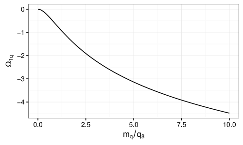
Figure 1: Quark-mass effects $\Omega_{1q}(m_{q}/q_{8})$ as in Eq. (34).

3 Results

3.1 Action density at three-loop level

We write the result for the vacuum expectation value of the action density as

$$\begin{split}\langle E(t)\rangle=\frac{3\alpha_{s}}{4\pi t^{2}}\,\frac{N_{A}}{8}\,K_{E}(\alpha_{s})\,,\end{split}$$ (36)

with the NNLO correction factor

$$\begin{split}K_{E}(\alpha_{s})&=1+\alpha_{s}\,k_{1}+\alpha_{s}^{2}\,k_{2}\,,\end{split}$$ (37)

where $\alpha_{s}\equiv\alpha_{s}^{(n_{f})}(\mu)$ is the strong coupling renormalized at the scale $\mu$ with $n_{f}$ active quark flavors (assumed massless), and $N_{A}$ is the dimension of the adjoint representation of the underlying gauge group ($N_{A}=8$ in QCD). Setting $\mu=1/\sqrt{8t}$, the perturbative coefficients read

$$\begin{split}k_{1}&=8\cdot(0.045741114\,C_{A}+0.001888798\,T_{R}n_{f})-T_{R}\sum_{q}\frac{\Omega_{1q}}{3\pi}\\[-10.00002pt] &\stackrel{{\scriptstyle\text{{QCD}}{}}}{{\approx}}1.098+0.008\,n_{f}+{\cal O}(m_{q}^{2}t)\,,\\[10.00002pt] k_{2}&=8\cdot(-0.0136423(7)\,C_{A}^{2}\\ &\quad+T_{R}n_{f}\,\left(0.006440134(5)\,C_{F}-0.0086884(2)\,C_{A}\right)\\ &\quad+T_{R}^{2}n_{f}^{2}\,0.000936117)\\ &\stackrel{{\scriptstyle\text{{QCD}}}}{{\approx}}-0.982-0.070\,n_{f}+0.002\,n_{f}^{2}\,.\end{split}$$ (38)

The NLO coefficient $k_{1}$ has been obtained analytically for $m_{q}=0$ in Ref.[Luscher:2010iy]; we add mass effects $\Omega_{1q}$ obtained in Eq. (34). However, for most of our analysis, we find that these terms are numerically irrelevant, and we will neglect them unless stated otherwise. The NNLO coefficient $k_{2}$ is the main result of our paper. Similar to Eq. (20), the numbers in brackets denote the numerical uncertainty. The $n_{f}^{2}$-term in $k_{2}$ is completely determined by the two-loop gluon propagator, given analytically in Eq. (26). Similar to $k_{1}$, we simply quote the first few digits of its numerical value. Although our main focus is on QCD, we expressed the result of Eqs. (37,38) in terms of “color” factors of a general simple Lie group (see above). For illustration, we also inserted their QCD values and find very well-behaved perturbative coefficients for any realistic value of $n_{f}$.

The expression of $t^{2}\langle E(t)\rangle$ for general values of the renormalization scale $\mu$ is easily reconstructed using Eq. (23). Fig. 4 shows the variation with this unphysical scale for various values of

$$\begin{split}q_{8}\equiv 1/\sqrt{8t}\,.\end{split}$$ (39)

From the input value $\alpha_{s}^{(5)}(m_{Z})=0.118$, we proceed as described in Fig. 2 in order to derive $\alpha_{s}^{(n_{f})}(q_{8})$. Here, $l$-loop running of $\alpha_{s}$ means that we numerically solve Eq. (23) including the coefficients $\beta_{0},\ldots,\beta_{l-1}$. The decoupling of heavy quarks is consistently performed at $(l-1)$-loop order at the matching scales $\mu_{b}=m_{b}=4.78$ GeV for $\alpha_{s}^{(5)}\to\alpha_{s}^{(4)}$, and $\mu_{b}=2m_{c}=2\cdot 1.67$ GeV for $\alpha_{s}^{(4)}\to\alpha_{s}^{(3)}$ (see Refs.[Chetyrkin:2000yt, Harlander:2002ur] for more details, for example). These start values are then further evolved for fixed $n_{f}$ at the corresponding loop order in order to produce the plots: for the LO/NLO/NNLO result, we apply one/two/three-loop running of $\alpha_{s}$.

Figure 2: Evolution of $\alpha_{s}$ from the input value $\alpha_{s}^{(5)}(m_{Z})$. Solid arrows denote four-loop RG evolution, dashed arrows three-loop decoupling of heavy quarks.

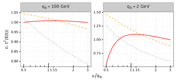
Figure 3: $t^{2}\langle E(t)\rangle$ for $n_{f}=3$ as a function of $\mu/q_{8}$ for $q_{8}=100$ GeV and $q_{8}=2$ GeV at LO (black dotted), NLO (orange dashed), and NNLO (red solid). All curves are normalized to the NNLO-result at $\mu=3q_{8}$. Note the different scales in the two plots.

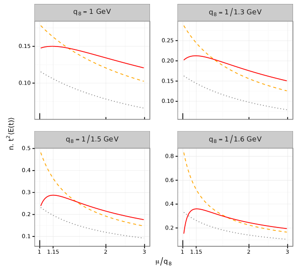
Figure 4: Same as Fig. 3, but for lower values of $q_{8}$, and restricted to the interval $\mu\in[q_{8},3q_{8}]$.

Fig. 3 shows the dependence of $t^{2}\langle E(t)\rangle$ as a function of $\mu/q_{8}$ for $q_{8}=100$ GeV and $q_{8}=2$ GeV. In both cases, one observes a sound perturbative behavior in the interval $\mu\in[q_{8},3q_{8}]$. In addition, the $\mu$-dependence decreases significantly with increasing loop order. These features quickly fade away when going to lower values of $\mu$. Our conclusion is that the best prediction for $t^{2}\langle E(t)\rangle$ is obtained within the $\mu$-interval $[q_{8},3q_{8}]$; its variation within this interval will be used as an estimate of the theoretical uncertainty. Values of $\mu$ outside this interval will be disregarded in what follows.

Fig. 4 shows $t^{2}\langle E(t)\rangle$ within this interval for a few values of $q_{8}\leq 1$ GeV. It is interesting to note that for $q_{8}=1/1.5$ GeV, corresponding to $\sqrt{t}\approx 0.1$ fm, we may still make quantitative predictions when focussing on the $\mu$-interval identified above. For lower energies, the uncertainty at NNLO becomes of the order of 100%, and the NLO and NNLO correction are of the same order of magnitude.

A common feature of all the plots in Figs. 3 and 4 (except the one at $q_{8}=1/1.6$ GeV, a value which we will not consider any further in this paper) is that, within $\mu\in[q_{8},3q_{8}]$, the maximum is quite precisely at $\mu=1.15\,q_{8}$, while the minimum is at $\mu=3q_{8}$. Therefore, the error interval of $t^{2}\langle E(t)\rangle$ as defined above is given to a very good approximation by its values at $\mu=\mu_{-}\equiv 3q_{8}$ and $\mu=\mu_{+}\equiv 1.15q_{8}$.

Fig. 5 shows the dependence of $t^{2}\langle E(t)\rangle$ on $\sqrt{8t}=1/q_{8}$ for $n_{f}=3$ active flavors at LO, NLO, and NNLO, with error bands evaluated as indicated above. For each value of $q_{8}$, the strong coupling $\alpha_{s}$ is evolved at four-loop level from $\alpha_{s}^{(5)}(m_{Z})$ to $\alpha_{s}^{(3)}(q_{8})$ (including three-loop matching at the quark thresholds), and subsequently at the pertinent order from $\alpha_{s}^{(3)}(q_{8})$ to $\alpha_{s}^{(3)}(\mu)$, with $\mu=1.15q_{8}$ and $\mu=3q_{8}$ for the upper and lower edge of the uncertainty band, respectively. One observes that the resulting NLO and the NNLO bands nicely overlap, which gives confidence in using these bands as measures of the theoretical uncertainty. There is hardly any overlap of these curves with the LO band though.

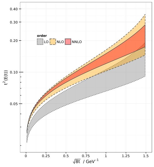
Figure 5: $t^{2}\langle E(t)\rangle$ for $n_{f}=3$ as a function of $\sqrt{8t}$ (in GeV^-1) for $\mu=3/\sqrt{8t}$ (lower) and $\mu=1.15/\sqrt{8t}$ (upper) at LO (gray), NLO (orange), and NNLO (red).

3.2 Extracting $\alpha_{s}(m_{Z})$

One of the most interesting applications of our results would be the derivation of a numerical value of $\alpha_{s}(m_{Z})\equiv\alpha_{s}^{(5)}(m_{Z})$ using lattice data as input. This will be most promising, of course, if the lattice calculation for $t^{2}\langle E(t)\rangle$ could be extended to the perturbative regime, which seems to have become a realistic perspective [Luscher:2014kea].

Assume that a lattice value $e(t)$ for $t^{2}\langle E(t)\rangle$ is known, evaluated at $t=1/(8q_{8}^{2})$ and for $n_{f}$ active quark flavors. Using the perturbative result of Eqs. (36) and (37) through order $l$ (including its $\mu$-dependence), one can derive an $l$-loop value for $\alpha_{s}^{(n_{f})}(\mu)$, which can then be converted into a value for $\alpha_{s}^{(5)}(m_{Z})$ through four-loop RG evolution and three-loop matching to the $n_{f}=5$ theory. Table 3 shows this relation at NNLO (i.e. for $l=3$) for a number of values of $q_{8}$ and $n_{f}$. The values of $t^{2}\langle E(t)\rangle$ given in that table correspond to the center of the error band, i.e., they are the arithmetic means of $t^{2}\langle E(t)\rangle$ evaluated at $\mu=1.15\,q_{8}$ and $\mu=3\,q_{8}$. These numbers take into account the NLO quark effects given in Eq. (34), whereupon the lightest three quark flavors are taken massless, while $m_{c}=1.67$ GeV and $m_{b}=4.78$ GeV. The mass effects therefore only affect the columns with $n_{f}\geq 4$. At $q_{8}=2$ GeV, their effect on $t^{2}\langle E(t)\rangle$ is about 0.8%, at $q_{8}=10$ GeV it is less than 0.3% both for $n_{f}=4$ and $n_{f}=5$, while at $q_{8}=m_{Z}$, they have no effect on the digits given in the table.

	$t^{2}\langle E(t)\rangle\cdot 10^{4}$
$q_{8}$	2 GeV		10 GeV			$m_{Z}$
$\alpha_{s}(m_{Z})$	$n_{f}=3$	$n_{f}=4$	$n_{f}=3$	$n_{f}=4$	$n_{f}=5$	$n_{f}=3$	$n_{f}=4$	$n_{f}=5$
0.113	744	755	424	446	456	267	285	299
0.1135	753	764	426	449	459	268	286	301
0.114	762	773	429	452	462	269	287	302
0.1145	771	782	432	455	466	270	289	303
0.115	780	792	435	458	469	272	290	305
0.1155	789	802	438	461	472	273	291	306
0.116	798	811	440	465	476	274	292	308
0.1165	808	821	443	468	479	275	294	309
0.117	818	832	446	471	483	276	295	311
0.1175	827	842	449	474	486	277	296	312
0.118	837	852	452	478	490	278	298	314
0.1185	847	863	455	481	493	279	299	315
0.119	858	874	457	484	497	280	300	316
0.1195	868	885	460	488	500	281	301	318
0.12	879	896	463	491	504	282	303	319

Table 3: Numerical values for $10^{4}\cdot t^{2}\langle E(t)\rangle$ corresponding to various $\alpha_{s}(m_{Z})\equiv\alpha_{s}^{(5)}(m_{Z})$. Given a numerical result for $t^{2}\langle E(t)\rangle$ (e.g., from a lattice calculation), this table lets one deduce the corresponding value of $\alpha_{s}(m_{Z})$. The associated perturbative uncertainty for $n_{f}=5$ and $n_{f}=3$ can be read off from Fig. 6.

In accordance with our previous considerations, we estimate the theoretical accuracy of this extraction by considering $t^{2}\langle E(t)\rangle$ at $\mu=1.15\,q_{8}$ and $3\,q_{8}$ when deriving $\alpha_{s}^{(n_{f})}(\mu)$ from $e(t)$. The result for $n_{f}=3$ is shown in Fig. 6. In lack of a precise value of $e(t)$ at sufficiently large $q_{8}$, we substitute it by the perturbative NNLO expression for $t^{2}\langle E(t)\rangle$ at $\mu=q_{8}$, where the numerical value for $\alpha_{s}^{(3)}(q_{8})$ is derived by three-loop running and two-loop matching ($\mu_{b}=m_{b}$ and $\mu_{c}=2m_{c}$) from the input value $\alpha_{s}(m_{Z})=0.118$. Therefore, the NNLO band for $\alpha_{s}(m_{Z})$ in the upper part of Fig. 6 always includes the value 0.118 by construction. Similar to Fig. 5, the width of the bands decreases remarkably towards higher orders of perturbation theory. The NNLO band lies completely within the NLO band, while LO has no overlap with NLO.

The lower part of the figure shows the theoretical accuracy that could be achieved by such an analysis, derived by taking the relative width of the bands of the upper part of the plot,

$$\begin{split}\frac{\Delta\alpha_{s}}{\alpha_{s}}=\frac{\alpha_{s}^{\text{max}}(m_{Z})-\alpha_{s}^{\text{min}}(m_{Z})}{\alpha_{s}^{\text{max}}(m_{Z})+\alpha_{s}^{\text{min}}(m_{Z})}\,.\end{split}$$ (40)

For example, if $e(t)$ is given only at $t=1/(8\text{GeV}^{2})$, the NNLO uncertainty on $\alpha_{s}(m_{Z})$ would be around $2.5\%$. On the other hand, knowning $e(t)$ at $t=1/(8m_{Z}^{2})$ would allow one to derive $\alpha_{s}(m_{Z})$ to $0.5\%$ accuracy which is at the same level as the current world average on this quantity [Agashe:2014kda]. Also shown in the lower plot is the uncertainty which results from knowing $e(t)$ for $n_{f}=5$ active flavors (lower dotted red line). In this case, the numbers above decrease to $\sim 1.1\%$ and $\sim 0.3\%$, respectively, because of the lower value of the QCD $\beta$ function.

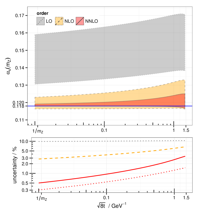
Figure 6: Upper plot: numerical value for $\alpha_{s}^{(5)}(m_{Z})$ derived at LO (gray), NLO (orange), and NNLO (red) from a hypothetical exact value of $t^{2}\langle E(t)\rangle|_{n_{f}=3}$ (see main text for details). Lower plot: corresponding theoretical uncertainty (see Eq. (40)). The red dotted line in the lower plot shows the uncertainty when the analysis is based on $t^{2}\langle E(t)\rangle|_{n_{f}=5}$.

3.3 Derivative of the action density

In Ref.[Borsanyi:2012zs] it was argued that the quantity

$$\begin{split}W(t)\equiv t\frac{\text{d}}{\text{d}t}t^{2}\langle E(t)\rangle\end{split}$$ (41)

is more suitable for scale setting on the lattice. Neglecting again quark-mass effects, $t$ and $\mu$ are the only dimensional scales of the dimensionless quantity $t^{2}\langle E(t)\rangle$, so that the dependence on them can only be in terms of $l_{t\mu}\equiv\ln t\mu^{2}$. Using Eq. (21), we can thus write

$$\begin{split}W(t)=\frac{\partial}{\partial l_{t\mu}}t^{2}\langle E(t)\rangle=-\alpha_{s}\beta(\alpha_{s})\frac{\partial}{\partial\alpha_{s}}t^{2}\langle E(t)\rangle\,,\end{split}$$ (42)

with the $\beta$ function defined in Eq. (22). The result is therefore

$$\begin{split}W(t)&=\frac{3}{4}\left(\frac{\alpha_{s}}{\pi}\right)^{2}\beta_{0}\left[1+\alpha_{s}\left(b_{1}+2k_{1}\right)+\alpha_{s}^{2}\left(b_{2}+2\,b_{1}k_{1}+3k_{2}\right)\right]\,,\end{split}$$ (43)

with $k_{1}$, $k_{2}$ given in Eq. (37), $b_{n}\equiv\beta_{n}/(\pi^{n}\beta_{0})$, where $\beta_{0}$ and $\beta_{1}$ have been given in Eq. (24), and

$$\begin{split}\beta_{2}=\frac{2857}{128}-\frac{5033}{1152}\,n_{f}+\frac{325}{3456}\,n_{f}^{2}\,.\end{split}$$ (44)

Numerically, this gives, for QCD and setting $\mu=1/\sqrt{8t}$,

$$\begin{split}W(t)&=\alpha_{s}^{2}\,\left(0.208975-0.0126651\,n_{f}\right)\\ &+\alpha_{s}^{3}\left(0.613022-0.0437989\,n_{f}-0.000191375\,n_{f}^{2}\right)\\ &+\alpha_{s}^{4}\,\left(-0.10538(3)-0.0798618(4)\,n_{f}+0.00426484(9)\,n_{f}^{2}-0.0000711364\,n_{f}^{3}\right)\,.\end{split}$$ (45)

Again, the $\mu$-dependent terms can be easily reconstructed using renormalization group invariance.

Performing a similar analysis for $W(t)$ as done in the preceeding sections for $t^{2}\langle E(t)\rangle$, we see no improvement concerning the precision for the extraction of $\alpha_{s}$ relative to the one based on $t^{2}\langle E(t)\rangle$.

4 Conclusions and Outlook

The action density for QCD gradient flow fields has been evaluated at three-loop level. The perturbative expansion has been derived by standard Wick contractions, and the resulting integrals have been solved by sector decomposition supplied by a suitable numerical integration algorithm. A number of strong checks on the result has been performed. In addition, quark-mass effect have been included at NLO.

Our NNLO coefficient indicates a very well-behaved perturbative series for the action density down to energy scales of about $q_{8}\sim 0.65$ GeV, corresponding to $\sqrt{t}\sim 0.11$ fm. This seems well within reach of a direct comparison to a lattice evaluation of $t^{2}\langle E(t)\rangle$. Given that $t^{2}\langle E(t)\rangle$ can be evaluated independently (e.g. by a lattice calculation) at sufficiently large values of the flow time with high precision, one may derive a numerical value for $\alpha_{s}(m_{Z})$ by comparison to the perturbative result. We provide an estimate of the resulting uncertainty and find that it could be competitive with the current world average.

On the perturbative side, further steps could be the development of more efficient tools for the evaluation of the integrals, the consideration of other observables, or the application of the flow-field formalism to quark fields as introduced in Ref.[Luscher:2013cpa].

Finally, it should be noted that there is no conceptual limitation of the calculational method described in this paper which would restrict it to the three-loop level. In the current implementation, however, an extension to four loops would require a significant increase in the computing resources.

Acknowledgments.

We are particularly obliged to Zoltan Fodor for initiating and motivating this work, to Martin Lüscher for providing us with private notes on Ref.[Luscher:2010iy], to Szabolcs Borsányi, Christian Hölbling, and Rainer Sommer for helpful communication, and to Marisa Sandhoff and Torsten Harenberg for administration of the DFG FUGG cluster at Bergische Universität Wuppertal, where most of the calculations for this paper were performed.

References

- [1] H. Fritzsch, M. Gell-Mann and H. Leutwyler, Advantages of the Color Octet Gluon Picture, Phys. Lett. B 47 (1973) 365.
- [2] H.D. Politzer, Reliable Perturbative Results For Strong Interactions?, Phys. Rev. Lett. 30 (1973) 1346.
- [3] D.J. Gross and F. Wilczek, Ultraviolet Behavior Of Non-Abelian Gauge Theories, Phys. Rev. Lett. 30 (1973) 1343.
- [4] K.G. Wilson, Confinement of Quarks, Phys. Rev. D 10 (1974) 2445.
- [5] G. Martinelli, C. Pittori, C.T. Sachrajda, M. Testa, and A. Vladikas, A General method for nonperturbative renormalization of lattice operators, Nucl. Phys. B 445 (1995) 81