The two-loop energy-momentum tensor within the gradient-flow formalism

Abstract

The gradient-flow formulation of the energy-momentum tensor of QCD is extended to NNLO perturbation theory. This means that the Wilson coefficients which multiply the flowed operators in the corresponding expression for the regular energy-momentum tensor are calculated to this order. The result has been obtained by applying modern tools of regular perturbation theory, reducing the occurring two-loop integrals, which also include flow-time integrations, to a small set of master integrals which can be calculated analytically.

1 Introduction

The gradient-flow formalism as introduced by Lüscher [1] and further formalized by Lüscher and Weisz [Luscher:2011bx] has proven useful in lattice QCD in many respects. One of its main virtues is that composite operators at finite flow time $t$ do not require ultra-violet (UV) renormalization beyond the one of the involved parameters and fields. This means that the operators do not mix under renormalization-group running, which makes it particularly simple to combine results from different regularization schemes. This feature opens promising prospects for a cross-fertilization of lattice and perturbative calculations, such as a possible lattice determination of $\alpha_{s}(M_{Z})$, for example [Harlander:2016vzb].

A particularly powerful way to exhibit this possible interplay is obtained by considering the expansion of composite operators in the limit of small flow time, which expresses flowed operators in terms of QCD operators at $t=0$, with $t$-dependent Wilson coefficients [Luscher:2011bx]. This method has been used by Makino and Suzuki [Suzuki:2013gza, Makino:2014taa] to derive a regularization-independent formula for the energy-momentum tensor (EMT) $T_{\mu\nu}$ which has already led to promising results (see, e.g., Refs. [Asakawa:2013laa, Kitazawa:2016dsl, Taniguchi:2016ofw, Kitazawa:2017qab, Yanagihara:2018qqg]).

The universal Wilson coefficients that occur in the formula of Ref. [Makino:2014taa] for the EMT have been calculated through next-to-leading order (NLO) in perturbation theory [Suzuki:2013gza, Makino:2014taa]. This corresponds to a one-loop calculation in the sense that it involves integrals over a single $D$-dimensional momentum. In this paper, we will carry this calculation to the next perturbative order. It is important to note at this point that the integrals which occur in the gradient-flow formalism are of a more general type than in regular QCD. They involve additional exponential factors which depend on loop and external momenta, as well as on flow-time variables, some of which are also integrated over. Nevertheless, the first two-loop result was already obtained in Ref. [1], even in analytic form. The extension to the three-loop level required significant aid from computer algebra and numerical tools [Harlander:2016vzb]. From the quantum-field theoretical point of view, it closely followed the steps of Ref. [1] by directly expressing the Green’s functions in terms of integrals with the help of Wick’s theorem. The integrals themselves were evaluated using sector-decomposition [Binoth:2003ak, Smirnov:2013eza] in order to isolate the poles in $D-4$, whose coefficients were determined using high-precision numerical methods [genz, holodborodko].

In the current calculation, we apply a completely independent setup. On the one hand, it applies the gradient-flow formalism described in terms of a five-dimensional quantum field theory [Luscher:2011bx], which leads to well-defined, albeit non-standard Feynman rules. On the other hand, rather than evaluating the resulting integrals numerically, we express them in terms of master integrals using the integration-by-parts method of Chetyrkin and Tkachov [Chetyrkin:1981qh]. This reduces the NLO calculation of the Wilson coefficients of the EMT to a single one-loop integral without flow-time integration. The next-to-next-to-leading order (NNLO) calculation leads to four two-loop master integrals without flow-time integration, and two two-loop master integrals with a single flow-time integration. All master integrals can be calculated analytically by standard means for general values of $D$, the number of space-time dimensions.

By suitable renormalization, the Wilson coefficients of the EMT can be defined in such a way that they are formally renormalization-scale independent. For a fixed-order perturbative result, this means that the renormalization-scale dependence is formally of higher order. This allows one to estimate the perturbative uncertainty on the Wilson coefficients through their residual dependence on the renormalization scale $\mu$ around a particular “central” value. Based on the form of the analytical result, we argue for a specific choice of this central value. Our numerical study shows that the higher-order terms indeed lead to an appreciable reduction of the $\mu$-variation. However, by comparison of the successive higher-order terms, it appears that the uncertainty estimate from a variation within $\mu\in[\mu_{0}/2,2\mu_{0}]$, as it is common practice in regular perturbative QCD calculation, might be too optimistic.

While we consider the NNLO expressions for the Wilson coefficients of the EMT as our main result, our calculation allows us to obtain a number of additional results that might be useful in a broader context. Among these are the flowed quark-field renormalization constant $Z_{\chi}$, and the matrix of anomalous dimensions for the set of operators which form the energy-momentum tensor in regular (non-flowed) QCD through NNLO.

The remainder of the paper is structured as follows. After briefly introducing the perturbative gradient-flow formalism in order to define our notation in Sect. 2, we outline the approach of Refs. [Suzuki:2013gza, Makino:2014taa] for using this formalism to define the EMT in Sect. 3. Technical details of our calculation are described in Sect. 4. Section 5 contains our main result, the Wilson coefficients through NNLO QCD in the $\overline{\mbox{{MS}}}$ scheme. As pointed out in Ref. [Makino:2014taa], the trace anomaly of the EMT allows for a welcome check of the calculation; we briefly describe the derivation of the resulting relations among the coefficient functions in Sect. 6. Finally, in Sect. 7, we use the finiteness condition of the flowed operators in order to derive the anomalous-dimension matrix for the set of operators which occur in the EMT in regular QCD. Section 8 presents our conclusions.

2 QCD gradient flow in perturbation theory

In the following, we will work in $D$-dimensional Euclidean space-time with $D=4-2\epsilon$. The gradient-flow formalism continues the gluon and quark fields $A^{a}_{\mu}(x)$ and $\psi(x)$ of regular QCD to $(D+1)$-dimensional fields $B^{a}_{\mu}(t,x)$ and $\chi(t,x$) through the boundary conditions

$$\begin{split}B_{\mu}^{a}(t=0,x)=A_{\mu}^{a}(x)\,,\qquad\chi(t=0,x)=\psi(x)\,,\end{split}$$ (1)

and the flow equations

$$\begin{split}\partial_{t}B_{\mu}^{a}&=\mathcal{D}^{ab}_{\nu}G_{\nu\mu}^{b}+\kappa\mathcal{D}^{ab}_{\mu}\partial_{\nu}B_{\nu}^{b}\,,\\ \partial_{t}\chi&=\Delta\chi-\kappa\partial_{\mu}B_{\mu}^{a}T^{a}\chi\,,\\ \partial_{t}\overline{\chi}&=\overline{\chi}\overleftarrow{\Delta}+\kappa\overline{\chi}\partial_{\mu}B_{\mu}^{a}T^{a}\,,\end{split}$$ (2)

where the “flow time” $t$ is a parameter of mass dimension minus two, and $\kappa$ is an additional gauge parameter which drops out of physical observables.

The $(D+1)$-dimensional field-strength tensor is defined as

$$G_{\mu\nu}^{a}=\partial_{\mu}B_{\nu}^{a}-\partial_{\nu}B_{\mu}^{a}+f^{abc}B_{\mu}^{b}B_{\nu}^{c}\,,$$ (3)

the covariant derivative in the adjoint representation is given by

$$\mathcal{D}_{\mu}^{ab}=\delta^{ab}\partial_{\mu}-f^{abc}B_{\mu}^{c}\,,$$ (4)

and

$$\begin{split}\Delta=(\partial_{\mu}+B_{\mu})(\partial_{\mu}+B_{\mu})\,,\qquad\overleftarrow{\Delta}=(\overleftarrow{\partial}\!_{\mu}-B_{\mu})(\overleftarrow{\partial}\!_{\mu}-B_{\mu})\,.\end{split}$$ (5)

As usual, the color indices of the adjoint representation are denoted by $a,b,c,\ldots$, while $\mu,\nu,\rho,\ldots$ are $D$-dimensional Lorentz indices. Color indices of the fundamental representation are suppressed throughout this paper, unless required by clarity. The symmetry generators $T^{a}$ obey the commutation relation

$$\begin{split}[T^{a},T^{b}]=f^{abc}T^{c}\,,\end{split}$$ (6)

with the structure constants $f^{abc}$.

The flow-field equation leads to a smearing of gauge-field configurations at finite flow time $t>0$. As a consequence, composite operators at $t>0$ do not require renormalization beyond the renormalization of the parameters and fields of the Lagrangian. For the strong coupling and the quark mass, the renormalization constants are identical to those at $t=0$; the flowed gluon fields do not require renormalization at finite flow time as was pointed out in Ref. [Luscher:2011bx]. The renormalization constant for the flowed quark field through NNLO is a by-product of this paper and will be given below.

3 Energy-momentum tensor

In a continuous $D$-dimensional space-time, the gauge invariant part of the EMT reads

$$\begin{split}T_{\mu\nu}(x)\equiv\frac{1}{g_{0}^{2}}\left[\mathcal{O}_{1,\mu\nu}(x)-\frac{1}{4}\mathcal{O}_{2,\mu\nu}(x)\right]+\frac{1}{4}\mathcal{O}_{3,\mu\nu}(x)-\frac{1}{2}\mathcal{O}_{4,\mu\nu}(x)-\mathcal{O}_{5,\mu\nu}(x)\,,\end{split}$$ (7)

where $g_{0}$ is the bare coupling constant of QCD. The operators are defined as

$$\begin{split}\mathcal{O}_{1,\mu\nu}(x)&\equiv F_{\mu\rho}^{a}(x)F_{\nu\rho}^{a}(x)\,,\\[10.0pt] \mathcal{O}_{2,\mu\nu}(x)&\equiv\delta_{\mu\nu}F_{\rho\sigma}^{a}(x)F_{\rho\sigma}^{a}(x)\,,\\[10.0pt] \mathcal{O}_{3_{f},\mu\nu}(x)&\equiv\bar{\psi}_{f}(x)\left(\gamma_{\mu}\overleftrightarrow{D}\!_{\nu}+\gamma_{\nu}\overleftrightarrow{D}\!_{\mu}\right)\psi_{f}(x)\,,\\ \mathcal{O}_{4_{f},\mu\nu}(x)&\equiv\delta_{\mu\nu}\bar{\psi}_{f}(x)\overleftrightarrow{\not{D}}\psi_{f}(x)\,,\phantom{\bigg{(}\bigg{)}}\\ \mathcal{O}_{5_{f},\mu\nu}(x)&\equiv\delta_{\mu\nu}m_{f,0}\bar{\psi}_{f}(x)\psi_{f}(x)\,,\\ \mathcal{O}_{i,\mu\nu}(x)&=\sum_{f=1}^{n_{F}}\mathcal{O}_{i_{f},\mu\nu}(x)\,,\qquad i\in\{3,4,5\}\,,\end{split}$$ (8)

where $f$ labels the $n_{F}$ different quark flavors, $m_{f,0}$ is the bare quark mass, and

$$\begin{split}F^{a}_{\mu\nu}=\partial_{\mu}A_{\nu}^{a}-\partial_{\nu}A_{\mu}^{a}+f^{abc}A_{\mu}^{b}A_{\nu}^{c}\,,\qquad\overleftrightarrow{D}\!_{\mu}=\partial_{\mu}-\overleftarrow{\partial}\!_{\mu}+2A_{\mu}\,.\end{split}$$ (9)

The notation $i_{f}\in\{i_{1},\ldots,i_{n_{F}}\}$ for the indices which label different flavors will be useful later on in this paper. In general, $T_{\mu\nu}$ may contain gauge-dependent operators  which vanish when evaluating physical matrix elements [Nielsen:1977sy]. Here and in what follows, we implicitly assume that the vacuum expectations values of all composite operators have been subtracted so that $\langle\mathcal{O}_{i,\mu\nu}(x)\rangle\equiv 0\ \forall i$.

In this paper, we will focus on the case where physical matrix elements of the EMT itself are considered, i.e. no other operator multiplies the EMT at the same space-time point. In this case, the equations-of-motion (EOM) render the set of operators in Eq. (8) redundant. In particular, the EOM for the quark fields in regular QCD implies

$$0=\mathcal{O}_{4,\mu\nu}(x)+2\,\mathcal{O}_{5,\mu\nu}(x)\,,$$ (10)

which allows us to eliminate $\mathcal{O}_{5,\mu\nu}$ from the set of operators in Eq. (8). Note that due to this relation, the last two terms in Eq. (7) cancel.

We will further assume all quark masses to be equal to each other

$$m_{f,0}=m_{0}\,,\qquad f=1,\ldots,n_{F}\,.$$ (11)

Therefore, the different quarks are indistinguishable and the mixing between two different quark flavors cannot depend on the flavors.

Defining the analogous operators of Eq. (8) for flowed fields, we write

$$\begin{split}\tilde{\mathcal{O}}_{1,\mu\nu}(t,x)&\equiv G_{\mu\rho}^{a}(t,x)G_{\nu\rho}^{a}(t,x)\,,\\[10.0pt] \tilde{\mathcal{O}}_{2,\mu\nu}(t,x)&\equiv\delta_{\mu\nu}G_{\rho\sigma}^{a}(t,x)G_{\rho\sigma}^{a}(t,x)\,,\\[10.0pt] \tilde{\mathcal{O}}_{3_{f},\mu\nu}(t,x)&\equiv Z_{\chi_{f}}\bar{\chi}_{f}(t,x)\left(\gamma_{\mu}\overleftrightarrow{\mathcal{D}}\!_{\nu}+\gamma_{\nu}\overleftrightarrow{\mathcal{D}}\!_{\mu}\right)\chi_{f}(t,x)\,,\\ \tilde{\mathcal{O}}_{4_{f},\mu\nu}(t,x)&\equiv Z_{\chi_{f}}\delta_{\mu\nu}\bar{\chi}_{f}(t,x)\overleftrightarrow{\not{\mathcal{D}}}\chi_{f}(t,x)\,,\\ \tilde{\mathcal{O}}_{i,\mu\nu}&=\sum_{f=1}^{n_{F}}\tilde{\mathcal{O}}_{i_{f},\mu\nu}\,,\qquad i\in\{3,4\}\,,\end{split}$$ (12)

where $Z_{\chi_{f}}\equiv Z_{\chi}$ is the renormalization constant for the flowed quark fields, and

$$\begin{split}\overleftrightarrow{\mathcal{D}}\!_{\mu}=\partial_{\mu}-\overleftarrow{\partial}\!_{\mu}+2B_{\mu}\,.\end{split}$$ (13)

Since we have eliminated $\mathcal{O}_{5,\mu\nu}$ from the set of operators by using Eq. (10), we do not need to include a flowed version of this operator in Eq. (12). Similar to the composite operators of regular QCD, we assume that the vacuum expectation values of the flowed composite operators have been subtracted, i.e. $\langle\tilde{\mathcal{O}}_{i,\mu\nu}(t,x)\rangle\equiv 0\ \forall i$.

We can now use the expansion in small flow time [Luscher:2011bx]

$$\begin{split}\tilde{\mathcal{O}}_{i,\mu\nu}(t,x)=\zeta_{ij}(t)\mathcal{O}_{j,\mu\nu}(x)+\ldots\,,\end{split}$$ (14)

to get a relation between flowed and regular QCD operators. In Eq. (14), and similarly in what follows, a sum $\sum_{j=1}^{4}$ is understood. The ellipsis denotes terms that vanish as $t\to 0$ which will be neglected throughout this paper. As discussed above, matrix elements of the l.h.s. of this equation are finite after renormalization of the QCD parameters, while those of the regular QCD operators on the r.h.s. are in general divergent. The mixing matrix $\zeta_{ij}(t)$ will therefore be divergent as well.

Inverting Eq. (14) and using it to re-express the regular QCD operators in the energy-momentum tensor in terms of flowed fields, one arrives at

$$\begin{split}T_{\mu\nu}(x)=c_{i}(t)\tilde{\mathcal{O}}_{i,\mu\nu}(t,x)\,,\end{split}$$ (15)

where

$$\begin{split}c_{i}(t)\equiv\frac{1}{g_{0}^{2}}\left(\zeta_{1i}^{-1}(t)-\frac{1}{4}\zeta_{2i}^{-1}(t)\right)+\frac{1}{4}\zeta_{3i}^{-1}(t)\,,\qquad i=1,\ldots,4\,.\end{split}$$ (16)

Since matrix elements of the $\tilde{\mathcal{O}}_{i}$ as well as the energy-momentum tensor itself are finite (after mass and charge renormalization), the universal coefficients $c_{i}(t)$ of Eq. (16) are finite as well. In Ref. [Makino:2014taa], they have been calculated in perturbation theory through NLO QCD. The goal of the current paper is to evaluate them through NNLO QCD.

4 Calculation of the Wilson coefficients

4.1 Method of Projectors

To compute the coefficients $\zeta_{ij}(t)$ we use the so-called “method of projectors” [Gorishnii:1983su, Gorishnii:1986gn], which consists of constructing external states $|k\rangle$ and differential operators $D_{k}$ for which

$$\begin{split}P_{k}[\mathcal{O}_{i}(x)]\equiv D_{k}\langle 0|\mathcal{O}_{i}(x)|k\rangle=\delta_{ik}\,,\end{split}$$ (17)

where we have dropped the Lorentz indices for convenience, and we define the matrix element to include only diagrams which are one-particle irreducible (1PI) with respect to (w.r.t.) QCD particles. Applying $P_{k}$ on both sides of Eq. (14), one obtains

$$\begin{split}P_{k}[\tilde{\mathcal{O}}_{i}(t,x)]=\zeta_{ij}(t)P_{k}[\mathcal{O}_{j}(x)]\,.\end{split}$$ (18)

Since the $\zeta_{ij}(t)$ only depend on the flow time $t$ and the renormalization scale $\mu$, we can choose arbitrary values for all other dimensional parameters in this equation. Setting them to zero turns all higher-order corrections on the r.h.s. into massless tadpoles, so that Eq. (17) is only required to hold at tree-level. One thus obtains

$$\begin{split}\zeta_{ij}(t)=P_{j}[\tilde{\mathcal{O}}_{i}(t,x)]\Big{|}_{p=m=0}\,,\end{split}$$ (19)

where $m$ and $p$ collectively denote all masses and external momenta. The right-hand side thus results in vacuum diagrams whose only dimensional scale is $t$.

In order to find suitable projectors, we first derive the Feynman rules for the relevant terms of the operators. For example,

$$\mathcal{O}_{1,\mu\nu} =\partial_{\mu}A_{\rho}^{c}\partial_{\nu}A_{\rho}^{c}+\cdots \Rightarrow \begin{gathered}\includegraphics{dias/O1.pdf}\end{gathered}=-p_{1,\mu}p_{2,\nu}\delta_{\alpha\beta}\delta^{ab},$$ (21)

where the momenta are defined to be outgoing. This suggests to use

$$\begin{split}P_{1}[X]=-\frac{\delta^{ab}}{N_{A}}P_{\alpha\beta|\rho\mu|\sigma\nu}\frac{\partial}{\partial p_{1,\rho}}\frac{\partial}{\partial p_{2,\sigma}}\langle 0|A_{\alpha}^{a}(p_{1})A_{\beta}^{b}(p_{2})X_{\mu\nu}|0\rangle\,,\end{split}$$ (22)

where $N_{A}$ is the dimension of the adjoint representation of the gauge group; for SU($N_{c}$), it is $N_{A}=N_{c}^{2}-1$. The projector onto the Lorentz structure is defined by

$$\begin{split}P_{\alpha_{1}\beta_{1}|\cdots|\alpha_{n}\beta_{n}}T_{\alpha_{1}\beta_{1}\cdots\alpha_{n}\beta_{n}}=\left\{\begin{array}[]{ll}1\phantom{\Bigg{(}}&\text{for}\quad T_{\alpha_{1}\beta_{1}\cdots\alpha_{n}\beta_{n}}=\delta_{\alpha_{1}\beta_{1}}\cdots\delta_{\alpha_{n}\beta_{n}}\,,\\[3.00003pt] \hbox{\multirowsetup 0}&\text{for any other linearly}\\ &\text{independent Lorentz tensor.}\end{array}\right.\end{split}$$ (23)

In the appendix, one can find the relevant parts of the Feynman rules for the other operators, which in a similar way lead to the projectors

$$\begin{split}P_{2}[X]&=-\frac{\delta^{ab}}{4N_{A}}P_{\alpha\beta|\mu\nu|\rho\sigma}\frac{\partial}{\partial p_{1,\rho}}\frac{\partial}{\partial p_{2,\sigma}}\langle 0|A_{\alpha}^{a}(p_{1})A_{\beta}^{b}(p_{2})X_{\mu\nu}|0\rangle\,,\\ P_{3_{f}}[X]&=-i\frac{\delta^{ij}}{4N_{c}}P_{\rho\mu|\sigma\nu}\frac{\partial}{\partial p_{2,\sigma}}\text{Tr}\left[\gamma_{\rho}\langle 0|\psi_{f}^{j}(p_{2})\bar{\psi}_{f}^{i}(p_{1})X_{\mu\nu}|0\rangle\right]\,,\\ P_{4_{f}}[X]&=-i\frac{\delta^{ij}}{4N_{c}}P_{\mu\nu|\sigma\rho}\frac{\partial}{\partial p_{2,\sigma}}\text{Tr}\left[\gamma_{\rho}\langle 0|\psi_{f}^{j}(p_{2})\bar{\psi}_{f}^{i}(p_{1})X_{\mu\nu}|0\rangle\right]\\ &\qquad-\frac{1}{2}\frac{\delta^{ij}}{4N_{c}}P_{\mu\nu}\frac{\partial}{\partial m_{0}}\text{Tr}\left[\langle 0|\psi_{f}^{j}(p_{2})\bar{\psi}_{f}^{i}(p_{1})X_{\mu\nu}|0\rangle\right]\,,\end{split}$$ (24)

where $N_{c}$ is the dimension of the fundamental representation of the gauge group, i.e. the number of colors, and $i$ and $j$ are the corresponding indices. The trace appearing in the projectors $P_{3_{f}}$ and $P_{4_{f}}$ is taken w.r.t. the spinor indices of the Green’s function, and $f$ denotes the associated quark flavor. Note that $P_{4_{f}}$ is constructed such that

$$\begin{split}P_{4_{f}}[\mathcal{O}_{4}+2\mathcal{O}_{5}]=0\end{split}$$ (25)

in order to ensure that only those fermionic operators are taken into account which do not vanish according to the EOM, see Eq. (10).

With this procedure, we get a mixing matrix which distinguishes between different quark flavors. To avoid confusion with $\zeta_{ij}(t)$, which is the mixing matrix between operators summed over all flavors, we will call it $\Omega_{ij}(t)$. This matrix is then defined by

$$\tilde{\mathcal{O}}_{i,\mu\nu}(t,x)=\Omega_{ij}(t)\mathcal{O}_{j,\mu\nu}(x)\,,$$ (26)

where double indices in this expression are summed over $\{1,2,3_{1},\ldots,3_{n_{F}},4_{1},\ldots,4_{n_{F}}\}$ (see Eq. (8)), in contrast to Eq. (15), where double indices are summed over $\{1,2,3,4\}$. Its general structure is given by

$$\Omega=\begin{pmatrix}\Omega_{11}&\Omega_{12}&\underline{\Omega_{13}}^{T}&\underline{\Omega_{14}}^{T}\\ \Omega_{21}&\Omega_{22}&\underline{\Omega_{23}}^{T}&\underline{\Omega_{24}}^{T}\\ \underline{\Omega_{31}}&\underline{\Omega_{32}}&\underline{\underline{\Omega_{33}}}&\underline{\underline{\Omega_{34}}}\\ \underline{\Omega_{41}}&\underline{\Omega_{42}}&\underline{\underline{\Omega_{43}}}&\underline{\underline{\Omega_{44}}}\end{pmatrix}\,,$$ (27)

where an element $\Omega_{ij}$ represents the mixing between $\mathcal{O}_{i}$ and $\tilde{\mathcal{O}}_{j}$, taking into account individual flavors. Therefore, an underlined and a double underlined element denotes an $n_{F}$-dimensional vector and an $n_{F}\times n_{F}$ dimensional matrix, respectively. Their elements describe the mixing between different flavors. As the quarks are indistinguishable, the $n_{F}$ and $n_{F}^{2}$ dimensional objects appearing in Eq. (27) can each be described by two independent parameters, named $\omega_{ij}$ and $\bar{\omega}_{ij}$:

$$\begin{split}\Omega_{ij}=\omega_{ij}\quad\text{for}\quad i,j<3,\qquad\underline{\Omega_{ij}}=\omega_{ij}\begin{pmatrix}1\\ \vdots\\ 1\end{pmatrix}\quad\text{for}\quad i<3,\ j>2\quad\text{or}\quad i>2,\ j<3\,,\end{split}$$

$$\begin{split}\underline{\underline{\Omega_{ij}}}=\begin{pmatrix}\omega_{ij}&\overline{\omega}_{ij}&\overline{\omega}_{ij}&\dots&\overline{\omega}_{ij}\\ \overline{\omega}_{ij}&\omega_{ij}&\overline{\omega}_{ij}&\dots&\overline{\omega}_{ij}\\ \overline{\omega}_{ij}&\overline{\omega}_{ij}&\omega_{ij}&\dots&\overline{\omega}_{ij}\\ \vdots&\vdots&\vdots&\ddots&\vdots\\ \overline{\omega}_{ij}&\overline{\omega}_{ij}&\overline{\omega}_{ij}&\dots&\omega_{ij}\end{pmatrix}\quad\text{for}\quad i,j>2\,.\end{split}$$ (28)

Summing over the different flavors occurring in Eq. (27), the relation between $\Omega(t)$ and $\zeta(t)$ can be easily established by

$$\zeta_{ij} =\omega_{ij} \quad i<3\,,$$ for (29)

$$\zeta_{ij} =n_{F}\,\omega_{ij} \quad i>2,\,j<3\,,$$ for (30)

$$\zeta_{ij} =\omega_{ij}+(n_{F}-1)\,\overline{\omega}_{ij} \quad i>2,\,j>2\,.$$ for (31)

4.2 Computational Methods

The gradient-flow formalism in perturbation theory can be formulated in terms of a Lagrangian field theory, where the flow equations (2) are implemented with the help of Lagrange-multiplier fields [Luscher:2011bx]. The crucial difference between the regular QCD Feynman rules and those in the gradient-flow formalism is the occurrence of exponential factors $\exp(-sp^{2})$, where $s$ is a “flow-time variable”, and $p$ the linear combination of $D$-dimensional external and/or loop momenta. Vertices involving flowed fields induce an integration over all positive values of the corresponding flow-time variable, which is, however, bounded from above by “propagators” of the Lagrange-multiplier fields, since they introduce step functions of the flow-time variables.

We have implemented the Feynman rules into the program qgraf [Nogueira:1991ex, Nogueira:2006pq], which generates the Feynman diagrams for the desired matrix elements. Its output is then transformed to FORM [Vermaseren:2000nd, Kuipers:2012rf] notation by q2e/exp [Harlander:1997zb, Seidensticker:1999bb]. An in-house set of FORM routines inserts the Feynman rules, performs the projections onto the relevant color and Lorentz structures according to the $P_{j}$ of Eq. (22) and (24), and evaluates the Dirac and color traces using the color package [vanRitbergen:1998pn]. The result is then expressed in terms of a linear combination of integrals whose general form is as follows:

$$\begin{split}I_{l}(&(d_{1},\dots,d_{f}),(b_{1},\dots,b_{n}),(a_{1},\dots,a_{n}))\\ &\equiv\frac{1}{\pi^{lD/2}}\,t^{lD/2-\sum_{j=1}^{n}a_{j}}\left[\prod_{i=0}^{f}\int_{0}^{1}\mathrm{d}u_{i}u_{i}^{d_{i}}\right]\left[\prod_{r=1}^{l}\int\text{d}^{D}k_{r}\right]\frac{\exp(-t\sum_{j=1}^{n}b_{j}q_{j}^{2})}{(q_{1}^{2})^{a_{1}}\dots(q_{n}^{2})^{a_{n}}}\,,\end{split}$$ (32)

where the $a_{i}$ and $d_{i}$ are integers ($d_{i}\geq 0$), $f$ and $l$ is the number of flow-time and loop integrations, respectively, the $b_{j}$ are polynomials in (rescaled) flow-time parameters $u_{i}$ and the $q_{i}$ are linear combinations of the loop momenta $k_{j}$. For the problem and the perturbative order under consideration, it is $0\leq f\leq 4$, $1\leq l\leq 2$, and $0\leq n\leq 3$, respectively. Note that the projectors defined in Eqs. (22) and (24) eliminate all dependence on external momenta and masses, so that, after making a suitable ansatz for the index structure of the integrals, we only have to evaluate scalar vacuum integrals. Using the identities [Chetyrkin:1981qh]

$$\begin{split}&\int\text{d}^{D}k\left(\frac{\partial}{\partial k}\cdot q\right)f(k,q,\ldots)=0\,,\end{split}$$ (33)

and similar ones for the flow-time integrations,

$$\begin{split}\qquad\int_{0}^{1}\text{d}s\frac{\partial}{\partial s}f(s,\ldots)=f(1,\ldots)-f(0,\ldots)\,,\end{split}$$ (34)

one can derive relations among these integrals by explicitly performing the derivatives in the integrand on the l.h.s. These so-called “integration-by-parts (IBP) relations” were fed to Kira [Maierhoefer:2017hyi] which allowed us to reduce all occurring integrals to a single master integral at one-loop level, and six master integrals at two-loop level using the Laporta algorithm [Laporta:2001dd]. Their analytical evaluation is possible along the lines of Ref. [1]:

$$\begin{split}I_{1}((),(2),(0))&=2^{-D/2}\,,\phantom{\Bigg{[}}\\[10.0pt] I_{2}((),(0,2,2),(0,0,0))&=2^{-D}\,,\phantom{\Bigg{[}}\\[10.0pt] I_{2}((),(1,1,1),(0,0,0))&=3^{-D/2}\,,\phantom{\Bigg{[}}\\[10.0pt] I_{2}((),(1,1,1),(1,1,0))&=\frac{1}{D-2}\Bigg{[}-2\pi\csc\left(\frac{D\pi}{2}\right)\\ &\qquad\qquad+\frac{3^{2-D/2}}{D-4}\,{{}_{2}F}_{1}\left(1,1;3-\frac{D}{2};\frac{3}{4}\right)\Bigg{]}\,,\\[10.0pt] I_{2}((),(0,0,2),(1,1,0))&=-\frac{2^{3-D}\pi}{D-2}\csc\left(\frac{D\pi}{2}\right)\,,\phantom{\Bigg{[}}\\[10.0pt] I_{2}((0),(2-u_{1},u_{1},u_{1}),(0,0,0))&=2^{2-2D}B_{1/4}\left(1-\frac{D}{2},1-\frac{D}{2}\right)\,,\phantom{\Bigg{[}}\\[10.0pt] I_{2}((0),(1+u_{1},1+u_{1},1-u_{1}),(0,0,0))&=2^{2-2D}\Bigg{[}B_{3/4}\left(1-\frac{D}{2},1-\frac{D}{2}\right)\\ &\qquad\qquad-B_{1/2}\left(1-\frac{D}{2},1-\frac{D}{2}\right)\Bigg{]}\,.\end{split}$$ (35)

In these expressions, we used $\csc(z)=1/\sin(z)$, and the hypergeometric function defined as

$$\begin{split}{}_{2}F_{1}(a,b;c;z)\equiv\sum_{n=0}^{\infty}\frac{(a)_{n}(b)_{n}}{(c)_{n}}\frac{z^{n}}{n!}\,,\end{split}$$ (36)

with the Pochhammer symbol

$$(x)_{n}\equiv\frac{\Gamma(x+n)}{\Gamma(x)}\,.$$ (37)

Furthermore, the incomplete beta function is defined by

$$B_{z}(a,b)\equiv\int_{0}^{z}\text{d}t\,t^{a-1}(1-t)^{b-1}$$ (38)

and can be expressed as

$$\begin{split}B_{z}(a,b)=z^{a}\sum_{n=0}^{\infty}\frac{(1-b)_{n}}{n!(a+n)}z^{n}=\frac{z^{a}}{a}\ {}_{2}F_{1}(a,1-b;a+1;z)\,.\end{split}$$ (39)

The expansions of the hypergeometric function in the limit $\epsilon\to 0$ can be obtained with the help of the Mathematica [Mathematica11.3] package HypExp [Huber:2005yg, Huber:2007dx].

A more detailed description of parts of our setup will be described in a forthcoming publication [Artz:2019bpr]. As a check, we evaluated the correlators $\langle G_{\mu\nu}^{a}G_{\mu\nu}^{a}\rangle$, $\langle\bar{\chi}\chi\rangle$ and $\langle\bar{\chi}\not{D}\chi\rangle$ through NLO. They lead to the same set of master integrals as given in Eq. (35). Comparing our results to Ref. [1] and Ref. [Makino:2014taa], we find full agreement.

5 Coefficient functions through NNLO QCD

The strong coupling and the quark mass require the regular QCD renormalization according to

$$\begin{split}g_{0}=\left(\frac{\mu\,e^{\gamma_{\text{E}}/2}}{\sqrt{4\pi}}\right)^{\epsilon}Z_{g}\,g\,,\qquad m_{0}=Z_{m}\,m\,,\end{split}$$ (40)

where we write the renormalization constants $Z_{g}$ and $Z_{m}$ as

$$\begin{split}Z_{g}&=1-\frac{g^{2}}{(4\pi)^{2}}\frac{\beta_{0}}{2\epsilon}+\frac{g^{4}}{(4\pi)^{4}}\left(\frac{3\beta_{0}^{2}}{8\epsilon^{2}}-\frac{\beta_{1}}{4\epsilon}\right)+{\cal O}(g^{6})\,,\\ Z_{m}&=1-\frac{g^{2}}{(4\pi)^{2}}\frac{\gamma_{m,0}}{2\epsilon}+\frac{g^{4}}{(4\pi)^{4}}\left[\frac{1}{\epsilon^{2}}\left(\frac{\gamma_{m,0}^{2}}{8}+\frac{\beta_{0}\gamma_{m,0}}{4}\right)-\frac{\gamma_{m,1}}{4\epsilon}\right]+{\cal O}(g^{6})\,,\end{split}$$ (41)

with

$$\begin{split}\beta_{0}&=\frac{11}{3}C_{A}-\frac{4}{3}T_{F}\,,\qquad\beta_{1}=\frac{34}{3}C_{A}^{2}-\left(4C_{F}+\frac{20}{3}C_{A}\right)T_{F}\,,\\ \gamma_{m,0}&=6C_{F}\,,\qquad\gamma_{m,1}=\frac{97}{3}C_{A}C_{F}+3C_{F}^{2}-\frac{20}{3}C_{F}T_{F}\,.\end{split}$$ (42)

$C_{F}$ and $C_{A}$ are the quadratic Casimir eigenvalues of the fundamental and the adjoint representation of the gauge group, respectively. Furthermore, $T_{F}=Tn_{F}$, with $n_{F}$ the number of quark flavors, and $T$ the trace normalization in the fundamental representation. For SU($N_{c}$), it is $C_{F}=(N_{c}^{2}-1)/(2N_{c})$, $C_{A}=N_{c}$, and $T=1/2$.

In addition, the flowed quark fields also require renormalization according to

$$\begin{split}\chi_{f,R}=\sqrt{Z_{\chi}}\,\chi_{f}\,,\end{split}$$ (43)

leading to the factor $Z_{\chi}$ in the definition of the operators $\tilde{\mathcal{O}}_{3,4}$ in Eq. (12). $Z_{\chi}$ differs from the quark-field renormalization of regular QCD. Through NLO, the $\overline{\mbox{{MS}}}$ result has been evaluated in Ref. [Luscher:2013cpa]. To determine the renormalization constant at NNLO as required by our calculation, we may use the fact that the coefficient $c_{3}(t)$ must be finite after renormalization. Writing the $\overline{\mbox{{MS}}}$ expression as

$$\begin{split}Z^{-1}_{\chi}&=1-\frac{g^{2}}{(4\pi)^{2}}\frac{\gamma_{\chi,0}}{2\epsilon}+\frac{g^{4}}{(4\pi)^{4}}\left[\frac{1}{\epsilon^{2}}\left(\frac{\gamma_{\chi,0}^{2}}{8}+\frac{\beta_{0}\gamma_{\chi,0}}{4}\right)-\frac{\gamma_{\chi,1}}{4\epsilon}\right]+{\cal O}(g^{6})\,,\end{split}$$ (44)

we find

$$\begin{split}\gamma_{\chi,0}&=6C_{F}\,,\\ \gamma_{\chi,1}&=C_{A}C_{F}\left(\frac{223}{3}-16\ln 2\right)-C_{F}^{2}\left(3+16\ln 2\right)-\frac{44}{3}C_{F}T_{F}\,.\end{split}$$ (45)

This allows us to evaluate the coefficients of the energy-momentum tensor in the $\overline{\mbox{{MS}}}$ scheme through NNLO QCD:

$$\begin{split}c_{1}(t)=&\,\frac{1}{g^{2}}\Bigg{\{}1+\frac{g^{2}}{(4\pi)^{2}}\left[-\frac{7}{3}C_{A}+\frac{3}{2}T_{F}-\beta_{0}\,L(\mu,t)\right]\\ &\quad+\frac{g^{4}}{(4\pi)^{4}}\Bigg{[}-\beta_{1}\,L(\mu,t)+C_{A}^{2}\left(-\frac{14482}{405}-\frac{16546}{135}\ln 2+\frac{1187}{10}\ln 3\right)\\ &\qquad+C_{A}T_{F}\Bigg{(}\frac{59}{9}\text{Li}_{2}\left(\frac{1}{4}\right)+\frac{10873}{810}+\frac{73}{54}\pi^{2}-\frac{2773}{135}\ln 2+\frac{302}{45}\ln 3\Bigg{)}\\ &\qquad+C_{F}T_{F}\Bigg{(}-\frac{256}{9}\text{Li}_{2}\left(\frac{1}{4}\right)+\frac{2587}{108}-\frac{7}{9}\pi^{2}-\frac{106}{9}\ln 2-\frac{161}{18}\ln 3\Bigg{)}\Bigg{]}\\ &\quad+{\cal O}(g^{6})\Bigg{\}}\,,\end{split}$$ (46)

$$\begin{split}c_{2}(t)=&\,\frac{1}{4g^{2}}\Bigg{\{}-1+\frac{g^{2}}{(4\pi)^{2}}\left[\frac{25}{6}C_{A}-3T_{F}+\beta_{0}\,L(\mu,t)\right]\\ &\quad+\frac{g^{4}}{(4\pi)^{4}}\Bigg{[}\beta_{1}\,L(\mu,t)+C_{A}^{2}\left(\frac{56713}{1620}-\frac{1187}{10}\ln 3+\frac{16546}{135}\ln 2\right)\\ &\qquad+C_{A}T_{F}\Bigg{(}-\frac{59}{9}\text{Li}_{2}\left(\frac{1}{4}\right)-\frac{6071}{405}-\frac{73}{54}\pi^{2}+\frac{2287}{135}\ln 2-\frac{361}{90}\ln 3\Bigg{)}\\ &\qquad+C_{F}T_{F}\Bigg{(}\frac{220}{9}\text{Li}_{2}\left(\frac{1}{4}\right)-\frac{1757}{54}+\frac{10}{9}\pi^{2}-\frac{164}{9}\ln 2+\frac{247}{9}\ln 3\Bigg{)}\Bigg{]}\\ &\quad+{\cal O}(g^{6})\Bigg{\}}\,,\end{split}$$ (47)

$$\begin{split}c_{3}(t)=&\,\frac{1}{4}\Bigg{\{}1+\frac{g^{2}}{(4\pi)^{2}}\left(\frac{3}{2}C_{F}+\frac{\gamma_{\chi,0}}{2}L(\mu,t)\right)\\ &\quad+\frac{g^{4}}{(4\pi)^{4}}\Bigg{[}\frac{\gamma_{\chi,0}}{4}\left(\beta_{0}+\frac{\gamma_{\chi,0}}{2}\right)\Big{(}L^{2}(\mu,t)+L(\mu,t)\Big{)}+\frac{\gamma_{\chi,1}}{2}L(\mu,t)\\ &\qquad+C_{F}^{2}\Bigg{(}-\frac{137}{9}\text{Li}_{2}\left(\frac{1}{4}\right)-\frac{559}{216}+\frac{103}{108}\pi^{2}-\frac{1736}{27}\ln 2+\frac{122}{3}\ln 3-4\ln^{2}2\Bigg{)}\\ &\qquad+C_{F}T_{F}\Bigg{(}-\frac{136}{9}\text{Li}_{2}\left(\frac{1}{4}\right)-\frac{3377}{810}-\frac{7}{9}\pi^{2}+\frac{1232}{135}\ln 2-\frac{136}{15}\ln 3\Bigg{)}\\ &\qquad+C_{A}C_{F}\Bigg{(}-\frac{365}{9}\text{Li}_{2}\left(\frac{1}{4}\right)+\frac{261829}{3240}+\frac{77}{108}\pi^{2}+\frac{5788}{45}\ln 2\\ &\qquad\quad-\frac{2102}{15}\ln 3-4\ln^{2}2\Bigg{)}\Bigg{]}\\ &\quad+{\cal O}(g^{6})\Bigg{\}}\,,\end{split}$$ (48)

$$\begin{split}c_{4}(t)=&\,\frac{C_{F}}{2}\,\Bigg{\{}\frac{g^{2}}{(4\pi)^{2}}+\frac{g^{4}}{(4\pi)^{4}}\Bigg{[}\left(\beta_{0}+\frac{\gamma_{\chi,0}}{2}\right)L(\mu,t)\\ &\qquad+C_{F}\Bigg{(}-\frac{161}{18}\text{Li}_{2}\left(\frac{1}{4}\right)-\frac{41}{54}-\frac{55}{108}\pi^{2}-\frac{1105}{27}\ln 2+\frac{101}{6}\ln 3\Bigg{)}\\ &\qquad+T_{F}\Bigg{(}\frac{25}{9}\text{Li}_{2}\left(\frac{1}{4}\right)-\frac{20573}{1620}+\frac{5}{18}\pi^{2}+\frac{6559}{135}\ln 2-\frac{679}{30}\ln 3\Bigg{)}\\ &\qquad+C_{A}\Bigg{(}\frac{257}{36}\text{Li}_{2}\left(\frac{1}{4}\right)-\frac{137}{405}+\frac{11}{216}\pi^{2}-\frac{419}{90}\ln 2+\frac{1157}{60}\ln 3\Bigg{)}\Bigg{]}\\ &\quad+{\cal O}(g^{6})\Bigg{\}}\,,\end{split}$$ (49)

where we introduced the parameter

$$L(\mu,t)\equiv\ln\left(2\mu^{2}t\right)+\gamma_{\text{E}}\,,$$ (50)

with the Euler-Mascheroni constant $\gamma_{\text{E}}=0.57721\ldots$. Through NLO, these results are in full agreement with those of Ref. [Suzuki:2013gza, Makino:2014taa]. We have carried out the calculation in the general $R_{\xi}$ gauge of regular QCD; the fact that the gauge-parameter dependence cancels in the final result serves as another welcome check. The gauge parameter $\kappa$ of Eq. (2) has been set to 1.

While the energy-momentum tensor $T_{\mu\nu}(x)$ is renormalization-scheme independent, this is not necessarily the case for the operators $\tilde{\mathcal{O}}_{i,\mu\nu}(t,x)$ and the coefficient functions $c_{i}(t)$. Since $\tilde{\mathcal{O}}_{1,\mu\nu}$ and $\tilde{\mathcal{O}}_{2,\mu\nu}$ do not require operator renormalization, their matrix elements as well as the coefficient function are indeed renormalization-scheme independent. On the other hand, using the quark-field renormalization $Z_{\chi}$ of Eq. (44) in the $\overline{\mbox{{MS}}}$ scheme, matrix elements of $\tilde{\mathcal{O}}_{i,\mu\nu}$ and coefficient functions $c_{i}(t)$ become explicitly dependent on the renormalization scale $\mu$ for $i\in\{3,4\}$.

However, this renormalization-scheme dependence can be avoided by introducing so-called “ringed” quark fields as suggested in Ref. [Makino:2014taa]. This corresponds to replacing $Z_{\chi}$ in Eq. (12) by

$$\begin{split}\mathring{Z}_{\chi}(t)=\frac{-2N_{c}\,n_{F}}{(4\pi t)^{2}\langle\bar{\chi}_{f}(t,x)\overleftrightarrow{\not{D}}\chi_{f}(t,x)\rangle}\,.\end{split}$$ (51)

Currently, $\mathring{Z}_{\chi}(t)$ is available only through NLO QCD. Its explicitly $\mu$-dependent terms can be reconstructed from the requirement that $c_{i}(t)$ must be finite and $\mu$-independent for $i\in\{3,4\}$ though. In this way we find for the ratio to the $\overline{\mbox{{MS}}}$ quark-field renormalization constant of Eq. (44):

$$\begin{split}\zeta_{\chi}&\equiv\frac{\mathring{Z}_{\chi}}{Z_{\chi}}=1+\frac{g^{2}}{(4\pi)^{2}}\left(\frac{\gamma_{\chi,0}}{2}L(\mu,t)-3C_{F}\ln 3-4C_{F}\ln 2\right)\\ &\qquad+\frac{g^{4}}{(4\pi)^{4}}\Bigg{\{}\frac{\gamma_{\chi,0}}{4}\left(\beta_{0}+\frac{\gamma_{\chi,0}}{2}\right)L^{2}(\mu,t)+\Big{[}\frac{\gamma_{\chi,1}}{2}-\frac{\gamma_{\chi,0}}{2}\left(\beta_{0}+\frac{\gamma_{\chi,0}}{2}\right)\ln 3\\ &\qquad\qquad-\frac{2}{3}\gamma_{\chi,0}\left(\beta_{0}+\frac{\gamma_{\chi,0}}{2}\right)\ln 2\Big{]}L(\mu,t)+C_{2}\Bigg{\}}\\ &\qquad+{\cal O}(g^{6})\,.\end{split}$$ (52)

The constant $C_{2}$ cannot be determined in this way, but requires a dedicated three-loop calculation of the two-point function occurring in the denominator of Eq. (51). A detailed outline of this calculation is beyond the scope of this paper; it will be presented together with a more complete description of our setup in a forthcoming publication [Artz:2019bpr]. At this point, we simply quote the numerical value of this result up to three significant digits, which is more than sufficient in the light of the theoretical uncertainties to be discussed below:

$$C_{2}=-23.8\,C_{A}C_{F}+30.4\,C_{F}^{2}-3.92\,C_{F}T_{F}\,.$$ (53)

Multiplication of $c_{3}(t)$ and $c_{4}(t)$ in Eqs. (48) and (49) by this ratio makes also these coefficients formally $\mu$-independent, i.e.,

$$\begin{split}\mu\frac{\text{d}}{\text{d}\mu}\{c_{1},c_{2},\mathring{c}_{3},\mathring{c}_{4}\}=0\,,\quad\text{where}\quad\mathring{c}_{i}\equiv\zeta_{\chi}^{-1}c_{i}\,.\end{split}$$ (54)

As in any perturbative calculation, the $\mu$-independence only holds up to higher orders in $g$. The decrease of the residual $\mu$-dependence is thus commonly used as a qualitative check of the perturbation expansion for the specific observable under consideration. We thus study the $\mu$-dependence of the four coefficients after dividing $c_{3}$ and $c_{4}$ by the ratio $\zeta_{\chi}$ defined in Eq. (52). We fix a characteristic value for the flow time $t$ and vary the renormalization scale $\mu$ around the central value $\mu_{0}$, which we define such that $L(\mu_{0},t)=0$, cf. Eq. (50), i.e.

$$\begin{split}\mu_{0}=\frac{e^{-\gamma_{\text{E}}/2}}{\sqrt{2t}}\,.\end{split}$$ (55)

Figures 1 and 2 show the leading order (LO), NLO, and the NNLO approximation of $c_{1}$, $c_{2}$, $\mathring{c}_{3}$, and $\mathring{c}_{4}$ as functions of the renormalization scale for two different values of the flow time $t$, corresponding to $\mu_{0}=3$ GeV and $\mu_{0}=130$ GeV, respectively. In the former case, we set $n_{F}=3$, in the latter $n_{F}=5$. We use $\alpha^{(n_{F}=5)}_{s}(M_{Z})=0.118$ in order to evaluate the input values for the couplings, $g^{(n_{F}=3)}(3\,\text{GeV})=1.77$ and $g^{(n_{F}=5)}(130\,\text{GeV})=1.19$. The $\mu$-variation of the strong coupling constant $g(\mu)$ is determined by numerically solving the corresponding renormalization-group equation with the help of RunDec [Chetyrkin:2000yt, Herren:2017osy] at one-, two-, and three-loop level for the LO, NLO, and the NNLO curve, respectively. In Fig. 1, the value of $t$ is chosen such that the central scale of Eq. (55) is $\mu_{0}=3$ GeV. At this central scale, the NNLO corrections increase the modulus of the coefficients $c_{1}$ and $c_{2}$ by 10% and 13% relative to NLO, respectively. This is within twice the NLO uncertainty due to missing higher-order effects as estimated by varying $\mu/\mu_{0}$ between 1/2 and 2, where one finds $7.3$% for $c_{1}$, and $8.0\%$ for $c_{2}$. We are therefore confident that the NNLO uncertainty estimated in the same way is rather reliable: it is given by $5.7$% for $c_{1}$ and $7.2$% for $c_{2}$. Note that the dominant contribution to these numbers comes from the downward variation of $\mu$, where $g(\mu)$ starts to become sensitive to the non-perturbative region. The behavior of $c_{1}$ and $c_{2}$ towards larger values of $\mu$ seems to suggest that this uncertainty estimate may actually be too conservative.

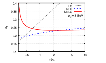
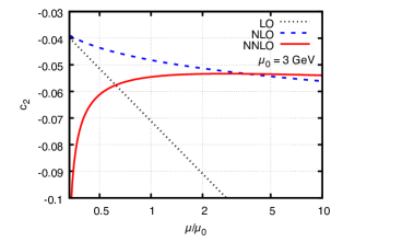
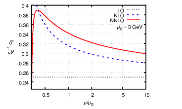
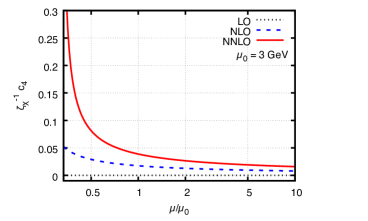
Figure 1: Renormalization-scale dependence of the coefficients $c_{1}$, $c_{2}$, $\mathring{c}_{3}=\zeta^{-1}_{\chi}c_{3}$, $\mathring{c}_{4}=\zeta^{-1}_{\chi}c_{4}$, defined in Eqs. (46)–(49), with $\zeta_{\chi}$ from Eq. (52). The dotted black, dashed blue, and solid red curve correspond to keeping terms up to order $(g^{2})^{n-1}$ in $c_{1}$ and $c_{2}$, and $(g^{2})^{n}$ in $\mathring{c}_{3}$ and $\mathring{c}_{4}$, with $n=0,1,2$, respectively. The central scale is set to $\mu_{0}=3$ GeV, corresponding to $t=3.12\cdot 10^{-2}/\text{GeV}^{2}$, see Eq. (55). The number of flavors is set to $n_{F}=3$.

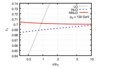
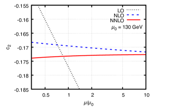
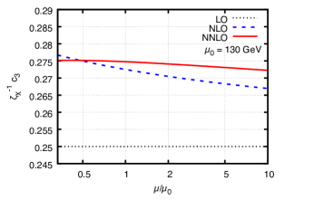
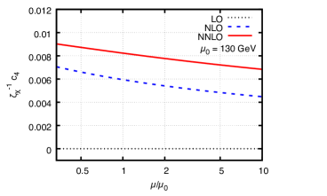
Figure 2: Same as Fig. 1, but for $\mu_{0}=130$ GeV (or $t=1.66\cdot 10^{-5}/\text{GeV}^{2}$), and $n_{F}=5$.

As opposed to the gluonic coefficients $c_{1}$ and $c_{2}$, the coefficients of the fermionic operators $c_{3}$ and $c_{4}$ exhibit a residual scale dependence only from the NLO term onwards. One therefore expects a stronger $\mu$-dependence at NNLO for these terms. Nevertheless, for $\mathring{c}_{3}$, the estimate of the theory uncertainty due to scale variation still decreases from $9.8$% to $8.1$%. The increase of the result due to the NNLO effects is $8.3$% relative to the NLO result at $\mu=\mu_{0}$.

The behavior of $\mathring{c}_{4}$, on the other hand, is less satisfactory at $\mu_{0}=3$ GeV. The NNLO effects more than double the NLO result in this case, and the uncertainty estimate due to scale variation actually increases from 47% to 71% when going from NLO to NNLO. Note, however, that $c_{4}=0$ at LO, which means that this coefficient is numerically sub-dominant.

As one would expect, for $\mu_{0}=130$ GeV, the perturbative behavior of all coefficients is significantly improved, cf. Fig. 2. For $c_{1}$, $c_{2}$, and $\mathring{c}_{3}$, the scale uncertainty is at the sub-percent level already at NLO; at NNLO, it amounts to less than $0.2$% in all three cases. The effect of the NNLO corrections relative to the NLO result is about $2$% for $c_{1}$ and $c_{2}$, and $0.8$% for $\mathring{c}_{3}$. Also for $\mathring{c}_{4}$, the situation improves significantly: the NNLO terms add 38% to the NLO result, and the uncertainty goes down from 10% at NLO to $5.8$% at NNLO.

It is also worth pointing out that the choice of the central scale $\mu_{0}$ as defined in Eq. (55) seems justified by the behavior of the successively higher orders. In almost all cases, the NLO and the NNLO corrections are both relatively small at $\mu=\mu_{0}$. At the same time, the NNLO corrections relative to the NLO result are always smaller than the NLO corrections compared to the LO result. The only exception to this is $\mathring{c}_{4}$ at $\mu_{0}=3$ GeV, where, however, no choice of $\mu$ seems to stand out over any other.

In summary, we conclude that the NNLO terms lead to a significant improvement of the perturbative accuracy of the Wilson coefficients.

6 Trace anomaly

As a test of our result, we use the trace anomaly of the EMT. As suggested in Ref. [Nielsen:1977sy], a simple derivation consists of taking the trace of the EMT in $D=4-2\epsilon$ dimensions. By use of the equations of motion, this gives for the gauge invariant part

$$T_{\mu\mu}=\frac{\epsilon}{2g_{0}^{2}}F_{\rho\sigma}^{a}F_{\rho\sigma}^{a}-\sum_{f=1}^{n_{F}}m_{f,0}\overline{\psi}_{f}\psi_{f}=\frac{1}{2D}\left(\frac{\epsilon}{g_{0}^{2}}\mathcal{O}_{2,\mu\mu}+\mathcal{O}_{4,\mu\mu}\right)\,,$$ (56)

where we have used Eq. (10) in the last step. Using the mixing matrix $\zeta_{ij}(t)$, we can rewrite this in terms of flowed operators:

$$\begin{split}T_{\mu\mu}=\bar{c}_{i}(t)\tilde{\mathcal{O}}_{i,\mu\mu}(t,x)\,,\qquad\bar{c}_{i}(t)=\frac{1}{2D}\left(\frac{\epsilon}{g_{0}^{2}}\zeta_{2i}^{-1}(t)+\zeta_{4i}^{-1}(t)\right)\,.\end{split}$$ (57)

Note that $\bar{c}_{1}(t)=\bar{c}_{3}(t)=0$, as $\tilde{\mathcal{O}}_{1,\mu\nu}(t,x)$ and $\tilde{\mathcal{O}}_{3,\mu\nu}(t,x)$ have a non-trivial index structure and therefore $\mathcal{O}_{2,\mu\nu}(x)$ and $\mathcal{O}_{4,\mu\nu}(x)$ cannot mix with them. Since $\tilde{\mathcal{O}}_{2,\mu\mu}=D\tilde{\mathcal{O}}_{1,\mu\mu}$ and $2\tilde{\mathcal{O}}_{4,\mu\mu}=D\tilde{\mathcal{O}}_{3,\mu\mu}$, we cannot equate coefficients with Eq. (15) for all $i$ individually. Instead, only the weaker conditions

$$\begin{split}c_{1}(t)+Dc_{2}(t)=D\bar{c}_{2}(t)\,,\qquad 2c_{3}(t)+Dc_{4}(t)=D\bar{c}_{4}(t)\,.\end{split}$$ (58)

can be derived. We checked that these equations are indeed fulfilled by our result.

7 Operator renormalization

Using the fact that flowed operators are finite after mass and field renormalization, we can also compute the renormalization matrix for the regular QCD operators $\{\mathcal{O}_{1,\mu\nu}(x),$ $\mathcal{O}_{2,\mu\nu}(x),\mathcal{O}_{3,\mu\nu}(x),\mathcal{O}_{4,\mu\nu}(x)\}$ defined in Eq. (8). It is convenient to define an equivalent set of operators as

$$\begin{split}&\hat{\mathcal{O}}_{i,\mu\nu}(x)=H_{ij}\mathcal{O}_{j,\mu\nu}(x)\,,\qquad\mbox{where}\quad H_{ij}=\left\{\begin{array}[]{l}1/g_{0}^{2}\quad\text{for}\ i=j\in\{1,2\}\,,\\ 1\quad\text{for}\ i=j\in\{3,4\}\,,\\ 0\quad\text{for}\ i\neq j\end{array}\right.\,.\end{split}$$ (59)

This multiplication of $\mathcal{O}_{1,\mu\nu}$ and $\mathcal{O}_{2,\mu\nu}$ by $1/g_{0}^{2}$ ensures that the mass dimension of all operators $\hat{\mathcal{O}}_{i,\mu\nu}$ is equal to $D$. The renormalization matrix is then defined as

$$\{\hat{\mathcal{O}}_{i}\}_{R}(x)=Z_{ij}\hat{\mathcal{O}}_{j}(x)\,.$$ (60)

Expressing the $\hat{\mathcal{O}}_{i,\mu\nu}(x)$ in terms of flowed operators, one can determine its entries in the $\overline{\mbox{{MS}}}$ scheme by demanding that

$$\{\hat{\mathcal{O}}_{i}\}_{R}(x)=Z_{ij}\,H_{jk}\,\zeta_{kl}^{-1}(t)\,\tilde{\mathcal{O}}_{l}(t,x)$$ (61)

be finite. In analogy to Eqs. (41) and (44), we write

$$Z_{ij}=\delta_{ij}-\frac{g^{2}}{(4\pi)^{2}}\frac{\gamma_{0,ij}}{2\epsilon}+\frac{g^{4}}{(4\pi)^{4}}\left[\frac{1}{\epsilon^{2}}\left(\frac{\gamma_{0,ik}\gamma_{0,kj}}{8}+\frac{\beta_{0}}{4}\gamma_{0,ij}\right)-\frac{\gamma_{1,ij}}{4\epsilon}\right]+{\cal O}(g^{6})\,.$$ (62)

Our result for the coefficients of the anomalous dimension at NLO is in agreement with Ref. [Makino:2014taa]:

$$\gamma_{0}=\begin{pmatrix}-\frac{8}{3}T_{F}&\frac{11}{6}C_{A}&\frac{4}{3}C_{F}&\frac{7}{3}C_{F}\\ 0&\frac{22}{3}C_{A}-\frac{8}{3}T_{F}&0&12C_{F}\\ \frac{32}{3}T_{F}&-\frac{8}{3}T_{F}&-\frac{16}{3}C_{F}&\frac{8}{3}C_{F}\\ 0&0&0&0\end{pmatrix}\,.$$ (63)

At NNLO, we find

$$\gamma_{1,11} =-\frac{140}{27}C_{A}T_{F}-\frac{296}{27}C_{F}T_{F}\,, \gamma_{1,12} =\frac{34}{3}C_{A}^{2}-\frac{112}{27}C_{A}T_{F}-\frac{10}{27}C_{F}T_{F}\,,$$ (64)

$$\gamma_{1,13} =\frac{188}{27}C_{A}C_{F}-\frac{56}{27}C_{F}^{2}-\frac{104}{27}C_{F}T_{F}\,, \gamma_{1,14} =\frac{812}{27}C_{A}C_{F}+\frac{85}{27}C_{F}^{2}-\frac{44}{27}C_{F}T_{F}\,,$$

$$\gamma_{1,21} =0\,, \gamma_{1,22} =\frac{136}{3}C_{A}^{2}-\frac{80}{3}C_{A}T_{F}-16C_{F}T_{F}\,,$$

$$\gamma_{1,23} =0\,, \gamma_{1,24} =\frac{388}{3}C_{A}C_{F}+12C_{F}^{2}-\frac{80}{3}C_{F}T_{F}\,,$$

$$\gamma_{1,31} =\frac{560}{27}C_{A}T_{F}+\frac{1184}{27}C_{F}T_{F}\,, \gamma_{1,32} =-\frac{272}{27}C_{A}T_{F}-\frac{392}{27}C_{F}T_{F}\,,$$

$$\gamma_{1,33} =-\frac{752}{27}C_{A}C_{F}+\frac{224}{27}C_{F}^{2}+\frac{416}{27}C_{F}T_{F}\,, \gamma_{1,34} =\frac{244}{27}C_{A}C_{F}-\frac{16}{27}C_{F}^{2}-\frac{544}{27}C_{F}T_{F}\,,$$

$$\gamma_{1,41} =\gamma_{1,42}=\gamma_{1,43}=\gamma_{1,44}=0\,.$$

The renormalization matrix $Z_{ij}$ and the mixing matrix $\zeta_{ij}$ are provided in ancillary files with this paper. In this way, one obtains the following expression for the energy-density operator in terms of flowed operators, for example:

$$\begin{split}\bigg{\{}\frac{1}{g_{0}^{2}}&F_{\mu\nu}(x)F_{\mu\nu}(x)\bigg{\}}_{R}=\frac{Z_{2j}H_{jk}}{D}\left[\zeta_{k2}^{-1}(t)\,\tilde{\mathcal{O}}_{2,\mu\mu}(t,x)+\zeta_{k4}^{-1}(t)\tilde{\mathcal{O}}_{4,\mu\mu}(t,x)\right]\\ &=\frac{1}{g^{2}}G_{\mu\nu}(t,x)G_{\mu\nu}(t,x)\Bigg{\{}1-\frac{7}{2}C_{A}\frac{g^{2}}{(4\pi)^{2}}\\ &\qquad+\frac{g^{4}}{(4\pi)^{4}}\Bigg{[}\left(-\frac{3}{2}\,C_{A}^{2}-2\,C_{A}T_{F}-14\,C_{F}T_{F}\right)L(\mu,t)\\ &\qquad\quad+C_{A}^{2}\left(-\frac{1427}{180}+\frac{87}{5}\ln 2-\frac{54}{5}\ln 3\right)+\frac{8}{9}\,C_{A}T_{F}-\frac{34}{3}\,C_{F}T_{F}\Bigg{]}\Bigg{\}}\\ &\quad+Z_{\chi}\sum_{f=1}^{n_{F}}\bar{\chi}_{f}(t,x)\overleftrightarrow{\not{\mathcal{D}}}\chi_{f}(t,x)\Bigg{\{}\frac{g^{2}}{(4\pi)^{2}}C_{F}\left(5+6L(\mu,t)\right)\\ &\qquad+\frac{g^{4}}{(4\pi)^{4}}\Bigg{[}\gamma_{\chi,0}\left(\beta_{0}+\frac{\gamma_{\chi,0}}{2}\right)L^{2}(\mu,t)\\ &\qquad\quad+\left(\frac{304}{3}\,C_{A}C_{F}+18\,C_{F}^{2}-\frac{80}{3}\,C_{F}T_{F}\right)L(\mu,t)\\ &\qquad\quad+C_{A}C_{F}\left(-2\text{Li}_{2}\left(\frac{1}{4}\right)+\frac{2923}{30}-\frac{4}{3}\pi^{2}+\frac{8546}{15}\ln 2-\frac{2139}{5}\ln 3\right)\\ &\qquad\quad+6\,C_{F}^{2}-C_{F}T_{F}\left(30+\frac{4}{3}\pi^{2}\right)\Bigg{]}\Bigg{\}}\,.\end{split}$$ (65)

Through NLO, this result agrees with Refs. [Makino:2014taa, Suzuki:2018vfs]. Similar relations can be derived for all other operators of Eq. (8), of course.

8 Conclusions

We have presented the universal Wilson coefficients for the gradient-flow definition of the energy-momentum tensor through NNLO QCD. The NNLO corrections modify the three numerically dominant coefficients $c_{1}$, $c_{2}$, $\mathring{c}_{3}$ at the level of 10% (1-2%) for a central scale of $\mu_{0}=3$ GeV ($\mu_{0}=130$ GeV), where $\mu_{0}$ is related to the flow time $t$ according to Eq. (55). We observe a reduction of the theoretical uncertainty relative to the NLO result as derived from varying the renormalization scale by a factor of two around its central value. The behavior of the fourth coefficient $\mathring{c}_{4}$ is less satisfactory, but its impact is expected to be numerically suppressed.

Aside from this main outcome, new results presented in this paper include the flowed quark-field renormalization constant to NNLO in the $\overline{\mbox{{MS}}}$ scheme, and the anomalous dimension matrix for the regular QCD operators which make up the EMT.

In conclusion, we hope that our results will help to improve the studies of the EMT on the lattice. They are the first outcome of a systematic setup for higher-order perturbative calculations within the gradient-flow formalism [Artz:2019bpr], which should prove useful also in other applications of this theoretical framework.

Acknowledgments.

We are indebted to Johannes Artz and Mario Prausa for helping to establish the setup within which this calculation was performed. We would also like to thank Tobias Neumann for fruitful communication, and for providing his tools which enabled us to obtain $\mathring{Z}_{\chi}$ before the publication of Ref. [Artz:2019bpr]. Further thanks go to Mauro Papinutto for pointing out a typo in an earlier version of this manuscript. This work was supported by Deutsche Forschungsgemeinschaft (DFG), project 386986591.

Appendix A Feynman rules

In this section, we present the Feynman rules for the operators defined in Eq. (8) in regular QCD. Only the terms which are relevant for the construction of the projectors in Eqs. (22) and (24) are listed explicitly. All momenta are understood to be outgoing.

$$\mathcal{O}_{1,\mu\nu} =\partial_{\mu}A_{\rho}^{c}\partial_{\nu}A_{\rho}^{c}+\cdots \Rightarrow \begin{gathered}\includegraphics{dias/O1.pdf}\end{gathered}= -p_{1,\mu}p_{2,\nu}\delta_{\alpha\beta}\delta^{ab}$$ (67)

$$\mathcal{O}_{2,\mu\nu} =2\delta_{\mu\nu}\partial_{\rho}A_{\sigma}^{c}\partial_{\rho}A_{\sigma}^{c}+\cdots \Rightarrow \begin{gathered}\includegraphics{dias/O1.pdf}\end{gathered}= -4\delta_{\mu\nu}p_{1}\cdot p_{2}\delta_{\alpha\beta}\delta^{ab}$$ (69)

$$\mathcal{O}_{3f,\mu\nu} =\bar{\psi}_{f}\gamma_{\mu}\partial_{\nu}\psi_{f}+\cdots \Rightarrow \begin{gathered}\includegraphics{dias/O3.pdf}\end{gathered}= \,i\gamma_{\mu}p_{2\nu}\delta^{ij}$$ (71)

$$\mathcal{O}_{4f,\mu\nu} =\delta_{\mu\nu}\bar{\psi}_{f}\not{\partial}\psi_{f}+\cdots \Rightarrow \begin{gathered}\includegraphics{dias/O3.pdf}\end{gathered}= \,i\delta_{\mu\nu}\not{p}_{2}\delta^{ij}$$ (73)

$$\mathcal{O}_{5f,\mu\nu} =\delta_{\mu\nu}m_{0}\bar{\psi}_{f}\psi_{f} \Rightarrow \begin{gathered}\includegraphics{dias/O3.pdf}\end{gathered}= \,\delta_{\mu\nu}m_{0}\delta^{ij}$$ (75)

References

- [1] M. Lüscher, Properties and uses of the Wilson flow in lattice QCD, JHEP 1008, 071 (2010)