Distribution of Energy-Momentum Tensor around a Static Quark
in the Deconfined Phase of SU(3) Yang-Mills Theory

Abstract

Energy momentum tensor (EMT) characterizes the response of the vacuum as well as the thermal medium under the color electromagnetic fields. We define the EMT by means of the gradient flow formalism and study its spatial distribution around a static quark in the deconfined phase of SU(3) Yang-Mills theory on the lattice. Although no significant difference can be seen between the EMT distributions in the radial and transverse directions except for the sign, the temporal component is substantially different from the spatial ones near the critical temperature $T_{c}$. This is in contrast to the prediction of the leading-order thermal perturbation theory. The lattice data of the EMT distribution also indicate the thermal screening at long distance and the perturbative behavior at short distance.

I Introduction

To study complex quantum systems such as the Yang-Mills (YM) theory, it is customary to introduce test probe(s) and analyze the response. The Wilson loop is one of such probes whose measurement in YM theory provides information on the static quark–anti-quark system that is closely related to the confinement property in YM vacuum Bali:2000gf . Thanks to the recent development of the gradient-flow method Narayanan:2006rf ; Luscher:2010iy ; Luscher:2011bx and its application to the energy-momentum tensor (EMT) $\mathcal{T}_{\mu\nu}(x)$ Suzuki:2013gza ; Makino:2014taa ; Hieda:2016xpq ; Harlander:2018zpi , it became possible to study the gauge-invariant structure of the flux tube between the quark and anti-quark in the confining phase through the spatial distribution of EMT under the Wilson loop Yanagihara:2018qqg ; Yanagihara:2019foh .

The purpose of the present paper is to extend the above idea and to explore the EMT distribution around a static quark in YM theory. As a first step, we consider the deconfined phase above the critical temperature $T_{c}$ of the SU(3) YM theory in the range of temperature $1.2\leq T/T_{c}\leq 2.6$ and measure the EMT distribution around the Polyakov loop. The EMT with the gradient flow has been used to study thermodynamics of YM theory Asakawa:2013laa ; Kitazawa:2016dsl ; Kitazawa:2017qab ; Iritani:2018idk ; Hirakida:2018uoy ; Kitazawa:2019otp and of QCD Taniguchi:2016ofw ; Taniguchi:2020mgg . However, the observables in these studies are limited to global quantities such as the pressure, energy density, entropy density, and the specific heat. On the other hand, we focus on the local observable in this study and examine the following questions: (i) How are the energy density and the stress tensor distributed around the static quark?, (ii) How are the distributions modified as a function of temperature?, and (iii) How can one extract parameters such as the running coupling and the Debye screening mass from the distributions?

The organization of the present paper is as follows. In Sec. II, we briefly review the definition of EMT and its property in the spherical coordinate system. In Sec. III, we introduce the EMT operator on the lattice and its correlation with the Polyakov loop operator. In Sec. IV, we discuss the numerical procedure and lattice setup to analyze the EMT operator around a static quark on the lattice. Numerical results and their physical implications are given in Sec. V. Sec. VI is devoted to the summary and conclusion. In Appendix A, we discuss the procedure to make the tree-level improvement of the correlation between the EMT and the Polyakov loop on the lattice. In Appendix B, the leading-order perturbative analysis of the correlation is presented using the high temperature effective field theory.

II EMT around a static charge

The stress tensor $\sigma_{ij}\,(i,j=1,2,3)$ is related to the spatial component of EMT, $\mathcal{T}_{ij}$, as Landau

$$\sigma_{ij}=-\mathcal{T}_{ij}.$$ (1)

The force per unit area ${\cal F}_{i}$ acting on a surface with the normal vector $n_{i}$ is given by the stress tensor as

$${\cal F}_{i}=\sigma_{ij}n_{j}=-{\cal T}_{ij}n_{j}.$$ (2)

The local principal axes $n_{j}^{(k)}$ and the corresponding eigenvalues $\lambda_{k}$ of the local stress tensor are obtained by solving the eigenvalue problem:

$${\cal T}_{ij}n_{j}^{(k)}=\lambda_{k}n_{i}^{(k)}\quad(k=1,2,3).$$ (3)

The strength of the force per unit area along $n_{i}^{(k)}$ is given by the absolute values of the eigenvalue $\lambda_{k}$. Neighboring volume elements separated by a surface with the normal vector $n_{i}^{(k)}$ pull (push) each other for $\lambda_{k}<0$ ($\lambda_{k}>0$) across the wall. Note that the three principal axes $n_{i}^{(k)}$ are orthogonal with one another because $\sigma_{ij}$ is a symmetric tensor.

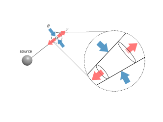
Figure 1: Stress acting on infinitely small volume element under the existence of a single static charge (source). In the case of the classical electromagnetism, a small volume element at a distance of $r$ from the charge is pulled along the radial direction from the neighboring volume elements while it is pushed in the transverse direction.

For a system with a single static source, it is convenient to use the spherical coordinate system $(r,\theta,\varphi)$ with the radial coordinate $r=|\bm{x}|$, and the polar and azimuthal angles $\theta$ and $\varphi$. The spherical symmetry allows us to diagonalize the static EMT in Euclidean spacetime $\mathcal{T}_{\mu\nu}(\bm{x})$ in this coordinate system as

$$\mathcal{T}_{\gamma\gamma^{\prime}}(\bm{x}) =\mathrm{diag}(\mathcal{T}_{44}(r),\mathcal{T}_{rr}(r),\mathcal{T}_{{\theta\theta}}(r))$$ (4)

where $\gamma,\gamma^{\prime}={4,r,\theta}$. Due to the spherical symmetry, the azimuthal component degenerates with the polar component, $\mathcal{T}_{\varphi\varphi}(r)=\mathcal{T}_{\theta\theta}(r)$, so that only independent components are given in Eq. (4).

In the Abelian case, EMT is given by the Maxwell stress-energy tensor Landau , $\mathcal{T}^{\mathrm{Maxwell}}_{\mu\nu}={F}_{\mu\rho}{F}_{\nu\rho}-\frac{1}{4}\delta_{\mu\nu}{F}_{\rho\sigma}{F}_{\rho\sigma}$ with the field strength ${F}_{\mu\nu}$. When a static charge is placed at the origin, the EMT is denoted by

$$\mathcal{T}_{\gamma\gamma^{\prime}}^{\rm Maxwell}=\frac{1}{2}\mathrm{diag}(-\vec{E}^{2},-\vec{E}^{2},\vec{E}^{2}),$$ (5)

with ${E}_{i}(\bm{x})$ being the electric field. The spatial structure of Eq. (5) is illustrated in Fig. 1 where the neighboring volume elements around the static electric charge pull (push) each other along the radial (angular) direction. In a static system, the force acting on a volume element through its surface should be balanced. This property is guaranteed by the momentum conservation $\partial_{i}\mathcal{T}_{ij}=0$ together with the Gauss theorem.

III EMT for SU(3) Yang-Mills theory on the lattice

III.1 YM gradient flow

We consider the pure SU(3) YM gauge theory in the four-dimensional Euclidean space defined by the action,

$$S_{\mathrm{YM}}=\frac{1}{4g_{0}^{2}}\int d^{4}x\,G_{\mu\nu}^{a}(x)G_{\mu\nu}^{a}(x).$$ (6)

Here $g_{0}$ is a bare gauge coupling and $G_{\mu\nu}^{a}(x)$ is the field strength composed of the fundamental gauge field $A_{\mu}^{a}(x)$. The YM gradient flow evolves the gauge field along the fictitious fifth dimension $t$ introduced in addition to the ordinary four Euclidean dimensions $x$ through the flow equation  Narayanan:2006rf ; Luscher:2010iy ; Luscher:2011bx ,

$$\frac{dA_{\mu}^{a}(t,x)}{dt}=-g_{0}^{2}\frac{\delta S_{\mathrm{YM}}(t)}{\delta A_{\mu}^{a}(t,x)}.$$ (7)

The flowed YM action $S_{\mathrm{YM}}(t)$ in the $(4+1)$-dimensional coordinate is constructed by substituting the flowed gauge field $A_{\mu}^{a}(t,x)$ in Eq. (6) with an initial condition, $A_{\mu}^{a}(t=0,x)=A_{\mu}^{a}(x)$.

An important feature of the gradient flow for $t>0$ is that any composite operators composed of flowed gauge fields are UV finite even at equal spacetime point Luscher:2011bx ; Hieda:2016xpq . This is a consequence of the smoothing of the gauge fields in the four dimensional Euclidean space within the range $\sim\sqrt{2t}$. In addition, in the small $t$ limit, composite local operators are represented by the local operators of the ordinary gauge theory at $t=0$. These properties lead us to the renormalized EMT operator defined with the small $t$ expansion Suzuki:2013gza :

$${\cal T}_{\mu\nu}^{\rm R}(x) = \lim_{t\to 0}{\cal T}_{\mu\nu}(t,x),$$ (8)

$${\cal T}_{\mu\nu}(t,x) = c_{1}(t)U_{\mu\nu}(t,x)$$ (9)

$$+4c_{2}(t)\delta_{\mu\nu}\left[E(t,x)-\left\langle E(t,x)\right\rangle_{0}\right],$$

where $\langle E(t,x)\rangle_{0}$ is the vacuum expectation value of $E(t,x)$. The dimension-four gauge-invariant operators on the right hand side of Eq. (9) are given by Suzuki:2013gza

$$E(t,x) =\frac{1}{4}G_{\mu\nu}^{a}(t,x)G_{\mu\nu}^{a}(t,x),$$ (10)

$$U_{\mu\nu}(t,x) =G_{\mu\rho}^{a}(t,x)G_{\nu\rho}^{a}(t,x)-\delta_{\mu\nu}E(t,x),$$ (11)

where $G_{\mu\nu}^{a}(t,x)$ is the field strength composed of the flowed gauge field. Because of the vacuum subtraction in Eq. (9), $\langle{\cal T}_{\mu\nu}^{\rm R}(x)\rangle_{0}$ vanishes. The coefficients $c_{1}(t)$ and $c_{2}(t)$ have been calculated perturbatively in Refs. Suzuki:2013gza ; Harlander:2018zpi ; Iritani:2018idk for small $t$. We use two-loop perturbative coefficients Harlander:2018zpi ; Iritani:2018idk for the construction of EMT throughout this study.

III.2 EMT around a static heavy quark

To describe a static quark $Q$ on the lattice, we introduce the Polyakov loop at the origin, $\Omega(\bm{0})$. Then the expectation value of Eq. (9) around $Q$ is given by

$$\langle\mathcal{T}_{\mu\nu}(t,x)\rangle_{Q}=\frac{\langle\mathcal{T}_{\mu\nu}(t,x)\mathrm{Tr}\Omega(\bm{0})\rangle}{\langle\mathrm{Tr}\Omega(\bm{0})\rangle}-\langle\mathcal{T}_{\mu\nu}(t,x)\rangle.$$ (12)

We note that Eq. (12) is well-defined only when the $Z_{3}$ symmetry in SU(3) YM theory is spontaneously broken: In the $Z_{3}$ unbroken phase, both numerator and denominator of the first term on the right hand side vanish exactly. This is the reason why we focus on the system in the $Z_{3}$ broken phase above $T_{c}$ in this paper. In practice, we choose the state with the Polyakov loop being real among the three equivalent $Z_{3}$ states in the deconfined phase.

The renormalized EMT distribution around $Q$ is obtained after taking the double extrapolation,

$$\langle\mathcal{T}^{\mathrm{R}}_{\mu\nu}(x)\rangle_{Q}=\lim_{t\rightarrow 0}\lim_{a\rightarrow 0}\langle\mathcal{T}_{\mu\nu}(t,x)\rangle_{Q}.$$ (13)

In our actual analysis, we extract the renormalized EMT distribution by fitting the lattice data with the following functional form Kitazawa:2016dsl ; Kitazawa:2017qab :

$$\langle\mathcal{T}_{\mu\nu}(t,x)\rangle_{Q}=\langle\mathcal{T}^{\mathrm{R}}_{\mu\nu}(x)\rangle_{Q}+b_{\mu\nu}{(t)}a^{2}+c_{\mu\nu}t+d_{\mu\nu}t^{2},$$ (14)

where the contributions from discretization effects ($b_{\mu\nu}$) as well as the dimension-six and -eight operators ($c_{\mu\nu}$ and $d_{\mu\nu}$) are considered.

To perform the double extrapolation reliably, the smearing radius $\rho\equiv\sqrt{2t}$ needs to be larger than the lattice spacing to suppress the discretization error. At the same time, $\rho$ should be smaller than half the temporal size $1/2T$ with temperature $T$ as well as the distance from the source ($r$) to avoid the overlap of operators. Therefore we require

$$a/2\lesssim\rho\lesssim\mathrm{min}\Bigl{(}r,\frac{1}{2T}\Bigr{)}.$$ (15)

The lattice data to be fitted by Eq. (14) should be within this window. As will be discussed in Sec. IV.3, we impose more stringent conditions for the range of $t$ in our numerical analysis.

IV Lattice setup

IV.1 Gauge configurations

Numerical simulations in SU(3) YM theory were performed on the four dimensional Euclidean lattice with the Wilson gauge action and the periodic boundary conditions at four different temperatures $1.20T_{c},\,1.44T_{c},\,2.00T_{c}$, and $2.60T_{c}$. The simulation parameters for each $T$ are summarized in Table 1. The inverse coupling $\beta=6/g_{0}^{2}$ is related to the lattice spacing $a$ determined by the reference scale $w_{0}$ Kitazawa:2016dsl ; Borsanyi:2012zs . The spatial and temporal lattice sizes, $N_{s}$ and $N_{\tau}$ together with the number of configurations $N_{\mathrm{conf}}$ are also summarized in Table 1. All lattices have the same aspect ratio $N_{s}/N_{\tau}=4$.

Table 1: Simulation parameters for the four temperatures: The spatial lattice size $N_{s}$, the temporal lattice size $N_{\tau}$, $\beta=6/g_{0}^{2}$, the lattice spacing $a$. $N_{\mathrm{conf}}$ represents the number of configurations.

$T/T_{c}$	$N_{s}$	$N_{\tau}$	$\beta$	$a~{}[\mathrm{fm}]$	$N_{\mathrm{conf}}$
1.20	40	10	6.336	0.0551	500
	48	12	6.467	0.0460	650
	56	14	6.581	0.0394	840
	64	16	6.682	0.0344	1,000
	72	18	6.771	0.0306	1,000
1.44	40	10	6.465	0.0461	500
	48	12	6.600	0.0384	650
	56	14	6.716	0.0329	840
	64	16	6.819	0.0288	1,000
	72	18	6.910	0.0256	1,000
2.00	40	10	6.712	0.0331	500
	48	12	6.853	0.0275	650
	56	14	6.973	0.0236	840
	64	16	7.079	0.0207	1,000
	72	18	7.173	0.0184	1,000
2.60	40	10	6.914	0.0255	500
	48	12	7.058	0.0212	650
	56	14	7.182	0.0182	840
	64	16	7.290	0.0159	1,000
	72	18	7.387	0.0141	1,000

The gauge configurations are generated by the pseudo-heat-bath method followed by five over-relaxations. Each measurement is separated by 200 sweeps. Statistical errors are estimated by the jackknife method with 20 jackknife bins. We employ the Wilson gauge action for $S_{\mathrm{YM}}(t)$ in the flow equation Eq. (7) and the clover type representation for the field strength $G_{\mu\nu}(t,x)$. The numerical solution of the gradient flow equation is obtained by the third order Runge-Kutta method.

In order to suppress the statistical noise, we apply the multi-hit procedure in the measurement of the Polyakov loop by replacing every temporal link by its thermal average Parisi:1983hm . The choice of the temporal argument $x_{4}$ of EMT in Eq. (12) is arbitrary. Therefore, we average EMT over the temporal direction to reduce the statistical error.

IV.2 Discretization effect

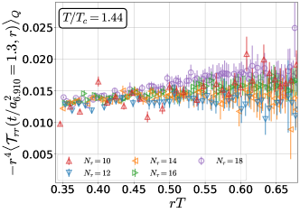
Figure 2: Distribution of $-r^{4}\langle\mathcal{T}_{rr}(t/a_{6.910}^{2}=1.3,r)\rangle_{Q}$ as functions of $rT$ at $T/T_{c}=1.44$.

The EMT in the spherical coordinate system on the lattice reads

$$T\sum_{x_{4}}\langle\mathcal{T}_{\gamma\gamma^{\prime}}(t,\bm{x},x_{4})\rangle_{Q}$$

$$=\mathrm{diag}(\langle\mathcal{T}_{44}(t,r)\rangle_{Q},\langle\mathcal{T}_{rr}(t,r)\rangle_{Q},\langle\mathcal{T}_{\theta\theta}(t,r)\rangle_{Q}).$$ (16)

The behavior of the EMT distribution close to the source $Q$ is affected by the violation of rotational symmetry owing to lattice discretization. As an example, we show in Fig. 2 the distribution of $-r^{4}\langle\mathcal{T}_{rr}(t/a_{6.910}^{2}=1.3,r)\rangle_{Q}$ as a function of $rT$ at $T/T_{c}=1.44$, where $a_{6.910}$ is the lattice spacing of the finest lattice at this temperature. The figure shows the oscillating behavior of the numerical results becomes more prominent on coarser lattices. In this study, we use the lattice data only for $N_{\tau}\geq 12$ for the continuum extrapolation to suppress the discretization errors. In Appendix A, we consider an alternative analysis that performs the tree-level improvement of the numerical results and uses them for the continuum extrapolation with the $N_{\tau}=10$ data. As discussed there, we confirm that the results in both cases are the same within the errors.

IV.3 Double extrapolation

The double extrapolation Eq. (13) consists of two steps: (I) the continuum ($a\to 0$) extrapolation, and (II) $t\to 0$ extrapolation. In this subsection, we demonstrate these procedures by using the lattice data at $T/T_{c}=1.44$ as an example.

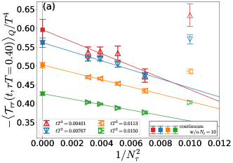
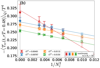
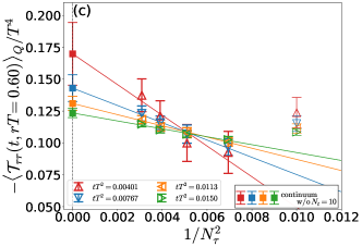
Figure 3: Color open symbols represent $-\langle\mathcal{T}_{rr}(t,rT)\rangle_{Q}/T^{4}$ for various $t$ as functions of $1/N_{\tau}^{2}=a^{2}T^{2}$ at $T/T_{c}=1.44$. The continuum extrapolation for each $t$ is shown by the solid lines, with the extrapolated results represented by the filled symbols. Panels (a), (b) and (c) show the results at $rT=0.40,0.48,0.60$, respectively.

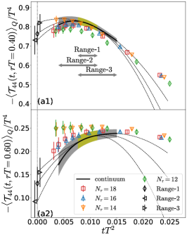
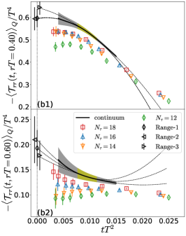
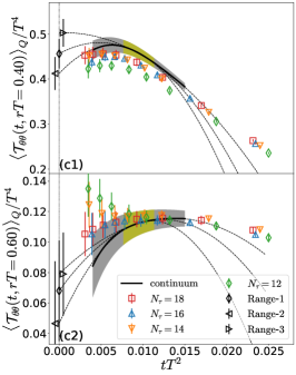
Figure 4: Each component of EMT at $rT=0.40$ (top) and $rT=0.60$ (bottom) as functions of $tT^{2}$. Color open symbols denote $\langle\mathcal{T}_{\gamma\gamma^{\prime}}(t,rT)\rangle_{Q}/T^{4}$ for each $a$ as functions of $tT^{2}$. The black solid line with the gray error band is the continuum-extrapolated result. The dotted lines show the fitted results of the continuum result with Range-1, 2, and 3. The black symbols are the results of the $t\to 0$ extrapolation for these fitting ranges.

In Fig. 3, we show $-\langle\mathcal{T}_{rr}(t,rT)\rangle_{Q}/T^{4}$ at $rT=0.40,0.48,0.60$ as a function of $1/N_{\tau}^{2}=(aT)^{2}$ for four values of $tT^{2}$. To obtain the EMT values at a given $r$ and $t$, we first perform the linear interpolation of the lattice data along the $r$ direction and then interpolate along the $t$ direction by the cubic spline method for each $a$.

In Fig. 3, fitting results of the data at $N_{\tau}=12$–$18$ according to Eq. (14) at fixed $t$ are shown by the solid lines, while the results of the continuum limit are shown by the filled squares on the vertical dotted line at $1/N_{\tau}^{2}=0$. We then take $t\rightarrow 0$ extrapolation by fitting the continuum-extrapolated results for different $t$ with Eq. (14) at $a=0$. This fit has to be carried out within the range of $t$ satisfying Eq. (15). We employ $tT^{2}=0.00401$ corresponding to $t/a^{2}=1.3$ of the finest lattice data as the lower bound of the fitting window: This choice satisfies Eq. (15) for all the lattices. The upper bound of the fitting window is taken to be $tT^{2}=0.015$, since the thermodynamic quantities show a linear behavior below this value  Kitazawa:2016dsl .

We consider the following three ranges within $0.00401\leq tT^{2}\leq 0.015$ to estimate the systematic uncertainty from the fitting ranges Kitazawa:2016dsl :

$$\mathrm{Range\mathchar 45\relax 1}:0.00767\leq tT^{2}\leq 0.0113,$$

$$\mathrm{Range\mathchar 45\relax 2}:0.00401\leq tT^{2}\leq 0.0113,$$

$$\mathrm{Range\mathchar 45\relax 3}:0.00767\leq tT^{2}\leq 0.0150.$$

Range-1 is the most conservative window, while Range-2 (Range-3) is the extension of Range-1 towards the smaller (larger) values of $t$. We employ the result of Range-1 as a central value and use the Range-2 and Range-3 for an estimate of the systematic error. In the following, all the results after the double extrapolation contain both the statistical and systematic errors.

In Fig. 4, the open symbols with statistical errors represent $\langle\mathcal{T}_{\gamma\gamma^{\prime}}(t,rT)\rangle_{Q}/T^{4}$ at $rT=0.40$ (upper) and $0.60$ (lower) for each $a$. The results of the continuum limit are denoted by the black solid lines with the gray statistical error band for $0.00401\leq tT^{2}\leq 0.015$. Range-1 is highlighted by the yellow band. The figure also shows the fitted results for Ranges-1, 2, and 3 by the dotted lines. The final results of the $t\to 0$ limit for each range are shown by the open black symbols around $tT^{2}=0$: They agree with each other within the statistical errors, which suggests that the systematic uncertainty from the choice of the fitting range is not significant.

V Results of EMT distributions

Before entering into the detailed discussions on the spatial distribution of EMT, we first show the result of the stress distribution at $T/T_{c}=2.60$ on a two-dimensional plane including the static source in Fig. 5. The same result is later shown in Fig. 8 in a different form. In Fig. 5, the red and blue arrows represent the principal directions of the stress tensor along the radial and transverse directions, respectively. The length of each arrow represents square root of the eigenvalue corresponding to each principal axis. This figure is to be compared with Fig. 1 in Ref. Yanagihara:2018qqg .

V.1 Channel dependence

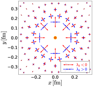
Figure 5: Stress distribution around a static quark at the origin at $T/T_{c}=2.60$. The red and blue arrows are the principal directions along the radial and transverse directions, respectively. The length of each arrow represents square root of the eigenvalue.

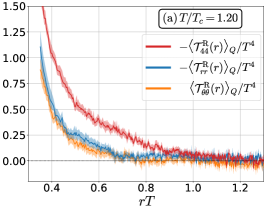
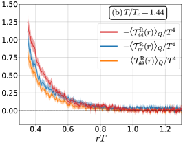
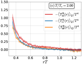
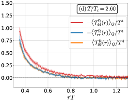
Figure 6: EMT distribution $(-\langle{\cal T}_{44}^{\mathrm{R}}(r)\rangle_{Q},-\langle{\cal T}_{rr}^{\mathrm{R}}(r)\rangle_{Q},\langle{\cal T}_{\theta\theta}^{\mathrm{R}}(r)\rangle_{Q})$ as functions of $rT$ after the double extrapolation: (a) $T=1.20T_{c}$, (b) $T=1.44T_{c}$, (c) $T=2.00T_{c}$, and (d) $T=2.60T_{c}$.

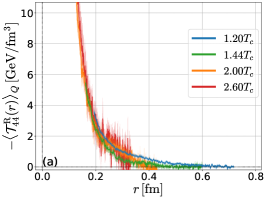
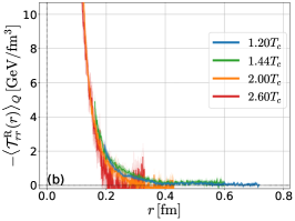
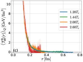
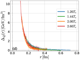
Figure 7: EMT distribution $(-\langle{\cal T}_{44}^{\mathrm{R}}(r)\rangle_{Q},-\langle{\cal T}_{rr}^{\mathrm{R}}(r)\rangle_{Q},\langle{\cal T}_{\theta\theta}^{\mathrm{R}}(r)\rangle_{Q})$ and $\Delta_{Q}(r)$ as functions of $r$ [fm] at each temperature: (a) $-\langle{\cal T}_{44}^{\mathrm{R}}(r)\rangle_{Q}$, (b) $-\langle{\cal T}_{rr}^{\mathrm{R}}(r)\rangle_{Q}$, (c) $\langle{\cal T}_{\theta\theta}^{\mathrm{R}}(r)\rangle_{Q}$, and (d) $\Delta_{Q}(r)$.

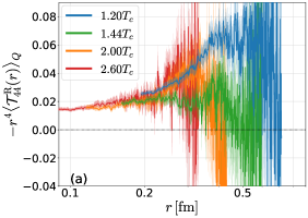
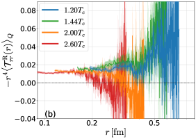
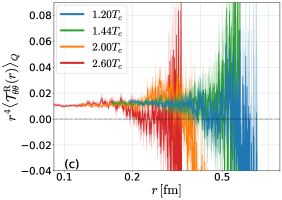
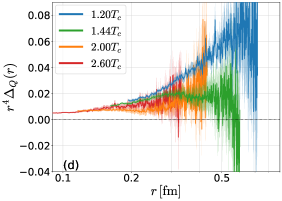
Figure 8: EMT distribution $r^{4}(-\langle{\cal T}_{44}^{\mathrm{R}}(r)\rangle_{Q},-\langle{\cal T}_{rr}^{\mathrm{R}}(r)\rangle_{Q},\langle{\cal T}_{\theta\theta}^{\mathrm{R}}(r)\rangle_{Q})$ and $r^{4}\Delta_{Q}(r)$ as functions of $r$ [fm] at each temperature: (a)$-r^{4}\langle{\cal T}_{44}^{\mathrm{R}}(r)\rangle_{Q}$, (b)$-r^{4}\langle{\cal T}_{rr}^{\mathrm{R}}(r)\rangle_{Q}$, (c)$r^{4}\langle{\cal T}_{\theta\theta}^{\mathrm{R}}(r)\rangle_{Q}$, and (d)$r^{4}\Delta_{Q}(r)$.

In Fig. 6, we show the dimensionless EMT, $-\langle{\cal T}_{44}^{\mathrm{R}}(r)\rangle_{Q}/T^{4}$, $-\langle{\cal T}_{rr}^{\mathrm{R}}(r)\rangle_{Q}/T^{4}$, and $\langle{\cal T}_{\theta\theta}^{\mathrm{R}}(r)\rangle_{Q}/T^{4}$, as functions of the dimensionless length $rT$. The error bands include both the statistical and systematic errors, where the latter is estimated from the three fitting ranges for the $t\to 0$ extrapolation. Since the thermal expectation value $\langle\mathcal{T}_{\mu\nu}(t,x)\rangle$ is subtracted as in Eq. (12), we have $\langle\mathcal{T}^{\mathrm{R}}_{\mu\nu}(r)\rangle_{Q}\to 0$ in the $r\to\infty$ limit.

We find that $-\langle{\cal T}_{44}^{\mathrm{R}}(r)\rangle_{Q}$, $-\langle{\cal T}_{rr}^{\mathrm{R}}(r)\rangle_{Q}$, and $\langle{\cal T}_{\theta\theta}^{\mathrm{R}}(r)\rangle_{Q}$ are all positive for $rT\lesssim 1$ and decrease rapidly with increasing $r$. These signs are the same as those of the Maxwell stress tensor in Eq. (5). Individual signs physically mean that a volume element has a positive localized energy density and receives a pulling (pushing) force along the longitudinal (transverse) direction; see Figs. 1 and 5.

Figure 6 indicates that the absolute values of the spatial components $|\langle{\cal T}_{rr}^{\mathrm{R}}(r)\rangle_{Q}|$ and $|\langle{\cal T}_{\theta\theta}^{\mathrm{R}}(r)\rangle_{Q}|$ are degenerated within the error for all temperatures. On the other hand, $|\langle{\cal T}_{44}^{\mathrm{R}}(r)\rangle_{Q}|$ is larger than the spatial components especially at lower temperature. This is in contrast to the degenerate magnitude of all components in the Maxwell stress Eq. (5) and is also different from the leading-order thermal perturbation theory (Appendix B).

V.2 Temperature dependence

Shown in Fig. 7 is the temperature dependence of the spatial distribution of EMT with respect to the physical distance $r$ [fm]; (a) $-\langle{\cal T}_{44}^{\mathrm{R}}(r)\rangle_{Q}$, (b) $-\langle{\cal T}_{rr}^{\mathrm{R}}(r)\rangle_{Q}$, and (c) $\langle{\cal T}_{\theta\theta}^{\mathrm{R}}(r)\rangle_{Q}$. Also, shown in Fig. 7(d) is the distribution of the trace of EMT given by

$$\Delta_{Q}(r) \equiv-\langle\mathcal{T}^{\mathrm{R}}_{\mu\mu}(r)\rangle_{Q}$$

$$=-\langle\mathcal{T}^{\mathrm{R}}_{44}(r)+\mathcal{T}^{\mathrm{R}}_{rr}(r)+2\mathcal{T}^{\mathrm{R}}_{\theta\theta}(r)\rangle_{Q}.$$ (17)

Figure 7 tells us that the EMT distributions have small $T$ dependence at short distances, $r\lesssim 0.2$ fm. On the other hand, for large distances, sizable $T$ dependence can be seen despite the growth of the errors at high $T$.

To make these features more explicit, we plot the same results with a dimensionless normalization $r^{4}\langle{\cal T}_{\gamma\gamma^{\prime}}^{\mathrm{R}}(r)\rangle_{Q}$ as a function of $r$ in Fig. 8. The figure shows that the $T$ dependence is suppressed for $rT\lesssim 0.3$ and all results approach a single line, while the result tends to be more suppressed for $rT\gtrsim 0.3$ compared with this universal behavior as temperature is raised. This result is reasonable as the $T$ dependence of $r^{4}\langle{\cal T}_{\gamma\gamma^{\prime}}^{\mathrm{R}}(r)\rangle_{Q}$ would be suppressed for $r\lesssim(2\pi T)^{-1}$.

At distance $(2\pi T)^{-1}\ll r\ll\Lambda^{-1}$ with $\Lambda$ being the lambda parameter, the behavior of $\langle{\cal T}_{\gamma\gamma^{\prime}}^{\mathrm{R}}(r)\rangle_{Q}$ should be described by the perturbation theory in electrostatic QCD (EQCD). In the leading order of EQCD in this regime, we have the following ratio (Appendix B),

$$\left|\frac{\Delta_{Q}(r)}{\langle{\cal T}^{\mathrm{R}}_{44,rr,\theta\theta}(r)\rangle_{Q}}\right|=\frac{11}{2\pi}\alpha_{s}+\mathcal{O}(g^{3}),$$ (18)

which is independent of $r$ and $T$ and is given only by a function of $\alpha_{s}$.

Shown in Fig. 9 is the $r$ dependence of $\Delta_{Q}(r)/\langle\mathcal{T}_{44,rr,\theta\theta}^{\mathrm{R}}(r)\rangle_{Q}$ as a function of $r$ at $T/T_{c}=2.60$. From this result and Eq. (18), we obtain, at $r=0.1$ fm, $\alpha_{s}=0.221(17)$ from $-\Delta_{Q}(r)/\langle{\cal T}^{\mathrm{R}}_{44}(r)\rangle_{Q}$, $\alpha_{s}=0.286(24)$ from $-\Delta_{Q}(r)/\langle{\cal T}^{\mathrm{R}}_{rr}(r)\rangle_{Q}$, and $\alpha_{s}=0.319(35)$ from $\Delta_{Q}(r)/\langle{\cal T}^{\mathrm{R}}_{\theta\theta}(r)\rangle_{Q}$. Although these values are channel dependent, indicating the existence of non-negligible higher order contributions, it is notable that they are consistent with that obtained from the similar analysis of the Polyakov loop correlations at $r=0.1$ fm Kaczmarek:2004gv ; Kaczmarek:2005ui . Higher order $\alpha_{s}$ corrections and the thermal corrections for EMT around a static charge to be compared with our lattice data is under way Matthias .

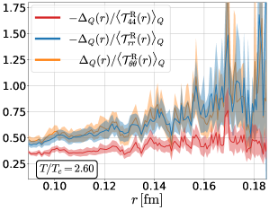
Figure 9: Ratios $\Delta_{Q}(r)/\langle\mathcal{T}_{44,rr,\theta\theta}^{\mathrm{R}}(r)\rangle_{Q}$ as functions of $r$ at $T/T_{c}=2.60$.

Let us now turn to the long-distance region in Fig. 8. Owing to the large errors in this region, it is not possible to extract the thermal screening of the form $\exp(-2m_{\rm{}_{D}}r)$ with $m_{\rm{}_{D}}$ being the Debye screening mass. Nevertheless, Figs. 8(a-d) indicate that the EMT distributions decrease faster than $1/r^{4}$ at long distances, and the tendency is stronger at high temperatures. To draw a definite conclusion, however, higher statistical data are necessary.

VI Summary and Concluding remarks

In the present paper, we have studied, for the first time, the EMT distribution around a static quark at finite temperature above $T_{c}$ of the SU(3) YM theory on the lattice. The YM gradient flow plays crucial roles to define the EMT on the lattice and to explore its spatial structure.

The main results of this paper can be summarized as follows.

As shown in Fig. 6, we found no significant difference between the absolute magnitude of EMT along the radial direction and that of the transverse direction for all temperatures above $T_{c}$. This seems to be in accordance with the leading-order thermal perturbation theory in QCD, which predicts the same magnitude for all principal components of EMT. However, we found a substantial difference between the EMT distribution in the temporal direction and that of the spatial directions, especially near $T_{c}$. This indicates that there is indeed a genuine non-Abelian effect present at finite temperature, so that precise comparison with the higher-order thermal QCD calculation would be called for.

As shown in Figs. 7 and 8, all the EMT distributions have small $T$ dependence at short distances, $r\lesssim 0.2$ fm. Also the EMT distributions decrease faster than $1/r^{4}$ at long distances, and the tendency is stronger at high temperatures. However, owing to the large statistical errors, we could not extract the values of the thermal Debye screening. By using the fact that the EMT distributions are $T$ independent at short distances, we attempted to extract the strong coupling constant from the ratios between the different components of EMT. The result, $\alpha_{s}(0.1\ {\rm fm})\simeq 0.28-0.32$, is consistent with that obtained from the similar analysis for the $Q\bar{Q}$ free energy at finite $T$.

We have some important issues to be studied further: Going beyond the leading-order thermal QCD calculation for the EMT  Matthias is necessary to understand the lattice results presented in this paper. At the same time, increasing the statistics of lattice data is necessary to extract, e.g. the screening mass from the long range part of the EMT distribution.

There are also several interesting future problems. First of all, the extension to full QCD is an important next step. Since the $Z_{3}$ symmetry is explicitly broken by dynamical fermions, the present method can be applied directly to a single static quark $Q$, a static diquark $QQ$ and $Q\bar{Q}$ both at low and high temperatures. In particular, the single quark system in QCD at zero temperature corresponds to a heavy-light meson Mueller:2019mkh . Secondly, the EMT distributions of the $QQQ$ system will provide new insight into the flux tube formation in baryons Takahashi:2002bw as well as the “gravitational” baryon structure Kumano:2017lhr ; Polyakov:2018zvc ; Burkert:2018bqq ; Shanahan:2018nnv at zero and non-zero temperatures.

Appendix A Tree-level improvement of the lattice observables

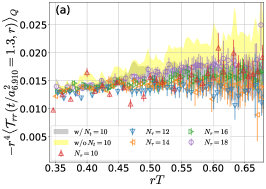
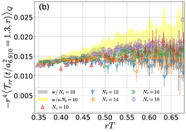
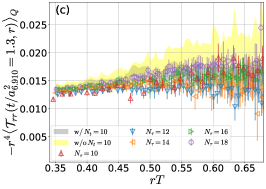
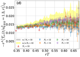
Figure 10: Distribution of $-r^{4}\langle\mathcal{T}_{rr}(t/a_{6.910}^{2}=1.3,r)\rangle_{Q}$ as functions of $rT$. (a) Same figure as Fig. 2 shown for a comparison. (b,c,d) Tree-level improved results with Eqs. (25) and (28) for three choices of $U^{\mathrm{tl}}_{\gamma\gamma^{\prime}}$: (b) $U^{\mathrm{tl}}_{\gamma\gamma^{\prime}}=\langle U_{44}\rangle_{Q}$, (c) $U^{\mathrm{tl}}_{\gamma\gamma^{\prime}}=\langle U_{rr}\rangle_{Q}$, (d) $U^{\mathrm{tl}}_{\gamma\gamma^{\prime}}=\langle U_{\theta\theta}\rangle_{Q}$.

As shown in Fig. 2, there exists sizable discretization effect for the EMT distribution on coarse lattices especially for $N_{\tau}=10$. In this Appendix, we attempt to reduce such discretization effects by using the tree-level lattice propagator. Similar idea has been applied to the analysis of the Polyakov loop correlations in Refs. Necco:2001xg ; Kaczmarek:2004gv .

In calculating the EMT distribution around a static quark Eq. (16), we need the expectation values of Eqs. (10) and (11) at nonzero flow time $t$. These quantities are constructed from $\langle G^{a}_{\mu\nu}(t,\bm{x})G^{a}_{\rho\sigma}(t,\bm{x})\rangle_{Q}$, where the temporal coordinate is suppressed for notational simplicity. In the continuum theory at the tree level, this operator is calculated to be

$$\langle G^{a}_{\mu\nu}(t,\bm{x})G^{a}_{\rho\sigma}(t,\bm{x})\rangle_{Q}=-g^{2}\frac{N^{2}-1}{2}\mathcal{G}_{\mu\nu}(t,\bm{x})\mathcal{G}_{\rho\sigma}(t,\bm{x}),$$ (19)

where $g$ is the gauge coupling and $N=3$ is the number of colors, with

$${\cal G}_{\mu\nu}(t,\bm{x})\delta^{ab}=\int_{0}^{1/T}d\tau\langle A_{4}^{a}(\tau,\bm{0})G_{\mu\nu}^{b}(t,x)\rangle.$$ (20)

By selecting appropriate gauge fixing conditions for the gauge action and the gradient flow equation, one obtains $\mathcal{G}_{12}(t,\bm{x})=\mathcal{G}_{23}(t,\bm{x})=\mathcal{G}_{31}(t,\bm{x})=0$ and

$$\mathcal{G}_{i4}(t,\bm{x})=\partial_{i}D(t,\bm{x}),$$ (21)

$$D(t,\bm{x})=\int\frac{d^{3}p}{(2\pi)^{3}}e^{i\bm{p}\cdot\bm{x}}\frac{e^{-tp^{2}}}{p^{2}}=\frac{1}{4\pi|\bm{x}|}{\rm erf}\Big{(}\frac{|\bm{x}|}{\sqrt{4t}}\Big{)}.$$ (22)

Next, in lattice gauge theory the propagator corresponding to Eq. (22) with the Wilson gauge action for the gauge action and the flow equation reads Fodor:2014cpa ; Altenkort:2020fgs

$${\cal D}(t,\bm{x}_{n})=\int_{-\pi}^{\pi}\frac{d^{3}p}{(2\pi)^{3}}e^{i\bm{p}\cdot\bm{x}_{n}}\frac{e^{-t\sum_{i}\hat{p}_{i}^{2}}}{\sum_{i}\hat{p}_{i}^{2}},$$ (23)

with $\bm{x}_{n}=a\bm{n}=a(n_{x},n_{y},n_{z})$ and $\hat{p}_{i}=(2/a)\sin(p_{i}/2a)$. When the clover-leaf operator for the discretized representation of $G_{\mu\nu}^{a}(t,\bm{x}_{n})$ is employed, the discretized representation of $\mathcal{G}_{i4}(t,\bm{x}_{n})$ is given by Fritzsch:2013je

$$\mathcal{G}^{\mathrm{lat}}_{i4}(t,\bm{x}_{n})=\frac{1}{2a}\left({\cal D}(t,\bm{x}_{n+\hat{i}})-{\cal D}(t,\bm{x}_{n-\hat{i}})\right).$$ (24)

Using Eq. (21) and (24), the tree-level improvements of Eqs. (10) and (11) denoted by the superscript ‘imp’ may be written as

$$\langle E(t,\bm{x}_{n})\rangle_{Q}^{\rm imp}=c(t,\bm{x}_{n})\langle E(t,\bm{x}_{n})\rangle_{Q},$$ (25)

$$\langle{U}_{\gamma\gamma^{\prime}}(t,\bm{x}_{n})\rangle_{Q}^{\rm imp}=c(t,\bm{x}_{n})\langle{U}_{\gamma\gamma^{\prime}}(t,\bm{x}_{n})\rangle_{Q},$$ (26)

where the correction factor $c(t,\bm{x}_{n})$ is defined by

$$c(t,\bm{x}_{n})=\frac{1}{3}\sum_{i=1}^{3}\Big{(}\frac{\mathcal{G}_{i4}(t,\bm{x}_{n})}{\mathcal{G}_{i4}^{{\rm lat}}(t,\bm{x}_{n})}\Big{)}^{2}.$$ (27)

In Eq. (27), the average over $i$ is taken because generally the ratio $\mathcal{G}_{i4}(t,\bm{x}_{n})/\mathcal{G}_{i4}^{{\rm lat}}(t,\bm{x}_{n})$ at a lattice site $\bm{x}_{n}$ depends on $i$. However, in our particular choice of discretization, i.e. the Wilson gauge actions and the clover-leaf operator, it is easily shown that $\mathcal{G}_{i4}(t,\bm{x}_{n})/\mathcal{G}_{i4}^{{\rm lat}}(t,\bm{x}_{n})$ does not depend on $i$. In this special case the average over $i$ in Eq. (27) is redundant. When this property is violated, the improvement of $\langle{U}_{\gamma\gamma^{\prime}}(t,\bm{x}_{n})\rangle_{Q}$ may be replaced by the one that depends on $\gamma$ and $\gamma^{\prime}$ in place of Eq. (26).

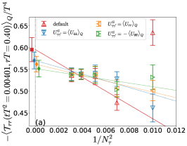
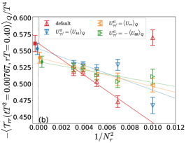
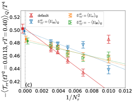
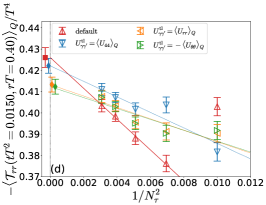
Figure 11: Comparison of the different prescriptions in the continuum extrapolation of $-\langle{\cal T}_{rr}(t,rT=0.40)\rangle_{Q}/T^{4}$ at $T/T_{c}=1.44$: (a) $tT^{2}=0.00401$, (b) $tT^{2}=0.00767$, (c) $tT^{2}=0.0113$, and (d) $tT^{2}=0.0150$.

There is one more subtle issue about Eq. (26). At the tree level, one easily finds that the matrix elements of $U_{44}$, $U_{rr}$ and $-U_{\theta\theta}$ are the same, while the actual lattice data do not necessarily satisfy such relation as shown in the main text. In our tree-level improvement, therefore, we decompose our lattice data into tree-like part and the rest, $\langle U_{\gamma\gamma^{\prime}}(t,\bm{x}_{n})\rangle_{Q}=U_{\gamma\gamma^{\prime}}^{\rm tl}(t,\bm{x}_{n})+\delta U_{\gamma\gamma^{\prime}}(t,\bm{x}_{n})$, where the tree-like part $U_{\gamma\gamma^{\prime}}^{\rm tl}(t,\bm{x}_{n})$ satisfies $U_{44}^{\rm tl}(t,\bm{x}_{n})=U^{\rm tl}_{rr}(t,\bm{x}_{n})=-U_{\theta\theta}^{\rm tl}(t,\bm{x}_{n})$. Then we apply our tree-level improvement only to the first term:

$$\langle{U}_{\gamma\gamma^{\prime}}(t,\bm{x}_{n})\rangle_{Q}^{\rm imp}=c(t,\bm{x}_{n})U_{\gamma\gamma^{\prime}}^{\rm tl}(t,\bm{x}_{n})+\delta U_{\gamma\gamma^{\prime}}(t,\bm{x}_{n}).$$ (28)

Below, we consider three choices of $U_{\gamma\gamma^{\prime}}^{\rm tl}(t,\bm{x}_{n})$ to estimate the systematic uncertainty of this procedure: $U_{\gamma\gamma^{\prime}}^{\rm tl}=\langle U_{44}\rangle_{Q},\langle U_{rr}\rangle_{Q}$, and $-\langle U_{\theta\theta}\rangle_{Q}$. Corresponding results for $\langle{\cal T}_{rr}^{\mathrm{R}}(t,r)\rangle$ as example are shown in Fig. 10(b), (c), and (d), respectively, together with the case without the correction, Fig. 10(a). Colored open symbols represent the data at each $N_{\tau}$ and the gray (yellow) shade is the continuum result with (without) the data at $N_{\tau}=10$. The figures show that the tree-level improvement suppresses the discretization effect at short distances in three cases, especially for $N_{\tau}=10$.

Let us now compare the continuum extrapolation using the data including $N_{\tau}=10$ with the tree-level improvement and that using the data without $N_{\tau}=10$ and without the tree-level improvement. Shown in Fig. 11 is such a comparison for $-\langle{\cal T}_{rr}(t,rT=0.40)\rangle_{Q}/T^{4}$ at $T/T_{c}=1.44$ as functions of $1/N_{\tau}^{2}$. Colored open triangles represent the data without the tree-level improvement (red) and with the tree-level improvement for three different prescriptions (blue, orange, and green). Filled symbols at $1/N_{\tau}^{2}=0$ are the continuum extrapolation: The red squares are continuum results without $N_{\tau}=10$ data discussed in the main text, while the diamonds are the continuum results with $N_{\tau}=10$ data after the tree-level improvement. Taking into the uncertainly associated with the different prescriptions for the tree-level improvement, the default results without $N_{\tau}=10$ in the main text are found to be consistent with the improved results including $N_{\tau}=10$.

Appendix B Leading order perturbative analysis of EMT around a static charge

Let us consider the SU($N$) Yang-Mills system at high temperature where $g(2\pi T)\ll 1$. Then, the effective theory valid at the length scale of $R\gg(2\pi T)^{-1}$ is the dimensionally reduced electrostatic QCD (EQCD) in three dimensions (see, e.g., Appelquist:1981vg ; DHoker:1981bjo ; Nadkarni:1982kb ; Braaten:1994qx )

$$S_{\rm{}_{EQCD}}=\int d^{3}x\,\Bigl{[}\frac{1}{2}\mathrm{Tr}{\cal G}^{2}+\mathrm{Tr}(D\varphi)^{2}+m_{\rm{}_{D}}^{2}\mathrm{Tr}\varphi^{2}+\delta{\cal L}_{\rm{}_{EQCD}}\Bigr{]}.$$ (29)

Here $({\cal A}_{i},\varphi)=({\cal A}^{a}_{i}t^{a},\varphi^{a}t^{a})=(A_{i},A_{4})/(g\sqrt{T})$, ${\cal G}_{ij}=\partial_{i}{\cal A}_{j}-\partial_{j}{\cal A}_{i}+ig_{\rm{}_{E}}[{\cal A}_{i},{\cal A}_{j}]$, and $D_{i}\varphi=\partial_{i}\varphi+ig_{\rm{}_{E}}[{\cal A}_{i},\varphi]$ with ${\rm Tr}(t^{a}t^{b})=\frac{1}{2}\delta^{ab}$. The higher dimensional operators are denoted by $\delta{\cal L}_{\rm{}_{EQCD}}$. The effective coupling and the Debye screening mass in the leading-order (LO) read $g_{\rm{}_{E}}=g\sqrt{T}$ and $m_{\rm{}_{D}}^{2}=(N/3)(gT)^{2}$, respectively.

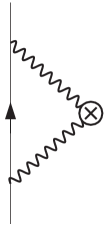
Figure 12: Diagram contributing to the leading-order calculation of the correlation function between the Polyakov loop and the EMT operator. The vertical line represents the Polyakov loop and two wavy lines exchanged gluons. The symbol $\otimes$ corresponds to the EMT operator.

Under the “Feynman static gauge” ($\partial_{4}{\cal A}_{4}=0$ for the temporal component and the Feynman gauge for the spatial component ${\cal A}_{i}$)  DHoker:1981bjo ; Nadkarni:1982kb , the tree-level propagators read

$$\langle\varphi^{a}(\bm{0})\varphi^{b}(\bm{x})\rangle=\delta_{ab}\frac{e^{-m_{\rm{}_{D}}|\bm{x}|}}{4\pi|\bm{x}|},$$ (30)

$$\langle{\cal A}_{i}^{a}(\bm{0}){\cal A}_{j}^{b}(\bm{x})\rangle=\delta_{ab}\delta_{ij}\frac{1}{4\pi|\bm{x}|},$$ (31)

$$\langle{\cal A}_{i}^{a}(\bm{0})\varphi^{b}(\bm{x})\rangle=0,$$ (32)

where $a$ and $b$ are color indices. Moreover, the Polyakov loop operator $\Omega(\bm{x})$ is written as

$$\Omega(\bm{x})=\mathcal{P}e^{-ig\int_{0}^{1/T}d\tau A_{4}(\bm{x},\tau)}=e^{-ig\varphi(\bm{x})/\sqrt{T}}.$$ (33)

The leading order (LO) contribution to the connected correlation between the Polyakov loop and the EMT stems from the two gluon exchange of $O(g^{2})$ and is diagrammatically shown in Fig. 12. Since the Polyakov loop operator has only the scalar component $\varphi(\bm{x})$, the terms which survive in the LO are the connected diagrams with $G_{4i}^{2}$, i.e.,

$$\langle(G_{i4}^{a})^{2}(\bm{x})\rangle_{Q}=\frac{\langle(G_{i4}^{a})^{2}(\bm{x})\mathrm{Tr}\Omega(\bm{0})\rangle_{c}}{\langle\mathrm{Tr}\Omega(\bm{0})\rangle},$$ (34)

where the suffix $c$ implies the connect correlation.

By expanding $(G_{i4}^{a})^{2}$ and $\mathrm{Tr}\Omega$ up to $O(\varphi^{2})$ for fixed $i=1,2,3$, we obtain

$$\langle(G_{i4}^{a})^{2}(\bm{x})\rangle_{Q}$$

$$=-\frac{1}{4N}g^{2}\langle\varphi^{a}(\bm{0})\partial_{i}\varphi^{b}(\bm{x})\rangle\langle\varphi^{b}(\bm{0})\partial_{i}\varphi^{a}(\bm{x})\rangle+\mathcal{O}(g^{3})$$

$$=-\frac{N^{2}-1}{4N}g^{2}\left\{\partial_{i}\left(\frac{e^{-m_{\rm{}_{D}}|\bm{x}|}}{4\pi|\bm{x}|}\right)\right\}^{2}+\mathcal{O}(g^{3})$$

$$=-\frac{C_{F}}{8\pi}\alpha_{s}\frac{x_{i}^{2}(m_{\rm{}_{D}}|\bm{x}|+1)^{2}}{|\bm{x}|^{6}}e^{-2m_{\rm{}_{D}}|\bm{x}|}+\mathcal{O}(g^{3}),$$ (35)

where $\alpha_{s}=g^{2}/4\pi$ and $C_{F}=(N^{2}-1)/2N$.

Picking up the contributions of $(G_{4i}^{a})^{2}(\bm{x})$ in each component of the EMT, we obtain the following perturbative estimate for $r\equiv|\bm{x}|\gg(2\pi T)^{-1}$ up to $O(g^{2})$,

$$\langle\mathcal{T}_{44}(\bm{x})\rangle_{Q}=\langle\mathcal{T}_{rr}(\bm{x})\rangle_{Q}=-\langle\mathcal{T}_{\theta\theta}(\bm{x})\rangle_{Q}$$

$$\ \ \ \ =-\frac{C_{F}}{8\pi}\alpha_{s}\frac{(m_{\rm{}_{D}}r+1)^{2}}{r^{4}}e^{-2m_{\rm{}_{D}}r}+\mathcal{O}(g^{3}),$$ (36)

Simplest way to show the above relation is to choose $\bm{x}=(r,0,0)$, so that $\mathcal{T}_{rr}(r,0,0)=\mathcal{T}_{11}(r,0,0)$ and $\mathcal{T}_{\theta\theta}(r,0,0)=\mathcal{T}_{22}(r,0,0)$.

Although one finds that the EMT trace $\langle\mathcal{T}_{\mu\mu}(\bm{x})\rangle_{Q}$ vanishes at $O(g^{2})$, one can utilize the following trace anomaly to evaluate its $O(g^{4})$ contribution:

$$\mathcal{T}_{\mu\mu}=\frac{\beta}{2g}G_{\mu\nu}^{a}G_{\mu\nu}^{a},$$ (37)

where the Yang-Mills beta function reads $\beta=-\beta_{0}g^{3}-\beta_{1}g^{5}+\cdots$, with $\beta_{0}=(11/3)C_{A}/(4\pi)^{2}$, $\beta_{1}=(34/3)C_{A}^{2}/(4\pi)^{4}$, and $C_{A}=N$. By using the right hand side of the formula and follow the same procedure as above, we find

$$\langle\mathcal{T}_{\mu\mu}(\bm{x})\rangle_{Q}=-\frac{11}{3}\frac{C_{A}C_{F}}{(4\pi)^{2}}\alpha_{s}^{2}\frac{(m_{\rm{}_{D}}r+1)^{2}}{r^{4}}e^{-2m_{\rm{}_{D}}r}+\mathcal{O}(g^{5}).$$ (38)

This is indeed $O(g^{2})$ higher than Eq. (36).

References

- (1) G. S. Bali, Phys. Rept. 343, 1 (2001).
- (2) R. Narayanan and H. Neuberger, JHEP 0603, 064 (2006) [hep-th/0601210].
- (3) M. Lüscher, JHEP 1008, 071 (2010) [arXiv:1006.4518 [hep-lat]].
- (4) M. Lüscher and P. Weisz, JHEP 1102, 051 (2011) [arXiv:1101.0963 [hep-th]].
- (5) H. Suzuki, PTEP 2013, 083B03 (2013) [Erratum: PTEP 2015, 079201 (2015)] [arXiv:1304.0533 [hep-lat]].
- (6) H. Makino and H. Suzuki, PTEP 2014, 063B02 (2014) [Erratum: PTEP 2015, 079202 (2015)] [arXiv:1403.4772 [hep-lat]].
- (7) K. Hieda, H. Makino and H. Suzuki, Nucl. Phys. B 918, 23-51 (2017) [arXiv:1604.06200 [hep-lat]].
- (8) R. V. Harlander, Y. Kluth and F. Lange, Eur. Phys. J. C 78, 944 (2018) [arXiv:1808.09837 [hep-lat]].
- (9) R. Yanagihara, T. Iritani, M. Kitazawa, M. Asakawa and T. Hatsuda, Phys. Lett. B 789, 210 (2019) [arXiv:1803.05656 [hep-lat]].
- (10) R. Yanagihara and M. Kitazawa, PTEP 2019, 093B02 (2019) [Erratum: PTEP 2020, 079201 (2020)] [arXiv:1905.10056 [hep-ph]].
- (11) M. Asakawa et al. [FlowQCD], Phys. Rev. D 90, 011501 (2014) [Erratum: Phys. Rev.92, 059902 (2015)] [arXiv:1312.7492 [hep-lat]].
- (12) M. Kitazawa, T. Iritani, M. Asakawa, T. Hatsuda, and H. Suzuki, Phys. Rev. D 94, 114512 (2016) [arXiv:1610.07810 [hep-lat]].
- (13) M. Kitazawa, T. Iritani, M. Asakawa, and T. Hatsuda, Phys. Rev. D 96, 111502 (2017) [arXiv:1708.01415 [hep-lat]].
- (14) T. Iritani, M. Kitazawa, H. Suzuki and H. Takaura, PTEP 2019, 023B02 (2019) [arXiv:1812.06444 [hep-lat]].
- (15) T. Hirakida, E. Itou and H. Kouno, PTEP 2019, 033B01 (2019) [arXiv:1805.07106 [hep-lat]].
- (16) M. Kitazawa, S. Mogliacci, I. Kolbé and W. Horowitz, Phys. Rev. D 99, 094507 (2019) [arXiv:1904.00241 [hep-lat]].
- (17) Y. Taniguchi, S. Ejiri, R. Iwami, K. Kanaya, M. Kitazawa, H. Suzuki, T. Umeda, and N. Wakabayashi, Phys. Rev. D 96, 014509 (2017) [arXiv:1609.01417 [hep-lat]].
- (18) Y. Taniguchi et al. [WHOT-QCD], Phys. Rev. D 102, 014510 (2020) [arXiv:2005.00251 [hep-lat]].
- (19) L. D. Landau and E. M. Lifshitz, “The Classical Theory of Fields” (fourth Edition) (Butterworth-Heinemann, 1980).
- (20) S. Borsanyi, S. Dürr, Z. Fodor et al., JHEP 1209, 010 (2012) [arXiv:1203.4469 [hep-lat]].
- (21) G. Parisi, R. Petronzio, and F. Rapuano, Phys. Lett. 128B, 418 (1983).
- (22) O. Kaczmarek, F. Karsch, F. Zantow and P. Petreczky, Phys. Rev. D 70, 074505 (2004) [arXiv:hep-lat/0406036 [hep-lat]].
- (23) O. Kaczmarek and F. Zantow, Phys. Rev. D 71, 114510 (2005) [arXiv:hep-lat/0503017 [hep-lat]].
- (24) M. Berwein, in preparation.
- (25) See, for example, L. Müller, O. Philipsen, C. Reisinger and M. Wagner, Phys. Rev. D 100, no.5, 054503 (2019) [arXiv:1907.01482 [hep-lat]].
- (26) T. T. Takahashi, H. Suganuma, Y. Nemoto, and H. Matsufuru, Phys. Rev. D 65, 114509 (2002) [hep-lat/0204011].
- (27) S. Kumano, Q. T. Song and O. V. Teryaev, Phys. Rev. D 97, 014020 (2018) [arXiv:1711.08088 [hep-ph]].
- (28) M. V. Polyakov and P. Schweitzer, Int. J. Mod. Phys. A 33, 1830025 (2018) [arXiv:1805.06596 [hep-ph]].
- (29) V. D. Burkert, L. Elouadrhiri and F. X. Girod, Nature 557, 396 (2018).
- (30) P. E. Shanahan and W. Detmold, Phys. Rev. Lett. 122, 072003 (2019) [arXiv:1810.07589 [nucl-th]].
- (31) S. Necco and R. Sommer, Nucl. Phys. B 622, 328-346 (2002) [arXiv:hep-lat/0108008 [hep-lat]].
- (32) Z. Fodor, K. Holland, J. Kuti, S. Mondal, D. Nogradi and C. H. Wong, JHEP 09, 018 (2014) [arXiv:1406.0827 [hep-lat]].
- (33) L. Altenkort, A. M. Eller, O. Kaczmarek, L. Mazur, G. D. Moore and H. T. Shu, [arXiv:2009.13553 [hep-lat]].
- (34) P. Fritzsch and A. Ramos, JHEP 10, 008 (2013) [arXiv:1301.4388 [hep-lat]].
- (35) T. Appelquist and R. D. Pisarski, Phys. Rev. D 23, 2305 (1981)
- (36) E. D’Hoker, Nucl. Phys. B 201, 401-428 (1982)
- (37) S. Nadkarni, Phys. Rev. D 27, 917 (1983)
- (38) E. Braaten and A. Nieto, Phys. Rev. Lett. 74, 3530 (1995) [arXiv:hep-ph/9410218 [hep-ph]].