Continuous renormalization group function from lattice simulations
Abstract
We present a real-space renormalization group transformation with continuous scale change to calculate the continuous renormalization group function in non-perturbative lattice simulations. Our method is motivated by the connection between Wilsonian renormalization group and the gradient flow transformation. It does not rely on the perturbative definition of the renormalized coupling and is also valid at non-perturbative fixed points. Although our method requires an additional extrapolation compared to traditional step scaling calculations, it has several advantages which compensates for this extra step even when applied in the vicinity of the perturbative fixed point. We illustrate our approach by calculating the function of 2-flavor QCD and show that lattice predictions from individual lattice ensembles, even without the required continuum and finite volume extrapolations, can be very close to the result of the full analysis. Thus our method provides a non-perturbative framework and intuitive understanding into the structure of strongly coupled systems, in addition to being complementary to existing lattice determinations.
Introduction
The renormalization group (RG) function encodes the energy dependence of the running coupling. While the function is scheme dependent, the number of its zeros, corresponding to infrared and ultraviolet fixed points (IRFP, UVFP), as well as the slope around the zeros are universal. The characteristic structure of the function distinguishes conformal vs. confining, asymptotically vs. infrared free, trivial vs. asymptotically safe systems Gross and Wilczek (1973); Politzer (1973); Caswell (1974); Banks and Zaks (1982); Baikov et al. (2017); Shrock (2014); Antipin and Sannino (2018); Gorbenko et al. (2018). The perturbative function of 4-dimensional non-abelian gauge-fermion systems are known up to 5-loop level in the scheme, but the perturbative expansion is unreliable at strong couplings Baikov et al. (2017); Ryttov and Shrock (2016a, 2011, b). The function calculated non-perturbatively is essential to describe strongly coupled systems whether QCD-like, within the conformal window, or infrared free.
The gradient flow (GF) renormalized coupling Narayanan and Neuberger (2006); Lüscher (2010, 2010) is used in many lattice calculations to study the non-perturbative properties of strongly coupled systems Fodor et al. (2012); Fritzsch and Ramos (2013); Fodor et al. (2014); Hasenfratz et al. (2015); Fodor et al. (2015a); Hasenfratz and Schaich (2018); Fodor et al. (2015b); Dalla Brida et al. (2017); Chiu (2016, 2017); Fodor et al. (2018a); Hasenfratz et al. (2019a); Fodor et al. (2018b); Chiu (2019); Leino et al. (2019); Hasenfratz et al. (2019b); Witzel (2019). Most lattice studies consider the discrete step-scaling function, where the GF time and corresponding energy scale are tied to the volume Fodor et al. (2012); Fritzsch and Ramos (2013); Nogradi and Patella (2016); Fodor et al. (2014). The definition of the gradient flow renormalized coupling and the steps needed to take the continuum limit are justified perturbatively. In this letter we rely on an alternative approach based on Wilsonian real-space renormalization group that is valid also at non-perturbative FPs Wilson (1971a, b); Wilson and Kogut (1974). We develop a new method to predict the continuous function of the renormalized GF coupling. This method has several advantages compared to a traditional step-scaling calculation even when applied in the basin of attraction of the GFP. This easily compensates for the one additional extrapolation required. The approach is general and equally applicable for confining, conformal, or infrared free systems.
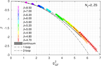
We demonstrate the method by calculating the function of a QCD-like system with two flavors and SU(3) gauge group. The final prediction of this study with relatively low statistics is shown by the grey band in Fig. 1. It is consistent with existing finite volume step scaling function calculations of 3-flavor QCD Dalla Brida et al. (2017) in that it is close to the 1-loop perturbative prediction. More interesting is that the colored data points in Fig. 1, corresponding to raw lattice data at finite volume, differ only slightly from the result of the full analysis. The continuous function approach predicts the running of the renormalized coupling in a transparent way where cut-off and finite volume effects are clearly identifiable. This property could be particularly helpful when analyzing near-conformal systems or infrared free systems where the gauge coupling at the GFP is an irrelevant parameter. GF measurements of existing configurations of step-scaling studies can be reanalyzed to predict the continuous function without additional computational cost. Hence this method provides an alternative to test systematical errors.
The connection between GF and RG is discussed in Ref. Carosso et al. (2018). Gradient flow is a continuous smearing transformation that is appropriate to define real-space RG blocked quantities, but it is not an RG transformation as it lacks the crucial step of coarse graining. However, coarse graining can be incorporated when calculating expectation values. In particular, expectation values of local operators, like the energy density that enters the definition of the GF coupling, are identical with or without coarse graining. When the dimensionless GF time is related to the RG scale change as , the GF transformation describes a continuous real-space RG transformation.
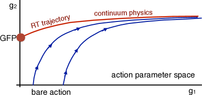
The topology of RG flow on the chiral critical surface in an asymptotically free gauge-fermion system is sketched in Fig. 2. represents the relevant gauge coupling at the Gaussian fixed point (GFP), while refers to all other irrelevant couplings. The GFP is on the (lattice spacing ) surface and the renormalized trajectory (RT) emerging from the GFP describes the cut-off independent continuum limit at finite renormalized coupling. Numerical simulations are performed with an action characterized by a set of bare couplings. If this action is in the vicinity of the GFP or its RT, the typical RG flow approaches the RT and follows it as the energy scale is decreased from the cut-off towards the infrared as indicated by the blue lines. RG flows starting at different bare couplings approach the RT differently, but once the irrelevant couplings have died out, they all follow the same 1-dimensional renormalized trajectory and describe the same continuum physics. The RT of chirally broken systems continues to , while conformal systems have an IRFP on the RT that stops the flows from either direction. While the topology of the RG space is universal, the location of the fixed points and their corresponding RTs depend on the RG transformation.
The RT is a 1-dimensional line, therefore, a dimensionless (zero canonical and zero anomalous dimension) local operator with non-vanishing expectation value can be used to define a running coupling along the RT. The simplest such quantity in gauge-fermion systems is the energy density multiplied by (or ) to compensate for its canonical dimension. This is indeed the quantity defined in Ref. Lüscher (2010) as the gradient flow coupling . , the energy density at flow time , can be estimated through various local lattice operators like the plaquette or clover operators. At large flow time irrelevant terms in the lattice definition of die out. In that limit approaches a continuum renormalized running coupling and its derivative is the RG function
| (1) |
The above definition is valid in infinite volume only. In a box of finite length the RG equation contains the term , a difficult to estimate quantity. In our approach we extrapolate at fixed which also sets the renormalization scheme . The continuum limit of the function is obtained at fixed while taking . In QCD-like systems this automatically forces the bare gauge coupling towards zero, the critical surface of the GFP.
The Wilsonian RG description suggests that lattice simulations at a single bare coupling can predict, up to controllable cut-off corrections, a finite part of the RG function. In practice the finite lattice volume limits the range where the infinite volume function is well approximated. Chaining together several bare coupling values, we can cover the entire RT while the overlap and deviation between different volume and bare coupling predictions characterizes the finite volume and finite cut-off effects as illustrated in Fig. 1.
Once the GF coupling is determined and its derivative is calculated as the function of the GF time, the continuous function calculation requires two steps:
-
A)
Infinite volume extrapolation at every GF time.
-
B)
Infinite flow time extrapolation at every .
Step B) removes cut-off effects and replaces the continuum limit extrapolation of the step-scaling function approach. Step A) is new in the continuous function approach but is compensated by several advantages. In all GF analysis the flow time has to be chosen large enough to remove all but the largest irrelevant operator even on the smallest volume considered. In traditional step-scaling calculations the flow time grows with which leads to large statistical errors on the largest volumes. In the continuous function approach the flow time is independent of the volume. This significantly reduces statistical errors. Finally the continuum limit of the continuous function is obtained by extrapolating a continuous function of the flow time. Although the data are highly correlated, a continuous function nevertheless allows control to determine the functional form, e.g. the scaling exponent of the irrelevant operator. The correlations themselves can be handled by a fully correlated analysis similar to fitting subsequent time slices of a 2-point correlation function.
The RG function is defined in the chiral limit. Finite fermion mass introduces a relevant operator that drives the RG flow away from the critical surface. Thus simulations with are essential to avoid yet another extrapolation. This is always possible in chirally symmetric conformal systems and can be enforced in chirally broken models by limiting the simulation volumes to be finite in physical units, below the inverse of the critical temperature. The same constraint is present in step-scaling studies.
A continuous function based on GF around the GFP has been considered before. The only published result is a prediction at one renormalized gauge coupling Fodor et al. (2018b) that assumes perturbative scaling.
Simulation details
Our lattice study of 2-flavor QCD is based on tree-level improved Symanzik gauge action and chirally symmetric Möbius domain wall (DW) fermions with stout smeared gauge links. Using Grid Boyle et al. (2015a, b) we generate configurations at 10 bare gauge couplings ranging from 4.70 to 8.50 on , , and volumes with fermion boundary conditions periodic in space, antiperiodic in time. In this pilot study each ensemble has between 90 to 200 measurements separated by 10 molecular dynamics time units (MDTU). The simulations are performed setting the input quark mass to zero and the 5th dimension of DW fermions to . This leads to residual masses for all gauge couplings considered. The same combination of actions has been used in recent works Hasenfratz et al. (2019a, b); Witzel et al. (2018); Witzel and Hasenfratz (2019) and properties for QCD simulations are reported in Kaneko et al. (2014); Hashimoto et al. (2014); Noaki et al. (2014); Tomiya et al. (2017). Measurements for three different gradient flows, Wilson (W), Symanzik (S), and Zeuthen (Z), have been implemented in Qlua Pochinsky (2008); Pochinsky et al. (2008) and we analyze three operators, Wilson plaquette (W), clover (C), and Symanzik (S) to estimate the energy density Sint and Ramos (2015); Ramos and Sint (2016). Our data analysis is performed using the -method which is designed to estimate and account for autocorrelations Wolff (2004).
Steps of the function calculation
In this Section we demonstrate the calculation of the continuous function step by step. Additional information including a preliminary analysis of the SU(3) system with 12 fundamental flavors can be found in Ref. Hasenfratz and Witzel (2019).
The GF coupling is defined as
| (2) |
The normalization ensures that matches the coupling at tree level, and the term corrects for the gauge zero modes due to periodic gauge boundary conditions Fodor et al. (2012). On volumes
| (3) |
where is the standard Jacobi elliptic function Fodor et al. (2012). We calculate using a symmetric 4-point numerical approximation for the derivative.
.1 Infinite volume extrapolation
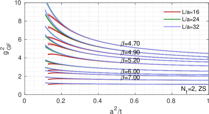
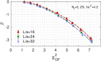

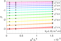
The finite volume effects depend on , and at leading order are proportional to . Figure 3 shows as the function of for our set of bare coupling values on all three volumes for Zeuthen gradient flow with Symanzik operator (ZS). The ensembles exhibit growing finite volume effects for , but the two larger volumes remain close up to . We monitor both and closely and restrict the GF time such that the finite volume corrections remain very small and the leading order term is sufficient to take the infinite volume limit.
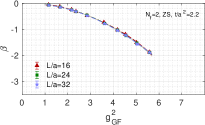
The limit has to be taken at fixed flow time and coupling . We therefore determine and its derivative on every ensemble and interpolate with a 4th order polynomial for each lattice volume to predict the finite volume function at arbitrary renormalized coupling. The top panels of Fig. 4 illustrate this for the ZS combination. We predict the infinite volume using a linear extrapolation of the interpolated values. The lower panels of Fig. 4 show examples for values spanning the accessible range in our numerical simulation. Finite volume effects are negligible at small flow time and the extrapolations are mild, well described by a linear dependence even at . As a consistency check we compare extrapolations using all three volumes to extrapolations using the two largest volumes only. While the errors of the infinite volume predictions change, the values are consistent. Other flow and operator combinations show similar volume dependence.
.2 Infinite flow time extrapolation

The final step is the continuum limit extrapolation at fixed . The GF time is a continuous variable but the range of values has to be chosen with care. First, the flow time must be large enough for the RG flow to reach the RT where irrelevant operators are suppressed. Assuming one irrelevant operator with scaling dimension dominates the cut-off effects, an extrapolation in predicts the continuum limit. Around the GFP and we find that our data is well described by a linear dependence when . Second, the upper end of the flow time range must also be restricted. When finite volume effects depending on are large, the extrapolations become unreliable. Figure 3 suggests that is sufficient to control this. Any change of the continuum limit prediction when varying the minimal and maximal flow time values can be incorporated as systematical uncertainty.
We show an example for the continuum extrapolation at in Fig. 5 where we fit the data (filled symbols) in the range (). In principle the flow time is a continuous variable; in practice we choose to dilute the data by fitting in intervals. Further we perform uncorrelated fits neglecting that values in are correlated which could easily be accounted for in a bootstrap or jackknife analysis. Varying the minimal and maximal flow times in the range impacts the uncertainties but not the central values.
We compare the functions obtained using Zeuthen flow and Wilson plaquette, Symanzik, and clover operators in Fig. 5. We consider two different infinite volume extrapolations and show for illustration additional data at larger flow time using open symbols. The linear extrapolations in shown by the colored bands are obtained independently for each operator. Their excellent agreement at the limit is a strong consistency check of the GF time range and the infinite volume extrapolation. Further consistency checks are possible by considering different flows. The scaling exponent of the leading irrelevant operator could also be extracted when performing simultaneous fits to several operators.
Discussion
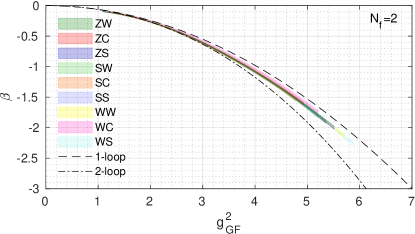
We summarize the final result of our calculation by showing in Fig. 6 the continuous GF function predicted from nine different flow and operator combinations. For reference we add the universal 1- and 2-loop perturbative predictions. The different flow/operator combinations are barely distinguishable, and the continuum limit prediction is very close to the raw ZS data as is shown in Fig. 1. The non-perturbative prediction follows the universal perturbative curves up to , but at stronger couplings is closer to the 1-loop prediction. A similar trend is observed in Ref. Dalla Brida et al. (2017); Bruno et al. (2017) for 3-flavor QCD, suggesting that the GF coupling runs slower than the coupling. Since the RG function is scheme dependent, the GF and schemes do not have to agree. However the precise non-perturbative running is needed to determine , the parameter, or connecting lattice simulations to continuum results Dalla Brida et al. (2016); Bruno et al. (2017).
The continuous function described here works in both conformal or infrared free systems Hasenfratz and Witzel (2019). The relation between GF and Wilsonian RG is especially useful in strongly coupled conformal systems. The method complements the step scaling function studies, providing a new handle on systematic errors. In addition it provides an intuitive picture to understand the RG in numerical siumlations as we show in Fig. 1.
Acknowledgements.
We are very grateful to Peter Boyle, Guido Cossu, Anontin Portelli, and Azusa Yamaguchi who develop the Grid software library providing the basis of this work and who assisted us in installing and running Grid on different architectures and computing centers. We are indebted to Daniel Nogradi for extending his original calculation on symmetric volumes to asymmetric lattices and sharing the result prior to publication. We thank Alberto Ramos for many enlightening discussions during the “37th International Symposium on Lattice Field Theory”, Wuhan, China, and Rainer Sommer and Stefan Sint for helpful comments. We benefited from many discussions with Thomas DeGrand, Ethan Neil, David Schaich, and Benjamin Svetitsky. A.H. and O.W. acknowledge support by DOE grant DE-SC0010005. A.H. would like to acknowledge the Mainz Institute for Theoretical Physics (MITP) of the Cluster of Excellence PRISMA+ (Project ID 39083149) for enabling us to complete a portion of this work. O.W. thanks the CERN theory group for their hospitality during the final stages of preparing this manuscript and acknowledges partial support by the Munich Institute for Astro- and Particle Physics (MIAPP) of the DFG cluster of excellence “Origin and Structure of the Universe”. Computations for this work were carried out in part on facilities of the USQCD Collaboration, which are funded by the Office of Science of the U.S. Department of Energy and the RMACC Summit supercomputer Anderson et al. (2017), which is supported by the National Science Foundation (awards ACI-1532235 and ACI-1532236), the University of Colorado Boulder, and Colorado State University. This work used the Extreme Science and Engineering Discovery Environment (XSEDE), which is supported by National Science Foundation grant number ACI-1548562 Towns et al. (2014) through allocation TG-PHY180005 on the XSEDE resource stampede2. This research also used resources of the National Energy Research Scientific Computing Center (NERSC), a U.S. Department of Energy Office of Science User Facility operated under Contract No. DE-AC02-05CH11231. We thank Fermilab, Jefferson Lab, NERSC, the University of Colorado Boulder, TACC, the NSF, and the U.S. DOE for providing the facilities essential for the completion of this work.References
- Gross and Wilczek (1973) D. J. Gross and F. Wilczek, Phys. Rev. D8, 3633 (1973).
- Politzer (1973) H. D. Politzer, Phys. Rev. Lett. 30, 1346 (1973).
- Caswell (1974) W. E. Caswell, Phys. Rev. Lett. 33, 244 (1974).
- Banks and Zaks (1982) T. Banks and A. Zaks, Nucl. Phys. B196, 189 (1982).
- Baikov et al. (2017) P. A. Baikov, K. G. Chetyrkin, and J. H. Kühn, Phys. Rev. Lett. 118, 082002 (2017), arXiv:1606.08659 [hep-ph] .
- Shrock (2014) R. Shrock, Phys. Rev. D89, 045019 (2014), arXiv:1311.5268 [hep-th] .
- Antipin and Sannino (2018) O. Antipin and F. Sannino, Phys. Rev. D97, 116007 (2018), arXiv:1709.02354 [hep-ph] .
- Gorbenko et al. (2018) V. Gorbenko, S. Rychkov, and B. Zan, JHEP 10, 108 (2018), arXiv:1807.11512 [hep-th] .
- Ryttov and Shrock (2016a) T. A. Ryttov and R. Shrock, Phys. Rev. D94, 105015 (2016a), arXiv:1607.06866 [hep-th] .
- Ryttov and Shrock (2011) T. A. Ryttov and R. Shrock, Phys. Rev. D83, 056011 (2011), arXiv:1011.4542 .
- Ryttov and Shrock (2016b) T. A. Ryttov and R. Shrock, Phys. Rev. D94, 125005 (2016b), arXiv:1610.00387 [hep-th] .
- Narayanan and Neuberger (2006) R. Narayanan and H. Neuberger, JHEP 0603, 064 (2006), arXiv:hep-th/0601210 [hep-th] .
- Lüscher (2010) M. Lüscher, Commun.Math.Phys. 293, 899 (2010), arXiv:0907.5491 [hep-lat] .
- Lüscher (2010) M. Lüscher, JHEP 1008, 071 (2010), arXiv:1006.4518 [hep-lat] .
- Fodor et al. (2012) Z. Fodor, K. Holland, J. Kuti, D. Nogradi, and C. H. Wong, JHEP 1211, 007 (2012), arXiv:1208.1051 [hep-lat] .
- Fritzsch and Ramos (2013) P. Fritzsch and A. Ramos, JHEP 1310, 008 (2013), arXiv:1301.4388 .
- Fodor et al. (2014) Z. Fodor, K. Holland, J. Kuti, S. Mondal, D. Nogradi, and C. H. Wong, JHEP 09, 018 (2014), arXiv:1406.0827 [hep-lat] .
- Hasenfratz et al. (2015) A. Hasenfratz, D. Schaich, and A. Veernala, JHEP 06, 143 (2015), arXiv:1410.5886 [hep-lat] .
- Fodor et al. (2015a) Z. Fodor, K. Holland, J. Kuti, S. Mondal, D. Nogradi, and C. H. Wong, JHEP 06, 019 (2015a), arXiv:1503.01132 [hep-lat] .
- Hasenfratz and Schaich (2018) A. Hasenfratz and D. Schaich, JHEP 02, 132 (2018), arXiv:1610.10004 [hep-lat] .
- Fodor et al. (2015b) Z. Fodor, K. Holland, J. Kuti, S. Mondal, D. Nogradi, and C. H. Wong, JHEP 09, 039 (2015b), arXiv:1506.06599 [hep-lat] .
- Dalla Brida et al. (2017) M. Dalla Brida, P. Fritzsch, T. Korzec, A. Ramos, S. Sint, and R. Sommer (ALPHA), Phys. Rev. D95, 014507 (2017), arXiv:1607.06423 [hep-lat] .
- Chiu (2016) T.-W. Chiu, (2016), arXiv:1603.08854 [hep-lat] .
- Chiu (2017) T.-W. Chiu, PoS LATTICE2016, 228 (2017).
- Fodor et al. (2018a) Z. Fodor, K. Holland, J. Kuti, D. Nogradi, and C. H. Wong, Phys. Lett. B779, 230 (2018a), arXiv:1710.09262 [hep-lat] .
- Hasenfratz et al. (2019a) A. Hasenfratz, C. Rebbi, and O. Witzel, Phys. Lett. B798, 134937 (2019a), arXiv:1710.11578 [hep-lat] .
- Fodor et al. (2018b) Z. Fodor, K. Holland, J. Kuti, D. Nogradi, and C. H. Wong, EPJ Web Conf. 175, 08027 (2018b), arXiv:1711.04833 [hep-lat] .
- Chiu (2019) T.-W. Chiu, Phys. Rev. D99, 014507 (2019), arXiv:1811.01729 [hep-lat] .
- Leino et al. (2019) V. Leino, T. Rindlisbacher, K. Rummukainen, F. Sannino, and K. Tuominen, (2019), arXiv:1908.04605 [hep-lat] .
- Hasenfratz et al. (2019b) A. Hasenfratz, C. Rebbi, and O. Witzel, Phys. Rev. D100, 114508 (2019b), arXiv:1909.05842 [hep-lat] .
- Witzel (2019) O. Witzel, PoS LATTICE2018, 006 (2019), arXiv:1901.08216 [hep-lat] .
- Nogradi and Patella (2016) D. Nogradi and A. Patella, Int. J. Mod. Phys. A31, 1643003 (2016), arXiv:1607.07638 [hep-lat] .
- Wilson (1971a) K. G. Wilson, Phys. Rev. B4, 3174 (1971a).
- Wilson (1971b) K. G. Wilson, Phys. Rev. B4, 3184 (1971b).
- Wilson and Kogut (1974) K. G. Wilson and J. B. Kogut, Phys. Rept. 12, 75 (1974).
- Carosso et al. (2018) A. Carosso, A. Hasenfratz, and E. T. Neil, Phys. Rev. Lett. 121, 201601 (2018), arXiv:1806.01385 [hep-lat] .
- Boyle et al. (2015a) P. Boyle, A. Yamaguchi, G. Cossu, and A. Portelli, PoS LATTICE2015, 023 (2015a), arXiv:1512.03487 [hep-lat] .
- Boyle et al. (2015b) P. Boyle, G. Cossu, A. Portelli, and A. Yamaguchi, “Grid,” (2015b).
- Witzel et al. (2018) O. Witzel, A. Hasenfratz, and C. Rebbi, (2018), arXiv:1810.01850 [hep-ph] .
- Witzel and Hasenfratz (2019) O. Witzel and A. Hasenfratz, (2019), arXiv:1912.12255 [hep-lat] .
- Kaneko et al. (2014) T. Kaneko, S. Aoki, G. Cossu, H. Fukaya, S. Hashimoto, and J. Noaki (JLQCD), PoS LATTICE2013, 125 (2014), arXiv:1311.6941 [hep-lat] .
- Hashimoto et al. (2014) S. Hashimoto, S. Aoki, G. Cossu, H. Fukaya, T. Kaneko, J. Noaki, and P. A. Boyle, PoS LATTICE2013, 431 (2014).
- Noaki et al. (2014) J. Noaki, S. Aoki, G. Cossu, H. Fukaya, S. Hashimoto, and T. Kaneko (JLQCD), PoS LATTICE2013, 263 (2014).
- Tomiya et al. (2017) A. Tomiya, G. Cossu, S. Aoki, H. Fukaya, S. Hashimoto, T. Kaneko, and J. Noaki, Phys. Rev. D96, 034509 (2017), [Addendum: Phys. Rev.D96,no.7,079902(2017)], arXiv:1612.01908 [hep-lat] .
- Pochinsky (2008) A. Pochinsky, PoS LATTICE2008, 040 (2008).
- Pochinsky et al. (2008) A. Pochinsky et al., “Qlua,” (2008).
- Sint and Ramos (2015) S. Sint and A. Ramos, PoS LATTICE2014, 329 (2015), arXiv:1411.6706 [hep-lat] .
- Ramos and Sint (2016) A. Ramos and S. Sint, Eur. Phys. J. C76, 15 (2016), arXiv:1508.05552 [hep-lat] .
- Wolff (2004) U. Wolff (ALPHA), Comput.Phys.Commun. 156, 143 (2004), arXiv:hep-lat/0306017 [hep-lat] .
- Hasenfratz and Witzel (2019) A. Hasenfratz and O. Witzel, (2019), arXiv:1911.11531 [hep-lat] .
- Bruno et al. (2017) M. Bruno, M. Dalla Brida, P. Fritzsch, T. Korzec, A. Ramos, S. Schaefer, H. Simma, S. Sint, and R. Sommer (ALPHA), Phys. Rev. Lett. 119, 102001 (2017), arXiv:1706.03821 [hep-lat] .
- Dalla Brida et al. (2016) M. Dalla Brida, P. Fritzsch, T. Korzec, A. Ramos, S. Sint, and R. Sommer (ALPHA), Phys. Rev. Lett. 117, 182001 (2016), arXiv:1604.06193 [hep-ph] .
- Anderson et al. (2017) J. Anderson, P. J. Burns, D. Milroy, P. Ruprecht, T. Hauser, and H. J. Siegel, Proceedings of PEARC17 (2017), 10.1145/3093338.3093379.
- Towns et al. (2014) J. Towns, T. Cockerill, M. Dahan, I. Foster, K. Gaither, A. Grimshaw, V. Hazlewood, S. Lathrop, D. Lifka, G. D. Peterson, R. Roskies, J. R. Scott, and N. Wilkins-Diehr, Computing in Science & Engineering 16, 62 (2014).