MPI/PhT/97–66
TTP97–40
hep-ph/9710413
October 1997

${\cal O}(\alpha_{s}^{2})$ Corrections to Top Quark Production
at $e^{+}e^{-}$ Colliders

Abstract

In this article we evaluate mass corrections up to ${\cal O}((m^{2}/q^{2})^{6})$ to the three-loop polarization function induced by an axial-vector current. Special emphasis is put on the evaluation of the singlet diagram which is absent in the vector case. As a physical application ${\cal O}(\alpha_{s}^{2})$ corrections to the production of top quarks at future $e^{+}e^{-}$ colliders is considered. It is demonstrated that for center of mass energies $\sqrt{s}\;\hbox to0.0pt{\lower 3.5pt\hbox{$\mathchar 0\relax\sim$}\hss}\raise 1.0pt\hbox{$>$}\;500$ GeV the inclusion of the first seven terms into the cross section leads to a reliable description.

PACS numbers: 12.38.-t, 12.38.Bx, 13.85.Lg, 14.65.Ha.

^aInstitut für Theoretische Teilchenphysik, Universität Karlsruhe,
D-76128 Karlsruhe, Germany,
^bMax-Planck-Institut für Physik, Werner-Heisenberg-Institut,
D-80805 Munich, Germany.

In the total cross section $\sigma(e^{+}e^{-}\to\mbox{hadrons})$ corrections arising from the finite mass, $m$, of the produced quarks may often be neglected. Concerning precision measurements around the $Z$ resonance first order mass corrections, known up to ${\cal O}(\alpha_{s}^{3})$ [1, 2], are usually adequate. However, having in mind top quark production at future colliders like the NLC with a center of mass energy of $\sqrt{s}=500$ GeV higher order terms in $m^{2}/s$ may become important. The velocity of the produced particles is then $v\approx 0.7$ which means that on one side threshold effects are not important and on the other side we are not in the region of very high energies.

In Ref. [3] the contribution of the photon to the production of top quarks was considered. In this article also the exchange of the $Z$ boson is included. Hence, in a first step results for the axial-vector polarization function up to ${\cal O}(\alpha_{s}^{2})$ are presented. The imaginary part in combination with the recently evaluated rate for the vector case [4] directly leads to the cross section $\sigma(e^{+}e^{-}\to t\bar{t}+X)$ mediated by a virtual $Z$ boson. The ${\cal O}(\alpha_{s})$ corrections to this process were considered in [5].

To be more precise let us define the axial-vector current correlator as:

$$\left(-q^{2}g_{\mu\nu}+q_{\mu}q_{\nu}\right)\,\Pi^{a}(q^{2})+q_{\mu}q_{\nu}\,\Pi^{a}_{L}(q^{2}) = i\int dx\,e^{iqx}\langle 0|Tj^{a}_{\mu}(x)j^{a}_{\nu}(0)|0\rangle$$ (1)

with $j_{\mu}^{a}=\bar{\psi}\gamma_{\mu}\gamma_{5}\psi.$ In the following we will only present results for $\Pi^{a}(q^{2})$. It is convenient to write

$$\Pi^{a}(q^{2}) = \Pi^{(0),a}(q^{2})+\frac{\alpha_{s}(\mu^{2})}{\pi}C_{F}\Pi^{(1),a}(q^{2})+\left(\frac{\alpha_{s}(\mu^{2})}{\pi}\right)^{2}\Pi^{(2),a}(q^{2})+\ldots\,\,,$$

$$\Pi^{(2),a} = C_{F}^{2}\Pi_{A}^{(2),a}+C_{A}C_{F}\Pi_{\it NA}^{(2),a}+C_{F}Tn_{l}\Pi_{l}^{(2),a}+C_{F}T\Pi_{F}^{(2),a},$$ (2)

with the $SU(3)$ colour factors $C_{F}=4/3,C_{A}=3$ and $T=1/2$. $\Pi_{A}^{(2),a}$ is the abelian contribution already present in QED and $\Pi_{NA}^{(2),a}$ originates from the non-abelian structure specific for QCD. The polarization functions containing a second massless or massive quark loop are denoted by $\Pi_{l}^{(2),a}$ and $\Pi_{F}^{(2),a}$, respectively. $\Pi^{a}$ represents the so-called non-singlet part. However, for external axial-vector currents already at ${\cal O}(\alpha_{s}^{2})$ there exists also a singlet or double-triangle contribution:

$$\Pi_{S}^{a}(q^{2}) = \left(\frac{\alpha_{s}(\mu^{2})}{\pi}\right)^{2}\,C_{F}T\,\Pi_{S}^{(2),a}(q^{2}).$$ (3)

As $\Pi_{S}^{a}$ depends on the properties of both members of the fermion doublet we will from now on specify to the top-bottom case. The generalization to other quark flavours is obvious. For this contribution it is convenient to replace the current $j^{a}_{\mu}$ in Eq. (1) by $\bar{t}\gamma_{\mu}\gamma_{5}t-\bar{b}\gamma_{\mu}\gamma_{5}b$ because in this combination the axial anomaly cancels. In Fig. 1 the relevant diagrams are depicted.

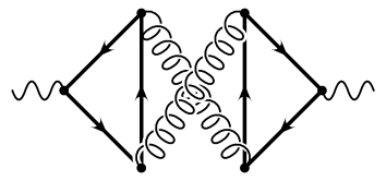
Figure 1: Diagrams contributing to $\Pi_{S}^{a}$. In the triangle loops either a top or bottom quark may be present.

Similar relations as in Eqs. (2) and (3) also hold for $R^{a}(s)$ and $R_{S}^{a}(s)$, respectively, defined through

$$R_{(S)}^{a}(s) = 12\pi\,\mbox{Im}\,\Pi_{(S)}^{a}(q^{2}=s+i\epsilon),$$ (4)

so that the cross section for the inclusive production of top quarks may be written as

$$R_{t}(s) = \frac{\sigma(e^{+}e^{-}\to t\bar{t}+X)}{\sigma_{pt}}$$ (5)

$$= (v_{e}^{2}+a_{e}^{2})a_{t}^{2}\left(\frac{s}{s-M_{Z}^{2}}\right)^{2}\,\,\left(R^{a}(s)+R_{S}^{a}(s)-\left(\frac{\alpha_{s}}{\pi}\right)^{2}C_{F}TR^{(2),a}_{Sb}(s)\right)$$

$$\mbox{}+\bigg{[}Q_{e}^{2}Q_{t}^{2}+2Q_{e}v_{e}Q_{t}v_{t}\frac{s}{s-M_{Z}^{2}}+(v_{e}^{2}+a_{e}^{2})v_{t}^{2}\left(\frac{s}{s-M_{Z}^{2}}\right)^{2}\bigg{]}\,\,R^{v}(s),$$

with $\sigma_{pt}=4\pi\alpha^{2}/3s$, $v_{f}=(I_{3}^{f}-2Q_{f}s_{\theta}^{2})/(2s_{\theta}c_{\theta})$, $a_{f}=I_{3}^{f}/(2s_{\theta}c_{\theta})$, $Q_{e}=-1,Q_{t}=2/3,I_{3}^{e}=-1/2$ and $I_{3}^{t}=1/2$. Furthermore we have $c_{\theta}^{2}=1-s_{\theta}^{2}$ with $s_{\theta}$ being the sine of the weak mixing angle. $R^{v}(s)$ is given in [4] and both $R^{a}(s)$ and $R_{S}^{a}(s)$ will be presented below. $R_{Sb}^{(2),a}$ is the contribution from cuts of the singlet diagram that do not involve top quarks. Non-singlet contributions with the photon or $Z$ boson coupling to a light quark flavour and the top quarks produced via gluon splitting [7] will be neglected as their numerical values are tiny [3].

The computation of $\Pi^{a}$ naturally splits into two parts: Firstly into the non-singlet contribution where the anticommuting definition of $\gamma_{5}$ may be used. Here the calculation of the diagrams is in close analogy to the vector case. Hence we refer for details to [4].

The second part, the singlet contribution $\Pi_{S}^{a}$, is connected with the axial anomaly and is not present in $\Pi^{v}$. Let us briefly describe our treatment of these diagrams. Actually three graphs have to be considered, namely the cases when two top quarks, one top and one bottom quark or two bottom quarks are running in the triangle loops. One may argue that the last combination only contributes to the cross section into bottom quarks which is not the process under consideration. However, only the proper combination of all three parts guarantees the cancellation of the anomaly. From the final result the cuts arising from bottom quarks have to be subtracted, of course.

For the evaluation of $\Pi_{S}^{(2),a}$ naive $\gamma_{5}$ fails to work. We follow the treatment introduced in [8] and formalized in [9] and replace both axial-vector vertices according to [10]

$$\gamma_{\mu}\gamma_{5} \to \frac{i}{3!}\,\epsilon_{\mu\lambda\rho\sigma}\gamma^{[\lambda\rho\sigma]},$$ (6)

where $\gamma^{[\lambda\rho\sigma]}$ is the antisymmetric combination of three $\gamma$ matrices which can be written as $\gamma^{[\lambda\rho\sigma]}=(\gamma^{\lambda}\gamma^{\rho}\gamma^{\sigma}-\gamma^{\sigma}\gamma^{\rho}\gamma^{\lambda})/2$. In a first step the $\epsilon$-tensors are put aside and the new object with six external indices, $\Pi^{[\lambda\rho\sigma]}_{[\lambda^{\prime}\rho^{\prime}\sigma^{\prime}]}$, defined through

$$\Pi_{\mu\nu}=\left(\frac{i}{3!}\right)^{2}\epsilon_{\mu\lambda\rho\sigma}\,\epsilon_{\nu}{}^{\lambda^{\prime}\rho^{\prime}\sigma^{\prime}}\,\Pi^{[\nu\rho\sigma]}_{[\nu^{\prime}\rho^{\prime}\sigma^{\prime}]},$$ (7)

is treated until the momentum integration and renormalization is done and a finite quantity is available [11]. Then the contraction with the $\epsilon$-tensors is performed. It is possible to show that the contribution from the singlet diagrams may be computed from the relation [12]

$$\Pi^{a}_{S}(q^{2}) = -\frac{q_{\sigma}q^{\sigma^{\prime}}\Pi^{[\lambda\rho\sigma]}_{[\lambda\rho\sigma^{\prime}]}}{6(q^{2})^{2}},$$ (8)

which means that we can treat the scalar quantity $q_{\sigma}q^{\sigma^{\prime}}\Pi^{[\nu\rho\sigma]}_{[\nu\rho\sigma^{\prime}]}$ in complete analogy to the non-singlet diagrams. We should mention that a finite renormalization of the singlet axial-vector current [13] has not to be performed in the order considered in this paper.

Using the large momentum procedure the first seven terms in the $m^{2}/q^{2}$-expansion of $\Pi^{a}(q^{2})$ have been evaluated. We refrain from listing the results separated into the contributions from the different colour factors and present the results for the proper sum keeping only $n_{l}$, the number of light (massless) quarks, as arbitrary parameter ($l_{qm}\equiv\ln(-q^{2}/m_{t}^{2})$, $l_{q\mu}\equiv\ln(-q^{2}/\mu^{2})$):

$$\bar{\Pi}^{(0),a} = {3\over 16\pi^{2}}\bigg{\{}{20\over 9}-{4\over 3}\,l_{q\mu}+{m_{t}^{2}\over q^{2}}\,\left(-8+8\,l_{q\mu}\right)+\left({m_{t}^{2}\over q^{2}}\right)^{2}\,\left(-12-8\,l_{qm}\right)$$ (9)

$$\mbox{}+\left({m_{t}^{2}\over q^{2}}\right)^{3}\,\left({8\over 9}-{16\over 3}\,l_{qm}\right)+\left({m_{t}^{2}\over q^{2}}\right)^{4}\,\left({14\over 3}-8\,l_{qm}\right)$$

$$\mbox{}+\left({m_{t}^{2}\over q^{2}}\right)^{5}\,\left({188\over 15}-16\,l_{qm}\right)+\left({m_{t}^{2}\over q^{2}}\right)^{6}\,\left({1516\over 45}-{112\over 3}\,l_{qm}\right)\bigg{\}}+\ldots\,\,,$$

$$\bar{\Pi}^{(1),a} = {3\over 16\pi^{2}}\bigg{\{}{55\over 12}-4\,\zeta_{3}-l_{q\mu}$$ (10)

$$\mbox{}+{m_{t}^{2}\over q^{2}}\,\bigg{[}-{107\over 2}+24\,\zeta_{3}+22\,l_{q\mu}-6\,l_{q\mu}^{2}\bigg{]}$$

$$\mbox{}+\left({m_{t}^{2}\over q^{2}}\right)^{2}\,\bigg{[}{2\over 3}-32\,\zeta_{3}-34\,l_{qm}-12\,l_{qm}^{2}+\left(24+24\,l_{qm}\right)\,l_{q\mu}\bigg{]}$$

$$\mbox{}+\left({m_{t}^{2}\over q^{2}}\right)^{3}\,\bigg{[}-{304\over 27}-{868\over 27}\,l_{qm}-{160\over 9}\,l_{qm}^{2}+\left(-12+24\,l_{qm}\right)\,l_{q\mu}\bigg{]}$$

$$\mbox{}+\left({m_{t}^{2}\over q^{2}}\right)^{4}\,\bigg{[}{5671\over 216}-{449\over 9}\,l_{qm}-33\,l_{qm}^{2}+\left(-40+48\,l_{qm}\right)\,l_{q\mu}\bigg{]}$$

$$\mbox{}+\left({m_{t}^{2}\over q^{2}}\right)^{5}\,\bigg{[}{1718971\over 13500}-{77954\over 675}\,l_{qm}-{3922\over 45}\,l_{qm}^{2}+\left(-118+120\,l_{qm}\right)\,l_{q\mu}\bigg{]}$$

$$\mbox{}+\left({m_{t}^{2}\over q^{2}}\right)^{6}\,\bigg{[}{9302591\over 20250}-{193546\over 675}\,l_{qm}-{11308\over 45}\,l_{qm}^{2}$$

$$\mbox{\hskip 14.22636pt}+\left(-{1796\over 5}+336\,l_{qm}\right)\,l_{q\mu}\bigg{]}\bigg{\}}+\ldots\,\,,$$

$$\bar{\Pi}^{(2),a} = {3\over 16\pi^{2}}\bigg{\{}{118379\over 1944}-{1582\over 27}\,\zeta_{3}+{100\over 9}\,\zeta_{5}+\left(-{343\over 18}+{124\over 9}\,\zeta_{3}\right)\,l_{q\mu}+{31\over 18}\,l_{q\mu}^{2}$$ (11)

$$\mbox{\hskip 14.22636pt}+n_{l}\left(-{3701\over 972}+{76\over 27}\,\zeta_{3}+\left({11\over 9}-{8\over 9}\,\zeta_{3}\right)\,l_{q\mu}-{1\over 9}\,l_{q\mu}^{2}\right)$$

$$\mbox{}+{m_{t}^{2}\over q^{2}}\,\bigg{[}-{18973\over 27}+{4612\over 9}\,\zeta_{3}+2\,\zeta_{4}-220\,\zeta_{5}$$

$$\mbox{\hskip 14.22636pt}+\left({7919\over 18}-{452\over 3}\,\zeta_{3}\right)\,l_{q\mu}-{898\over 9}\,l_{q\mu}^{2}+{110\over 9}\,l_{q\mu}^{3}$$

$$\mbox{\hskip 14.22636pt}+n_{l}\left({857\over 27}-{128\over 9}\,\zeta_{3}+\left(-{151\over 9}+{16\over 3}\,\zeta_{3}\right)\,l_{q\mu}+{32\over 9}\,l_{q\mu}^{2}-{4\over 9}\,l_{q\mu}^{3}\right)\bigg{]}$$

$$\mbox{}+\left({m_{t}^{2}\over q^{2}}\right)^{2}\,\bigg{[}{8615\over 162}-{9140\over 27}\,\zeta_{3}-{32\over 3}\,\zeta_{4}-{3080\over 27}\,\zeta_{5}+{16\over 9}\,B_{4}$$

$$\mbox{\hskip 14.22636pt}+\left(-{10987\over 27}+{32\over 3}\,\zeta_{3}\right)\,l_{qm}-{1430\over 9}\,l_{qm}^{2}-{316\over 9}\,l_{qm}^{3}$$

$$\mbox{\hskip 14.22636pt}+\left({910\over 27}+{2528\over 9}\,\zeta_{3}+{1094\over 3}\,l_{qm}+{316\over 3}\,l_{qm}^{2}\right)\,l_{q\mu}+\left(-{220\over 3}-{316\over 3}\,l_{qm}\right)\,l_{q\mu}^{2}$$

$$\mbox{\hskip 14.22636pt}+n_{l}\Bigg{(}-{149\over 81}+{416\over 27}\,\zeta_{3}+{362\over 27}\,l_{qm}+{40\over 9}\,l_{qm}^{2}+{8\over 9}\,l_{qm}^{3}$$

$$\mbox{\hskip 14.22636pt}+\left(-{116\over 27}-{64\over 9}\,\zeta_{3}-12\,l_{qm}-{8\over 3}\,l_{qm}^{2}\right)\,l_{q\mu}+\left({8\over 3}+{8\over 3}\,l_{qm}\right)\,l_{q\mu}^{2}\Bigg{)}\bigg{]}$$

$$\mbox{}+\left({m_{t}^{2}\over q^{2}}\right)^{3}\,\bigg{[}{748169\over 26244}-{18718\over 81}\,\zeta_{3}-{64\over 9}\,\zeta_{4}-{920\over 27}\,\zeta_{5}+{32\over 27}\,B_{4}$$

$$\mbox{\hskip 14.22636pt}+\left(-{639715\over 1458}-{976\over 27}\,\zeta_{3}\right)\,l_{qm}-{66698\over 243}\,l_{qm}^{2}-{55064\over 729}\,l_{qm}^{3}$$

$$\mbox{\hskip 14.22636pt}+\left(-{5342\over 243}+{98008\over 243}\,l_{qm}+{16480\over 81}\,l_{qm}^{2}\right)\,l_{q\mu}+\left({302\over 3}-{412\over 3}\,l_{qm}\right)\,l_{q\mu}^{2}$$

$$\mbox{\hskip 14.22636pt}+n_{l}\Bigg{(}-{3167\over 2187}+{224\over 27}\,\zeta_{3}+{10630\over 729}\,l_{qm}+{512\over 81}\,l_{qm}^{2}+{176\over 243}\,l_{qm}^{3}$$

$$\mbox{\hskip 14.22636pt}+\left(-{68\over 243}-{2816\over 243}\,l_{qm}-{320\over 81}\,l_{qm}^{2}\right)\,l_{q\mu}+\left(-{4\over 3}+{8\over 3}\,l_{qm}\right)\,l_{q\mu}^{2}\Bigg{)}\bigg{]}$$

$$\mbox{}+\left({m_{t}^{2}\over q^{2}}\right)^{4}\,\bigg{[}{88895269\over 209952}-{66964\over 243}\,\zeta_{3}-{32\over 3}\,\zeta_{4}-{560\over 27}\,\zeta_{5}+{16\over 9}\,B_{4}$$

$$\mbox{\hskip 14.22636pt}+\left(-{14315023\over 17496}+{64\over 9}\,\zeta_{3}\right)\,l_{qm}-{422909\over 729}\,l_{qm}^{2}-{122420\over 729}\,l_{qm}^{3}$$

$$\mbox{\hskip 14.22636pt}+\left(-{1400761\over 1944}+{63863\over 81}\,l_{qm}+{1397\over 3}\,l_{qm}^{2}\right)\,l_{q\mu}+\left({3116\over 9}-{1016\over 3}\,l_{qm}\right)\,l_{q\mu}^{2}$$

$$\mbox{\hskip 14.22636pt}+n_{l}\Bigg{(}-{65785\over 5832}+{80\over 9}\,\zeta_{3}+{12431\over 486}\,l_{qm}+{671\over 54}\,l_{qm}^{2}+{38\over 27}\,l_{qm}^{3}$$

$$\mbox{\hskip 14.22636pt}+\left({12871\over 972}-{1618\over 81}\,l_{qm}-{22\over 3}\,l_{qm}^{2}\right)\,l_{q\mu}+\left(-{40\over 9}+{16\over 3}\,l_{qm}\right)\,l_{q\mu}^{2}\bigg{)}\bigg{]}$$

$$\mbox{}+\left({m_{t}^{2}\over q^{2}}\right)^{5}\,\bigg{[}{1098529906403\over 524880000}-{4485269\over 12150}\,\zeta_{3}-{64\over 3}\,\zeta_{4}-{1120\over 27}\,\zeta_{5}+{32\over 9}\,B_{4}$$

$$\mbox{\hskip 14.22636pt}+\left(-{1102325809\over 540000}+{148\over 3}\,\zeta_{3}\right)\,l_{qm}-{1318561453\over 729000}\,l_{qm}^{2}-{9340049\over 18225}\,l_{qm}^{3}$$

$$\mbox{\hskip 14.22636pt}+\left(-{374774041\over 121500}+{12902714\over 6075}\,l_{qm}+{592222\over 405}\,l_{qm}^{2}\right)\,l_{q\mu}$$

$$\mbox{\hskip 14.22636pt}+\left({10349\over 9}-{3020\over 3}\,l_{qm}\right)\,l_{q\mu}^{2}$$

$$\mbox{\hskip 14.22636pt}+n_{l}\Bigg{(}-{124701659\over 2733750}+{1376\over 135}\,\zeta_{3}+{1173494\over 18225}\,l_{qm}+{68779\over 2025}\,l_{qm}^{2}+{4244\over 1215}\,l_{qm}^{3}$$

$$\mbox{\hskip 14.22636pt}+\left({3046471\over 60750}-{290908\over 6075}\,l_{qm}-{7844\over 405}\,l_{qm}^{2}\right)\,l_{q\mu}+\left(-{118\over 9}+{40\over 3}\,l_{qm}\right)\,l_{q\mu}^{2}\Bigg{)}\bigg{]}$$

$$\mbox{}+\left({m_{t}^{2}\over q^{2}}\right)^{6}\,\bigg{[}{2399908800637\over 262440000}-{366236\over 1215}\,\zeta_{3}-{448\over 9}\,\zeta_{4}-{1120\over 9}\,\zeta_{5}+{224\over 27}\,B_{4}$$

$$\mbox{\hskip 14.22636pt}+\left(-{114901711063\over 21870000}+{7904\over 45}\,\zeta_{3}\right)\,l_{qm}-{4577019727\over 729000}\,l_{qm}^{2}-{659557\over 405}\,l_{qm}^{3}$$

$$\mbox{\hskip 14.22636pt}+\left(-{424502089\over 36450}+{7360838\over 1215}\,l_{qm}+{395780\over 81}\,l_{qm}^{2}\right)\,l_{q\mu}$$

$$\mbox{\hskip 14.22636pt}+\left({35462\over 9}-{9800\over 3}\,l_{qm}\right)\,l_{q\mu}^{2}$$

$$\mbox{\hskip 14.22636pt}+n_{l}\Bigg{(}-{242108108\over 1366875}+{5312\over 405}\,\zeta_{3}+{114707\over 675}\,l_{qm}+{623728\over 6075}\,l_{qm}^{2}+{11896\over 1215}\,l_{qm}^{3}$$

$$\mbox{\hskip 14.22636pt}+\left({15364091\over 91125}-{765092\over 6075}\,l_{qm}-{22616\over 405}\,l_{qm}^{2}\right)\,l_{q\mu}$$

$$\mbox{\hskip 14.22636pt}+\left(-{1796\over 45}+{112\over 3}\,l_{qm}\right)\,l_{q\mu}^{2}\Bigg{)}\bigg{]}\bigg{\}}+\ldots\,\,,$$

$$\bar{\Pi}^{(2),a}_{S} = {3\over 16\pi^{2}}\bigg{\{}\left({m_{t}^{2}\over q^{2}}\right)^{2}\,\bigg{[}-{80\over 3}\,\zeta_{3}+{320\over 3}\,\zeta_{5}\bigg{]}$$ (12)

$$\mbox{}+\left({m_{t}^{2}\over q^{2}}\right)^{3}\,\bigg{[}{380\over 3}-64\,\zeta_{3}+\left({296\over 3}-32\,\zeta_{3}\right)\,l_{qm}+24\,l_{qm}^{2}\bigg{]}$$

$$\mbox{}+\left({m_{t}^{2}\over q^{2}}\right)^{4}\,\bigg{[}-{3271\over 243}-{416\over 9}\,\zeta_{3}+\left({280\over 27}+32\,\zeta_{3}\right)\,l_{qm}+{410\over 27}\,l_{qm}^{2}-{176\over 27}\,l_{qm}^{3}\bigg{]}$$

$$\mbox{}+\left({m_{t}^{2}\over q^{2}}\right)^{5}\,\bigg{[}-{395921\over 2916}-{5584\over 27}\,\zeta_{3}$$

$$\mbox{\hskip 14.22636pt}+\left({4111\over 54}+{160\over 3}\,\zeta_{3}\right)\,l_{qm}+{1340\over 9}\,l_{qm}^{2}-{1660\over 81}\,l_{qm}^{3}\bigg{]}$$

$$\mbox{}+\left({m_{t}^{2}\over q^{2}}\right)^{6}\,\bigg{[}-{105441373\over 101250}-{2420\over 3}\,\zeta_{3}$$

$$\mbox{\hskip 14.22636pt}+\left(-{6044237\over 40500}+112\,\zeta_{3}\right)\,l_{qm}+{1177331\over 1350}\,l_{qm}^{2}-{15542\over 135}\,l_{qm}^{3}\bigg{]}\bigg{\}}+\ldots\,\,,$$

where $m_{t}$ is the $\overline{\mbox{MS}}$ top mass and $\zeta$ is Riemann’s zeta-function with the values $\zeta_{2}=\pi^{2}/6$, $\zeta_{3}\approx 1.20206$, $\zeta_{4}=\pi^{4}/90$ and $\zeta_{5}\approx 1.03693$. $B_{4}\approx-1.76280$ is a constant typical for massive three-loop integrals [14]. The expansion of the two-loop quantity, $\bar{\Pi}^{(1),a}$ can be compared with the exact result [15]. At order $\alpha_{s}^{2}$ the constant and quadratic terms are in agreement with [16, 17]. Note that in the non-singlet contribution $m_{t}$ could be replaced by any other quark mass. The singlet part, however, gets modified if both quarks have to be considered as massive and even vanishes for a degenerate quark doublet. This is also the reason for the absence of the first two terms in the expansion for $m_{t}^{2}/q^{2}\to 0$: For $m_{t}=0$ the top and bottom quark are trivially degenerate and the contribution to the first order power corrections arise from a simple expansion of the diagrams for small masses. According to the structure of the $\gamma$ matrices from each triangle at least a factor $m_{t}^{2}$ has to come. This means that the $m_{t}^{2}/q^{2}$ corrections from the diagrams with two top triangles cancel against the one with a top and a bottom triangle which has an overall factor of two.

Taking the imaginary part of Eqs. (9-12) and transforming the result into the on-shell scheme concerning the top mass [18] leads to ($L_{ms}\equiv\ln(M_{t}^{2}/s)$):

$$R^{(0),a} = 3\bigg{\{}1-6\frac{M_{t}^{2}}{s}+6\left(\frac{M_{t}^{2}}{s}\right)^{2}+4\left(\frac{M_{t}^{2}}{s}\right)^{3}$$ (13)

$$\mbox{}+6\left(\frac{M_{t}^{2}}{s}\right)^{4}+12\left(\frac{M_{t}^{2}}{s}\right)^{5}+28\left(\frac{M_{t}^{2}}{s}\right)^{6}\bigg{\}}+\ldots\,\,,$$

$$R^{(1),a} = 3\bigg{\{}{3\over 4}+{M_{t}^{2}\over s}\,\left(-{9\over 2}-9\,L_{ms}\right)+\left({M_{t}^{2}\over s}\right)^{2}\,\left(-{33\over 2}+18\,L_{ms}\right)$$ (14)

$$\mbox{}+\left({M_{t}^{2}\over s}\right)^{3}\,\left({82\over 9}+{28\over 3}\,L_{ms}\right)+\left({M_{t}^{2}\over s}\right)^{4}\,\left({233\over 12}+{45\over 2}\,L_{ms}\right)$$

$$\mbox{}+\left({M_{t}^{2}\over s}\right)^{5}\,\left({12401\over 225}+{739\over 15}\,L_{ms}\right)+\left({M_{t}^{2}\over s}\right)^{6}\,\left({66803\over 450}+{1906\over 15}\,L_{ms}\right)\bigg{\}}+\ldots\,\,,$$

$$R^{(2),a} = 3\bigg{\{}{343\over 24}-{31\over 3}\,\zeta_{3}+n_{l}\,\left(-{11\over 12}+{2\over 3}\,\zeta_{3}\right)$$ (15)

$$\mbox{}+{M_{t}^{2}\over s}\,\bigg{[}-{937\over 6}+\left(79+8\,\ln 2\right)\,\zeta_{2}+111\,\zeta_{3}-{613\over 6}\,L_{ms}+{7\over 2}\,L_{ms}^{2}$$

$$\mbox{\hskip 14.22636pt}+n_{l}\,\left({20\over 3}-6\,\zeta_{2}-4\,\zeta_{3}+{13\over 3}\,L_{ms}-L_{ms}^{2}\right)\bigg{]}$$

$$\mbox{}+\left({M_{t}^{2}\over s}\right)^{2}\,\bigg{[}39+\left(-206-16\,\ln 2\right)\,\zeta_{2}-{644\over 3}\,\zeta_{3}+{255\over 2}\,L_{ms}+17\,L_{ms}^{2}$$

$$\mbox{\hskip 14.22636pt}+n_{l}\,\left(5+12\,\zeta_{2}+{16\over 3}\,\zeta_{3}-11\,L_{ms}+2\,L_{ms}^{2}\right)\bigg{]}$$

$$\mbox{}+\left({M_{t}^{2}\over s}\right)^{3}\,\bigg{[}-{236639\over 1944}+\left(-{7318\over 81}-16\,\ln 2\right)\,\zeta_{2}+{280\over 9}\,\zeta_{3}$$

$$\mbox{\hskip 14.22636pt}+{640\over 3}\,L_{ms}-{889\over 81}\,L_{ms}^{2}+n_{l}\,\left({269\over 243}+{148\over 27}\,\zeta_{2}-{638\over 81}\,L_{ms}+{10\over 3}\,L_{ms}^{2}\right)\bigg{]}$$

$$\mbox{}+\left({M_{t}^{2}\over s}\right)^{4}\,\bigg{[}{28244\over 729}+\left(-{45389\over 162}-32\,\ln 2\right)\,\zeta_{2}+{8\over 3}\,\zeta_{3}+{432461\over 972}\,L_{ms}+{4727\over 324}\,L_{ms}^{2}$$

$$\mbox{\hskip 14.22636pt}+n_{l}\,\left(-{7061\over 1296}+{40\over 3}\,\zeta_{2}-{1477\over 108}\,L_{ms}+{19\over 3}\,L_{ms}^{2}\right)\bigg{]}$$

$$\mbox{}+\left({M_{t}^{2}\over s}\right)^{5}\,\bigg{[}{1248859307\over 2160000}+\left(-{2008559\over 4050}-80\,\ln 2\right)\,\zeta_{2}-17\,\zeta_{3}$$

$$\mbox{\hskip 14.22636pt}+{550105787\over 486000}\,L_{ms}-{337981\over 8100}\,L_{ms}^{2}$$

$$\mbox{\hskip 14.22636pt}+n_{l}\,\left(-{6496853\over 243000}+{3856\over 135}\,\zeta_{2}-{114617\over 4050}\,L_{ms}+{50\over 3}\,L_{ms}^{2}\right)\bigg{]}$$

$$\mbox{}+\left({M_{t}^{2}\over s}\right)^{6}\,\bigg{[}{74282645263\over 29160000}+\left(-{21379\over 30}-224\,\ln 2\right)\,\zeta_{2}-{1136\over 15}\,\zeta_{3}$$

$$\mbox{\hskip 14.22636pt}+{1145970713\over 486000}\,L_{ms}-{225373\over 540}\,L_{ms}^{2}$$

$$\mbox{\hskip 14.22636pt}+n_{l}\,\left(-{2680259\over 30375}+{9824\over 135}\,\zeta_{2}-{13901\over 225}\,L_{ms}+{1292\over 27}\,L_{ms}^{2}\right)\bigg{]}\bigg{\}}+\ldots\,\,,$$

$$R^{(2),a}_{S} = 3\,\bigg{\{}\left({M_{t}^{2}\over q^{2}}\right)^{3}\,\left(-74+24\,\zeta_{3}+36\,L_{ms}\right)$$

$$\mbox{}+\left({M_{t}^{2}\over q^{2}}\right)^{4}\,\left(-{70\over 9}-{88\over 3}\,\zeta_{2}-24\,\zeta_{3}+{205\over 9}\,L_{ms}+{44\over 3}\,L_{ms}^{2}\right)$$

$$\mbox{}+\left({M_{t}^{2}\over q^{2}}\right)^{5}\,\left(-{4111\over 72}-{830\over 9}\,\zeta_{2}-40\,\zeta_{3}+{670\over 3}\,L_{ms}+{415\over 9}\,L_{ms}^{2}\right)$$

$$\mbox{}+\left({M_{t}^{2}\over q^{2}}\right)^{6}\,\left({6044237\over 54000}-{7771\over 15}\,\zeta_{2}-84\,\zeta_{3}+{1177331\over 900}\,L_{ms}+{7771\over 30}\,L_{ms}^{2}\right)\bigg{\}}+\ldots\,\,,$$

(16)

where $\mu^{2}=s$ is chosen. Note, that the quartic corrections of $\Pi_{S}^{(2),a}$ have no imaginary parts so that $R_{S}^{(2),a}$ actually starts at order $(M_{t}^{2}/s)^{3}$. An important check of our result is provided by the successful comparison of the terms proportional to $n_{l}$ with the expansion of the exact analytical expression [19]. The quartic terms for the proper sum $R^{(2),a}(s)$ are also available in the literature [20] and complete agreement was found.

For completeness we list the results from the double-triangle diagrams containing cuts from the $b$ quark only [21]:

$$R^{(2),a}_{Sb}(s) = 3\Bigg{\{}-\frac{15}{8}+\zeta_{2}+\frac{M_{t}^{2}}{s}\left[2-10\zeta_{2}-6L_{ms}+L_{ms}^{2}\right]$$ (17)

$$\mbox{}+\left(\frac{M_{t}^{2}}{s}\right)^{2}\left[-\frac{39}{4}-\zeta_{2}+8\zeta_{3}+\left(\frac{15}{2}-2\zeta_{2}\right)L_{ms}+\frac{1}{2}L_{ms}^{2}+\frac{1}{3}L_{ms}^{3}\right]$$

$$\mbox{}+\left(\frac{M_{t}^{2}}{s}\right)^{3}\left[\frac{91}{9}-4\zeta_{2}+\frac{8}{3}L_{ms}+2L_{ms}^{2}\right]$$

$$\mbox{}+\left(\frac{M_{t}^{2}}{s}\right)^{4}\left[\frac{1907}{144}-5\zeta_{2}+\frac{95}{12}L_{ms}+\frac{5}{2}L_{ms}^{2}\right]$$

$$\mbox{}+\left(\frac{M_{t}^{2}}{s}\right)^{5}\left[\frac{75803}{2700}-\frac{28}{3}\zeta_{2}+\frac{826}{45}L_{ms}+\frac{14}{3}L_{ms}^{2}\right]$$

$$\mbox{}+\left(\frac{M_{t}^{2}}{s}\right)^{6}\left[\frac{31073}{450}-21\zeta_{2}+\frac{917}{20}L_{ms}+\frac{21}{2}L_{ms}^{2}\right]\Bigg{\}}.$$

This contribution has to be subtracted from $R^{(2),a}_{S}$. Note that the cut arising from two gluons is zero according to the Landau-Yang-Theorem [22].

Figure 2: $R^{(2),a}_{i}$, $i={\it A,NA,l,F,S,Sb}$ as functions of $x=2M_{t}/\sqrt{s}$ at $\mu^{2}=M_{t}^{2}$. Successively higher order terms in $(M_{t}^{2}/s)^{n}$: Dotted: $n=0$; dashed: $n=1,\ldots,5$; solid: $n=6$. Narrow dots: exact result ($R_{l}^{(2),a}$, $R_{Sb}^{(2),a}$) or semi-analytical results ($R_{A}^{(2),a}$, $R_{NA}^{(2),a}$).

In Fig. 2 the terms for the five different contributions are plotted against $x=2M_{t}/\sqrt{s}$ including successively higher orders in $M_{t}^{2}/s$. For $R_{A}^{(2),a}$ and $R_{NA}^{(2),a}$ a comparison with a recently evaluated semi-analytical result (narrow dots) [17] is possible and agreement up to $x\approx 0.8$ is found. The light fermion contribution, $R_{l}^{(2),a}$, may be compared with exact results [19] (narrow dots) and also shows agreement up to $x\approx 0.8$. Concerning $R_{F}^{(2),a}$ and $R_{S}^{(2),a}$ the situation is less satisfactory. It seems that there is reasonable convergence up to $x\approx 0.7$ which is also motivated by the behaviour of the vector case where analytical results for $x>0.5$ are available (see [4]). However, for $x>0.7$ the behaviour of the curve including all known power correction terms (solid line) indicates that close to $x=1$ the convergence fails to work. The reason presumably is connected to the four particle cut starting at $x=0.5$. Although $R_{A}^{(2),a}$ and $R_{NA}^{(2),a}$ also exhibit a four particle cut it seems to be somehow less dominant for these contributions. In Fig. 2 also the contribution $R_{Sb}^{(2),a}$ is shown. Here, already the curve including power corrections up to order $(M_{t}^{2}/s)^{2}$ is practically indistinguishable from the exact result. Note that only the difference of the two plots in the bottom line of Fig. 2 enters $R_{t}(s)$.

$\sqrt{s}$ (GeV)	$x$	$\alpha_{s}^{(6)}(s)$	$R_{t}^{(0)}$	$C_{F}R_{t}^{(1)}$	$R_{t}^{(2)}$	$R_{t}(s)$
$500$	$0.70$	$0.095$	$1.419$	$6.021$	$29.902$	$1.629$
$1000$	$0.35$	$0.088$	$1.732$	$2.842$	$6.016$	$1.816$
$1500$	$0.23$	$0.085$	$1.771$	$2.291$	$3.709$	$1.836$
$2000$	$0.18$	$0.083$	$1.784$	$2.091$	$3.044$	$1.841$

Table 1: Numerical values for the contributions of ${\cal O}(\alpha_{s}^{i})$, $R_{t}^{(i)}$, to the normalized cross section $R_{t}$. The values for $\alpha_{s}^{(6)}(s)$ are based on $\alpha_{s}^{(5)}(M_{Z}^{2})=0.118$. The scale $\mu^{2}=s$ has been adopted. Also the values of $x=2M_{t}/\sqrt{s}$ are shown.

Figure 3: Normalized cross section $R_{t}$ as a function of the center of mass energy $\sqrt{s}$, together with the pure vector and axial-vector contributions: $R_{t}=R_{t}^{\rm vector}+R_{t}^{\rm axial-vector}$. Dotted: Born approximation; dashed: ${\cal O}(\alpha_{s})$, solid: ${\cal O}(\alpha_{s}^{2})$. The scale $\mu^{2}=s$ has been adopted.

Figure 4: Two-loop vector and axial-vector contributions $R^{(2),v}$, $R^{(2),a}+C_{F}TR^{(2),a}_{S}$. The scale $\mu^{2}=s$ has been adopted and $M_{t}=175$ GeV has been chosen.

Recalling that the first seven terms for $R^{v}(s)$ approximate the exact result up to $x\approx 0.7$ [4] we are now prepared to present predictions for $R_{t}$ valid up to ${\cal O}(\alpha_{s}^{2})$ for $\sqrt{s}\;\hbox to0.0pt{\lower 3.5pt\hbox{$\mathchar 0\relax\sim$}\hss}\raise 1.0pt\hbox{$>$}\;500$ GeV which corresponds to $x\;\hbox to0.0pt{\lower 3.5pt\hbox{$\mathchar 0\relax\sim$}\hss}\raise 1.0pt\hbox{$<$}\;0.7$. Therefore we insert the isospin and charge quantum numbers into Eq. (5) and choose $n_{l}=5$, $s_{\Theta}^{2}=0.2315$, $\alpha_{s}^{(5)}(M_{Z}^{2})=0.118$, $M_{Z}=91.187$ GeV and $M_{t}=175$ GeV. Then the expansion of $R_{t}(s)$ looks as follows:

$$R_{t}(s) = R_{t}^{(0)}(s)+\frac{\alpha_{s}^{(6)}(s)}{\pi}\,C_{F}\,R_{t}^{(1)}(s)+\left(\frac{\alpha_{s}^{(6)}(s)}{\pi}\right)^{2}\,R_{t}^{(2)}(s)$$ (18)

In Tab. 1 the coefficients $R_{t}^{(i)}$ are listed for different values of the center of mass energy $\sqrt{s}$. One observes that for $\sqrt{s}=500$ GeV, which is a proposed option for the NLC, the ${\cal O}(\alpha_{s}^{2})$ QCD corrections amount to $\approx 2\%$. For higher values of the center of mass energy these terms get less important. In Fig. 3 the normalized cross section $R_{t}$ is plotted against $\sqrt{s}$. The contributions from the vector and axial-vector part are also displayed separately. $R_{t}(s)$ is clearly dominated by the vector contribution which is mainly due to the fact that in Eq. (5) the couplings to $R^{v}$ are larger by roughly a factor of four as compared to $R^{a}$. Another reason is that the Born cross section $R^{(0),v}$ is always larger than $R^{(0),a}$. This is not true for the ${\cal O}(\alpha_{s})$ and ${\cal O}(\alpha_{s}^{2})$ terms. Here the axial-vector contribution exceeds the vector part for sufficiently large values of $\sqrt{s}$ and approaches it from above as $\sqrt{s}$ goes to infinity, where both $R^{v}$ and $R^{a}$ are identical. In Fig. 4 this is demonstrated at order $\alpha_{s}^{2}$. For this reason at energies above roughly $\sqrt{s}=600$ GeV the tree-loop vector and axial-vector contributions to $R_{t}$ are comparable. At lower values of the energy the vector part is still larger than the axial-vector part as a consequence of the more singular threshold behaviour of $R^{v}$ (Fig. 4). For the sake of completeness we note that the contribution from the singlet diagram which is absent in the vector case is smaller by at least a factor $100$ as compared to the non-singlet case.

To conclude, the large momentum procedure has been applied to the axial-vector polarization function and terms up to order $(M_{t}^{2}/q^{2})^{6}$ have been determined. The imaginary part in combination with the result recently obtained for the vector case was used to predict the production of top quarks at future $e^{+}e^{-}$ colliders up to ${\cal O}(\alpha_{s}^{2})$.

Acknowledgments

We would like to thank K.G. Chetyrkin and J.H. Kühn for valuable comments and carefully reading the manuscript. M.S. thanks B.A. Kniehl for discussions in connection with $R_{Sb}$.

References

- [1] K.G. Chetyrkin, J.H. Kühn and A. Kwiatkowski, Phys. Rept. 277 (1996) 189.
- [2] K.G. Chetyrkin and J.H. Kühn, Phys. Lett. B 406 (1997) 102.
- [3] K.G. Chetyrkin, A.H. Hoang, J.H. Kühn, M. Steinhauser and T. Teubner, in proceedings of collisions at TeV energies; Annecy, Gran Sasso, Hamburg; Feb. 1995 to Sept. 1995; edited by P.M. Zerwas; Report Nos. TTP96-11, MPI/PhT/96-24, DPT/96/34 and hep-ph/9605311.
- [4] K.G. Chetyrkin, R. Harlander, J.H. Kühn and M. Steinhauser, Report Nos. MPI/PhT/97-012, TTP97-11 and hep-ph/9704222 (Nucl. Phys. B, in press).
- [5] J. Jersák, E. Laermann and P. Zerwas, Phys. Rev. D 25 (1982) 1218; (E) ibid. D 36 (1987) 310.
- [6] R. Harlander and M. Steinhauser, Phys. Rev. D 56 (1997) 3980.
- [7] A.H. Hoang, M. Jeżabek, J.H. Kühn and T. Teubner, Phys. Lett. B 338 (1994) 330.
- [8] G. ’t Hooft and M. Veltman, Nucl. Phys. B 44 (1972) 189.
- [9] P. Breitenlohner and D. Maison, Commun. Math. Phys. 52 (1977) 11.
- [10] D.A. Akyeampong and R. Delbourgo, Nuovo Cimento 17 A (1973) 578.
- [11] S.A. Larin, Phys. Lett. B 303 (1993) 113.
- [12] K.G. Chetyrkin and A. Kwiatkowski, Phys. Lett. B 319 (1993) 307.
- [13] T.L. Trueman, Phys. Lett B 88 (1979) 331.
- [14] D.J. Broadhurst, Z. Phys. C 54 (1992) 54.
-
[15]
B.A. Kniehl, Nucl. Phys. B 347 (1990) 65;
A. Djouadi and P. Gambino, Phys. Rev. D 49 (1994) 3499; (E) ibid. D 53 (1996) 4111. -
[16]
K.G. Chetyrkin and A. Kwiatkowski, Z. Phys. C 59 (1993) 525;
L.R. Surguladze, Phys. Rev. D 54 (1996) 2118. - [17] K.G. Chetyrkin, J.H. Kühn and M. Steinhauser, Report Nos. MPI/PhT/97-029, TTP97-18 and hep-ph/9705254 (Nucl. Phys. B, in press).
- [18] N. Gray, D.J. Broadhurst, W. Grafe and K. Schilcher, Z. Phys. C 48 (1990) 673.
- [19] A.H. Hoang and T. Teubner, Report Nos. DTP/97/68, UCSD/PHT 97-16 and hep-ph/9707496.
- [20] K.G. Chetyrkin and J.H. Kühn, Nucl. Phys. B 432 (1994) 337.
- [21] B.A. Kniehl and J.H. Kühn, Phys. Lett. B 224 (1989) 229; Nucl. Phys. B 329 (1990) 547.
-
[22]
L.D. Landau, Docl. Akad. Nauk USSR 60 (1948) 207;
C.N. Yang, Phys. Rev. 77 (1950) 242.