Thermodynamics in quenched QCD: energy–momentum tensor with two-loop order coefficients in the gradient flow formalism

Abstract

Recently, Harlander et al. [Eur. Phys. J. C 78, 944 (2018)] have computed the two-loop order (i.e., NNLO) coefficients in the gradient-flow representation of the energy–momentum tensor (EMT) in vector-like gauge theories. In this paper, we study the effect of the two-loop order corrections (and the three-loop order correction for the trace part of the EMT, which is available through the trace anomaly) on the lattice computation of thermodynamic quantities in quenched QCD. The use of the two-loop order coefficients generally reduces the $t$ dependence of the expectation values of the EMT in the gradient-flow representation, where $t$ is the flow time. With the use of the two-loop order coefficients, therefore, the $t\to 0$ extrapolation becomes less sensitive to the fit function, the fit range, and the choice of the renormalization scale; the systematic error associated with these factors is considerably reduced.

B01, B31, B32, B38

1 Introduction

The energy–momentum tensor (EMT) $T_{\mu\nu}(x)$ is a fundamental physical observable in quantum field theory. It has been pointed out in Refs. Suzuki:2013gza ; Makino:2014taa that a “universal” representation of the EMT can be written down by utilizing the so-called gradient flow Narayanan:2006rf ; Luscher:2009eq ; Luscher:2010iy ; Luscher:2011bx ; Luscher:2013cpa and its small flow-time expansion Luscher:2011bx . This representation of the EMT is universal in the sense that it is independent of the adopted regularization. The representation can thus be employed in particular with the lattice regularization that makes nonperturbative computations possible. An advantage of this approach to the lattice EMT is that the expression of the EMT is known a priori and it is not necessary to compute the renormalization constants involved in the lattice EMT Caracciolo:1989pt . This approach instead requires the limit $t\to 0$, where $t$ is the flow time (see below), because the representation is obtained in the small flow-time limit. In actual lattice simulations, however, since $t$ is limited as $t\gtrsim a^{2}$ by the lattice spacing $a$, the $t\to 0$ limit has to be obtained by the extrapolation from the range of $t$ satisfying $t\gtrsim a^{2}$; this $t\to 0$ extrapolation can be a source of systematic error. By employing this gradient-flow representation of the EMT, expectation values and correlation functions of the EMT have been computed to study various physical questions Asakawa:2013laa ; Taniguchi:2016ofw ; Kitazawa:2016dsl ; Ejiri:2017wgd ; Kitazawa:2017qab ; Kanaya:2017cpp ; Taniguchi:2017ibr ; Yanagihara:2018qqg ; Hirakida:2018uoy ; Shirogane:2018zbp .

One important application of the lattice EMT is the thermodynamics of gauge theory at finite temperature; see Refs. Boyd:1996bx ; Okamoto:1999hi ; Borsanyi:2012ve ; Borsanyi:2013bia ; Bazavov:2014pvz and more recent works in Refs. Shirogane:2016zbf ; Giusti:2014ila ; Giusti:2015daa ; Giusti:2016iqr ; DallaBrida:2017sxr ; Caselle:2018kap on this problem. Two independent thermodynamic quantities, such as the energy density $\varepsilon$ and the pressure $p$, can be computed from the finite-temperature expectation value of the traceless part and the trace part of the EMT, respectively, as

$$\varepsilon+p =-\frac{4}{3}\left\langle T_{00}(x)-\frac{1}{4}T_{\mu\mu}(x)\right\rangle,$$ (1.1)

$$\varepsilon-3p =-\left\langle T_{\mu\mu}(x)\right\rangle.$$ (1.2)

In the gradient-flow approach, moreover, the computation of isotropic/anisotropic Karsch coefficients (i.e., the lattice $\beta$ function) is not necessary Engels:1999tk , because the expression of the EMT is a priori known.

In this paper, we investigate the thermodynamics in quenched QCD (quantum chromodynamics), i.e., the pure Yang–Mills theory, in the gradient-flow approach. The EMT in the gradient-flow representation is obtained as follows. Assuming dimensional regularization, the EMT in the pure Yang–Mills theory is given by

$$T_{\mu\nu}(x)=\frac{1}{g_{0}^{2}}\left[F_{\mu\rho}^{a}(x)F_{\nu\rho}^{a}(x)-\frac{1}{4}\delta_{\mu\nu}F_{\rho\sigma}^{a}(x)F_{\rho\sigma}^{a}(x)\right],$$ (1.3)

where $g_{0}$ is the bare gauge coupling and $F_{\mu\nu}^{a}(x)\equiv\partial_{\mu}A_{\nu}^{a}(x)-\partial_{\nu}A_{\mu}^{a}(x)+f^{abc}A_{\mu}^{b}(x)A_{\nu}^{c}(x)$ is the field strength. Note that this is an expression in $D\equiv 4-2\epsilon$-dimensional spacetime and is not generally traceless.

One can express any composite operator in gauge theory such as the EMT (1.3) as a series of flowed composite operators through the small flow-time expansion Luscher:2011bx . That is, one can write

$$T_{\mu\nu}(x) =c_{1}(t)\left[G_{\mu\rho}^{a}(t,x)G_{\nu\rho}^{a}(t,x)-\frac{1}{4}\delta_{\mu\nu}G_{\rho\sigma}^{a}(t,x)G_{\rho\sigma}^{a}(t,x)\right]$$

$$\qquad{}+c_{2}(t)\delta_{\mu\nu}G_{\rho\sigma}^{a}(t,x)G_{\rho\sigma}^{a}(t,x)+O(t),$$ (1.4)

where $G_{\mu\nu}^{a}(t,x)\equiv\partial_{\mu}B_{\nu}^{a}(t,x)-\partial_{\nu}B_{\mu}^{a}(t,x)+f^{abc}B_{\mu}^{b}(t,x)B_{\nu}^{c}(t,x)$ and $D_{\nu}G_{\nu\mu}^{a}(t,x)\equiv\partial_{\nu}G_{\nu\mu}^{a}(t,x)+f^{abc}B_{\nu}^{b}(t,x)G_{\nu\mu}^{c}(t,x)$. In these expressions, the “flowed” gauge field $B_{\mu}^{a}(t,x)$ is defined by the gradient flow Narayanan:2006rf ; Luscher:2009eq ; Luscher:2010iy , i.e., a one-parameter evolution of the gauge field by

$$\partial_{t}B_{\mu}^{a}(t,x)=D_{\nu}G_{\nu\mu}^{a}(t,x),\qquad B_{\mu}^{a}(t=0,x)=A_{\mu}^{a}(x).$$ (1.5)

The parameter $t\geq 0$, which possesses the mass dimension $-2$, is termed the flow time. Since Eq. (1.4) is finite Luscher:2011bx , one can set $D=4$ and the first term on the right-hand side (that is proportional to $c_{1}(t)$) is traceless. The coefficients in this small flow-time expansion, which are analogous to the Wilson coefficients in OPE, can be calculated by perturbation theory Luscher:2011bx as

$$c_{1}(t)=\frac{1}{g^{2}}\sum_{\ell=0}^{\infty}k_{1}^{(\ell)}\left[\frac{g^{2}}{(4\pi)^{2}}\right]^{\ell},\qquad c_{2}(t)=\frac{1}{g^{2}}\sum_{\ell=1}^{\infty}k_{2}^{(\ell)}\left[\frac{g^{2}}{(4\pi)^{2}}\right]^{\ell},$$ (1.6)

where $g$ denotes the renormalized gauge coupling. Throughout this paper, we assume the $\overline{\text{MS}}$ scheme, in which

$$g_{0}^{2}=\left(\frac{\mu^{2}e^{\gamma_{\text{E}}}}{4\pi}\right)^{\epsilon}g^{2}Z_{g}.$$ (1.7)

Here, $\mu$ is the renormalization scale, $\gamma_{\text{E}}$ is the Euler constant, and $Z_{g}$ is the renormalization factor. In Eq. (1.6),

$$k_{1}^{(0)}=1,$$ (1.8)

because in the tree-level (i.e., LO) approximation $F_{\mu\rho}^{a}(x)F_{\nu\rho}^{a}(x)=G_{\mu\rho}^{a}(t,x)G_{\nu\rho}^{a}(t,x)+O(t)$. On the other hand, there is no “$k_{2}^{(0)}$” in Eq. (1.6) because the EMT is traceless in the tree-level approximation (the trace anomaly emerges from the one-loop order).

In Eq. (1.6), the one-loop order (i.e., NLO) coefficients $k_{i}^{(1)}(t)$ ($i=1$, $2$) were computed in Refs. Suzuki:2013gza ; Makino:2014taa (see also Ref. Suzuki:2015bqa ). Recently, in Ref. Harlander:2018zpi , Harlander et al. have computed the two-loop order (i.e., NNLO) coefficients $k_{i}^{(2)}(t)$ for general vector-like gauge theories; see also Ref. Harlander:2016vzb . The purpose of the present paper is to study the effect of the two-loop corrections given in Ref. Harlander:2018zpi by performing the lattice computation of thermodynamic quantities in quenched QCD. For the trace part of the EMT, we also examine the use of the three-loop order coefficient, $k_{2}^{(3)}$, which is presented in this paper; this higher-order coefficient can be obtained for quenched QCD by combining a two-loop result in Ref. Harlander:2018zpi and the trace anomaly Adler:1976zt ; Nielsen:1977sy ; Collins:1976yq , as we will explain below. From analyses using lattice data obtained in Ref. Kitazawa:2016dsl , we find that the use of the two-loop order coefficients generally reduces the $t$ dependence of the expectation values of the EMT in the gradient-flow representation. With the use of the two-loop order coefficients, therefore, the $t\to 0$ extrapolation becomes less sensitive to the fit function, the fit range, and the choice of the renormalization scale; the systematic error associated with these factors is considerably reduced. We expect that this improvement brought about by the two-loop order coefficients also persists in wider applications of the gradient-flow representation of the EMT, such as the thermodynamics of full QCD.

This paper is organized as follows. In Sect. 2, we explain our treatment of perturbative coefficients $c_{1}(t)$ and $c_{2}(t)$ of Eq. (1.6). We list the known expansion coefficients $k_{i}^{(\ell)}$, and present the three-loop coefficient for $c_{2}(t)$, $k_{2}^{(3)}$. In Sect. 3, we perform numerical analyses of the thermodynamic quantities, which are mainly based on FlowQCD 2016 Kitazawa:2016dsl . We give conclusions in Sect. 4.

2 Expansion coefficients

2.1 $\beta$ function and the running gauge coupling constant

The $\beta$ function corresponding to Eq. (1.7) is given by

$$\beta(g)\equiv\left.\mu\frac{\partial}{\partial\mu}g\right|_{g_{0}}\stackrel{{\scriptstyle\epsilon\to 0}}{{\to}}-g\sum_{\ell=1}^{\infty}\beta_{\ell-1}\left[\frac{g^{2}}{(4\pi)^{2}}\right]^{\ell},$$ (2.1)

with coefficients Gross:1973id ; Politzer:1973fx ; Caswell:1974gg ; Jones:1974mm ; Tarasov:1980au ; Larin:1993tp ; vanRitbergen:1997va

$$\beta_{0} =\frac{11}{3}C_{A},$$ (2.2)

$$\beta_{1} =\frac{34}{3}C_{A}^{2},$$ (2.3)

$$\beta_{2} =\frac{2857}{54}C_{A}^{3},$$ (2.4)

$$\beta_{3} =\left[\frac{150\,473}{486}+\frac{44}{9}\zeta(3)\right]C_{A}^{4}+\left[-\frac{40}{3}+352\zeta(3)\right]C_{A}^{2},$$ (2.5)

where $C_{A}$ is the quadratic Casimir for the adjoint representation defined by

$$f^{acd}f^{bcd}=C_{A}\delta^{ab}.$$ (2.6)

$C_{A}=N$ for the gauge group $G=SU(N)$.

To compute expectation values of the EMT by employing the representation (1.4), we take the limit $t\to 0$ Suzuki:2013gza ; Makino:2014taa . First of all this limit removes the last $O(t)$ term in Eq. (1.4), the contribution of operators of higher ($\geq 6$) mass dimensions. It also justifies finite-order truncation of perturbative expansions of the coefficients $c_{i}(t)$; we treat $c_{i}(t)$ in Eq. (1.4) as follows. We apply the renormalization group improvement Suzuki:2013gza ; Makino:2014taa , i.e., we set $\mu\propto 1/\sqrt{t}$ in $k_{i}^{(\ell)}$ and concurrently replace the coupling constant $g(\mu)$ with the running gauge coupling satisfying

$$\mu\frac{dg(\mu)}{d\mu}=\beta(g(\mu)),$$ (2.7)

where the coupling is now a function of $\mu\propto 1/\sqrt{t}$. Then the $t\to 0$ limit allows us to neglect the higher-order terms in $g^{2}$ because the running gauge coupling $g(\mu\propto 1/\sqrt{t})$ goes to zero due to the asymptotic freedom. We note that this renormalization group improvement is legitimate since the coefficients $c_{i}(t)$ ($i=1$, $2$) are independent of the renormalization scale $\mu$ (when the bare coupling $g_{0}$ is kept fixed). This can be seen from the fact that the EMT (1.3) and the operator $G_{\mu\rho}^{a}(t,x)G_{\nu\rho}^{a}(t,x)$ are bare quantities.

Although the above argument shows that in principle the coefficients $c_{i}(t)$ are independent of the choice of the relation between the renormalization scale $\mu$ and the flow time $t$, i.e., of the parameter $c$ in $\mu=c/\sqrt{t}$, this independence does not exactly hold in practical calculations based on fixed-order perturbation theory. In other words, the difference caused by different choices of $c$ implies the remaining perturbative uncertainty. Following Ref. Harlander:2018zpi , we introduce the combination

$$L(\mu,t)\equiv\ln(2\mu^{2}t)+\gamma_{\text{E}}.$$ (2.8)

A conventional choice of $\mu$ is given by

$$\mu=\mu_{d}(t)\equiv\frac{1}{\sqrt{8t}}\Leftrightarrow L=-2\ln 2+\gamma_{\text{E}}.$$ (2.9)

All the numerical experiments on the basis of the representation (1.4) so far Asakawa:2013laa ; Taniguchi:2016ofw ; Kitazawa:2016dsl ; Ejiri:2017wgd ; Kitazawa:2017qab ; Kanaya:2017cpp ; Taniguchi:2017ibr ; Yanagihara:2018qqg ; Hirakida:2018uoy ; Shirogane:2018zbp have adopted this choice. On the other hand, in Ref. Harlander:2018zpi , it is argued that

$$\mu=\mu_{0}(t)\equiv\frac{1}{\sqrt{2e^{\gamma_{\text{E}}}t}}\Leftrightarrow L=0,$$ (2.10)

would be an optimal choice on the basis of the two-loop order coefficients. In the following numerical analyses, we will examine both choices $\mu=\mu_{0}(t)$ and $\mu=\mu_{d}(t)$. The difference in the results with these two choices gives an estimate of higher-order uncertainty, where $\mu_{d}(t)\simeq 0.667\mu_{0}(t)$.

Let us now list the known coefficients in Eq. (1.6).

2.2 One-loop order (NLO) coefficients

In the one-loop level, we have Suzuki:2013gza ; Makino:2014taa ; Suzuki:2015bqa

$$k_{1}^{(1)} =-\beta_{0}L-\frac{7}{3}C_{A}$$

$$=C_{A}\left(-\frac{11}{3}L-\frac{7}{3}\right).$$ (2.11)

$$k_{2}^{(1)} =\frac{1}{8}\beta_{0}$$

$$=\frac{11}{24}C_{A}.$$ (2.12)

The number $L$ is defined by Eq. (2.8).

2.3 Two-loop order (NNLO) coefficients

The two-loop order coefficients in Ref. Harlander:2018zpi specialized to the pure Yang–Mills theory are

$$k_{1}^{(2)} =-\beta_{1}L+C_{A}^{2}\left(-\frac{14\,482}{405}-\frac{16\,546}{135}\ln 2+\frac{1187}{10}\ln 3\right)$$

$$=C_{A}^{2}\left(-\frac{34}{3}L-\frac{14\,482}{405}-\frac{16\,546}{135}\ln 2+\frac{1187}{10}\ln 3\right).$$ (2.13)

$$k_{2}^{(2)} =\frac{1}{8}\beta_{1}-\frac{7}{16}\beta_{0}C_{A}$$

$$=C_{A}^{2}\left(-\frac{3}{16}\right).$$ (2.14)

2.4 Three-loop order ($\text{N}^{3}\text{LO}$) coefficient for $c_{2}(t)$, $k_{2}^{(3)}$

In the pure Yang–Mills theory, if one has the small flow-time expansion of the renormalized operator $\{F_{\mu\nu}^{a}F_{\mu\nu}^{a}\}_{R}(x)$ in the $\ell$th-loop order, it is possible to further obtain the coefficient of $c_{2}(t)$ one loop higher, $k_{2}^{(\ell+1)}$, by using information on the trace anomaly Suzuki:2013gza . The two-loop order (NNLO) coefficient (2.14) can also be obtained in this way from a one-loop order calculation and has already been used in numerical experiments in quenched QCD. Repeating this argument, we can now obtain the three-loop order coefficient, $k_{2}^{(3)}$.

We recall the trace anomaly Adler:1976zt ; Nielsen:1977sy ; Collins:1976yq

$$T_{\mu\mu}(x)=-\frac{\beta(g)}{2g^{3}}\{F_{\mu\nu}^{a}F_{\mu\nu}^{a}\}_{R}(x),$$ (2.15)

where the $\beta$ function is given by Eq. (2.1). According to Eq. (64) of Ref. Harlander:2018zpi , we now have the small flow-time expansion of $\{F_{\mu\nu}^{a}F_{\mu\nu}^{a}\}_{R}(x)$ to the two-loop order:

$$\{F_{\mu\nu}^{a}F_{\mu\nu}^{a}\}_{R}(x)$$

$$=\left[1+\frac{g^{2}}{(4\pi)^{2}}\left(-\frac{7}{2}C_{A}\right)+\frac{g^{4}}{(4\pi)^{4}}C_{A}^{2}\left(-\frac{3}{2}L-\frac{1427}{180}+\frac{87}{5}\ln 2-\frac{54}{5}\ln 3\right)\right]$$

$$\qquad{}\times G_{\mu\nu}^{a}(t,x)G_{\mu\nu}^{a}(t,x)+O(t).$$ (2.16)

Plugging this into Eq. (2.15) and using Eq. (2.1), we have

$$T_{\mu\mu}(x)$$

$$=\frac{1}{g^{2}}\bigg{\{}\frac{g^{2}}{(4\pi)^{2}}\frac{1}{2}\beta_{0}+\frac{g^{4}}{(4\pi)^{4}}\left(\frac{1}{2}\beta_{1}-\frac{7}{4}\beta_{0}C_{A}\right)$$

$$\qquad\qquad{}+\frac{g^{6}}{(4\pi)^{6}}\left[\frac{1}{2}\beta_{2}-\frac{7}{4}\beta_{1}C_{A}+\beta_{0}C_{A}^{2}\left(-\frac{3}{4}L-\frac{1427}{360}+\frac{87}{10}\ln 2-\frac{27}{5}\ln 3\right)\right]\biggr{\}}$$

$$\qquad\qquad\qquad{}\times G_{\mu\nu}^{a}(t,x)G_{\mu\nu}^{a}(t,x)+O(t).$$ (2.17)

Comparing this with the trace of Eq. (1.4), we obtain

$$k_{2}^{(3)} =\frac{1}{8}\beta_{2}-\frac{7}{16}\beta_{1}C_{A}+\beta_{0}C_{A}^{2}\left(-\frac{3}{16}L-\frac{1427}{1440}+\frac{87}{40}\ln 2-\frac{27}{20}\ln 3\right)$$

$$=C_{A}^{3}\left(-\frac{11}{16}L-\frac{2849}{1440}+\frac{319}{40}\ln 2-\frac{99}{20}\ln 3\right).$$ (2.18)

One can also confirm that Eqs. (2.12) and (2.14) are correctly reproduced. We will examine the use of this $\text{N}^{3}\text{LO}$ coefficient for the trace anomaly in the numerical analyses below.

3 Numerical analyses

In what follows, we use the lattice data obtained in Ref. Kitazawa:2016dsl for the $G=SU(3)$ pure Yang–Mills theory and study the effects of the higher-order coefficients quantitatively. We do not repeat the explanation of the lattice setups; see Ref. Kitazawa:2016dsl for details. We measure the entropy density and trace anomaly (which are normalized by the temperature). To obtain these thermodynamic quantities, the double limit, $a\to 0$ and $t\to 0$, is required because Eq. (1.4) is the relation in continuum spacetime and in the small flow-time limit. We first take the continuum limit $a\to 0$ and then take the small flow-time limit $t\to 0$ Kitazawa:2016dsl . In continuum extrapolation while keeping $t$ in physical units fixed, we adopt only the range where the flow time satisfies $t\gtrsim a^{2}$. This is because the flow time $t$ is meaningful only for $t\gtrsim a^{2}$ with finite lattice spacing $a$; the lattice data actually exhibit violently diverging behavior for $t\lesssim a^{2}$ due to finite lattice spacing effects. Hence, at this stage, we cannot obtain the continuum limit for $t=0$. Thus, we carry out the $t\to 0$ extrapolation by assuming a certain functional form of Eq. (3.1) with respect to $t$.

Let us start with the entropy density, $\varepsilon+p$. From Eq. (1.1), $(\varepsilon+p)/T^{4}$ is obtained by taking the $t\to 0$ limit of the thermal expectation value:

$$-\frac{4}{3T^{4}}c_{1}(t)\left\langle G_{0\rho}^{a}(t,x)G_{0\rho}^{a}(t,x)-\frac{1}{4}G_{\rho\sigma}^{a}(t,x)G_{\rho\sigma}^{a}(t,x)\right\rangle.$$ (3.1)

In Fig. 1, we plot Eq. (3.1) as a function of $tT^{2}$; the temperature is $T/T_{c}=1.68$. The plots for the other temperatures listed in the left-most column of Table 2 are deferred to Appendix A. In each panel of Fig. 1, we show lattice results for Eq. (3.1) with three different lattice spacings. The coefficient $c_{1}(t)$ used in each panel is (a) the one-loop order (i.e., NLO) with the choice of the renormalization scale $\mu_{0}(t)$ (2.10), (b) the NLO with $\mu_{d}(t)$ (2.9), (c) the two-loop order (i.e., NNLO or $\text{N}^{2}\text{LO}$) with $\mu_{0}(t)$, and (d) the $\text{N}^{2}\text{LO}$ with $\mu_{d}(t)$, respectively. In calculations of $c_{1}(t)$, the running coupling as a function of $tT^{2}$ is required, which is originally a function of $\mu(t)/\Lambda_{\overline{\text{MS}}}$. For this conversion, we use the central values of Eqs. (23) and (A2) in Ref. Kitazawa:2016dsl . We use the four-loop running gauge coupling in the $\overline{\text{MS}}$ scheme, adopting the approximate formula (9.5) in Ref. Tanabashi:2018oca .

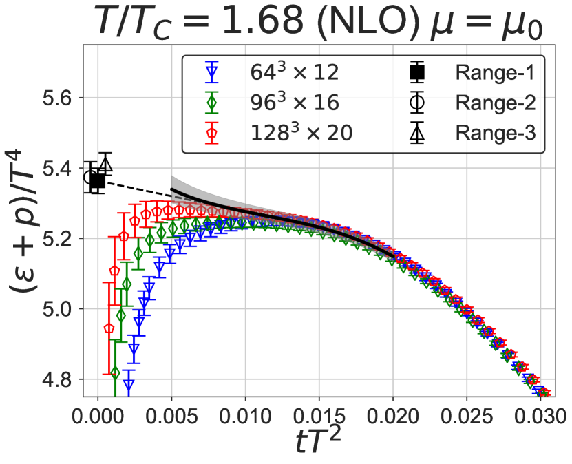
(a)

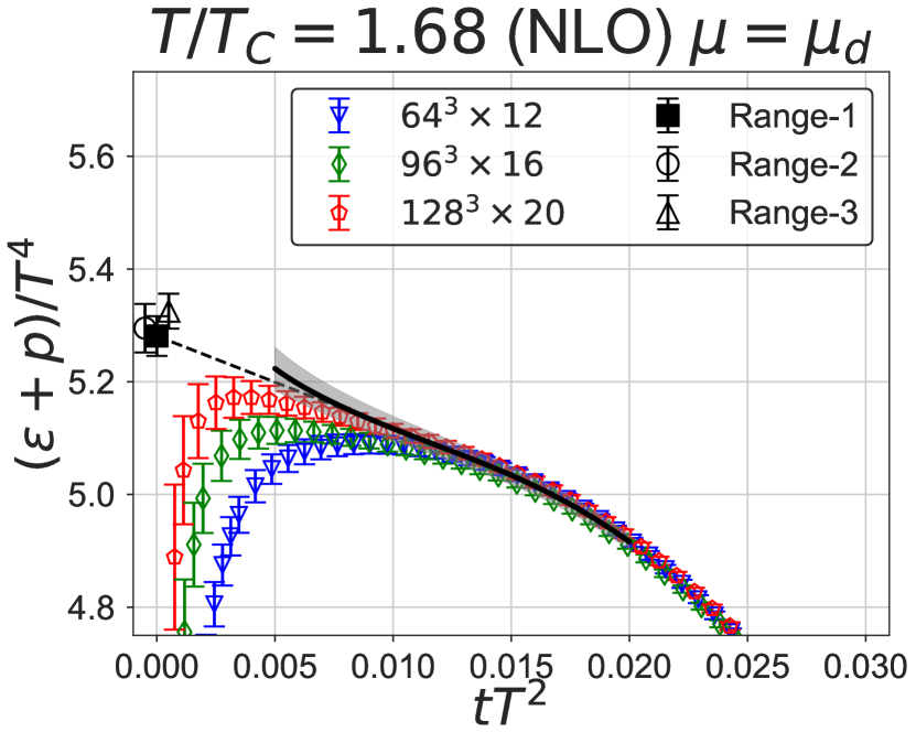
(b)

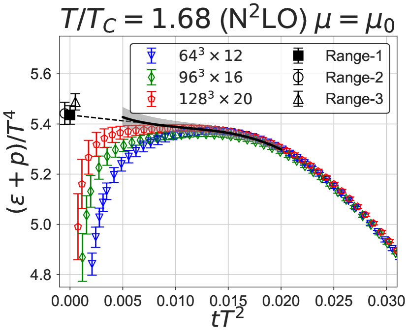
(c)

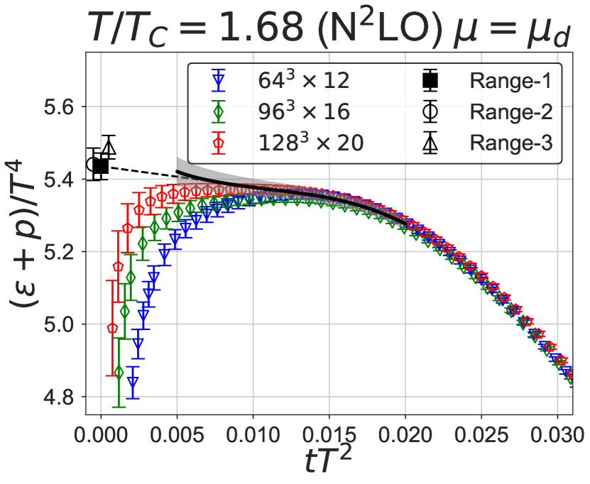
(d)

Figure 1: Equation (3.1) as a function of $tT^{2}$ for $T/T_{c}=1.68$. In each panel, the order of perturbation theory and the choice of the renormalization scale are indicated. The errors are statistical only. The extrapolation of the continuum limit (the gray band) to $t=0$ is plotted by the black circle (obtained by the fit range (3.2)), the white circle (obtained by the fit range (3.3)), and the white triangle (obtained by the fit range (3.4)).

We then take the continuum limit $a\to 0$ at each fixed value of $tT^{2}$. (See Ref. Kitazawa:2016dsl for details of this procedure.) The continuum limit results are shown by gray bands. In Fig. 1 and in the corresponding figures in Appendix A, Figs. 5–11, we observe that the use of the two-loop order coefficient generally reduces the $t$ dependence of the continuum limit (it becomes flatter in $t$). This behavior generally allows us to perform stable $t\to 0$ extrapolation.

We carry out the $t\to 0$ extrapolation with a linear function in $t$ as Ref. Kitazawa:2016dsl . The following three reasonable fit ranges are adopted for the $t\to 0$ extrapolation Kitazawa:2016dsl :

$$\text{Range~{}1: $0.01\leq tT^{2}\leq 0.015$},$$ (3.2)

$$\text{Range~{}2: $0.005\leq tT^{2}\leq 0.015$},$$ (3.3)

$$\text{Range~{}3: $0.01\leq tT^{2}\leq 0.02$}.$$ (3.4)

In Table 1, the coefficients of the linear term in $t$, determined in $t\to 0$ extrapolation using Range 1, are shown. The tendency for the slopes to get smaller at $\text{N}^{2}\text{LO}$ than at NLO is quantitatively observed. In addition to the linear function in $t$, we also use the linear function of $[g(\mu)^{2}/(4\pi)^{2}]^{\ell+1}$, where $\ell=1$ for the NLO approximation and $\ell=2$ for the $\text{N}^{2}\text{LO}$ approximation. This functional form is suggested from a detailed study of the asymptotic behavior of Eq. (3.1) for $t\to 0$ (H. Suzuki and H. Takaura, manuscript in preparation). We estimate the systematic error associated with the $t\to 0$ extrapolation by examining the variation obtained from the different extrapolation function. As mentioned, the use of the two-loop coefficient leads to a flatter behavior with respect to $t$. Hence, $t\to 0$ extrapolation becomes less sensitive to the fit function, the fit range, and the choice of the renormalization scale.

$(\varepsilon+p)/T^{4}$
$T/T_{c}$	NLO	$\text{N}^{2}\text{LO}$
0.93	$0.6(1.5)$	$0.8(1.6)$
1.02	$-5.6(1.7)$	$-2.0(1.7)$
1.12	$-5.0(1.9)$	$0.3(1.9)$
1.40	$-4.7(1.6)$	$0.2(1.7)$
1.68	$-8.7(1.6)$	$-4.7(1.7)$
2.10	$-5.5(1.5)$	$-2.2(1.6)$
2.31	$-2.4(2.4)$	$0.7(2.4)$
2.69	$-7.0(1.5)$	$-4.4(1.5)$
$(\varepsilon-3p)/T^{4}$
$T/T_{c}$	$\text{N}^{2}\text{LO}$	$\text{N}^{3}\text{LO}$
0.93	$1.3(1.1)$	$1.2(1.1)$
1.02	$1.9(1.0)$	$0.6(1.0)$
1.12	$2.5(1.0)$	$1.0(1.0)$
1.40	$0.8(1.0)$	$0.1(1.0)$
1.68	$-0.9(0.7)$	$-1.3(0.7)$

Table 1: Linear coefficients in the $t\to 0$ extrapolation. The renormalization scale $\mu_{0}(t)$ and Range 1 are used.

$(\varepsilon+p)/T^{4}$
$T/T_{c}$	NLO	$\text{N}^{2}\text{LO}$	FlowQCD 2016
0.93	$0.082(34)(02)(01)(00)(05)$	$0.083(35)(02)(01)(00)(01)$	0.082(33)(${}^{+3}_{-6}$)(0)
1.02	$2.128(64)(09)(25)(25)(57)$	$2.163(66)(09)(25)(04)(06)$	2.104(63)(${}^{+16}_{-2}$)(8)
1.12	$3.651(47)(32)(41)(50)(60)$	$3.709(49)(34)(41)(05)(01)$	3.603(46)(${}^{+39}_{-0}$)(13)
1.40	$4.777(36)(49)(51)(74)(72)$	$4.847(37)(53)(51)(01)(01)$	4.706(35)(${}^{+49}_{-0}$)(17)
1.68	$5.363(36)(48)(54)(82)(158)$	$5.436(37)(52)(54)(01)(37)$	5.285(35)(${}^{+44}_{-0}$)(18)
2.10	$5.694(35)(71)(54)(80)(117)$	$5.762(35)(75)(53)(01)(22)$	5.617(34)(${}^{+66}_{-0}$)(18)
2.31	$5.731(56)(87)(53)(77)(55)$	$5.797(56)(92)(52)(01)(08)$	5.657(55)(${}^{+82}_{-15}$)(18)
2.69	$5.986(33)(75)(52)(75)(175)$	$6.050(33)(80)(52)(02)(55)$	5.914(32)(${}^{+70}_{-0}$)(18)
$(\varepsilon-3p)/T^{4}$
$T/T_{c}$	$\text{N}^{2}\text{LO}$	$\text{N}^{3}\text{LO}$	FlowQCD 2016
0.93	$0.066(32)(03)(00)(00)(12)$	$0.066(32)(03)(00)(00)(02)$	0.066(32)(${}^{+3}_{-2}$)(0)
1.02	$1.947(58)(07)(00)(03)(20)$	$1.934(57)(07)(00)(03)(02)$	1.945(57)(${}^{+8}_{-7}$)(0)
1.12	$2.564(33)(11)(00)(04)(29)$	$2.548(33)(11)(01)(01)(04)$	2.560(33)(${}^{+12}_{-8}$)(0)
1.40	$1.779(24)(14)(00)(03)(12)$	$1.769(24)(14)(00)(01)(01)$	1.777(24)(${}^{+14}_{-3}$)(0)
1.68	$1.203(19)(10)(00)(02)(17)$	$1.196(18)(10)(00)(01)(10)$	1.201(19)(${}^{+10}_{-0}$)(0)

Table 2: Summary of the entropy density and the trace anomaly obtained by using coefficients in different orders of perturbation theory. The statistical errors are shown in the first parentheses. The numbers in the other parentheses show systematic errors: the error associated with the fit range, the $3\%$ uncertainty of $\Lambda_{\overline{\text{MS}}}$, the renormalization scale, and the $t\to 0$ extrapolation function are shown in the second, third, fourth, and fifth parentheses, respectively. The results of Ref. Kitazawa:2016dsl (FlowQCD 2016) are also tabulated in the last column: the numbers in the first, second, and third parentheses are the statistical error, the systematic error associated with the choice of the fit range (only the linear $t$ fit is adopted in Ref. Kitazawa:2016dsl ), and the systematic error associated with $\Lambda_{\overline{\text{MS}}}$ (varying it by $1\%$ in Ref. Kitazawa:2016dsl ). (The difference in the central values between FlowQCD 2016 and our analyses at the lower orders stems from the choice of the renormalization scale; $\mu_{0}(t)$ is adopted in the present work rather than $\mu_{d}(t)$).

In Table 2, the result of $(\epsilon+p)/T^{4}$ is summarized. The central values and the statistical errors are obtained by the linear $t$ fit in Range 1 (3.2) with the choice of the renormalization scale $\mu=\mu_{0}(t)$ (2.10). The systematic errors associated with (i) the fit range (estimated by other choices, Range 2 (3.3) and Range 3 (3.4)), (ii) the uncertainty of $\Lambda_{\overline{\text{MS}}}$ of $3\%$ Aoki:2016frl , (iii) the renormalization scale (estimated from another choice $\mu=\mu_{d}(t)$ (2.9)), and (iv) the $t\to 0$ extrapolation (estimated by adopting a different extrapolation function) are shown. Because of the reduction of the $t$ dependence with the two-loop coefficient, one can see that the systematic errors associated with the choice of the renormalization scale and the fit function are greatly reduced in the $\text{N}^{2}\text{LO}$ approximation. This clearly shows an advantage of the two-loop order coefficient.

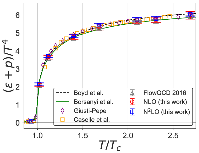
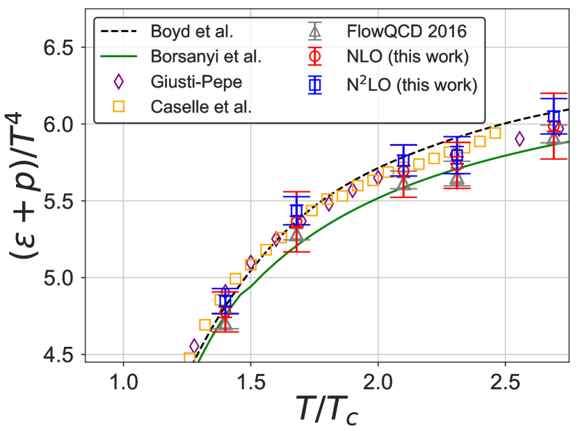
Figure 2: Summary of the entropy density $(\varepsilon+p)/T^{4}$ as a function of $T/T_{c}$. In the right-hand panel, the region $4.5\lesssim(\varepsilon+p)/T^{4}\lesssim 6.5$ is magnified. The results from the present paper are the red circles (NLO) and the blue squares ($\text{N}^{2}\text{LO}$). The error bars include the systematic error as well as the statistical error; see Table 2 and the main text for details. For comparison, we also show the results of Refs. Boyd:1996bx ; Borsanyi:2012ve ; Giusti:2016iqr ; Caselle:2018kap ; Kitazawa:2016dsl .

In Fig. 2, $(\epsilon+p)/T^{4}$ is plotted as a function of $T/T_{c}$. The error bar represents the total error, obtained by combining all the errors in quadrature. Our $\text{N}^{2}\text{LO}$ results are consistent with the results of Refs. Boyd:1996bx ; Borsanyi:2012ve ; Giusti:2016iqr ; Caselle:2018kap ; Kitazawa:2016dsl , especially with Refs. Boyd:1996bx ; Caselle:2018kap .

Reference Kitazawa:2016dsl is the preceding analysis performed with the same method as this work but with the NLO coefficient. In our NLO analysis, the systematic errors are investigated in more detail, including some additional error sources. This leads to larger errors than in Ref. Kitazawa:2016dsl , while the central values of Ref. Kitazawa:2016dsl are consistent with the present work. Figure 2 clearly shows that the use of the two-loop coefficient generally reduces the systematic errors.

We now turn to the trace anomaly, $\varepsilon-3p$, which is investigated in a parallel manner to the entropy density. The expectation value

$$-\frac{4}{T^{4}}c_{2}(t)\left\langle G_{\mu\nu}^{a}(t,x)G_{\mu\nu}^{a}(t,x)\right\rangle,$$ (3.5)

as a function of $tT^{2}$ is plotted in Fig. 3 for $T/T_{c}=1.68$. (Results for other temperatures are deferred to Appendix A.) As we noted, the two-loop order ($\text{N}^{2}\text{LO}$) and the three-loop order ($\text{N}^{3}\text{LO}$) coefficients are available for the trace anomaly. We observe that already with the $\text{N}^{2}\text{LO}$ coefficient the continuum limit (the gray band) is almost constant in $t$ within our fit ranges. Thus, naturally, the extrapolation of the continuum limit to $t=0$ is quite insensitive to the choices $\text{N}^{2}\text{LO}$ or $\text{N}^{3}\text{LO}$, and $\mu=\mu_{0}(t)$ or $\mu=\mu_{d}(t)$. Similarly to the entropy density above, we use the linear function of $t$ for the $t\to 0$ extrapolation. We also use the linear function of $[g(\mu)^{2}/(4\pi)^{2}]^{\ell}$, where $\ell=2$ for the $\text{N}^{2}\text{LO}$ approximation and $\ell=3$ for the $\text{N}^{3}\text{LO}$ approximation, as suggested from the study of the asymptotic $t\to 0$ behavior of Eq. (3.5) (H. Suzuki and H. Takaura, manuscript in preparation). The difference caused by this is treated as a systematic error. The results are summarized in Table 2 and Fig. 4. All the results are almost degenerate as seen from Fig. 4. However, it is worth noting that the use of the $\text{N}^{3}\text{LO}$ coefficient certainly reduces the dependences on the choice of the renormalization scale and the fit function, as seen from the fourth and the fifth parentheses in Table 2.

(a)

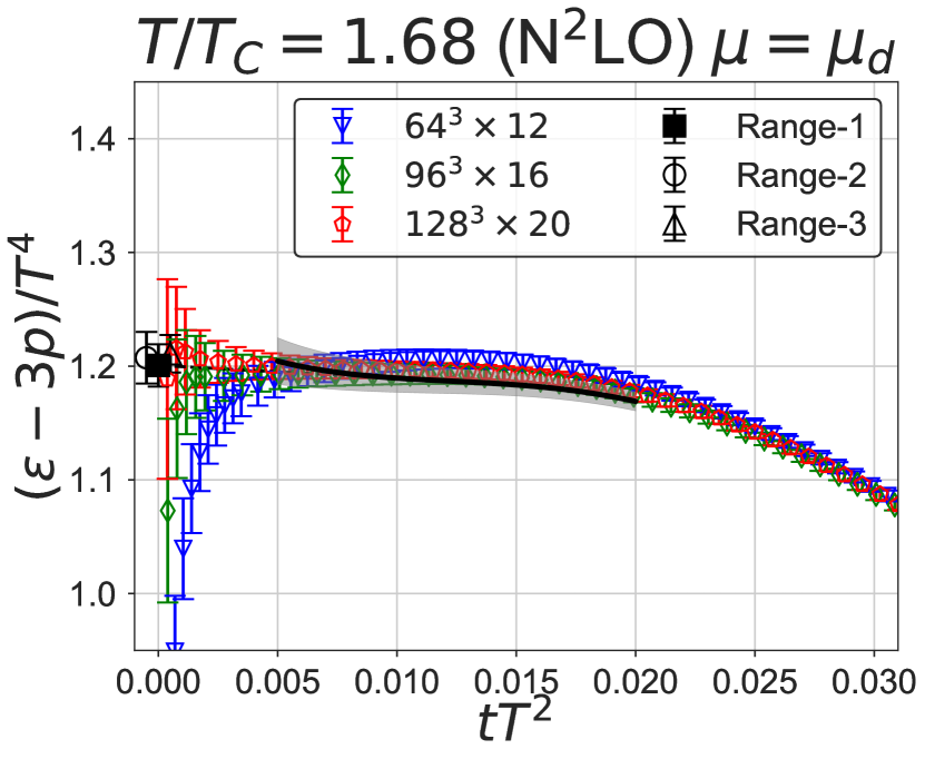
(b)

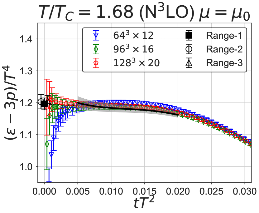
(c)

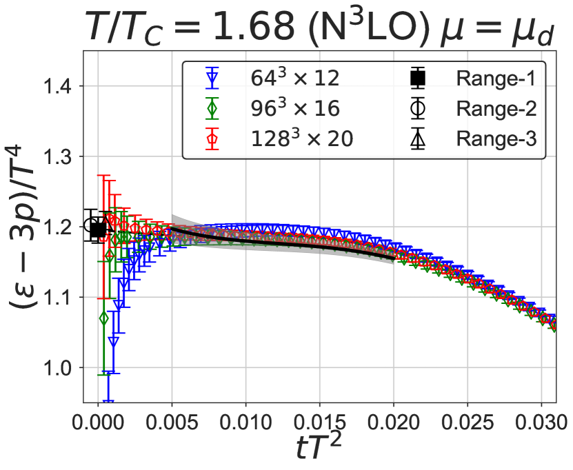
(d)

Figure 3: Equation (3.2) as a function of $tT^{2}$ for $T/T_{c}=1.68$. In each panel, the order of perturbation theory and the choice of the renormalization scale are indicated. The errors are statistical only. The extrapolation of the continuum limit (the gray band) to $t=0$ is plotted by the black circle (obtained by the fit range (3.2)), the white circle (obtained by the fit range (3.3)), and the white triangle (obtained by the fit range (3.4)).

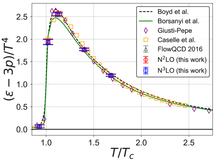
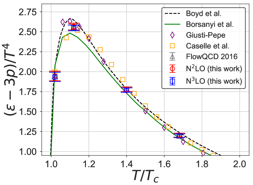
Figure 4: Summary of the trace anomaly $(\varepsilon-3p)/T^{4}$ as a function of $T/T_{c}$. In the right-hand panel, the region $1.00\lesssim(\varepsilon-3p)/T^{4}\lesssim 2.75$ is magnified. The results from the present paper are the red circles ($\text{N}^{2}\text{LO}$) and the blue squares ($\text{N}^{3}\text{LO}$). The error bars include the systematic error as well as the statistical error; see Table 2 for details. For comparison, we also show the results of Refs. Boyd:1996bx ; Borsanyi:2012ve ; Giusti:2016iqr ; Caselle:2018kap ; Kitazawa:2016dsl .

4 Conclusions

We investigated the thermodynamics in quenched QCD using the gradient-flow representation of the EMT. In particular, we studied the effect of the $\text{N}^{2}\text{LO}$ coefficients in the gradient-flow formalism, which have become available recently. For the trace anomaly, we used the $\text{N}^{3}\text{LO}$ coefficient, which was obtained in this paper for quenched QCD. It turned out that the use of the $\text{N}^{2}\text{LO}$ (or $\text{N}^{3}\text{LO}$) coefficients considerably reduces the systematic errors, especially concerning the choice of the renormalization scale and the $t\to 0$ extrapolation. We expect that the use of the $\text{N}^{2}\text{LO}$ coefficients will also make precise studies possible in full QCD, which has been investigated with the NLO coefficients so far.

Appendix A Numerical results (continued)

In this appendix, we show the plots of Eqs. (3.1) and (3.2) for temperatures other than $T/T_{c}=1.68$ in Figs. 5–15.

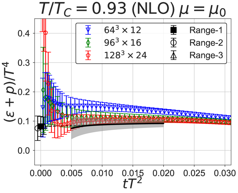
(a)

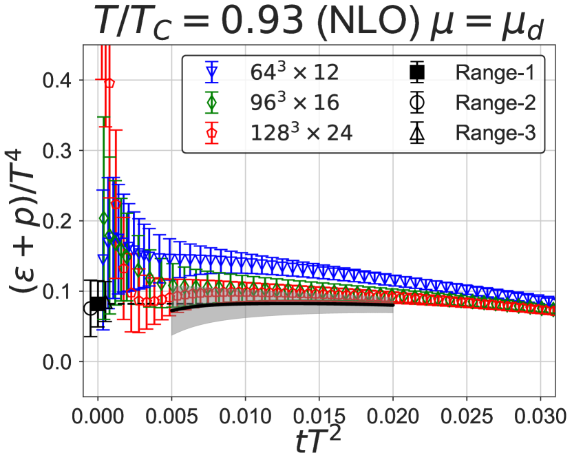
(b)

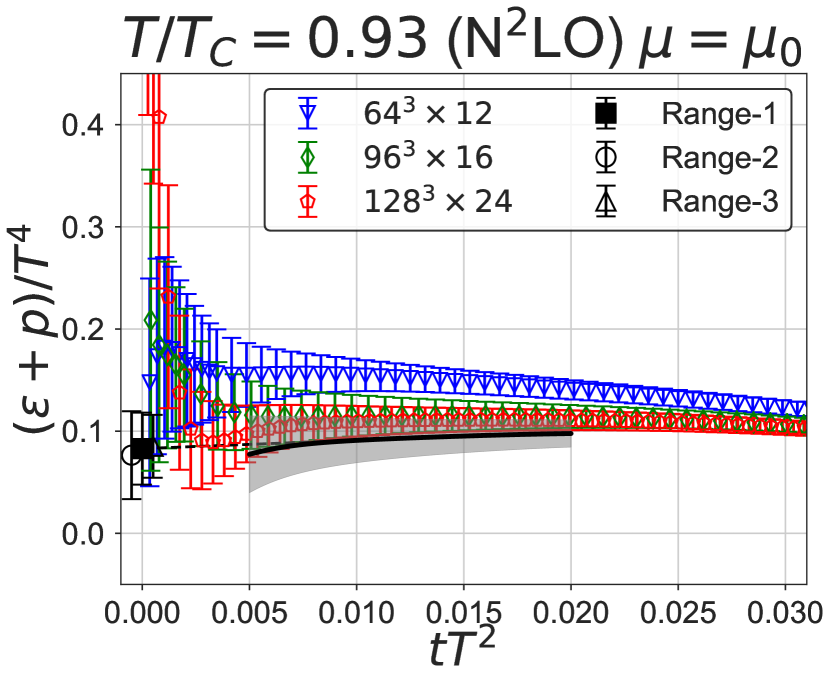
(c)

(d)

Figure 5: Same as Fig. 1. $T/T_{c}=0.93$.

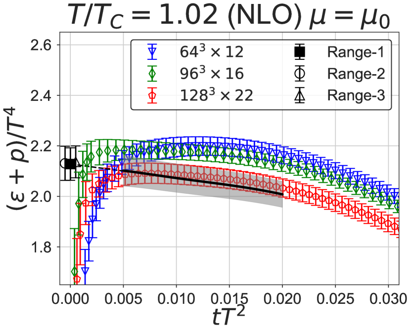
(a)

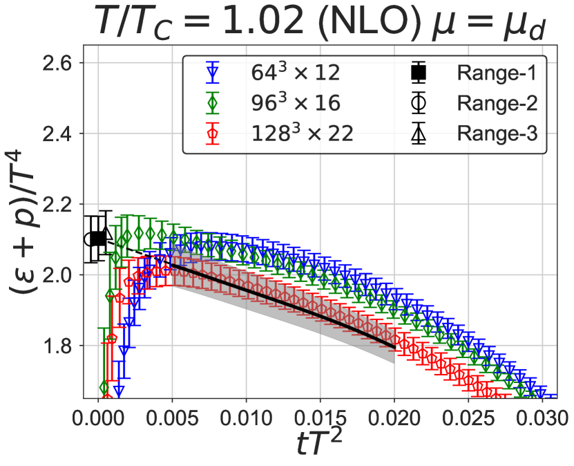
(b)

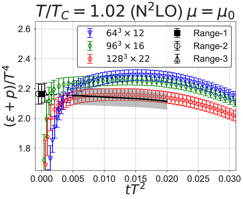
(c)

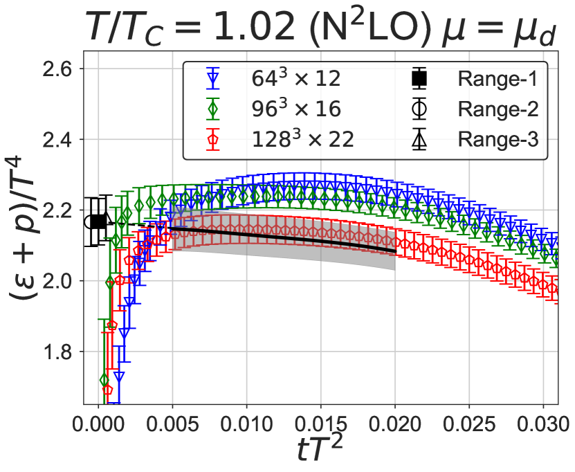
(d)

Figure 6: Same as Fig. 1. $T/T_{c}=1.02$.

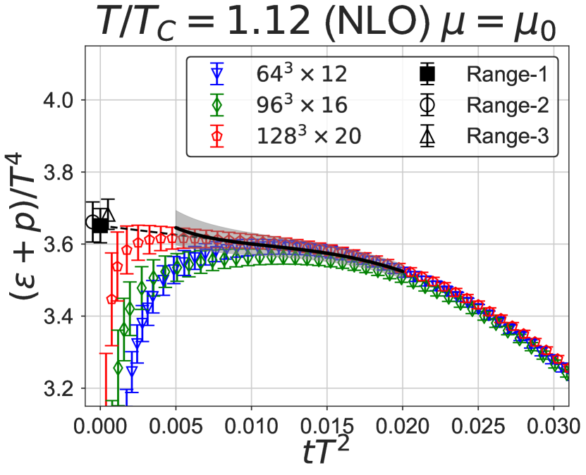
(a)

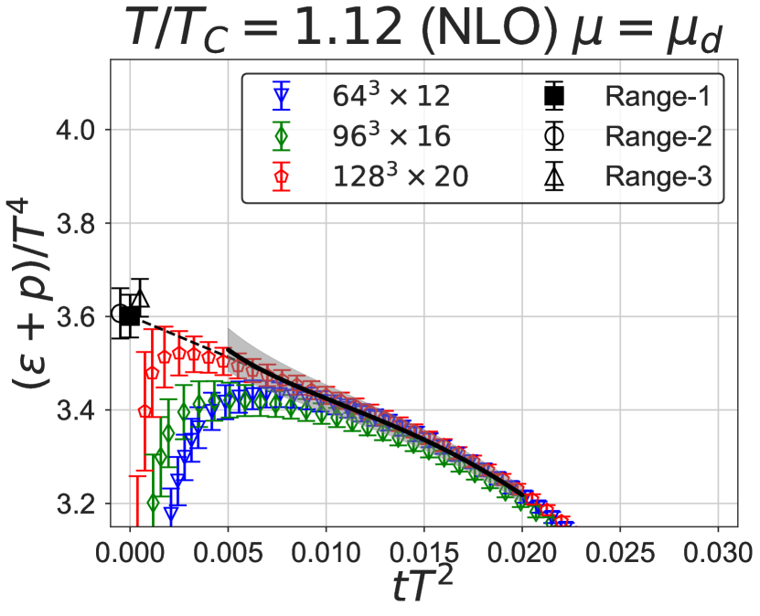
(b)

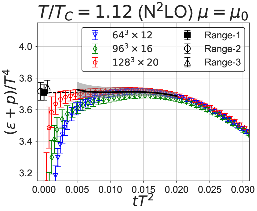
(c)

(d)

Figure 7: Same as Fig. 1. $T/T_{c}=1.12$.

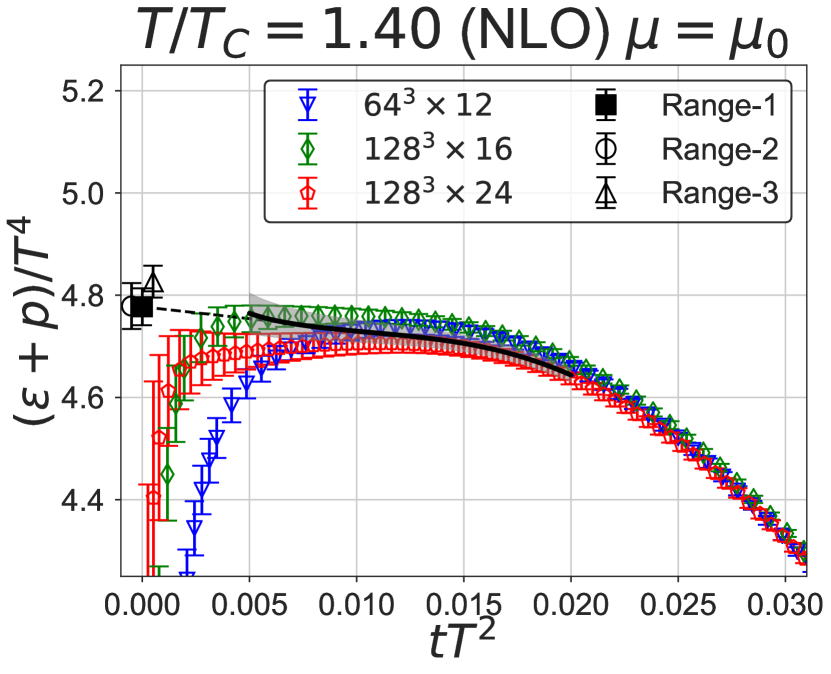
(a)

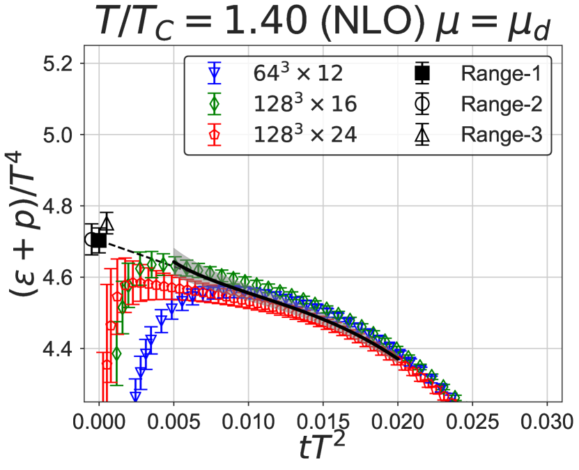
(b)

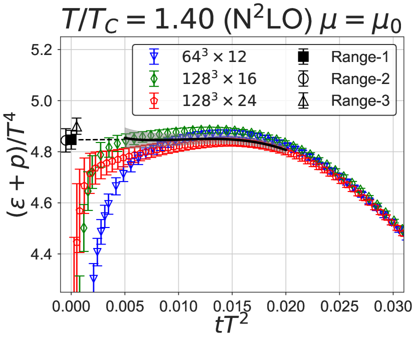
(c)

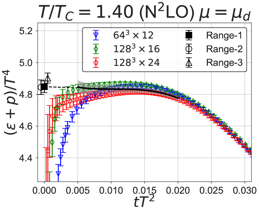
(d)

Figure 8: Same as Fig. 1. $T/T_{c}=1.40$.

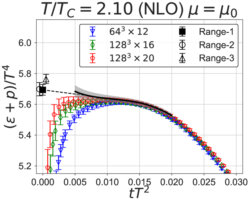
(a)

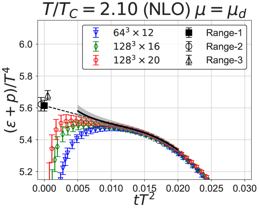
(b)

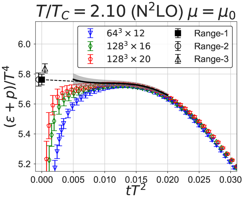
(c)

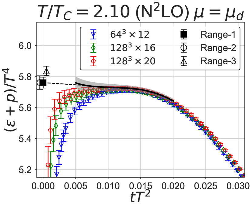
(d)

Figure 9: Same as Fig. 1. $T/T_{c}=2.10$.

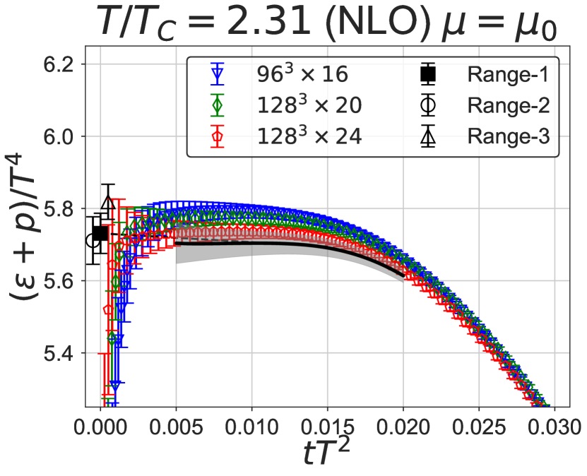
(a)

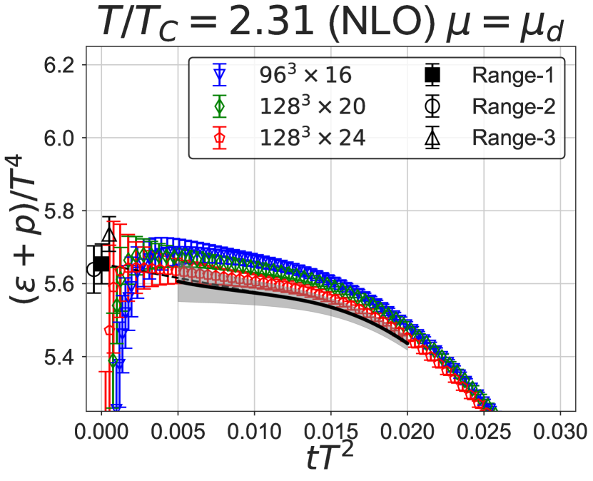
(b)

(c)

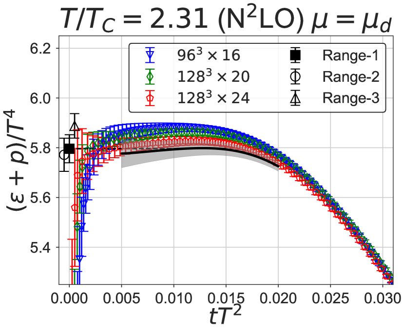
(d)

Figure 10: Same as Fig. 1. $T/T_{c}=2.31$.

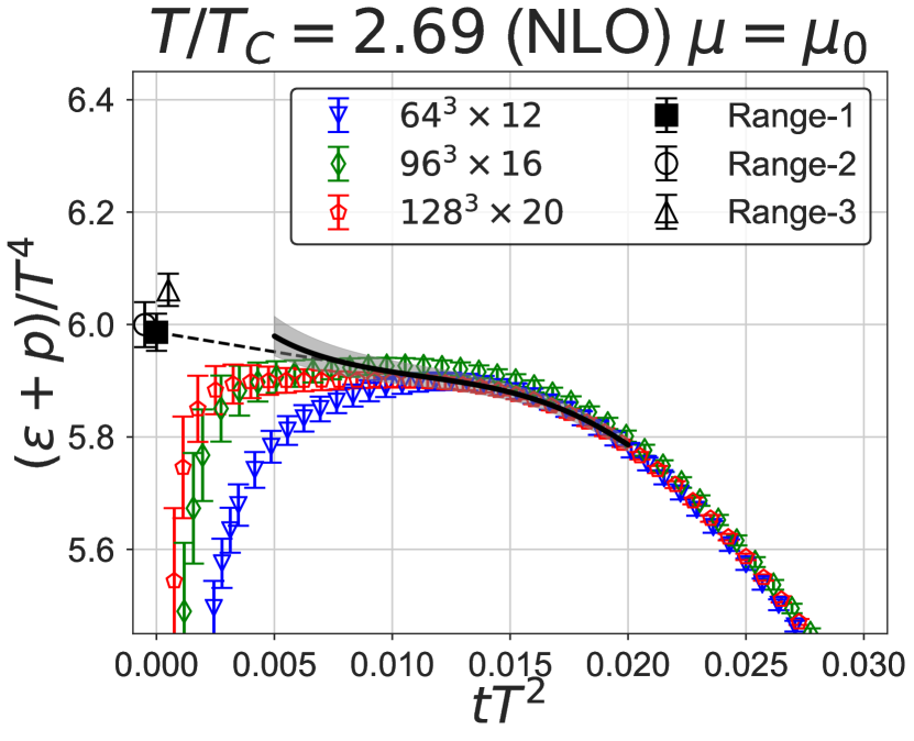
(a)

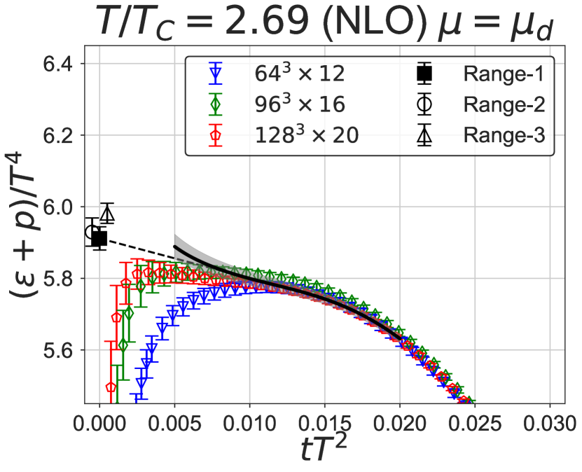
(b)

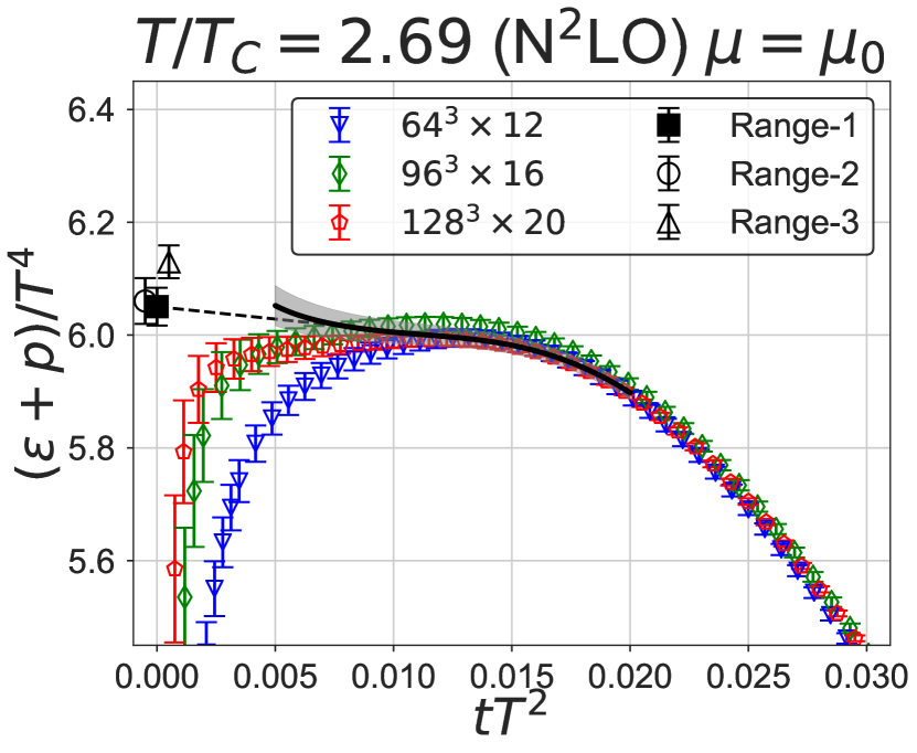
(c)

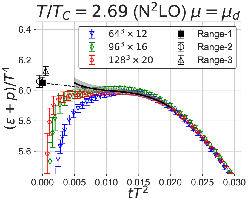
(d)

Figure 11: Same as Fig. 1. $T/T_{c}=2.69$.

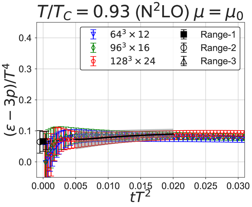
(a)

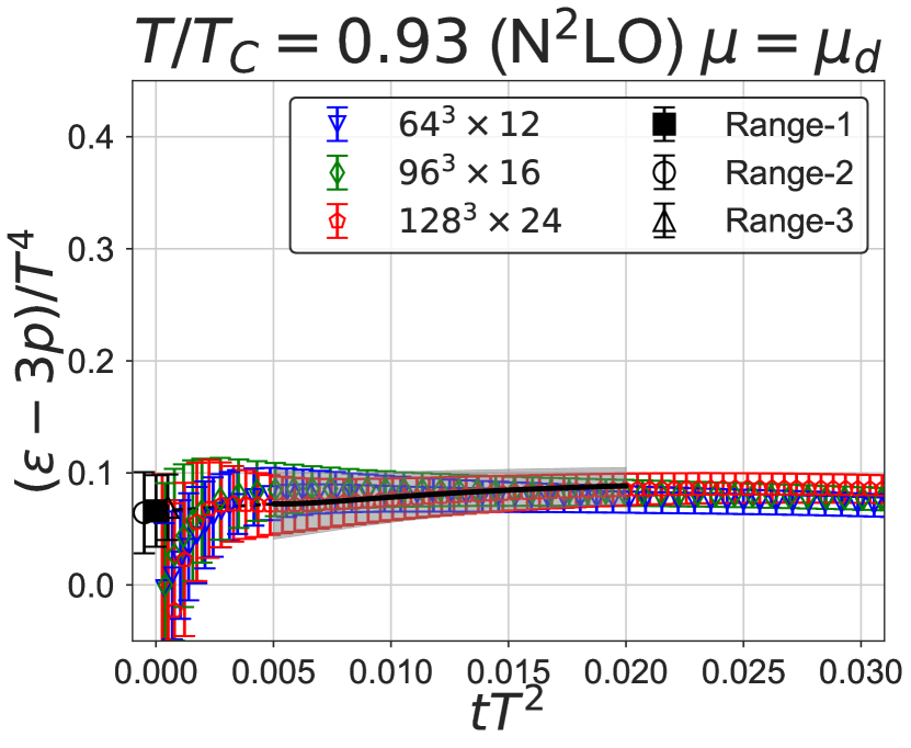
(b)

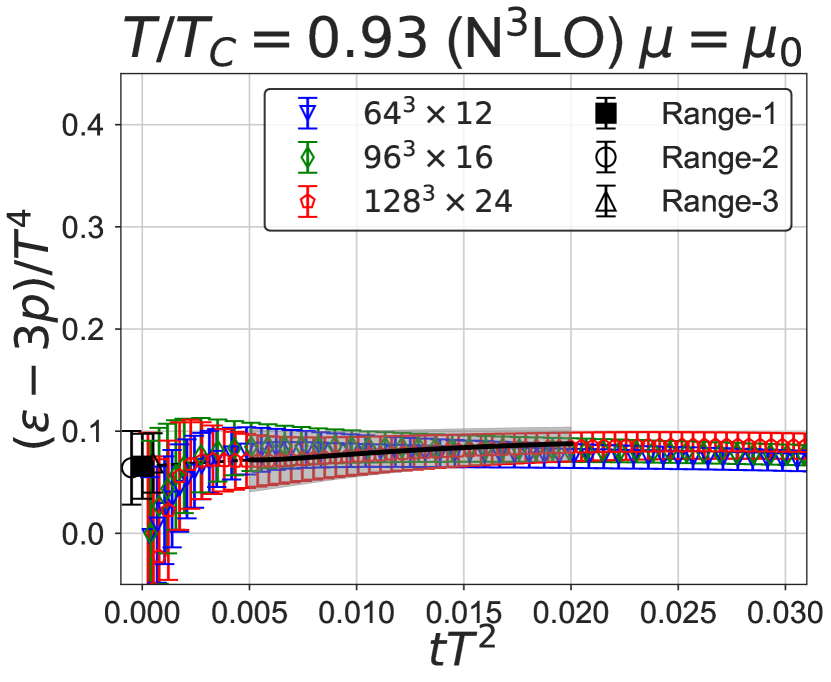
(c)

(d)

Figure 12: Same as Fig. 3. $T/T_{c}=0.93$.

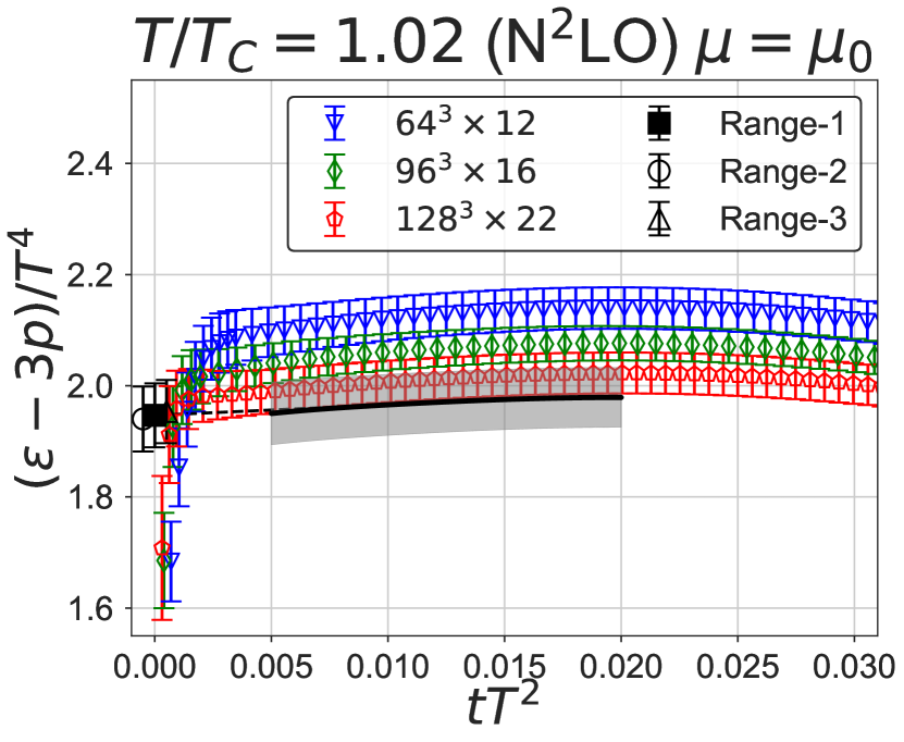
(a)

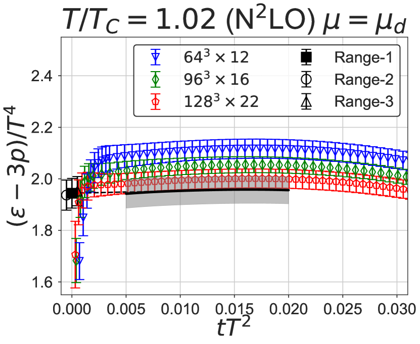
(b)

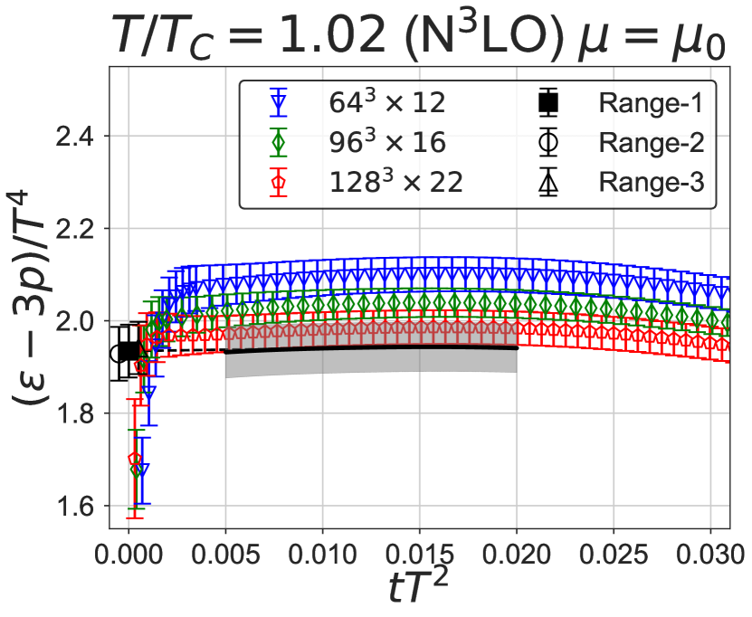
(c)

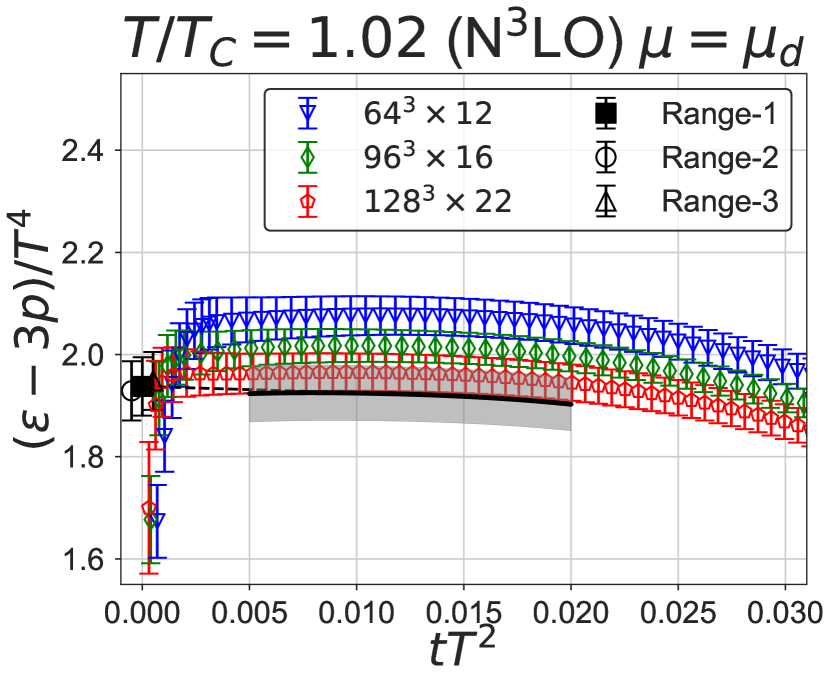
(d)

Figure 13: Same as Fig. 3. $T/T_{c}=1.02$.

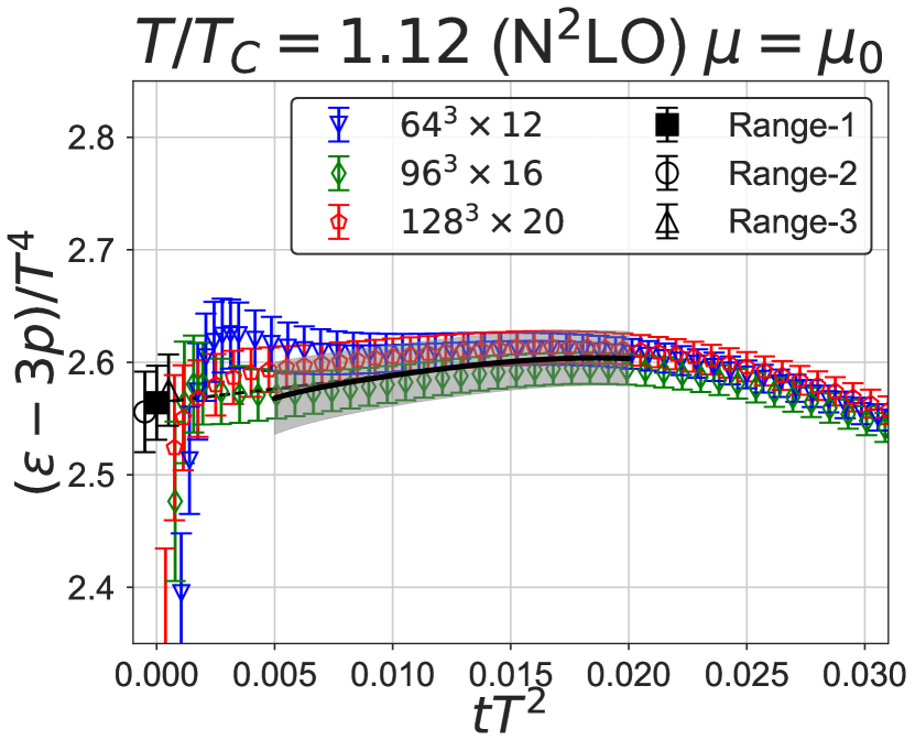
(a)

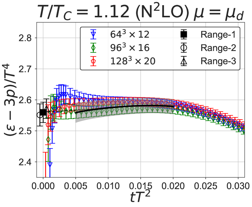
(b)

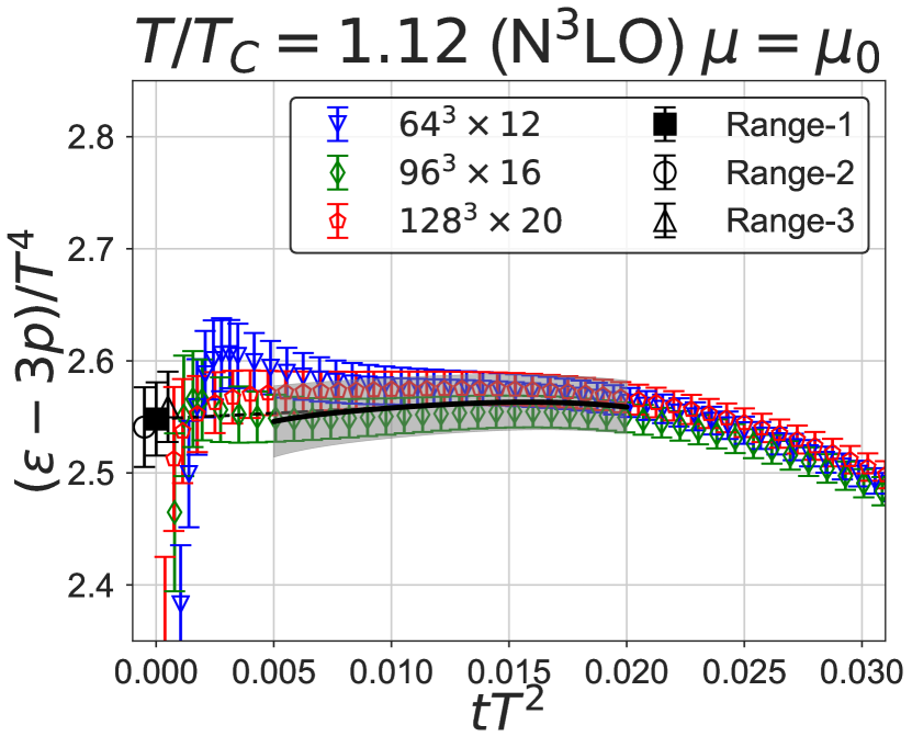
(c)

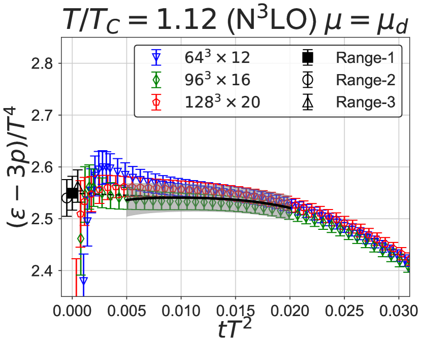
(d)

Figure 14: Same as Fig. 3. $T/T_{c}=1.12$.

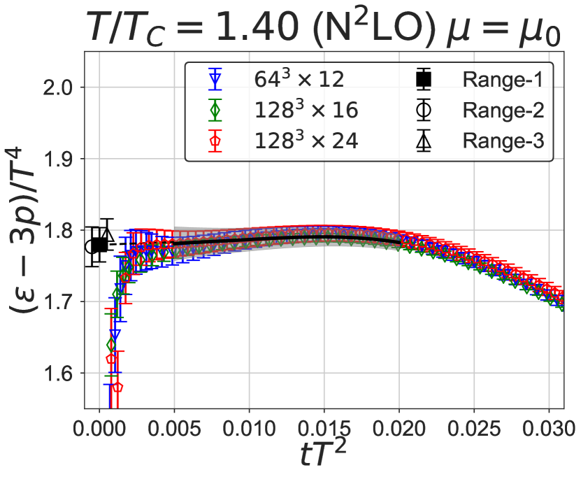
(a)

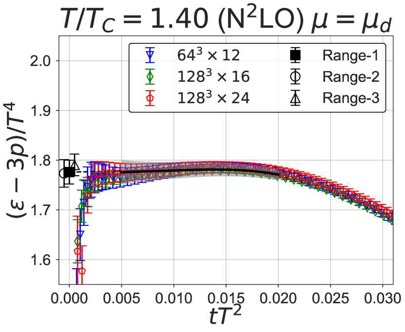
(b)

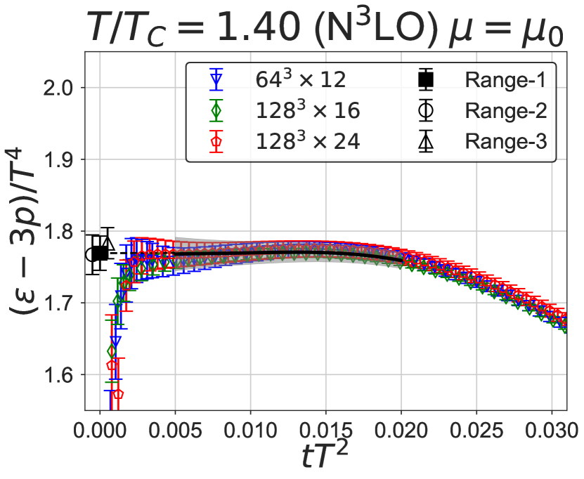
(c)

(d)

Figure 15: Same as Fig. 3. $T/T_{c}=1.40$.

References

- (1) H. Suzuki, PTEP 2013, 083B03 (2013) Erratum: [PTEP 2015, 079201 (2015)] doi:10.1093/ptep/ptt059, 10.1093/ptep/ptv094 [arXiv:1304.0533 [hep-lat]].
- (2) H. Makino and H. Suzuki, PTEP 2014, 063B02 (2014) Erratum: [PTEP 2015, 079202 (2015)] doi:10.1093/ptep/ptu070, 10.1093/ptep/ptv095 [arXiv:1403.4772 [hep-lat]].
- (3) R. Narayanan and H. Neuberger, JHEP 0603, 064 (2006) doi:10.1088/1126-6708/2006/03/064 [hep-th/0601210].
- (4) M. Lüscher, Commun. Math. Phys. 293, 899 (2010) doi:10.1007/s00220-009-0953-7 [arXiv:0907.5491 [hep-lat]].
- (5) M. Lüscher, JHEP 1008, 071 (2010) Erratum: [JHEP 1403, 092 (2014)] doi:10.1007/JHEP08(2010)071, 10.1007/JHEP03(2014)092 [arXiv:1006.4518 [hep-lat]].
- (6) M. Lüscher and P. Weisz, JHEP 1102, 051 (2011) doi:10.1007/JHEP02(2011)051 [arXiv:1101.0963 [hep-th]].
- (7) M. Lüscher, JHEP 1304, 123 (2013) doi:10.1007/JHEP04(2013)123 [arXiv:1302.5246 [hep-lat]].
- (8) S. Caracciolo, G. Curci, P. Menotti and A. Pelissetto, Annals Phys. 197, 119 (1990). doi:10.1016/0003-4916(90)90203-Z
- (9) H. Suzuki, PoS LATTICE 2016, 002 (2017) doi:10.22323/1.256.0002 [arXiv:1612.00210 [hep-lat]].
- (10) L. Del Debbio, A. Patella and A. Rago, JHEP 1311, 212 (2013) doi:10.1007/JHEP11(2013)212 [arXiv:1306.1173 [hep-th]].
- (11) F. Capponi, A. Rago, L. Del Debbio, S. Ehret and R. Pellegrini, PoS LATTICE 2015, 306 (2016) doi:10.22323/1.251.0306 [arXiv:1512.02851 [hep-lat]].
- (12) M. Asakawa et al. [FlowQCD Collaboration], Phys. Rev. D 90, no. 1, 011501 (2014) Erratum: [Phys. Rev. D 92, no. 5, 059902 (2015)] doi:10.1103/PhysRevD.90.011501, 10.1103/PhysRevD.92.059902 [arXiv:1312.7492 [hep-lat]].
- (13) Y. Taniguchi, S. Ejiri, R. Iwami, K. Kanaya, M. Kitazawa, H. Suzuki, T. Umeda and N. Wakabayashi, Phys. Rev. D 96, no. 1, 014509 (2017) doi:10.1103/PhysRevD.96.014509 [arXiv:1609.01417 [hep-lat]].
- (14) M. Kitazawa, T. Iritani, M. Asakawa, T. Hatsuda and H. Suzuki, Phys. Rev. D 94, no. 11, 114512 (2016) doi:10.1103/PhysRevD.94.114512 [arXiv:1610.07810 [hep-lat]].
- (15) S. Ejiri et al., PoS LATTICE 2016, 058 (2017) doi:10.22323/1.256.0058 [arXiv:1701.08570 [hep-lat]].
- (16) M. Kitazawa, T. Iritani, M. Asakawa and T. Hatsuda, Phys. Rev. D 96, no. 11, 111502 (2017) doi:10.1103/PhysRevD.96.111502 [arXiv:1708.01415 [hep-lat]].
- (17) K. Kanaya et al. [WHOT-QCD Collaboration], EPJ Web Conf. 175, 07023 (2018) doi:10.1051/epjconf/201817507023 [arXiv:1710.10015 [hep-lat]].
- (18) Y. Taniguchi et al. [WHOT-QCD Collaboration], EPJ Web Conf. 175, 07013 (2018) doi:10.1051/epjconf/201817507013 [arXiv:1711.02262 [hep-lat]].
- (19) R. Yanagihara, T. Iritani, M. Kitazawa, M. Asakawa and T. Hatsuda, Phys. Lett. B 789, 210 (2019) doi:10.1016/j.physletb.2018.09.067 [arXiv:1803.05656 [hep-lat]].
- (20) T. Hirakida, E. Itou and H. Kouno, arXiv:1805.07106 [hep-lat].
- (21) M. Shirogane, S. Ejiri, R. Iwami, K. Kanaya, M. Kitazawa, H. Suzuki, Y. Taniguchi and T. Umeda, arXiv:1811.04220 [hep-lat].
- (22) G. Boyd, J. Engels, F. Karsch, E. Laermann, C. Legeland, M. Lütgemeier and B. Petersson, Nucl. Phys. B 469, 419 (1996) doi:10.1016/0550-3213(96)00170-8 [hep-lat/9602007].
- (23) M. Okamoto et al. [CP-PACS Collaboration], Phys. Rev. D 60, 094510 (1999) doi:10.1103/PhysRevD.60.094510 [hep-lat/9905005].
- (24) S. Borsányi, G. Endrődi, Z. Fodor, S. D. Katz and K. K. Szabó, JHEP 1207, 056 (2012) doi:10.1007/JHEP07(2012)056 [arXiv:1204.6184 [hep-lat]].
- (25) S. Borsányi, Z. Fodor, C. Hoelbling, S. D. Katz, S. Krieg and K. K. Szabó, Phys. Lett. B 730, 99 (2014) doi:10.1016/j.physletb.2014.01.007 [arXiv:1309.5258 [hep-lat]].
- (26) A. Bazavov et al. [HotQCD Collaboration], Phys. Rev. D 90, 094503 (2014) doi:10.1103/PhysRevD.90.094503 [arXiv:1407.6387 [hep-lat]].
- (27) M. Shirogane, S. Ejiri, R. Iwami, K. Kanaya and M. Kitazawa, Phys. Rev. D 94, no. 1, 014506 (2016) doi:10.1103/PhysRevD.94.014506 [arXiv:1605.02997 [hep-lat]].
- (28) L. Giusti and M. Pepe, Phys. Rev. Lett. 113, 031601 (2014) doi:10.1103/PhysRevLett.113.031601 [arXiv:1403.0360 [hep-lat]].
- (29) L. Giusti and M. Pepe, Phys. Rev. D 91, 114504 (2015) doi:10.1103/PhysRevD.91.114504 [arXiv:1503.07042 [hep-lat]].
- (30) L. Giusti and M. Pepe, Phys. Lett. B 769, 385 (2017) doi:10.1016/j.physletb.2017.04.001 [arXiv:1612.00265 [hep-lat]].
- (31) M. Dalla Brida, L. Giusti and M. Pepe, EPJ Web Conf. 175, 14012 (2018) doi:10.1051/epjconf/201817514012 [arXiv:1710.09219 [hep-lat]].
- (32) M. Caselle, A. Nada and M. Panero, Phys. Rev. D 98, no. 5, 054513 (2018) doi:10.1103/PhysRevD.98.054513 [arXiv:1801.03110 [hep-lat]].
- (33) J. Engels, F. Karsch and T. Scheideler, Nucl. Phys. B 564, 303 (2000) doi:10.1016/S0550-3213(99)00522-2 [hep-lat/9905002].
- (34) R. V. Harlander, Y. Kluth and F. Lange, Eur. Phys. J. C 78, no. 11, 944 (2018) doi:10.1140/epjc/s10052-018-6415-7 [arXiv:1808.09837 [hep-lat]].
- (35) H. Suzuki, PTEP 2015, no. 10, 103B03 (2015) doi:10.1093/ptep/ptv139 [arXiv:1507.02360 [hep-lat]].
- (36) R. V. Harlander and T. Neumann, JHEP 1606, 161 (2016) doi:10.1007/JHEP06(2016)161 [arXiv:1606.03756 [hep-ph]].
- (37) S. L. Adler, J. C. Collins and A. Duncan, Phys. Rev. D 15, 1712 (1977). doi:10.1103/PhysRevD.15.1712
- (38) N. K. Nielsen, Nucl. Phys. B 120, 212 (1977). doi:10.1016/0550-3213(77)90040-2
- (39) J. C. Collins, A. Duncan and S. D. Joglekar, Phys. Rev. D 16, 438 (1977). doi:10.1103/PhysRevD.16.438
- (40) D. J. Gross and F. Wilczek, Phys. Rev. Lett. 30, 1343 (1973). doi:10.1103/PhysRevLett.30.1343
- (41) H. D. Politzer, Phys. Rev. Lett. 30, 1346 (1973). doi:10.1103/PhysRevLett.30.1346
- (42) W. E. Caswell, Phys. Rev. Lett. 33, 244 (1974). doi:10.1103/PhysRevLett.33.244
- (43) D. R. T. Jones, Nucl. Phys. B 75, 531 (1974). doi:10.1016/0550-3213(74)90093-5
- (44) O. V. Tarasov, A. A. Vladimirov and A. Y. Zharkov, Phys. Lett. 93B, 429 (1980). doi:10.1016/0370-2693(80)90358-5
- (45) S. A. Larin and J. A. M. Vermaseren, Phys. Lett. B 303, 334 (1993) doi:10.1016/0370-2693(93)91441-O [hep-ph/9302208].
- (46) T. van Ritbergen, J. A. M. Vermaseren and S. A. Larin, Phys. Lett. B 400, 379 (1997) doi:10.1016/S0370-2693(97)00370-5 [hep-ph/9701390].
- (47) M. Tanabashi et al. [Particle Data Group], Phys. Rev. D 98, no. 3, 030001 (2018). doi:10.1103/PhysRevD.98.030001
- (48) S. Aoki et al., Eur. Phys. J. C 77, no. 2, 112 (2017) doi:10.1140/epjc/s10052-016-4509-7 [arXiv:1607.00299 [hep-lat]].