MPI/PhT/97–012
TTP97–11
hep-ph/9704222
April 1997

Mass Corrections to the Vector Current Correlator

Abstract

Three-loop QCD corrections to the vector current correlator are considered. The large momentum procedure is applied in order to evaluate mass corrections up to order $(m^{2}/q^{2})^{6}$. The inclusion of the first seven terms to the ratio $R=\sigma(e^{+}e^{-}\to\mbox{hadrons})/\sigma(e^{+}e^{-}\to\mu^{+}\mu^{-})$ leads to reliable predictions from the high energy region down to relatively close to threshold.

PACS numbers: 12.38.-t, 12.38.Bx, 13.65.+i, 13.85.Lg.

^aMax-Planck-Institut für Physik, Werner-Heisenberg-Institut,
D-80805 Munich, Germany
^bInstitute for Nuclear Research, Russian Academy of Sciences,
Moscow 117312, Russia
^cInstitut für Theoretische Teilchenphysik, Universität Karlsruhe,
D-76128 Karlsruhe, Germany.

1 Introduction

One of the most precise measurements of the strong coupling constant $\alpha_{s}$ is provided by the decay rate $\Gamma(Z\to\mbox{hadrons})$. In the high energy limit the quark masses may often be neglected. However, for precision measurements it is desirable to include also mass corrections of the form $(m^{2}/s)^{l}$ with $l=1,2,3,\ldots$. This is particularly valid if one wants to predict the total cross section for $e^{+}e^{-}$ into hadrons in an energy region where $s$ and $m^{2}$ are of comparable magnitude. In the massless limit corrections up to order $\alpha_{s}^{3}$ are known [1, 2]. Terms of order $\alpha_{s}^{2}m^{2}/s$, $\alpha_{s}^{3}m^{2}/s$ [3, 4] and $\alpha_{s}^{2}m^{4}/s^{2}$ [5] are also available at present, providing an acceptable approximation from the high energy region down to intermediate energy values. For the energy region closer to the production threshold terms of higher order in $m^{2}/s$ are necessary. In this paper a systematic approach is presented to compute these terms. For the moment the vector current correlator only is considered. The starting point is thereby the polarization function $\Pi(q^{2})$. With the method presented below we are able to evaluate the three-loop terms up to order $(m^{2}/q^{2})^{6}$ in an expansion of $\Pi(q^{2})$.

The polarization function $\Pi(q^{2})$ is defined through

$$\left(-g_{\mu\nu}q^{2}+q_{\mu}q_{\nu}\right)\,\Pi(q^{2}) = i\int dx\,e^{iqx}\langle 0|Tj_{\mu}(x)j_{\nu}(0)|0\rangle$$ (1)

and the physical observable $R(s)$ is related to $\Pi(q^{2})$ by

$$R(s) = 12\pi\,\mbox{Im}\,\Pi(q^{2}=s+i\epsilon).$$ (2)

It is convenient to write

$$\Pi(q^{2}) = \Pi^{(0)}(q^{2})+\frac{\alpha_{s}(\mu^{2})}{\pi}C_{F}\Pi^{(1)}(q^{2})+\left(\frac{\alpha_{s}(\mu^{2})}{\pi}\right)^{2}\Pi^{(2)}(q^{2})+\ldots\,\,,$$ (3)

$$\Pi^{(2)} = C_{F}^{2}\Pi_{A}^{(2)}+C_{A}C_{F}\Pi_{\it NA}^{(2)}+C_{F}Tn_{l}\Pi_{l}^{(2)}+C_{F}T\Pi_{F}^{(2)},$$ (4)

and similarly for $R(s)$. The colour factors ($C_{F}=(N_{c}^{2}-1)/(2N_{c})$ and $C_{A}=N_{c}$) correspond to the Casimir operators of the fundamental and adjoint representations, respectively. For the numerical evaluation we set $N_{c}=3$. The trace normalization of the fundamental representation is $T=1/2$. The number of light (massless) quark flavours is denoted by $n_{l}$. In Eq. (4) $\Pi_{A}^{(2)}$ is the abelian contribution (quenched QED!) and $\Pi_{\it NA}^{(2)}$ is the non-abelian part specific for QCD. There are two fermionic contributions arising from double-bubble diagrams: For $\Pi_{l}^{(2)}$ the quark in the inner loop is massless, the external massive, whereas for $\Pi_{F}^{(2)}$ both fermions have the same mass. The result for $R_{l}^{(2)}(s)$ is known analytically [6] and will serve as check. The case where the external current couples to massless quarks and these via gluons to massive ones is treated in [7] and will not be addressed here.

The outline of the paper is as follows: In Sect. 2 we will describe the procedure which allows the systematic expansion for $\Pi(q^{2})$ in analytic form for large external momentum and its implementation in a program. Sect. 3 contains the results separated according to the colour factors. In Sect. 4 the imaginary part of $\Pi(q^{2})$ is considered and compared to the result of a recent evaluation using semi-analytical methods [8]. Finally the conclusions are presented in Sect. 5.

2 Large momentum procedure

In this section the basic rules of the large momentum procedure are briefly described and their implementation in programs is considered.

The methods which allow the expansion of Feynman diagrams containing either large masses (hard mass procedure) or large external momenta (large momentum procedure) have been used extensively in the recent past [9]. At one- and two-loop level it is in general still possible to perform the diagrammatic expansion “by hand” and only evaluate the integrals with algebraic programs. However, at three loops this is almost impossible, in particular if one is interested in an expansion up to high orders in $m^{2}/s$.

Following [10] the prescriptions for the expansion of an unrenormalized propagator type Feynman diagram in its large external momentum read:

1. Generate all subdiagrams of the initial graph such that

   1. they contain both vertices through which the large momentum enters and leaves the initial graph

   2. they become one-particle-irreducible when the two vertices are identified.

2. Taylor-expand the integrand of these subdiagrams in all small masses and external momenta generated by removing lines from the initial diagram.

3. In the initial diagram, shrink the subdiagram to a point and insert the result obtained from the expansion in 2.

4. Sum over all terms.

The subgraphs from step 1 are denoted hard subgraphs or simply subgraphs, the reduced graphs, resulting from step 3, the co-subgraphs.

Figure 1: Possible topologies for the subgraphs of an NO-type diagram.

For the non-planar three-loop topology all hard subgraphs are shown in Fig. 1. The corresponding co-subgraphs are obtained from the full graph by shrinking the displayed lines to a point. The number of terms generated by the large momentum procedure increases rapidly with the number of loops in the initial diagram. Also, the relation between the expansion momenta in the subgraph and the loop momenta of the co-subgraph becomes non-trivial. Nevertheless, the rules listed above provide an algorithm well suited for the evaluation through a computer. Restricting to three-loop two-point functions with large external momentum and an arbitrary number of small masses, the procedure was implemented using the language PERL. The program can be divided into the following steps:

1. 1. Generation of the relevant subgraphs and the corresponding co-subgraphs including the determination of their topologies, and

   2. distribution of momenta in the subgraph and co-subgraph respecting the relations between them.

2. Calculation of these terms.

In step 1a, one only considers topologies, disregarding any properties of lines except their relative positions. Especially one neglects their momenta, masses, particle types, etc. For the representation of a diagram we label its vertices by integers and specify lines by their endpoints. A topology is thus described by the collection of its lines.

To generate the subdiagrams we first note that the full graph is always one of the hard subgraphs. The remaining ones are obtained by going through the following steps:

1. Remove any combination of lines from the initial diagram.

2. Remove the emerging isolated dots and binary vertices.

3. Relabel the remaining vertices by $\{1,\ldots,\#{\rm vertices}\}$ and build all permutations.

4. Compare with a table listing the basic one- and two-loop topologies, assign the proper topology if it matches one of the entries or, otherwise, discard the result.

If a subgraph passes the last step, the corresponding co-subgraph is evidently fixed and its topology is determined in a similar way by applying steps (ii)-(iv). The result of this procedure is a database containing all relevant sub- and co-subgraphs, including information about their topology. Note that no selection criteria related to line properties have been applied so far. Thus, up to this point the procedure is universal and for each topology this part of the program has to be run only once and for all.

In step 1b, the database resulting from 1a is specialized to a specific diagram, including masses and momenta. The direction of the momentum carried by a line is connected with the order of the labels representing this line. Furthermore, for each subgraph the small external momenta are routed in a way that they touch as few lines as possible. The output of step 1 is then the input for step 2, together with all the necessary administrative files like makefiles etc.

In step 2 the two FORM [11] packages MATAD and MINCER are used which were already available and have been applied to many different problems. MINCER [12] calculates massless three-loop propagator type integrals and therefore applies to the hard subgraphs. MATAD calculates massive tadpole diagrams up to three loops by using the corresponding recursion formulas obtained in [13] and is used for the co-subgraphs accordingly.

Allowing only for one internal mass scale $m$, the final result is then a power series in $m^{2}/q^{2}$, where $q$ is the (large) external momentum. The coefficient functions contain numerical constants together with $\ln^{i}(-q^{2}/m^{2})$ and $\ln^{j}(-q^{2}/\mu^{2})$ with $i\leq 3$ and $j\leq 2$, where $\mu$ is the renormalization scale.

3 Mass corrections to $\Pi(q^{2})$

With the method presented in the previous section the first seven terms of the expansion have been computed. For the three-loop case 18 initial diagrams have to be considered. Altogether 240 subdiagrams are produced when the large momentum procedure is applied. The corresponding numbers in the two- (one-) loop case are 2 (1) initial and 14 (3) subdiagrams. The high energy approximation for $\Pi(q^{2})$ reads in the $\overline{\mbox{MS}}$ scheme ($l_{qm}\equiv\ln(-q^{2}/\bar{m}^{2})$, $l_{q\mu}\equiv\ln(-q^{2}/\mu^{2})$):

$$\bar{\Pi}^{(0)} = {3\over 16\pi^{2}}\,\bigg{\{}{20\over 9}-{4\over 3}\,l_{q\mu}+8\,{\bar{m}^{2}\over q^{2}}+\left({\bar{m}^{2}\over q^{2}}\right)^{2}\,\left(4+8\,l_{qm}\right)$$ (5)

$$\mbox{}+\left({\bar{m}^{2}\over q^{2}}\right)^{3}\,\left(-{64\over 9}+{32\over 3}\,l_{qm}\right)+\left({\bar{m}^{2}\over q^{2}}\right)^{4}\,\left(-22+24\,l_{qm}\right)$$

$$\mbox{}+\left({\bar{m}^{2}\over q^{2}}\right)^{5}\,\left(-{992\over 15}+64\,l_{qm}\right)+\left({\bar{m}^{2}\over q^{2}}\right)^{6}\,\left(-{1852\over 9}+{560\over 3}\,l_{qm}\right)\bigg{\}}+\ldots\,\,,$$

$$\bar{\Pi}^{(1)} = {3\over 16\pi^{2}}\,\bigg{\{}{55\over 12}-4\,\zeta_{3}-l_{q\mu}+{\bar{m}^{2}\over q^{2}}\,\left(16-12\,l_{q\mu}\right)$$ (6)

$$\mbox{}+\left({\bar{m}^{2}\over q^{2}}\right)^{2}\,\bigg{[}{2\over 3}+16\,\zeta_{3}+22\,l_{qm}-24\,l_{qm}\,l_{q\mu}+12\,l_{qm}^{2}\bigg{]}$$

$$\mbox{}+\left({\bar{m}^{2}\over q^{2}}\right)^{3}\,\bigg{[}-{736\over 27}+{1184\over 27}\,l_{qm}+{200\over 9}\,l_{qm}^{2}+\left(48-48\,l_{qm}\right)\,l_{q\mu}\bigg{]}$$

$$\mbox{}+\left({\bar{m}^{2}\over q^{2}}\right)^{4}\,\bigg{[}-{40313\over 216}+{1199\over 9}\,l_{qm}+{229\over 3}\,l_{qm}^{2}+\left(168-144\,l_{qm}\right)\,l_{q\mu}\bigg{]}$$

$$\mbox{}+\left({\bar{m}^{2}\over q^{2}}\right)^{5}\,\bigg{[}-{2641601\over 3375}+{279196\over 675}\,l_{qm}+{12248\over 45}\,l_{qm}^{2}+\left(592-480\,l_{qm}\right)\,l_{q\mu}\bigg{]}$$

$$\mbox{}+\left({\bar{m}^{2}\over q^{2}}\right)^{6}\,\bigg{[}-{6117262\over 2025}+{184066\over 135}\,l_{qm}+{8992\over 9}\,l_{qm}^{2}$$

$$\mbox{\hskip 28.45274pt}+\left(2132-1680\,l_{qm}\right)\,l_{q\mu}\bigg{]}\bigg{\}}+\ldots\,\,,$$

$$\bar{\Pi}^{(2)}_{A} = {3\over 16\pi^{2}}\,\bigg{\{}-{143\over 72}-{37\over 6}\,\zeta_{3}+10\,\zeta_{5}+{1\over 8}\,l_{q\mu}$$ (7)

$$\mbox{}+{\bar{m}^{2}\over q^{2}}\,\bigg{[}{1667\over 24}-{5\over 3}\,\zeta_{3}-{70\over 3}\,\zeta_{5}-{51\over 2}\,l_{q\mu}+9\,l_{q\mu}^{2}\bigg{]}$$

$$\mbox{}+\left({\bar{m}^{2}\over q^{2}}\right)^{2}\,\bigg{[}{127\over 2}+96\,\zeta_{3}-48\,\zeta_{4}-20\,\zeta_{5}+8\,B_{4}+\left(36+24\,\zeta_{3}\right)\,l_{qm}+{33\over 2}\,l_{qm}^{2}$$

$$\mbox{\hskip 28.45274pt}+12\,l_{qm}^{3}+\left(31-48\,\zeta_{3}-33\,l_{qm}-36\,l_{qm}^{2}\right)\,l_{q\mu}+\left(-18+36\,l_{qm}\right)\,l_{q\mu}^{2}\bigg{]}$$

$$\mbox{}+\left({\bar{m}^{2}\over q^{2}}\right)^{3}\,\bigg{[}-{177163\over 2916}-13\,\zeta_{3}-64\,\zeta_{4}+{320\over 3}\,\zeta_{5}+{32\over 3}\,B_{4}$$

$$\mbox{\hskip 28.45274pt}+\left({9988\over 81}+{248\over 3}\,\zeta_{3}\right)\,l_{qm}+{239\over 3}\,l_{qm}^{2}+{2896\over 81}\,l_{qm}^{3}$$

$$\mbox{\hskip 28.45274pt}+\left({1750\over 9}-{410\over 3}\,l_{qm}-100\,l_{qm}^{2}\right)\,l_{q\mu}+\left(-144+108\,l_{qm}\right)\,l_{q\mu}^{2}\bigg{]}$$

$$\mbox{}+\left({\bar{m}^{2}\over q^{2}}\right)^{4}\,\bigg{[}-{12656479\over 15552}-{14293\over 54}\,\zeta_{3}-144\,\zeta_{4}+{880\over 3}\,\zeta_{5}+24\,B_{4}$$

$$\mbox{\hskip 28.45274pt}+\left({26783\over 108}+{826\over 3}\,\zeta_{3}\right)\,l_{qm}+{494059\over 1296}\,l_{qm}^{2}+{53701\over 324}\,l_{qm}^{3}$$

$$\mbox{\hskip 28.45274pt}+\left({48263\over 36}-{1765\over 3}\,l_{qm}-458\,l_{qm}^{2}\right)\,l_{q\mu}+\left(-612+432\,l_{qm}\right)\,l_{q\mu}^{2}\bigg{]}$$

$$\mbox{}+\left({\bar{m}^{2}\over q^{2}}\right)^{5}\,\bigg{[}-{539215192817\over 116640000}-{1056859\over 900}\,\zeta_{3}-384\,\zeta_{4}+{3200\over 3}\,\zeta_{5}+64\,B_{4}$$

$$\mbox{\hskip 28.45274pt}+\left({1191314219\over 3240000}+{14234\over 15}\,\zeta_{3}\right)\,l_{qm}+{90647953\over 54000}\,l_{qm}^{2}+{2940547\over 4050}\,l_{qm}^{3}$$

$$\mbox{\hskip 28.45274pt}+\left({328233\over 50}-{105554\over 45}\,l_{qm}-{6124\over 3}\,l_{qm}^{2}\right)\,l_{q\mu}+\left(-2580+1800\,l_{qm}\right)\,l_{q\mu}^{2}\bigg{]}$$

$$\mbox{}+\left({\bar{m}^{2}\over q^{2}}\right)^{6}\,\bigg{[}-{420607059143\over 19440000}-{13059229\over 2700}\,\zeta_{3}-1120\,\zeta_{4}+4000\,\zeta_{5}+{560\over 3}\,B_{4}$$

$$\mbox{\hskip 28.45274pt}+\left({133099291\over 972000}+{16842\over 5}\,\zeta_{3}\right)\,l_{qm}+{54076013\over 7200}\,l_{qm}^{2}+{8575579\over 2700}\,l_{qm}^{3}$$

$$\mbox{\hskip 28.45274pt}+\left({13274779\over 450}-{142256\over 15}\,l_{qm}-8992\,l_{qm}^{2}\right)\,l_{q\mu}$$

$$\mbox{\hskip 28.45274pt}+\left(-10854+7560\,l_{qm}\right)\,l_{q\mu}^{2}\bigg{]}\bigg{\}}+\ldots\,\,,$$

$$\bar{\Pi}^{(2)}_{\it NA} = {3\over 16\pi^{2}}\,\bigg{\{}{44215\over 2592}-{227\over 18}\,\zeta_{3}-{5\over 3}\,\zeta_{5}+\left(-{41\over 8}+{11\over 3}\,\zeta_{3}\right)\,l_{q\mu}+{11\over 24}\,l_{q\mu}^{2}$$ (8)

$$\mbox{}+{\bar{m}^{2}\over q^{2}}\,\bigg{[}{1447\over 24}+{16\over 3}\,\zeta_{3}-{85\over 3}\,\zeta_{5}-{185\over 6}\,l_{q\mu}+{11\over 2}\,l_{q\mu}^{2}\bigg{]}$$

$$\mbox{}+\left({\bar{m}^{2}\over q^{2}}\right)^{2}\,\bigg{[}-{5051\over 216}+{529\over 9}\,\zeta_{3}+24\,\zeta_{4}-30\,\zeta_{5}-4\,B_{4}+\left({2123\over 36}-12\,\zeta_{3}\right)\,l_{qm}$$

$$\mbox{\hskip 28.45274pt}+{76\over 3}\,l_{qm}^{2}+{11\over 3}\,l_{qm}^{3}+\left(-{11\over 18}-{44\over 3}\,\zeta_{3}-{105\over 2}\,l_{qm}-11\,l_{qm}^{2}\right)\,l_{q\mu}+11\,l_{qm}\,l_{q\mu}^{2}\bigg{]}$$

$$\mbox{}+\left({\bar{m}^{2}\over q^{2}}\right)^{3}\,\bigg{[}-{1278391\over 11664}+{149\over 2}\,\zeta_{3}+32\,\zeta_{4}-{80\over 3}\,\zeta_{5}-{16\over 3}\,B_{4}$$

$$\mbox{\hskip 28.45274pt}+\left({247627\over 1944}-{158\over 3}\,\zeta_{3}\right)\,l_{qm}+{745\over 18}\,l_{qm}^{2}+{352\over 81}\,l_{qm}^{3}$$

$$\mbox{\hskip 28.45274pt}+\left({7262\over 81}-{8494\over 81}\,l_{qm}-{550\over 27}\,l_{qm}^{2}\right)\,l_{q\mu}+\left(-22+22\,l_{qm}\right)\,l_{q\mu}^{2}\bigg{]}$$

$$\mbox{}+\left({\bar{m}^{2}\over q^{2}}\right)^{4}\,\bigg{[}-{13377061\over 31104}+{4840\over 27}\,\zeta_{3}+72\,\zeta_{4}-{220\over 3}\,\zeta_{5}-12\,B_{4}$$

$$\mbox{\hskip 28.45274pt}+\left({1154479\over 2592}-{512\over 3}\,\zeta_{3}\right)\,l_{qm}+{98381\over 648}\,l_{qm}^{2}+{973\over 81}\,l_{qm}^{3}$$

$$\mbox{\hskip 28.45274pt}+\left({1030099\over 2592}-{34141\over 108}\,l_{qm}-{2519\over 36}\,l_{qm}^{2}\right)\,l_{q\mu}+\left(-77+66\,l_{qm}\right)\,l_{q\mu}^{2}\bigg{]}$$

$$\mbox{}+\left({\bar{m}^{2}\over q^{2}}\right)^{5}\,\bigg{[}-{418731949411\over 233280000}+{335497\over 600}\,\zeta_{3}+192\,\zeta_{4}-{800\over 3}\,\zeta_{5}-32\,B_{4}$$

$$\mbox{\hskip 28.45274pt}+\left({5920594861\over 3888000}-{2863\over 5}\,\zeta_{3}\right)\,l_{qm}+{1433459\over 2400}\,l_{qm}^{2}+{14063\over 324}\,l_{qm}^{3}$$

$$\mbox{\hskip 28.45274pt}+\left({61358611\over 40500}-{2077289\over 2025}\,l_{qm}-{33682\over 135}\,l_{qm}^{2}\right)\,l_{q\mu}+\left(-{814\over 3}+220\,l_{qm}\right)\,l_{q\mu}^{2}\bigg{]}$$

$$\mbox{}+\left({\bar{m}^{2}\over q^{2}}\right)^{6}\,\bigg{[}-{34153293329\over 4665600}+{902921\over 450}\,\zeta_{3}+560\,\zeta_{4}-1000\,\zeta_{5}-{280\over 3}\,B_{4}$$

$$\mbox{\hskip 28.45274pt}+\left({49904336431\over 9720000}-1988\,\zeta_{3}\right)\,l_{qm}+{50112223\over 21600}\,l_{qm}^{2}+{1376567\over 8100}\,l_{qm}^{3}$$

$$\mbox{\hskip 28.45274pt}+\left({34271558\over 6075}-{2845663\over 810}\,l_{qm}-{24728\over 27}\,l_{qm}^{2}\right)\,l_{q\mu}$$

$$\mbox{\hskip 28.45274pt}+\left(-{5863\over 6}+770\,l_{qm}\right)\,l_{q\mu}^{2}\bigg{]}\bigg{\}}+\ldots\,\,,$$

$$\bar{\Pi}^{(2)}_{l} = {3\over 16\pi^{2}}\,\bigg{\{}-{3701\over 648}+{38\over 9}\,\zeta_{3}+\left({11\over 6}-{4\over 3}\,\zeta_{3}\right)\,l_{q\mu}-{1\over 6}\,l_{q\mu}^{2}$$ (9)

$$\mbox{}+{\bar{m}^{2}\over q^{2}}\,\bigg{[}-{95\over 6}+{26\over 3}\,l_{q\mu}-2\,l_{q\mu}^{2}\bigg{]}$$

$$\mbox{}+\left({\bar{m}^{2}\over q^{2}}\right)^{2}\,\bigg{[}-{83\over 54}-{224\over 9}\,\zeta_{3}-{145\over 9}\,l_{qm}-{20\over 3}\,l_{qm}^{2}-{4\over 3}\,l_{qm}^{3}$$

$$\mbox{\hskip 28.45274pt}+\left({2\over 9}+{16\over 3}\,\zeta_{3}+14\,l_{qm}+4\,l_{qm}^{2}\right)\,l_{q\mu}-4\,l_{qm}\,l_{q\mu}^{2}\bigg{]}$$

$$\mbox{}+\left({\bar{m}^{2}\over q^{2}}\right)^{3}\,\bigg{[}{1292\over 729}-{128\over 9}\,\zeta_{3}-{11182\over 243}\,l_{qm}-{344\over 27}\,l_{qm}^{2}-{128\over 81}\,l_{qm}^{3}$$

$$\mbox{\hskip 28.45274pt}+\left(-{1816\over 81}+{2264\over 81}\,l_{qm}+{200\over 27}\,l_{qm}^{2}\right)\,l_{q\mu}+\left(8-8\,l_{qm}\right)\,l_{q\mu}^{2}\bigg{]}$$

$$\mbox{}+\left({\bar{m}^{2}\over q^{2}}\right)^{4}\,\bigg{[}{11941\over 144}-8\,\zeta_{3}-{42641\over 324}\,l_{qm}-{4883\over 108}\,l_{qm}^{2}-{127\over 27}\,l_{qm}^{3}$$

$$\mbox{\hskip 28.45274pt}+\left(-{70553\over 648}+{2279\over 27}\,l_{qm}+{229\over 9}\,l_{qm}^{2}\right)\,l_{q\mu}+\left(28-24\,l_{qm}\right)\,l_{q\mu}^{2}\bigg{]}$$

$$\mbox{}+\left({\bar{m}^{2}\over q^{2}}\right)^{5}\,\bigg{[}{391086983\over 911250}+{448\over 45}\,\zeta_{3}-{2461553\over 6075}\,l_{qm}-{113648\over 675}\,l_{qm}^{2}-{6488\over 405}\,l_{qm}^{3}$$

$$\mbox{\hskip 28.45274pt}+\left(-{4306601\over 10125}+{549196\over 2025}\,l_{qm}+{12248\over 135}\,l_{qm}^{2}\right)\,l_{q\mu}+\left({296\over 3}-80\,l_{qm}\right)\,l_{q\mu}^{2}\bigg{]}$$

$$\mbox{}+\left({\bar{m}^{2}\over q^{2}}\right)^{6}\,\bigg{[}{165619333\over 91125}+{2432\over 27}\,\zeta_{3}-{1763021\over 1350}\,l_{qm}-{51451\over 81}\,l_{qm}^{2}-{4664\over 81}\,l_{qm}^{3}$$

$$\mbox{\hskip 28.45274pt}+\left(-{9715012\over 6075}+{373066\over 405}\,l_{qm}+{8992\over 27}\,l_{qm}^{2}\right)\,l_{q\mu}$$

$$\mbox{\hskip 28.45274pt}+\left({1066\over 3}-280\,l_{qm}\right)\,l_{q\mu}^{2}\bigg{]}\bigg{\}}+\ldots\,\,,$$

$$\bar{\Pi}^{(2)}_{F} = {3\over 16\pi^{2}}\,\bigg{\{}-{3701\over 648}+{38\over 9}\,\zeta_{3}+\left({11\over 6}-{4\over 3}\,\zeta_{3}\right)\,l_{q\mu}-{1\over 6}\,l_{q\mu}^{2}$$ (10)

$$\mbox{}+{\bar{m}^{2}\over q^{2}}\,\bigg{[}-{223\over 6}+16\,\zeta_{3}+{26\over 3}\,l_{q\mu}-2\,l_{q\mu}^{2}\bigg{]}$$

$$\mbox{}+\left({\bar{m}^{2}\over q^{2}}\right)^{2}\,\bigg{[}-{1505\over 54}+{352\over 9}\,\zeta_{3}+\left(-{439\over 9}+8\,\zeta_{3}\right)\,l_{qm}-{23\over 3}\,l_{qm}^{2}-{4\over 3}\,l_{qm}^{3}$$

$$\mbox{\hskip 28.45274pt}+\left({2\over 9}+{16\over 3}\,\zeta_{3}+14\,l_{qm}+4\,l_{qm}^{2}\right)\,l_{q\mu}-4\,l_{qm}\,l_{q\mu}^{2}\bigg{]}$$

$$\mbox{}+\left({\bar{m}^{2}\over q^{2}}\right)^{3}\,\bigg{[}{69374\over 729}+{1120\over 27}\,\zeta_{3}-{6050\over 81}\,l_{qm}-{436\over 81}\,l_{qm}^{2}-{112\over 81}\,l_{qm}^{3}$$

$$\mbox{\hskip 28.45274pt}+\left(-{1816\over 81}+{2264\over 81}\,l_{qm}+{200\over 27}\,l_{qm}^{2}\right)\,l_{q\mu}+\left(8-8\,l_{qm}\right)\,l_{q\mu}^{2}\bigg{]}$$

$$\mbox{}+\left({\bar{m}^{2}\over q^{2}}\right)^{4}\,\bigg{[}{175813\over 432}+186\,\zeta_{3}-{87737\over 324}\,l_{qm}-{8501\over 108}\,l_{qm}^{2}-{370\over 27}\,l_{qm}^{3}$$

$$\mbox{\hskip 28.45274pt}+\left(-{70553\over 648}+{2279\over 27}\,l_{qm}+{229\over 9}\,l_{qm}^{2}\right)\,l_{q\mu}+\left(28-24\,l_{qm}\right)\,l_{q\mu}^{2}\bigg{]}$$

$$\mbox{}+\left({\bar{m}^{2}\over q^{2}}\right)^{5}\,\bigg{[}{843731341\over 455625}+{84064\over 135}\,\zeta_{3}-{5236781\over 10125}\,l_{qm}-{646424\over 2025}\,l_{qm}^{2}-{8072\over 81}\,l_{qm}^{3}$$

$$\mbox{\hskip 28.45274pt}+\left(-{4306601\over 10125}+{549196\over 2025}\,l_{qm}+{12248\over 135}\,l_{qm}^{2}\right)\,l_{q\mu}+\left({296\over 3}-80\,l_{qm}\right)\,l_{q\mu}^{2}\bigg{]}$$

$$\mbox{}+\left({\bar{m}^{2}\over q^{2}}\right)^{6}\,\bigg{[}{2624352259\over 364500}+{41212\over 27}\,\zeta_{3}+{3852533\over 24300}\,l_{qm}-{34499\over 54}\,l_{qm}^{2}-{18142\over 27}\,l_{qm}^{3}$$

$$\mbox{\hskip 28.45274pt}+\left(-{9715012\over 6075}+{373066\over 405}\,l_{qm}+{8992\over 27}\,l_{qm}^{2}\right)\,l_{q\mu}$$

$$\mbox{\hskip 28.45274pt}+\left({1066\over 3}-280\,l_{qm}\right)\,l_{q\mu}^{2}\bigg{]}\bigg{\}}+\ldots\,\,,$$

where $\bar{m}$ is the $\overline{\mbox{MS}}$ renormalized mass at scale $\mu^{2}$ and $\zeta$ is Riemann’s zeta-function with the values $\zeta_{2}=\pi^{2}/6$, $\zeta_{3}\approx 1.20206$, $\zeta_{4}=\pi^{4}/90$ and $\zeta_{5}\approx 1.03693$. $B_{4}$ is a constant typical for massive three-loop integrals with $B_{4}=-{13\over 2}\zeta_{4}-4\zeta_{2}\ln^{2}2+{2\over 3}\ln^{4}2+16{\rm Li}_{4}({1\over 2})\approx-1.762800$ [13]. The overall renormalization of $\bar{\Pi}(q^{2})$ is also performed in the $\overline{\mbox{MS}}$ scheme, i.e. in the expressions obtained after renormalization of $m$ and $\alpha_{s}$ only the poles are subtracted. The expressions renormalized in the conventional QED scheme are obtained by subtracting $\bar{\Pi}(0)$ given e.g. in [13, 8] in order to obtain $\Pi(0)=0$. The $(m^{2}/q^{2})^{2}$ terms in the case of QED can also be found in [14].

4 $\sigma(e^{+}e^{-}\to{\rm hadrons})$

According to Eq. (2) the ratio $R(s)$ is obtained by taking the imaginary part arising from the $\ln(-q^{2})$ terms of the above results. Note that starting from the quartic term logarithms in the mass $\bar{m}$ appear which cannot be removed by a choice of the renormalization scale $\mu$. A closer look into the method used for the calculation shows that starting from this order massive tadpoles appear, these being the source for such logarithms in agreement with the general discussion of [15, 16]. For $\mu^{2}=s$ which is the natural scale at high energies, the $(\bar{m}^{2}/s)^{0}$ and $(\bar{m}^{2}/s)^{1}$ terms are free of logarithms. We refrain from listing the corresponding results which are trivially obtained from Eqs.(5)-(10).

Using the relation between the $\overline{\mbox{MS}}$ and the on-shell mass [17] leads to the ratio $R(s)$ expressed in terms of the pole mass ($L_{ms}\equiv\ln(m^{2}/s),L_{s\mu}\equiv\ln(s/\mu^{2})$):

$$R^{(0)} = 3\,\bigg{\{}1-6\,\left({m^{2}\over s}\right)^{2}-8\,\left({m^{2}\over s}\right)^{3}-18\,\left({m^{2}\over s}\right)^{4}-48\,\left({m^{2}\over s}\right)^{5}$$ (11)

$$\mbox{\hskip 22.76228pt}-140\,\left({m^{2}\over s}\right)^{6}\bigg{\}}+\ldots\,\,,$$

$$R^{(1)} = 3\,\bigg{\{}{3\over 4}+9\,{m^{2}\over s}+\left({m^{2}\over s}\right)^{2}\,\bigg{[}{15\over 2}-18L_{ms}\bigg{]}+\left({m^{2}\over s}\right)^{3}\,\bigg{[}-{188\over 9}-{116\over 3}L_{ms}\bigg{]}$$ (12)

$$\mbox{}+\left({m^{2}\over s}\right)^{4}\,\bigg{[}-{983\over 12}-{203\over 2}L_{ms}\bigg{]}+\left({m^{2}\over s}\right)^{5}\,\bigg{[}-{61699\over 225}-{4676\over 15}L_{ms}\bigg{]}$$

$$\mbox{}+\left({m^{2}\over s}\right)^{6}\,\bigg{[}-{84743\over 90}-{3064\over 3}L_{ms}\bigg{]}\bigg{\}}+\ldots\,\,,$$

$$R^{(2)}_{A} = 3\,\bigg{\{}-{3\over 32}+{m^{2}\over s}\,\bigg{[}{9\over 8}+{27\over 2}L_{ms}\bigg{]}$$ (13)

$$\mbox{}+\left({m^{2}\over s}\right)^{2}\,\bigg{[}-{345\over 16}+\left(99-72\,\ln 2\right)\,\zeta_{2}+36\,\zeta_{3}+{81\over 4}L_{ms}-27L_{ms}^{2}\bigg{]}$$

$$\mbox{}+\left({m^{2}\over s}\right)^{3}\,\bigg{[}{12469\over 216}+\left({2582\over 9}-144\,\ln 2\right)\,\zeta_{2}-26\,\zeta_{3}-{139\over 2}L_{ms}-{886\over 9}L_{ms}^{2}\bigg{]}$$

$$\mbox{}+\left({m^{2}\over s}\right)^{4}\,\bigg{[}{6551\over 72}+\left({64717\over 72}-432\,\ln 2\right)\,\zeta_{2}-{197\over 2}\,\zeta_{3}-{360005\over 864}L_{ms}$$

$$\mbox{\hskip 22.76228pt}-{45277\over 144}L_{ms}^{2}\bigg{]}$$

$$\mbox{}+\left({m^{2}\over s}\right)^{5}\,\bigg{[}{259771381\over 4320000}+\left({2773147\over 900}-1440\,\ln 2\right)\,\zeta_{2}-{3517\over 10}\,\zeta_{3}$$

$$\mbox{\hskip 22.76228pt}-{63112847\over 36000}L_{ms}-{1963147\over 1800}L_{ms}^{2}\bigg{]}$$

$$\mbox{}+\left({m^{2}\over s}\right)^{6}\,\bigg{[}-{748405531\over 1296000}+\left({6599179\over 600}-5040\,\ln 2\right)\,\zeta_{2}-{12663\over 10}\,\zeta_{3}$$

$$\mbox{\hskip 22.76228pt}-{33526867\over 4800}L_{ms}-{4709179\over 1200}L_{ms}^{2}\bigg{]}\bigg{\}}+\ldots\,\,,$$

$$R^{(2)}_{\it NA} = 3\,\bigg{\{}{123\over 32}-{11\over 4}\,\zeta_{3}-{11\over 16}L_{s\mu}+{m^{2}\over s}\,\bigg{[}{185\over 8}-{33\over 4}L_{s\mu}\bigg{]}$$

$$\mbox{}+\left({m^{2}\over s}\right)^{2}\,\bigg{[}{77\over 3}+\left({9\over 2}+36\,\ln 2\right)\,\zeta_{2}+11\,\zeta_{3}$$

$$\mbox{\hskip 22.76228pt}-{381\over 8}L_{ms}+{33\over 4}L_{ms}^{2}+\left(-{55\over 8}+{33\over 2}L_{ms}\right)L_{s\mu}\bigg{]}$$

$$\mbox{}+\left({m^{2}\over s}\right)^{3}\,\bigg{[}-{61951\over 2592}+\left({26\over 9}+72\,\ln 2\right)\,\zeta_{2}+{43\over 2}\,\zeta_{3}$$

$$\mbox{\hskip 22.76228pt}-{11779\over 108}L_{ms}+22L_{ms}^{2}+\left({517\over 27}+{319\over 9}L_{ms}\right)L_{s\mu}\bigg{]}$$

$$\mbox{}+\left({m^{2}\over s}\right)^{4}\,\bigg{[}-{372361\over 1728}+\left(-{2579\over 72}+216\,\ln 2\right)\,\zeta_{2}+74\,\zeta_{3}$$

$$\mbox{\hskip 22.76228pt}-{61961\over 216}L_{ms}+{10793\over 144}L_{ms}^{2}+\left({10813\over 144}+{2233\over 24}L_{ms}\right)L_{s\mu}\bigg{]}$$

$$\mbox{}+\left({m^{2}\over s}\right)^{5}\,\bigg{[}-{4611741517\over 5184000}+\left(-{63869\over 360}+720\,\ln 2\right)\,\zeta_{2}+{4989\over 20}\,\zeta_{3}$$

$$\mbox{\hskip 22.76228pt}-{34493231\over 43200}L_{ms}+{20357\over 80}L_{ms}^{2}+\left({678689\over 2700}+{12859\over 45}L_{ms}\right)L_{s\mu}\bigg{]}$$

$$\mbox{}+\left({m^{2}\over s}\right)^{6}\,\bigg{[}-{13915043077\over 4320000}+\left(-{1316833\over 1800}+2520\,\ln 2\right)\,\zeta_{2}+861\,\zeta_{3}$$

$$\mbox{\hskip 22.76228pt}-{103349851\over 43200}L_{ms}+{1058411\over 1200}L_{ms}^{2}+\left({932173\over 1080}+{8426\over 9}L_{ms}\right)L_{s\mu}\bigg{]}\bigg{\}}+\ldots\,\,,$$

$$R^{(2)}_{l} = 3\,\bigg{\{}-{11\over 8}+\zeta_{3}+{1\over 4}L_{s\mu}+{m^{2}\over s}\,\bigg{[}-{13\over 2}+3L_{s\mu}\bigg{]}$$ (15)

$$\mbox{}+\left({m^{2}\over s}\right)^{2}\,\bigg{[}-{35\over 6}-18\,\zeta_{2}-4\,\zeta_{3}+{27\over 2}L_{ms}-3L_{ms}^{2}+\left({5\over 2}-6L_{ms}\right)L_{s\mu}\bigg{]}$$

$$\mbox{}+\left({m^{2}\over s}\right)^{3}\,\bigg{[}{1282\over 81}-{304\over 9}\,\zeta_{2}+{752\over 27}L_{ms}-8L_{ms}^{2}+\left(-{188\over 27}-{116\over 9}L_{ms}\right)L_{s\mu}\bigg{]}$$

$$\mbox{}+\left({m^{2}\over s}\right)^{4}\,\bigg{[}{7091\over 96}-{260\over 3}\,\zeta_{2}+{5291\over 72}L_{ms}-{53\over 2}L_{ms}^{2}+\left(-{983\over 36}-{203\over 6}L_{ms}\right)L_{s\mu}\bigg{]}$$

$$\mbox{}+\left({m^{2}\over s}\right)^{5}\,\bigg{[}{2712517\over 10125}-{11872\over 45}\,\zeta_{2}$$

$$\mbox{\hskip 22.76228pt}+{142327\over 675}L_{ms}-92L_{ms}^{2}+\left(-{61699\over 675}-{4676\over 45}L_{ms}\right)L_{s\mu}\bigg{]}$$

$$\mbox{}+\left({m^{2}\over s}\right)^{6}\,\bigg{[}{15168713\over 16200}-{7744\over 9}\,\zeta_{2}$$

$$\mbox{\hskip 22.76228pt}+{9721\over 15}L_{ms}-{2972\over 9}L_{ms}^{2}+\left(-{84743\over 270}-{3064\over 9}L_{ms}\right)L_{s\mu}\bigg{]}\bigg{\}}+\ldots\,\,,$$

$$R^{(2)}_{F} = 3\,\bigg{\{}-{11\over 8}+\zeta_{3}+{1\over 4}L_{s\mu}+{m^{2}\over s}\,\bigg{[}-{13\over 2}+3L_{s\mu}\bigg{]}$$ (16)

$$\mbox{}+\left({m^{2}\over s}\right)^{2}\,\bigg{[}{2\over 3}+18\,\zeta_{2}-10\,\zeta_{3}+12L_{ms}-3L_{ms}^{2}+\left({5\over 2}-6L_{ms}\right)L_{s\mu}\bigg{]}$$

$$\mbox{}+\left({m^{2}\over s}\right)^{3}\,\bigg{[}{4\over 3}+{352\over 9}\,\zeta_{2}+{350\over 9}L_{ms}-{76\over 9}L_{ms}^{2}+\left(-{188\over 27}-{116\over 9}L_{ms}\right)L_{s\mu}\bigg{]}$$

$$\mbox{}+\left({m^{2}\over s}\right)^{4}\,\bigg{[}{20233\over 288}+{533\over 6}\,\zeta_{2}+{1673\over 72}L_{ms}-{25\over 4}L_{ms}^{2}$$

$$\mbox{\hskip 22.76228pt}+\left(-{983\over 36}-{203\over 6}L_{ms}\right)L_{s\mu}\bigg{]}$$

$$\mbox{}+\left({m^{2}\over s}\right)^{5}\,\bigg{[}-{54559\over 6750}+{3592\over 45}\,\zeta_{2}-{1157\over 75}L_{ms}+{4328\over 45}L_{ms}^{2}$$

$$\mbox{\hskip 22.76228pt}+\left(-{61699\over 675}-{4676\over 45}L_{ms}\right)L_{s\mu}\bigg{]}$$

$$\mbox{}+\left({m^{2}\over s}\right)^{6}\,\bigg{[}-{9214697\over 6480}-1105\,\zeta_{2}+{346981\over 540}L_{ms}+{18937\over 18}L_{ms}^{2}$$

$$\mbox{\hskip 22.76228pt}+\left(-{84743\over 270}-{3064\over 9}L_{ms}\right)L_{s\mu}\bigg{]}\bigg{\}}+\ldots\,\,.$$

The quartic terms are in agreement with the results of [5]. For the contribution containing massless fermions, $R_{l}^{(2)}$, a comparison with the full analytical result is possible [6]. We found complete agreement up to the order considered.

The results of the expansion can now be compared with those obtained via a semi-analytical procedure using the method of conformal mapping and Padé approximation [8] which are valid in the whole energy range. To conform with the conventions of [8], $\mu^{2}=m^{2}$ has been adopted for this comparison. In Fig. 2 successively higher orders in $(m^{2}/s)$ are included (dashed lines) and compared with the Padé result (narrow dots). By comparing the quadratic approximation with the one containing also terms of order $(m^{2}/s)^{6}$ (solid line) one observes that the quality of the approximation improves considerably.

For completeness we also present in Figs. 3 the results for the scale $\mu^{2}=s$. This choice is more adequate to the high energy region and all functions $R_{i},i=A,{\it NA},l,F$ approach the constants to be read off easily from Eqs.(13)-(16).

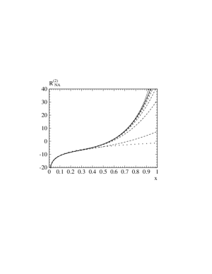
Figure 2: The abelian contribution $R_{A}^{(2)}$, the non-abelian piece $R_{\it NA}^{(2)}$, the contribution from light internal quark loops $R_{l}^{(2)}$ and the contribution $R_{F}^{(2)}$ from the double-bubble diagram with the heavy fermion in both the inner and outer loop as functions of $x=2m/\sqrt{s}$. Wide dots: no mass terms; dashed lines: including mass terms $(m^{2}/s)^{n}$ up to $n=5$; solid line: including mass terms up to $(m^{2}/s)^{6}$; narrow dots: semi-analytical result (except for $R_{F}^{(2)}$). The scale $\mu^{2}=m^{2}$ has been adopted.

Figure 3: $R_{i}^{(2)},i=A,{\it NA},l,F$ for $\mu^{2}=s$ including successively higher orders in $m^{2}/s$. The same notation as in Fig. 2 is adopted. The semi-analytical result is not shown.

Figure 4: $R_{\it NA}^{(2)}-R_{g}^{(2)}(\xi=4)$ over $x=2m/\sqrt{s}$. Dotted: semi-analytical result; dashed: mass terms up to $(m^{2}/s)^{5}$; solid: mass terms up to $(m^{2}/s)^{6}$.

Figure 5: Comparison between the analytical result without 4-particle contribution ($R^{(2)}_{F,virt}$, dotted line) and approximate result with terms up to order $(m^{2}/s)^{5}$ (dashed) and $(m^{2}/s)^{6}$ (solid line).

Let us discuss separately the high energy and the low energy regions. For all three functions $R_{A}$, $R_{\it NA}$ and $R_{l}$ and values between $x=0$ and $x=0.6$ ($x=2m/\sqrt{s}$) the expansions including terms of order $(m^{2}/s)^{3}$ (or more) are in perfect agreement with the semi-analytical result. Conversely this provides a completely independent test of the method of [8] which did rely mainly on low energy information. Including more terms in the expansion, one obtains an improved approximation even in the low energy region. However, the quality of the “convergence” is significantly better for $R_{l}$ and $R_{\it NA}$ than for $R_{A}$. Two reasons may be responsible for this difference: (i) In a high energy expansion it is presumably more difficult to approximate the $1/v$ Coulomb singularity in $R_{A}$ than the mild $\ln v$ singularity in $R_{\it NA}$ and $R_{l}$. (ii) The function $R_{l}$ can be approximated in the whole energy region $2m<\sqrt{s}<\infty$ by an increasing number of terms with arbitrary accuracy. This is evident from the known analytical form of $R_{l}$, a consequence of the absence of thresholds above $2m$ in this piece. In contrast the functions $R_{A}$ and $R_{\it NA}$ exhibit a four particle threshold at $\sqrt{s}=4m$. The high energy expansion is, therefore, not expected to converge to the correct answer in the interval between $2m$ and $4m$. For $R_{\it NA}$ this feature can be studied in more detail by separating $R_{\it NA}$ into the gluonic double-bubble terms in the $\xi=4$ gauge [18] and a remainder. This separation is possible both for the semi-analytical result and the expansion (Fig. 4). The remainder approaches a constant both for $x\to 0$ and $x\to 1$. For $0<x<0.5$ the agreement is perfect. It extends even up to $x\approx 0.9$, a fact which is quite remarkable and surprising.

For $R_{F}$ the expansion is also shown in Fig. 2. Again one observes quick convergence for $x$ between $0$ and $0.5$. No (semi-)analytical result is available for the comparison with $R_{F}$. However, in the region below the four particle threshold an analytical result is available, based on the calculation of the form factor in [6]. The four fermion contribution is expected to be small for energies just above $4m$, corresponding to $x$ just below $x=0.5$. Reasonable agreement between the two approaches is therefore expected in the region around $x=0.5$. This is indeed observed in Fig. 5.

5 Summary

An algorithm has been described which produces the asymptotic expansion of the three-loop vacuum polarization automatically. It generates the relevant subdiagrams and assigns the diagrams automatically to the programs MINCER and MATAD which evaluate the resulting massless propagator and massive tadpole integrals. The output is compared to the quartic terms obtained in [5] and to the semi-analytical results of [8], confirming both these earlier results and the validity of the expansion down to fairly low energy values.

References

• [1] K.G. Chetyrkin, A.L. Kataev and F.V. Tkachov, Phys. Lett. B 85 (1979) 227;
M. Dine and J. Sapirstein, Phys. Rev. Lett. 43 (1979) 668;
W. Celmaster and R.J. Gonsalves, Phys. Rev. Lett. 44 (1980) 560.
• [2] S.G. Gorishny, A.L. Kataev and S.A. Larin, Phys. Lett. B 259 (1991) 144;
L.R. Surguladze and M.A. Samuel, Phys. Rev. Lett. 66 (1991) 560; erratum ibid., 2416;
K.G. Chetyrkin, Phys. Lett. B 391 (1997) 402.
• [3] S.G. Gorishny, A.L. Kataev and S.A. Larin, Nuovo Cim. 92A (1986) 119.
• [4] K.G. Chetyrkin and J.H. Kühn, Phys. Lett. B 248 (1990) 359.
• [5] K.G. Chetyrkin and J.H. Kühn, Nucl. Phys. B 432 (1994) 337.
• [6] A.H. Hoang, J.H. Kühn and T. Teubner, Nucl. Phys. B 452 (1995) 173.
• [7] A.H. Hoang, M. Jeżabek, J.H. Kühn and T. Teubner, Phys. Lett. B 338 (1994) 330.
• [8] K.G. Chetyrkin, J.H. Kühn and M. Steinhauser, Phys. Lett. B 371 (1996) 93; Nucl. Phys. B 482 (1996) 213.
• [9] V.A. Smirnov, Mod. Phys. Lett. A 10 (1995) 1485.
• [10] S.G. Gorishny, preprints JINR E2-86-176, E2-86-177 (Dubna, 1986); Nucl. Phys. B 319 (1989) 633;
K.G. Chetyrkin and V.A. Smirnov, preprint INR G-518 (Mocow, 1987);
K.G. Chetyrkin, Teor. Mat. Fiz 75 (1988) 26; ibid. 76 (1988) 207.
• [11] J.A.M. Vermaseren, Symbolic Manipulation with FORM, (Computer Algebra Netherlands, Amsterdam, 1991).
• [12] S.A. Larin, F.V. Tkachov and J.A.M. Vermaseren, Preprint NIKHEF-H/91-18, (1991).
• [13] D.J. Broadhurst, Z. Phys. C 54 (1992) 54.
• [14] K.G. Chetyrkin, R. Harlander, J.H. Kühn and M. Steinhauser, in Proceedings of the 5th International Workshop on New Computing Techniques in Physics Research: Software Engineering, Neural Nets, Genetic Algorithms, Expert Systems, Symbolic Algebra, Automatic Calculations (AIHENP 96), Lausanne, Switzerland, 2–6 September 1996; Report Nos. MPI/PhT/96-122, TTP96-55 and hep-ph/9611354.
• [15] D.J. Broadhurst and S.C. Generalis, Preprint OUT-4102-12, (1984).
• [16] K.G. Chetyrkin and V.P. Spiridonov, Yad. Fiz. 47 (1988) 818.
• [17] N. Gray, D.J. Broadhurst, W. Grafe, and K. Schilcher, Z. Phys. C 48 (1990) 673.
• [18] K.G. Chetyrkin, A.H. Hoang, J.H. Kühn, M. Steinhauser and T. Teubner, Phys. Lett. B 384 (1996) 233.