$N_{f}=2+1$ QCD thermodynamics with gradient flow using two-loop matching coefficients

Abstract

We study thermodynamic properties of $N_{f}=2+1$ QCD on the lattice adopting a nonperturbatively $O(a)$-improved Wilson quark action and the renormalization group-improved Iwasaki gauge action. To cope with the problems due to explicit violation of the Poincaré and chiral symmetries, we apply the Small Flow-time eXpansion (SFtX) method based on the gradient flow, which is a general method to correctly calculate any renormalized observables on the lattice. In this method, the matching coefficients in front of operators in the small flow-time expansion are calculated by perturbation theory thanks to the asymptotic freedom around the small flow-time limit. In a previous study using one-loop matching coefficients, we found that the SFtX method works well for the equation of state extracted from diagonal components of the energy-momentum tensor and for the chiral condensates and susceptibilities. In this paper, we study the effect of two-loop matching coefficients which have been calculated by Harlander et al.  recently. We also test the influence of the renormalization scale in the SFtX method. We find that, by adopting the $\mu_{0}$ renormalization scale of Harlander et al. instead of the conventional $\mu_{d}=1/\sqrt{8t}$ scale, the linear behavior at large flow-times is improved so that we can perform the $t\to 0$ extrapolation of the SFtX method more confidently. In the calculation of the two-loop matching coefficients by Harlander et al., the equation of motion for quark fields was used. For the entropy density in which the equation of motion has no effects, we find that the results using the two-loop coefficients agree well with those using one-loop coefficients. On the other hand, for the trace anomaly which is affected by the equation of motion, we find discrepancies between the one- and two-loop results at high temperatures. By comparing the results of one-loop coefficients with and without using the equation of motion, the main origin of the discrepancies is suggested to be attributed to contamination of $O\!\left((aT)^{2}\right)=O\!\left(1/N_{t}^{2}\right)$ discretization errors in the equation of motion at $N_{t}\mathrel{\hbox to0.0pt{\raise 2.20013pt\hbox{$<$}\hss}{\lower 2.20013pt\hbox{$\sim$}}}10$.

I Introduction

The gradient flow (GF) opened us a variety of new methods to significantly simplify the calculation of physical observables on the lattice Narayanan:2006rf ; Luscher:2009eq ; Luscher:2010iy ; Luscher:2011bx ; Luscher:2013cpa . For reviews, see Refs. Luscher:2013vga ; Ramos:2015dla ; Lat16suzuki . In this paper, we study finite-temperature QCD with $2+1$ flavors of dynamical quarks by applying the Small Flow-time eXpansion (SFtX) method based on the GF Suzuki:2013gza ; Makino:2014taa ; Endo:2015iea ; Hieda:2016lly .

The GF modifies the fields according to a flow equation, which is given by the gradient of the action in the case of pure Yang-Mills theory and is a kind of diffusion equation in term of a fictitious time (flow-time) $t$. Fields at positive flow-time $t>0$ can be viewed as smeared fields averaged over a mean-square physical radius of $\sqrt{8t}$ in four dimensions. Salient features of the GF are the UV-finiteness and the absence of short-distance singularities in the expectation values of operators constructed by flowed fields at $t>0$. This finiteness enables us to identify these expectation values and corresponding operators as renormalized ones. We call this renormalization scheme as GF-scheme.

At small flow-times, operators in the GF-scheme (“flowed operators”) can be expanded in terms of operators at $t=0$ in a conventional renormalization scheme, say the $\overline{\textrm{MS}}$-scheme Luscher:2011bx . By inverting the relation, we can also expand correctly renormalized physical observables in conventional schemes in terms of flowed operators at small $t$. Thanks to the asymptotic freedom of QCD around the small flow-time limit, we can calculate the matching coefficients relating the operators in two schemes by perturbation theory. Basic idea of the SFtX method is that, because the flowed operators are finite, we can evaluate their expectation values directly on the lattice without further renormalization Suzuki:2013gza . We can thus extract the values of correctly renormalized physical observables by extrapolating proper combinations of expectation values in the GF-scheme to the small flow-time limit $t\to 0$. In these extrapolations, the matching coefficients act not only to match the renormalization schemes but also to make the $t$-dependence milder by removing calculable part of operator mixings and $t$-dependences around the small flow-time limit. Note that the method is applicable also to observables whose founding symmetry is violated explicitly on the lattice, provided that the lattice theory has the correct continuum limit in which the symmetry is restored.

The SFtX method was first tested in quenched QCD to calculate the energy-momentum tensor (EMT) Asakawa:2013laa ; FlowQCD1 ; Iritani2019 ; Yanagihara2018 , which has not been easy to evaluate on the lattice due to the explicit violation of the Poincaré invariance by the lattice regularization. It was found that the equation of state (EoS) calculated from the diagonal components of the EMT correctly reproduces previous estimation using the conventional integral methods Boyd:1996bx ; Okamoto:1999hi ; Umeda:2008bd ; Borsanyi:2012ve . The SFtX method was tested successfully also in solvable models Makino:2014cxa ; Suzuki:2015fka .

We note that the SFtX method is applicable also to chiral observables Endo:2015iea ; Hieda:2016lly . We thus apply the method to QCD with dynamical Wilson-type quarks, with which the correct continuum limit is guaranteed, to cope with the problems due to explicit violation of the chiral symmetry on the lattice Taniguchi:2016ofw ; Taniguchi:2016tjc ; Lat2017-kanaya ; Taniguchi:2017ibr . To reduce the finite lattice spacing effects, we adopt the renormalization-group improved Iwasaki gauge action Iwasaki:2011np ; Iwasaki:1985we and the $O(a)$-improved Wilson quark action Sheikholeslami:1985ij with a nonperturbatively estimated clover coefficient using the Schrödinger functional method SAoki2006 .

In our previous study of $(2+1)$-flavor QCD with slightly heavy $u$ and $d$ quarks ($m_{\pi}/m_{\rho}\simeq 0.63$) and approximately physical $s$ quark ($m_{\eta_{ss}}/m_{\phi}\simeq 0.74$), we calculated the EMT as well as chiral condensates and disconnected chiral susceptibilities in the temperature range of $T\simeq 174$–697 MeV ($N_{t}=16$–4, where $N_{t}$ is the lattice size in the temporal direction) Taniguchi:2016ofw . The lattices are relatively fine with the lattice spacing $a\simeq 0.07$ fm. Adopting one-loop matching coefficients calculated in Refs. Makino:2014taa ; Hieda:2016lly , we found that the EoS extracted from diagonal components of EMT by the SFtX method is well consistent with that estimated with the conventional $T$-integration method at $T\mathrel{\hbox to0.0pt{\raise 2.20013pt\hbox{$<$}\hss}{\lower 2.20013pt\hbox{$\sim$}}}280\,\mathrm{MeV}$ ($N_{t}\mathrel{\hbox to0.0pt{\raise 2.20013pt\hbox{$>$}\hss}{\lower 2.20013pt\hbox{$\sim$}}}10$) Umeda:2012er . At the same time, the two estimates of EoS deviate at $T\mathrel{\hbox to0.0pt{\raise 2.20013pt\hbox{$>$}\hss}{\lower 2.20013pt\hbox{$\sim$}}}348\,\mathrm{MeV}$, suggesting contamination of $a$-independent lattice artifacts of $O\!\left((aT)^{2}=1/N_{t}^{2}\right)$ at $N_{t}\mathrel{\hbox to0.0pt{\raise 2.20013pt\hbox{$<$}\hss}{\lower 2.20013pt\hbox{$\sim$}}}8$ in the EMT. We also found that the chiral condensates bend sharply and the disconnected chiral susceptibilities show peak at $T\simeq 190$ MeV which was suggested as the pseudocritical temperature from other observables Umeda:2012er . We have further studied topological properties of QCD by the SFtX method on these lattices Taniguchi:2016tjc . We found that the topological susceptibilities estimated with the gluonic and fermionic definitions agree well with each other at $T\mathrel{\hbox to0.0pt{\raise 2.20013pt\hbox{$<$}\hss}{\lower 2.20013pt\hbox{$\sim$}}}279$ MeV even at finite lattice spacing of $a=0.07$ fm. This is in clear contrast to their conventional lattice estimations: For example, a study with improved staggered quarks reports more than hundred times larger gluonic susceptibility than fermionic one at similar lattice spacings Petreczky:2016vrs . These suggest that the SFtX method is powerful in calculating observables from lattice simulations.

Recently, Harlander, Kluth, and Lange have completed the calculation of the matching coefficients for EMT up to the two-loop order Harlander:2018zpi . Some details of their calculation are given in AHLNP . Removing more known small-$t$ behaviors, we may perhaps expect milder $t$-dependence in the $t\rightarrow 0$ extrapolation. The two-loop coefficients were first tested in quenched QCD Iritani2019 . It was found that the results of EoS with one- and two-loop coefficients are well consistent with each other. It was also noted that the two-loop coefficients lead to a milder $t$-dependence such that systematic errors from the $t\to 0$ extrapolation are reduced.

In this paper, we extend the test of two-loop coefficients to QCD with $(2+1)$-flavors of dynamical quarks. The lattice setup is the same as in Ref. Taniguchi:2016ofw . A point to be noted here is that, unlike the one-loop coefficients of Ref. Makino:2014taa , in the calculation of two-loop coefficients of Ref. Harlander:2018zpi , the equation of motion (EoM) in the continuum,

$$\bar{\psi}_{f}(x)\left(\frac{1}{2}\stackrel{{\scriptstyle\leftrightarrow}}{{\not\!\!D}}+m_{0,f}\right)\psi_{f}(x)=0,$$ (1)

is used for quark operators, where $\overleftrightarrow{D}_{\mu}\equiv D_{\mu}-\overleftarrow{D}_{\mu}$ and $m_{0,f}$ is the bare quark mass for the $f$’th flavor. With this EoM, we can reduce the number of independent operators and coefficients for EMT. This should cause no effects after taking the continuum limit when the EMT operators are isolated. On finite lattices, however, the EoM gets $O(a)$ lattice corrections which may shift the results for the EMT.

Another point to be addressed in this paper is a technical issue of the choice of the renormalization scale in the matching coefficients of the SFtX method. As shown explicitly in Sec. II, the matching coefficients are written in terms of the flow-time $t$, the running coupling $g$ and masses $m_{f}$ in the $\overline{\textrm{MS}}$ scheme at the renormalization scale $\mu$, and $\mu$ itself. Here, $\mu$ is free to choose as far as the perturbative expansion is valid — the final results for physical observables should be insensitive to the choice of $\mu$. In numerical procedures, however, the perturbative expansion is truncated at a finite order and neglected higher-order corrections in the matching coefficients may cause errors in the results. Because the quality of the perturbative expansion is affected by the choice of $\mu$, we may control these errors to some extent by an appropriate choice of $\mu$. We show that the $\mu_{0}$-scale proposed by Harlander et al. Harlander:2018zpi helps us to have better signals over the conventional choice $\mu_{d}=1/\sqrt{8t}$.

This paper is organized as follows: In Sec. II, we summarize the essence of the SFtX method and introduce the one- and two-loop matching coefficients. Our simulation parameters are given in Sec. III. We then discuss the issue of the renormalization scale in Sec. IV. Our test of two-loop matching coefficients are shown in Sec. V. A summary is given in Sec. VI. In Appendix A, we define the group factors appearing in perturbative expressions of the matching coefficients. In Appendix B, we confirm that the one-loop coefficients of Ref. Makino:2014taa are consistent with the one-loop part of Ref. Harlander:2018zpi .

II The SFtX method

II.1 Gradient flow

Our flow equations are identical to those given in Refs. Luscher:2010iy and Luscher:2013cpa . That is, for the gauge field, we set

$$\partial_{t}B_{\mu}(t,x)=D_{\nu}G_{\nu\mu}(t,x),\qquad B_{\mu}(t=0,x)=A_{\mu}(x),$$ (2)

where the field strength and the covariant derivative of the flowed gauge field are

$$G_{\mu\nu}(t,x)=\partial_{\mu}B_{\nu}(t,x)-\partial_{\nu}B_{\mu}(t,x)+[B_{\mu}(t,x),B_{\nu}(t,x)],$$ (3)

and

$$D_{\nu}G_{\nu\mu}(t,x)=\partial_{\nu}G_{\nu\mu}(t,x)+[B_{\nu}(t,x),G_{\nu\mu}(t,x)],$$ (4)

respectively. For the quark fields, we set

$$\partial_{t}\chi_{f}(t,x)=\Delta\chi_{f}(t,x),\qquad\chi_{f}(t=0,x)=\psi_{f}(x),$$ (5)

$$\partial_{t}\bar{\chi}_{f}(t,x)=\bar{\chi}_{f}(t,x)\overleftarrow{\Delta},\qquad\bar{\chi}_{f}(t=0,x)=\bar{\psi}_{f}(x),$$ (6)

where $f=u$, $d$, $s$, denotes the flavor index, and

$$\Delta\chi_{f}(t,x)\equiv D_{\mu}D_{\mu}\chi_{f}(t,x),\qquad D_{\mu}\chi_{f}(t,x)\equiv\left[\partial_{\mu}+B_{\mu}(t,x)\right]\chi_{f}(t,x),$$ (7)

$$\bar{\chi}_{f}(t,x)\overleftarrow{\Delta}\equiv\bar{\chi}_{f}(t,x)\overleftarrow{D}_{\mu}\overleftarrow{D}_{\mu},\qquad\bar{\chi}_{f}(t,x)\overleftarrow{D}_{\mu}\equiv\bar{\chi}_{f}(t,x)\left[\overleftarrow{\partial}_{\mu}-B_{\mu}(t,x)\right].$$ (8)

Note that our flow equations are independent of the flavor.

II.2 Energy-momentum tensor with two-loop matching coefficients

In terms of unflowed operators, the EMT under the dimensional regularization is given by

$$T_{\mu\nu}(x)=\frac{1}{g_{0}^{2}}\left[\mathcal{O}_{1,\mu\nu}(x)-\frac{1}{4}\mathcal{O}_{2,\mu\nu}(x)\right]+\frac{1}{4}\mathcal{O}_{3,\mu\nu}(x)-\frac{1}{2}\mathcal{O}_{4,\mu\nu}(x)-\mathcal{O}_{5,\mu\nu}(x),$$ (9)

where

$$\mathcal{O}_{1,\mu\nu}(x) \equiv F_{\mu\rho}^{a}(x)F_{\nu\rho}^{a}(x),$$ (10)

$$\mathcal{O}_{2,\mu\nu}(x) \equiv\delta_{\mu\nu}F_{\rho\sigma}^{a}(x)F_{\rho\sigma}^{a}(x),$$ (11)

$$\mathcal{O}_{3,\mu\nu}(x) \equiv\sum_{f}\bar{\psi}_{f}(x)\left(\gamma_{\mu}\overleftrightarrow{D}_{\nu}+\gamma_{\nu}\overleftrightarrow{D}_{\mu}\right)\psi_{f}(x),$$ (12)

$$\mathcal{O}_{4,\mu\nu}(x) \equiv\delta_{\mu\nu}\sum_{f}\bar{\psi}_{f}(x)\overleftrightarrow{{\ooalign{\hfil/\hfil\crcr$D$}}}\psi_{f}(x),$$ (15)

$$\mathcal{O}_{5,\mu\nu}(x) \equiv\delta_{\mu\nu}\sum_{f}m_{f,0}\bar{\psi}_{f}(x)\psi_{f}(x),$$ (16)

with $F_{\mu\nu}^{a}(x)$ the field strength of unflowed gauge field $A^{a}_{\mu}(x)$. Here and in what follows, we assume for notational simplicity that the vacuum expectation value (VEV), i.e., the expectation value at zero-temperature, is subtracted in each operator.

In terms of flowed operators,

$$\tilde{\mathcal{O}}_{1,\mu\nu}(t,x) \equiv G_{\mu\rho}^{a}(t,x)G_{\nu\rho}^{a}(t,x),$$ (17)

$$\tilde{\mathcal{O}}_{2,\mu\nu}(t,x) \equiv\delta_{\mu\nu}G_{\rho\sigma}^{a}(t,x)G_{\rho\sigma}^{a}(t,x),$$ (18)

$$\tilde{\mathcal{O}}_{3,\mu\nu}(t,x) \equiv\sum_{f}\mathring{\bar{\chi}}_{f}(t,x)\left(\gamma_{\mu}\overleftrightarrow{D}_{\nu}+\gamma_{\nu}\overleftrightarrow{D}_{\mu}\right)\mathring{\chi}_{f}(t,x),$$ (19)

$$\tilde{\mathcal{O}}_{4,\mu\nu}(t,x) \equiv\delta_{\mu\nu}\sum_{f}\mathring{\bar{\chi}}_{f}(t,x)\overleftrightarrow{{\ooalign{\hfil/\hfil\crcr$D$}}}\mathring{\chi}_{f}(t,x),$$ (22)

$$\tilde{\mathcal{O}}_{5,\mu\nu}(t,x) \equiv\delta_{\mu\nu}\sum_{f}m_{f}\mathring{\bar{\chi}}_{f}(t,x)\mathring{\chi}_{f}(t,x),$$ (23)

the EMT is expressed as Makino:2014taa ; Taniguchi:2016ofw

$$T_{\mu\nu}(x)= \,c_{1}(t)\left[\tilde{\mathcal{O}}_{1,\mu\nu}(t,x)-\frac{1}{4}\tilde{\mathcal{O}}_{2,\mu\nu}(t,x)\right]+c_{2}(t)\tilde{\mathcal{O}}_{2,\mu\nu}(t,x)$$

$$+c_{3}(t)\left[\tilde{\mathcal{O}}_{3,\mu\nu}(t,x)-2\tilde{\mathcal{O}}_{4,\mu\nu}(t,x)\right]+c_{4}(t)\tilde{\mathcal{O}}_{4,\mu\nu}(t,x)$$

$$+c_{5}(t)\tilde{\mathcal{O}}_{5,\mu\nu}(t,x)+O(t),$$ (24)

where

$$\mathring{\chi}_{f}(t,x) \equiv\sqrt{\frac{-2\dim(R)}{(4\pi)^{2}t^{2}\left\langle\bar{\chi}_{f}(t,x)\overleftrightarrow{{\ooalign{\hfil/\hfil\crcr$D$}}}\chi_{f}(t,x)\right\rangle}}\,\chi_{f}(t,x),$$ (27)

$$\mathring{\bar{\chi}}_{f}(t,x) \equiv\sqrt{\frac{-2\dim(R)}{(4\pi)^{2}t^{2}\left\langle\bar{\chi}_{f}(t,x)\overleftrightarrow{{\ooalign{\hfil/\hfil\crcr$D$}}}\chi_{f}(t,x)\right\rangle}}\,\bar{\chi}_{f}(t,x),$$ (30)

are “ringed” quark fields introduced in Ref. Makino:2014taa to carry out a wave function renormalization of quark fields nonperturbatively, where the operators in the denominator are not VEV-subtracted. The $O(t)$ term in the right-hand side of Eq. (24) can be removed by a $t\to 0$ extrapolation. Explicit forms of the matching coefficients $c_{1}$, $\cdots$, $c_{5}$ to the one-loop order (NLO) are given in Ref. Makino:2014taa .

Recently, two-loop (NNLO) calculation of the matching coefficients has been completed by Harlander, Kluth, and Lange Harlander:2018zpi . Unlike the calculation of Ref. Makino:2014taa , the EoM (1) was used in Ref. Harlander:2018zpi assuming that the EMT operators are spatially separated from other composite operators. See also Sec. 5 of Ref. Makino:2014taa . In terms of unflowed operators, Eq. (1) reads as

$$\frac{1}{2}\mathcal{O}_{4,\mu\nu}(x)+\mathcal{O}_{5,\mu\nu}(x)=0.$$ (31)

Note that Eq. (31) implies that the last two terms of Eq. (9) cancel with each other:

$$T_{\mu\nu}(x)=\frac{1}{g_{0}^{2}}\left[\mathcal{O}_{1,\mu\nu}(x)-\frac{1}{4}\mathcal{O}_{2,\mu\nu}(x)\right]+\frac{1}{4}\mathcal{O}_{3,\mu\nu}(x).$$ (32)

In terms of the flowed operators, the EoM is

$$\delta_{\mu\nu}\sum_{f}\left[\bar{\psi}_{f}(x)\left(\overleftrightarrow{{\ooalign{\hfil/\hfil\crcr$D$}}}+2m_{f,0}\right)\psi_{f}(x)\right]$$ (35)

$$=d_{2}(t)\tilde{\mathcal{O}}_{2,\mu\nu}(t,x)+\mathring{d}_{4}(t)\tilde{\mathcal{O}}_{4,\mu\nu}(t,x)+\mathring{d}_{5}(t)\tilde{\mathcal{O}}_{5,\mu\nu}(t,x)+O(t)=0,$$ (36)

where, in the one-loop level, the coefficients $d_{i}(t)$ are given by (cf. Eqs. (5.3)–(5.5) of Ref. Makino:2014taa )

$$d_{2}(t) =\frac{1}{4g^{2}}\frac{g^{2}}{(4\pi)^{2}}\left(-\frac{20}{3}\right)T_{F},$$ (37)

$$\mathring{d}_{4}(t) =1+\frac{g^{2}}{(4\pi)^{2}}C_{F}\left(-\frac{1}{2}+\ln 432\right),$$ (38)

$$\mathring{d}_{5}(t) =2\left\{1+\frac{g^{2}}{(4\pi)^{2}}C_{F}\left[3L(\mu,t)+2+\ln 432\right]\right\}.$$ (39)

where $g$ is the running coupling in the $\overline{\textrm{MS}}$-scheme at the renormalization scale $\mu$, and

$$L(\mu,t)\equiv\ln(2\mu^{2}t)+\gamma_{E}$$ (40)

with $\gamma_{E}$ the Euler-Mascheroni constant. The definitions of the group factors ($T_{F}$ etc.) are summarized in Appendix A.

Using Eq. (36), we can eliminate $\tilde{\mathcal{O}}_{5,\mu\nu}(t,x)$ order by order in perturbation theory (up to $O(t)$ terms), to obtain

$$T_{\mu\nu}(x)=\check{c}_{1}(t)\tilde{\mathcal{O}}_{1,\mu\nu}(t,x)+\check{c}_{2}(t)\tilde{\mathcal{O}}_{2,\mu\nu}(t,x)+\mathring{\check{c}}_{3}(t)\tilde{\mathcal{O}}_{3,\mu\nu}(t,x)+\mathring{\check{c}}_{4}(t)\tilde{\mathcal{O}}_{4,\mu\nu}(t,x)+O(t).$$ (41)

The matching coefficients $\check{c}_{1}(t)$ and $\check{c}_{2}(t)$ to the two-loop order are given in Ref. Harlander:2018zpi as

$$\check{c}_{1}(t)$$

$$=\frac{1}{g^{2}}\biggl{(}1+\frac{g^{2}}{(4\pi)^{2}}\left[-\beta_{0}L(\mu,t)-\frac{7}{3}C_{\!A}+\frac{3}{2}T_{F}\right]$$

$$\quad{}+\frac{g^{4}}{(4\pi)^{4}}\biggl{\{}-\beta_{1}L(\mu,t)+{C_{\!A}}^{2}\left(-\frac{14482}{405}-\frac{16546}{135}\ln 2+\frac{1187}{10}\ln 3\right)$$

$$\qquad\qquad\quad{}+C_{\!A}T_{F}\left[\frac{59}{9}\operatorname{Li}_{2}\left(\frac{1}{4}\right)+\frac{10873}{810}+\frac{73}{54}\pi^{2}-\frac{2773}{135}\ln 2+\frac{302}{45}\ln 3\right]$$

$$\qquad\qquad\quad{}+C_{F}T_{F}\left[-\frac{256}{9}\operatorname{Li}_{2}\left(\frac{1}{4}\right)+\frac{2587}{108}-\frac{7}{9}\pi^{2}-\frac{106}{9}\ln 2-\frac{161}{18}\ln 3\right]\biggr{\}}\biggr{)},$$ (42)

$$\check{c}_{2}(t)$$

$$=\frac{1}{4g^{2}}\biggl{(}-1+\frac{g^{2}}{(4\pi)^{2}}\left[\beta_{0}L(\mu,t)+\frac{25}{6}C_{\!A}-3T_{F}\right]$$

$$\quad{}+\frac{g^{4}}{(4\pi)^{4}}\biggl{\{}\beta_{1}L(\mu,t)+{C_{\!A}}^{2}\left(\frac{56713}{1620}-\frac{1187}{10}\ln 3+\frac{16546}{135}\ln 2\right)$$

$$\qquad\qquad\quad{}+C_{\!A}T_{F}\left[-\frac{59}{9}\operatorname{Li}_{2}\left(\frac{1}{4}\right)-\frac{6071}{405}-\frac{73}{54}\pi^{2}+\frac{2287}{135}\ln 2-\frac{361}{90}\ln 3\right]$$

$$\qquad\qquad\quad{}+C_{F}T_{F}\left[\frac{220}{9}\operatorname{Li}_{2}\left(\frac{1}{4}\right)-\frac{1757}{54}+\frac{10}{9}\pi^{2}-\frac{164}{9}\ln 2+\frac{247}{9}\ln 3\right]\biggr{\}}\biggl{)},$$ (43)

where $\operatorname{Li}_{2}(z)$ is the dilogarithm function with $\operatorname{Li}_{2}(1/4)=0.26765263908\cdots$, and $\beta_{0}$ and $\beta_{1}$ are the first two coefficients of the beta function,

$$\beta_{0} =\frac{11}{3}C_{\!A}-\frac{4}{3}T_{F},$$ (44)

$$\beta_{1} =\frac{34}{3}{C_{\!A}}^{2}-\left(4C_{F}+\frac{20}{3}C_{\!A}\right)T_{F}.$$ (45)

The matching coefficients $\mathring{\check{c}}_{3}(t)$ and $\mathring{\check{c}}_{4}(t)$ are given by

$$\mathring{\check{c}}_{i}(t)\equiv\check{c}_{i}(t)\zeta_{\chi}(t)^{-1},\qquad\text{for $i=3$, $4$},$$ (46)

using

$$\check{c}_{3}(t)$$

$$=\frac{1}{4}\biggl{(}1+\frac{g^{2}}{(4\pi)^{2}}\left[\frac{3}{2}C_{F}+\frac{\gamma_{\chi,0}}{2}L(\mu,t)\right]$$

$$\quad{}+\frac{g^{4}}{(4\pi)^{4}}\biggl{\{}\frac{\gamma_{\chi,0}}{4}\left(\beta_{0}+\frac{\gamma_{\chi,0}}{2}\right)\left[L(\mu,t)^{2}+L(\mu,t)\right]+\frac{\gamma_{\chi,1}}{2}L(\mu,t)$$

$$\qquad\qquad\quad{}+C_{F}^{2}\left[-\frac{137}{9}\operatorname{Li}_{2}\left(\frac{1}{4}\right)-\frac{559}{216}+\frac{103}{108}\pi^{2}-\frac{1736}{27}\ln 2+\frac{122}{3}\ln 3-4(\ln 2)^{2}\right]$$

$$\qquad\qquad\quad{}+C_{F}T_{F}\left[-\frac{136}{9}\operatorname{Li}_{2}\left(\frac{1}{4}\right)-\frac{3377}{810}-\frac{7}{9}\pi^{2}+\frac{1232}{135}\ln 2-\frac{136}{15}\ln 3\right]$$

$$\qquad\qquad\quad{}+C_{\!A}C_{F}\left[-\frac{365}{9}\operatorname{Li}_{2}\left(\frac{1}{4}\right)+\frac{261829}{3240}+\frac{77}{108}\pi^{2}+\frac{5788}{45}\ln 2-\frac{2102}{15}\ln 3-4(\ln 2)^{2}\right]\biggr{\}}\biggr{)},$$ (47)

and

$$\check{c}_{4}(t)$$

$$=\frac{C_{F}}{2}\biggl{(}\frac{g^{2}}{(4\pi)^{2}}$$

$$\quad{}+\frac{g^{4}}{(4\pi)^{4}}\biggl{\{}\left[\beta_{0}+\frac{\gamma_{\chi,0}}{2}\right]L(\mu,t)$$

$$\qquad\qquad\quad{}+C_{F}\left[-\frac{161}{18}\operatorname{Li}_{2}\left(\frac{1}{4}\right)-\frac{41}{54}-\frac{55}{108}\pi^{2}-\frac{1105}{27}\ln 2+\frac{101}{6}\ln 3\right]$$

$$\qquad\qquad\quad{}+T_{F}\left[\frac{25}{9}\operatorname{Li}_{2}\left(\frac{1}{4}\right)-\frac{20573}{1620}+\frac{5}{18}\pi^{2}+\frac{6559}{135}\ln 2-\frac{679}{30}\ln 3\right]$$

$$\qquad\qquad\quad{}+C_{\!A}\left[\frac{257}{36}\operatorname{Li}_{2}\left(\frac{1}{4}\right)-\frac{137}{405}+\frac{11}{216}\pi^{2}-\frac{419}{90}\ln 2+\frac{1157}{60}\ln 3\right]\biggr{\}}\biggr{)},$$ (48)

given in Ref. Harlander:2018zpi , where

$$\gamma_{\chi,0} =6C_{F},$$ (49)

$$\gamma_{\chi,1} =C_{\!A}C_{F}\left(\frac{223}{3}-16\ln 2\right)-C_{F}^{2}(3+16\ln 2)-\frac{44}{3}C_{F}T_{F}.$$ (50)

Here, $\zeta_{\chi}(t)$ adjusts the normalization of quark fields to that of the ringed variables in Eqs. (27) and (30), and is given by

$$\zeta_{\chi}(t)$$

$$=1+\frac{g^{2}}{(4\pi)^{2}}\left[\frac{\gamma_{\chi,0}}{2}L(\mu,t)-3C_{F}\ln 3-4C_{F}\ln 2\right]$$

$$\qquad{}+\frac{g^{4}}{(4\pi)^{4}}\Bigl{\{}\frac{\gamma_{\chi,0}}{4}\left(\beta_{0}+\frac{\gamma_{\chi,0}}{2}\right)L(\mu,t)^{2}$$

$$\qquad\qquad\qquad{}+\left[\frac{\gamma_{\chi,1}}{2}-\frac{\gamma_{\chi,0}}{2}\left(\beta_{0}+\frac{\gamma_{\chi,0}}{2}\right)\ln 3-\frac{2}{3}\gamma_{\chi,0}\left(\beta_{0}+\frac{\gamma_{\chi,0}}{2}\right)\ln 2\right]L(\mu,t)$$

$$\qquad\qquad\qquad{}+C_{2}\Bigr{\}},$$ (51)

with

$$C_{2}\equiv-23.8C_{\!A}C_{F}+30.4C_{F}^{2}-3.92C_{F}T_{F}.$$ (52)

Its inverse reads as

$$\zeta_{\chi}(t)^{-1}$$

$$=1+\frac{g^{2}}{(4\pi)^{2}}\left[-\frac{\gamma_{\chi,0}}{2}L(\mu,t)+C_{F}\ln 432\right]$$

$$\qquad{}+\frac{g^{4}}{(4\pi)^{4}}\Bigl{\{}\frac{\gamma_{\chi,0}}{4}\left(-\beta_{0}+\frac{\gamma_{\chi,0}}{2}\right)L(\mu,t)^{2}$$

$$\qquad\qquad\qquad{}+\left[-\frac{\gamma_{\chi,1}}{2}+\frac{\gamma_{\chi,0}}{6}\left(\beta_{0}+\frac{\gamma_{\chi,0}}{2}-6C_{F}\right)\ln 432\right]L(\mu,t)$$

$$\qquad\qquad\qquad{}-C_{2}+C_{F}^{2}(\ln 432)^{2}\Bigr{\}}.$$ (53)

We then obtain

$$\mathring{\check{c}}_{3}(t)$$

$$=\frac{1}{4}\biggl{(}1+\frac{g^{2}}{(4\pi)^{2}}C_{F}\left(\frac{3}{2}+\ln 432\right)$$

$$\quad{}+\frac{g^{4}}{(4\pi)^{4}}\biggl{\{}\frac{\gamma_{\chi,0}}{6}\left(\beta_{0}+\frac{\gamma_{\chi,0}}{2}-3C_{F}\right)\left(\frac{3}{2}+\ln 432\right)L(\mu,t)$$

$$\qquad\qquad\quad{}+C_{F}^{2}\left(\frac{3}{2}+\ln 432\right)\ln 432-C_{2}$$

$$\qquad\qquad\quad{}+C_{F}^{2}\left[-\frac{137}{9}\operatorname{Li}_{2}\left(\frac{1}{4}\right)-\frac{559}{216}+\frac{103}{108}\pi^{2}-\frac{1736}{27}\ln 2+\frac{122}{3}\ln 3-4(\ln 2)^{2}\right]$$

$$\qquad\qquad\quad{}+C_{F}T_{F}\left[-\frac{136}{9}\operatorname{Li}_{2}\left(\frac{1}{4}\right)-\frac{3377}{810}-\frac{7}{9}\pi^{2}+\frac{1232}{135}\ln 2-\frac{136}{15}\ln 3\right]$$

$$\qquad\qquad\quad{}+C_{\!A}C_{F}\left[-\frac{365}{9}\operatorname{Li}_{2}\left(\frac{1}{4}\right)+\frac{261829}{3240}+\frac{77}{108}\pi^{2}+\frac{5788}{45}\ln 2-\frac{2102}{15}\ln 3-4(\ln 2)^{2}\right]\biggr{\}}\biggr{)},$$ (54)

where

$$\mathring{\check{c}}_{4}(t)$$

$$=\frac{C_{F}}{2}\biggl{(}\frac{g^{2}}{(4\pi)^{2}}$$

$$\quad{}+\frac{g^{4}}{(4\pi)^{4}}\biggl{\{}\beta_{0}L(\mu,t)$$

$$\qquad\qquad\quad{}+C_{F}\ln 432$$

$$\qquad\qquad\quad{}+C_{F}\left[-\frac{161}{18}\operatorname{Li}_{2}\left(\frac{1}{4}\right)-\frac{41}{54}-\frac{55}{108}\pi^{2}-\frac{1105}{27}\ln 2+\frac{101}{6}\ln 3\right]$$

$$\qquad\qquad\quad{}+T_{F}\left[\frac{25}{9}\operatorname{Li}_{2}\left(\frac{1}{4}\right)-\frac{20573}{1620}+\frac{5}{18}\pi^{2}+\frac{6559}{135}\ln 2-\frac{679}{30}\ln 3\right]$$

$$\qquad\qquad\quad{}+C_{\!A}\left[\frac{257}{36}\operatorname{Li}_{2}\left(\frac{1}{4}\right)-\frac{137}{405}+\frac{11}{216}\pi^{2}-\frac{419}{90}\ln 2+\frac{1157}{60}\ln 3\right]\biggr{\}}\biggr{)}.$$ (55)

In Appendix B, we confirm that the results of Ref. Makino:2014taa are consistent with the one-loop parts of Eqs. (42)–(55).

From the diagonal components of the EMT, we compute the pressure and the energy density as

$$p/T^{4}=\sum_{i=1}^{3}\langle T_{ii}\rangle/(3T^{4}),\hskip 14.22636pt\epsilon/T^{4}=-\langle T_{00}\rangle/T^{4}.$$ (56)

The entropy density and trace anomaly are then computed as $(\epsilon+p)/T$ and $\epsilon-3p$, respectively.

II.3 Extrapolation to $t\to 0$

To extract physical results of EMT in Eqs. (24), (41), etc., we remove contamination of $O(t)$ terms in the right-hand side of these equations by extrapolating them to $t\to 0$. On finite lattices, lattice artifacts contaminate additionally. With $O(a)$-improved Wilson quarks we adopt, the lattice artifacts start with $O(a^{2})$ and we expect the EMT, for example, to be

$$T_{\mu\nu}(t,x,a) = T_{\mu\nu}(x)+tS_{\mu\nu}(x)+A_{\mu\nu}\frac{a^{2}}{t}+\sum_{f}B^{f}_{\mu\nu}(am_{f})^{2}+C_{\mu\nu}(aT)^{2}$$ (57)

$$+D_{\mu\nu}(a\Lambda_{\mathrm{QCD}})^{2}+a^{2}S^{\prime}_{\mu\nu}(x)+O(a^{4},t^{2}),$$

where $T_{\mu\nu}(x)$ is the physical EMT, $S_{\mu\nu}$ and $S^{\prime}_{\mu\nu}$ are contaminations of dimension-six operators with the same quantum number, and $A_{\mu\nu}$, $B^{f}_{\mu\nu}$, $C_{\mu\nu}$, and $D_{\mu\nu}$ are those from dimension-four operators. Though both $a\to 0$ and $t\to 0$ extrapolations are needed to extract the physical EMT, it is often attractive to reserve the $a\to 0$ extrapolation for a late stage of numerical analyses. To perform a $t\to 0$ extrapolation on finite lattices $a\neq 0$, the influence of singular terms such as $a^{2}/t$ must be suppressed. This will be possible when we have a window in $t$ in which the linear terms dominate (“linear window”) Taniguchi:2016ofw .

We found in the study of Ref. Taniguchi:2016ofw that, depending on the observable and simulation parameters, we do have ranges of $t$ in which the data show well linear behavior. We performed linear $t\to 0$ extrapolation of observables when a linear window is available and obtained reasonable results, as introduced in Sec. I. We think that the success of the SFtX method in Ref. Taniguchi:2016ofw is largely due to the fineness of the lattices studied. In this paper, we adopt the same strategy. We also discuss a method which may be used to improve linear behaviors in Sec. IV.

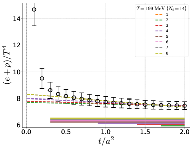
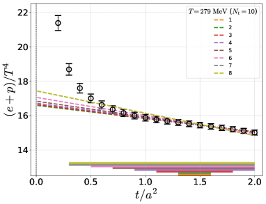
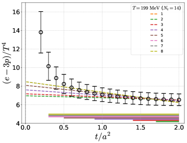
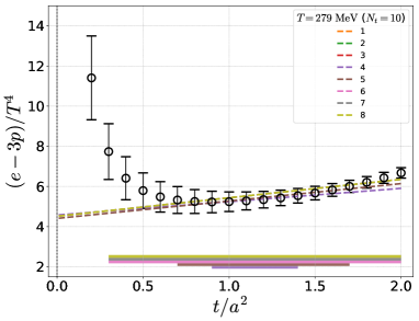
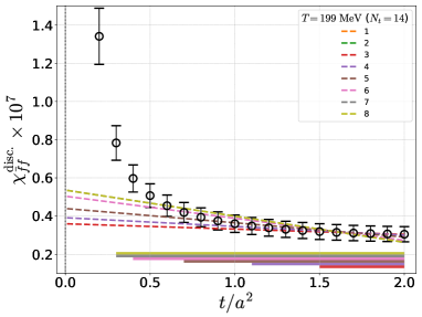
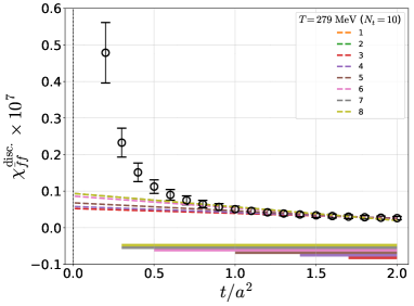
Figure 1: Typical results of the linear fits with the fitting ranges shown by the bands at the bottom of each plot. These fitting ranges are selected by the procedure discussed in Sec. II.3. The cutoff values of $\chi^{2}/N_{\textrm{dof}}$ for the linear fits 1, 2, 3, $\cdots$, and 8 are $10^{-5}$, $10^{-4}$, $10^{-3}$, $\cdots$, and $10^{+2}$, respectively. Results of corresponding linear fits are shown by dashed lines with the same color. The dashed lines with the same fitting range are overlapped with each other, and only the color with the largest fit number is visible. One-loop matching coefficients of Ref. Makino:2014taa and the $\mu_{0}$-scale are adopted. Errors are statistical only.

We identify linear windows as follows: First of all, we require the flow-time to satisfy $\sqrt{2}a\leq\sqrt{8t}\leq\min(N_{t}a/2,N_{s}a/2),$ i.e., the smearing range $\sqrt{8t}$ by the gradient flow covers the minimal lattice separations to make the smearing effective, and, simultaneously, is smaller than the half of the smallest lattice extent to avoid finite-size effects due to overlapped smearing. In terms of the dimensionless flow-time $t/a^{2}$, these conditions read

$$\frac{1}{4}\;\leq\;\frac{t}{a^{2}}\;\leq\;t_{1/2}\equiv\frac{1}{8}\left[\min\left(\frac{N_{t}}{2},\frac{N_{s}}{2}\right)\right]^{2}.$$ (58)

For each observable $\mathcal{O}$, we then look for a range of $t$ in which terms linear in $t$ look dominating, and try linear extrapolations of the form

$$\langle\mathcal{O}(t,a)\rangle=\langle\mathcal{O}\rangle+t\,S_{\mathcal{O}}$$ (59)

with various choices of the fitting range. We then select a temporally best linear fit whose fitting range is the widest within the range (58), under the condition that $\chi^{2}/N_{\textrm{dof}}$ is smaller than a cutoff value. In this study, due to limitation of the statistics, we could not obtain a statistically reliable correlation matrix among data at different flow-times $t$. We thus disregard the correlation among different $t$’s in the calculation of $\chi^{2}/N_{\textrm{dof}}$. This means that the absolute value of $\chi^{2}/N_{\textrm{dof}}$ does not have a strong sense — we can reduce it below any desired value by adding correlated data at intermediate $t$’s. To obtain reasonable fits, we thus repeat the test varying the cutoff value widely. In Fig. 1, we show some typical results of this test. One-loop matching coefficients of Ref. Makino:2014taa and the $\mu_{0}$-scale discussed in Sec. IV are adopted. The cutoffs for the linear fits 1, 2, 3, $\cdots$, and 8 are $10^{-5}$, $10^{-4}$, $10^{-3}$, $\cdots$, and $10^{+2}$, respectively. The selected fitting range for each fit is shown by a line at the bottom of each plot with the same color. From Fig. 1, we note that the linear fits are stable when the cutoff value is large. On the other hand, when we require $\chi^{2}/N_{\textrm{dof}}<10^{-3}$ or smaller, our selection procedure for the temporal linear window becomes sometimes unstable and fails to give a window. Consulting these plots and also requiring that the resulting linear windows are common among similar observables, we decide to choose the fits 5 which require $\chi^{2}/N_{\textrm{dof}}<0.1$ to select optimum linear windows, for all observables we study in this paper.

To confirm the validity of the linear window and to estimate a systematic error due to the fit ansatz, we also make additional fits using the data within the same window: One is a “nonlinear fit” inspired from Eq. (57),

$$\langle\mathcal{O}(t,a)\rangle=\langle\mathcal{O}\rangle+A_{\mathcal{O}}\frac{a^{2}}{t}+t\,S_{\mathcal{O}}+t^{2}R_{\mathcal{O}}.$$ (60)

Another is a “linear+log fit” to estimate the effects of neglected higher-order loop corrections in the matching coefficients. For the case of one-loop matching coefficients, possible corrections are $O(g^{4})\sim O(1/\log^{2}\mu)$. Because $\mu\sim 1/\sqrt{t}$ (see Sec. IV), the leading $t$-dependence of $O(g^{4})$ terms may be taken by fits of the form

$$\langle\mathcal{O}(t,a)\rangle=\langle\mathcal{O}\rangle+t\,S_{\mathcal{O}}+\frac{Q_{\mathcal{O}}}{\log^{2}(\sqrt{8t}\Lambda_{\overline{\mathrm{MS}}})},$$ (61)

where $\Lambda_{\overline{\mathrm{MS}}}=332(17)$ MeV is the QCD lambda parameter for three-flavor QCD quoted in the Particle Data Group PDG . For the case of two-loop matching coefficients, we instead try

$$\langle\mathcal{O}(t,a)\rangle=\langle\mathcal{O}\rangle+t\,S_{\mathcal{O}}+\frac{Q^{\prime}_{\mathcal{O}}}{\log^{3}(\sqrt{8t}\Lambda_{\overline{\mathrm{MS}}})}$$ (62)

to estimate the $O(g^{6})$ contaminations. We take the difference between the linear fit and the nonlinear or linear+log fits as an estimate of the systematic error due to the choice of the fit ansatz.

III Simulation parameters and our numerical methods

The numerical setup for this study is the same as that of Ref. Taniguchi:2016ofw . We study $2+1$ flavor QCD with slightly heavy $u$ and $d$ quarks ($m_{\pi}/m_{\rho}\simeq 0.63$) and approximately physical $s$ quark ($m_{\eta_{ss}}/m_{\phi}\simeq 0.74$) on a relatively fine lattice with the lattice spacing $a\simeq 0.07$ fm ($a^{-1}\simeq 2.79$ GeV) Umeda:2012er ; Ishikawa:2007nn . To reduce the finite lattice spacing effects, we adopt the renormalization-group improved Iwasaki gauge action Iwasaki:2011np ; Iwasaki:1985we and the $O(a)$-improved Wilson quark action Sheikholeslami:1985ij . For the clover coefficients of the improved Wilson quark action, we adopt nonperturbatively evaluated values SAoki2006 . The bare gauge coupling parameter and the hopping parameters are set to $\beta=2.05$, $\kappa_{ud}=0.1356$, and $\kappa_{s}=0.1351$.

Finite temperature configurations in the range of $T\simeq 174$–348 MeV ($N_{t}=16$–8) have been generated adopting the fixed-scale approach Umeda:2012er ; Umeda:2008bd . The values of temperature at each $N_{t}$ are given in Table 1. The spatial box size is $32^{3}$ for $T>0$ and $28^{3}$ for $T=0$. Although we have configurations also at $T\simeq 464$ MeV ($N_{t}=6$) and $T\simeq 697$ MeV ($N_{t}=4$) Taniguchi:2016ofw , limitations by $t_{1/2}=1.125$ and 0.5, respectively, are too severe to obtain a stable linear window. It was also noted that the EoS on $N_{t}\mathrel{\hbox to0.0pt{\raise 2.20013pt\hbox{$<$}\hss}{\lower 2.20013pt\hbox{$\sim$}}}8$ lattices has large $O\!\left((aT)^{2}=1/N_{t}^{2}\right)$ lattice artifacts Taniguchi:2016ofw . We thus just omit these configurations in this study.

Table 1: Simulation parameters: Temperature in MeV, $T/T_{\mathrm{pc}}$ assuming $T_{\mathrm{pc}}=190$ MeV, the temporal lattice size $N_{t}$, $t_{1/2}$ defined by Eq. (58), and the number of configurations used in gauge and fermion measurements. Spatial box size is $32^{3}$ for $T>0$ and $28^{3}$ for $T=0$.

$T$[MeV]	$T/T_{\mathrm{pc}}$	$N_{t}$	$t_{1/2}$	gauge configurations	fermion configurations
$0$	$0$	$56$	$24.5$	$650$	$65$
$174$	$0.92$	$16$	$8$	$1440$	$144$
$199$	$1.05$	$14$	$6.125$	$1270$	$127$
$232$	$1.22$	$12$	$4.5$	$1290$	$129$
$279$	$1.47$	$10$	$3.125$	$780$	$78$
$348$	$1.83$	$8$	$2$	$510$	$51$

Our numerical algorithm for gradient flow is given in Ref. Taniguchi:2016ofw . We adopt the third order Runge-Kutta method with the step size of $\epsilon=0.02$. For the quadratic terms of the field strength tensor $G_{\mu\nu}(x)$, we adopt clover operator with four plaquette Wilson loops and that with eight $1\times 2$ rectangle Wilson loops such that the tree-level improved field strength squared is obtained AliKhan:2001ym . To calculate the $\overline{\textrm{MS}}$ running coupling and masses in the matching coefficients, we adopt five-loop beta and gamma functions FiveLoop , instead of the four-loop functions adopted in our previous study Taniguchi:2016ofw .

We evaluate fermionic observables by the noisy estimator method. The number of noise vectors we adopt is 20 for each color and spinor component. To measure fermionic bilinear observables at $t>0$, instead of the adjoint Runge-Kutta integration adopted in Ref. Taniguchi:2016ofw (see Appendix B of Ref. Taniguchi:2016ofw ), we apply an alternative method using usual forward Runge-Kutta integrations only by locating the noise vectors at $t=0$. See Appendix C for details. We confirm that the both methods give consistent results within statistical errors of the noise method. This alternative method is applicable to fermionic bilinear observables and reduces the computational cost. On the other hand, because the data at all $t$’s are estimated with the same noise vector at $t=0$, the correlation among different $t$’s is stronger than the study of Ref. Taniguchi:2016ofw in which independent noise vectors were generated at each $t$. The gauge observables are measured every 5 trajectories at $T>0$ and every 10 trajectories at $T=0$, while the fermionic observables are measured every 50 trajectories at $T>0$ and every 100 trajectories at $T=0$. The statistical errors are estimated by the standard jackknife analysis with the bin size of 100 trajectories for the energy-momentum tensor and 300 trajectories for the chiral condensates and susceptibilities.

IV Renormalization scale

Our matching coefficients, Eqs. (42)–(55), are functions of the renormalization scale $\mu$ and the  $\overline{\textrm{MS}}$ running coupling constant $g$ at the renormalization scale $\mu$. Here, the renormalization scale $\mu$ is free to choose as long as the perturbative expansion of the matching coefficients is valid because the final physical observables are independent of $\mu$.

A conventional choice of $\mu$ is

$$\mu=\mu_{d}(t)\equiv\frac{1}{\sqrt{8t}},$$ (63)

which is a natural scale of flowed operators because $\sqrt{8t}$ is the physical smearing extent of flowed fields. On the other hand, the authors of Ref. Harlander:2018zpi argued that the choice

$$\mu=\mu_{0}(t)\equiv\frac{e^{-\gamma_{E}/2}}{\sqrt{2t}},$$ (64)

which sets $L(\mu,t)=0$ in Eqs. (42)–(55), keeps the relative contribution of two-loop terms small in a similar level as the $\mu_{d}$-scale.

We note that, since

$$\mu_{0}(t)\simeq 1.4986\times\mu_{d}(t),$$ (65)

the $\mu_{0}$-scale is more perturbative than the $\mu_{d}$-scale in asymptotically free theories. Thus, the $\mu_{0}$-scale may improve the quality of perturbative expressions, in particular at large $t$.

IV.1 Test of renormalization scales using one-loop matching coefficients

In Fig. 2, we examine effects of the renormalization scale by comparing the results for the entropy density,

$$\frac{\epsilon+p}{T^{4}}=-\frac{4}{3T^{4}}\left\langle T_{00}-\frac{1}{4}T_{\mu\mu}\right\rangle,$$ (66)

at finite $t$ with $\mu_{0}$- and $\mu_{d}$-scales. Corresponding results for the trace anomaly,

$$\frac{\epsilon-3p}{T^{4}}=-\frac{1}{T^{4}}\langle T_{\mu\mu}\rangle,$$ (67)

are shown in Fig. 3. We adopt one-loop matching coefficients of Ref. Makino:2014taa in this test.

Consulting Figs. 2 and 3, we find that, though some dependence on the choice of the renormalization scale is visible, the difference become smaller as we decrease $t/a^{2}$. We also note that the slight curvatures visible sometimes with the $\mu_{d}$-scale data become smaller with the $\mu_{0}$-scale, and the linear behavior is much improved by adopting the $\mu_{0}$-scale in particular at large $t/a^{2}$. This is consistent with our expectation that the $\mu_{0}$-scale extends the perturbative region over the $\mu_{d}$-scale toward larger $t/a^{2}$. The $\mu_{0}$-scale enables us to carry out $t\to 0$ extrapolations based on the linear window more confidently.

In Figs. 2 and 3, we also show our $t\to 0$ extrapolations using the data with the $\mu_{0}$-scale. The arrow at the bottom of each plot is the linear window we adopt determined by the procedure discussed in Sec. II.3. Solid lines, dashed curves, and dotted curves are the results of linear, nonlinear, and linear+log fits, rspectively. The symbols at $t\sim 0$ shows the results of $t\to 0$ extrapolations, from the right to the left, using linear, nonlinear, and linear+log fits, respectively.

In Table 2, we summarize our results for the physical values of $(\epsilon+p)/T^{4}$ and $(\epsilon-3p)/T^{4}$, obtained in the $t\to 0$ limit using the one-loop matching coefficients of Ref. Makino:2014taa with the $\mu_{0}$-scale. We take the result of the linear fit as our central value and take the difference with other fits as an estimate of the systematic error due to the $t\to 0$ extrapolation. In the same table, we also list the results for $\epsilon/T^{4}$ and $p/T^{4}$ obtained by independent $t\to 0$ extrapolations using data of $-\langle T_{00}\rangle/T^{4}$ and $\sum_{i}\langle T_{ii}\rangle/(3T^{4})$, respectively. Corresponding results of the equation of state with the $\mu_{d}$-scale are summarized in Table 3. We find that the results with the $\mu_{d}$-scale are consistent within the errors with both those given in Table 2 and also in Ref. Taniguchi:2016ofw .

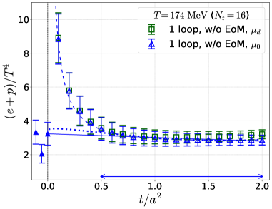
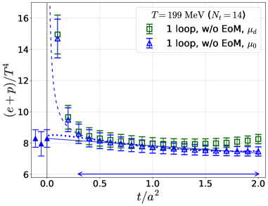
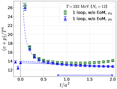
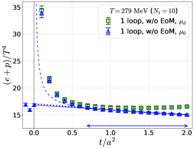
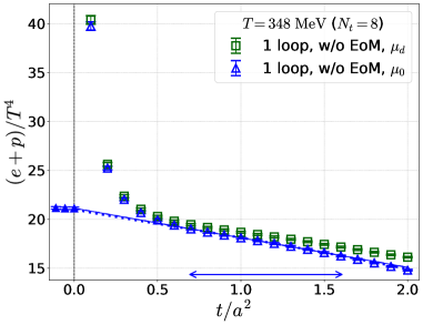
Figure 2: Entropy density $(\epsilon+p)/T^{4}$ with $\mu_{0}$ (blue) and $\mu_{d}$ (green) scales as function of the flow-time. One-loop matching coefficients of Ref. Makino:2014taa are used. Also shown are the results of the $t\to 0$ extrapolations using the data with the $\mu_{0}$-scale: Solid line is the linear fit using the linear window indicated by the arrow at the bottom of each plot, and the symbol at $t/a^{2}=0$ is the result of the linear fit for the physical entropy density in the $t\to 0$ limit. Fit results with the nonlinear ansatz (60) and linear+log ansatz (61) are shown by dashed and dotted curves together with the symbols at $t/a^{2}<0$ to the right and to the left, respectively. Errors are statistical only.

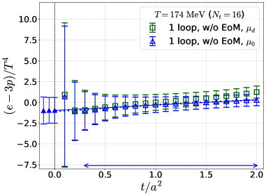
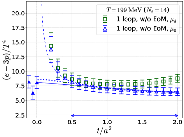
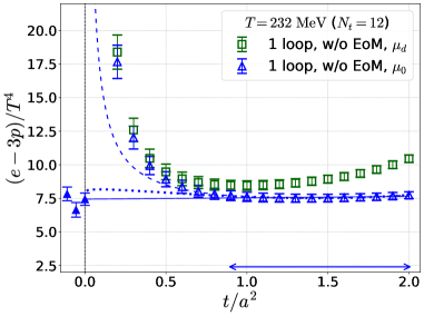
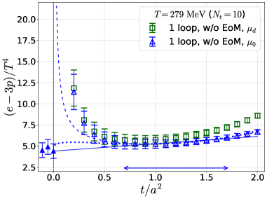
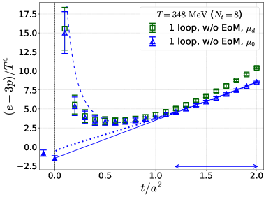
Figure 3: The same as Fig. 2 but for the trace anomaly $(\epsilon-3p)/T^{4}$.

Table 2: Results for EoS by the SFtX method with the $\mu_{0}$-scale using the one-loop matching coefficients of Ref. Makino:2014taa . The first parenthesis is for the statistical error, and the second for the systematic error due to the fit ansatz.

$T$[MeV]	$(\epsilon+p)/T^{4}$	$(\epsilon-3p)/T^{4}$	$\epsilon/T^{4}$	$p/T^{4}$
174	3.24(68)(${}^{+10}_{-1.19}$)	$-$0.96(1.56)(${}^{+00}_{-03}$)	2.27(65)(${}^{+06}_{-95}$)	1.10(43)(${}^{+03}_{-00}$)
199	8.30(57)(${}^{+00}_{-35}$)	8.09(1.03)(${}^{+13}_{-1.75}$)	8.25(56)(${}^{+03}_{-67}$)	$-$0.00(27)(${}^{+43}_{-02}$)
232	13.64(27)(${}^{+17}_{-1.15}$)	7.44(46)(${}^{+40}_{-80}$)	12.05(23)(${}^{+23}_{-1.14}$)	1.48(15)(${}^{+39}_{-05}$)
279	16.84(25)(${}^{+08}_{-92}$)	4.41(86)(${}^{+51}_{-00}$)	13.46(28)(${}^{+20}_{-1.29}$)	3.07(25)(${}^{+02}_{-15}$)
348	21.13(13)(${}^{+04}_{-00}$)	$-$1.49(35)(${}^{+68}_{-3.52}$)	15.91(12)(${}^{+00}_{-03}$)	4.87(20)(${}^{+21}_{-1.44}$)

Table 3: The same as the Table 2 but with the $\mu_{d}$-scale.

$T$[MeV]	$(\epsilon+p)/T^{4}$	$(\epsilon-3p)/T^{4}$	$\epsilon/T^{4}$	$p/T^{4}$
174	3.14(66)(${}^{+14}_{-1.41}$)	-1.15(1.70)(${}^{+10}_{-01}$)	2.14(65)(${}^{+09}_{-82}$)	1.14(43)(${}^{+02}_{-00}$)
199	8.22(56)(${}^{+34}_{-12}$)	7.80(1.04)(${}^{+88}_{-03}$)	8.02(54)(${}^{+77}_{-02}$)	0.10(26)(${}^{+00}_{-17}$)
232	13.45(27)(${}^{+1.13}_{-00}$)	7.43(52)(${}^{+1.86}_{-00}$)	12.03(24)(${}^{+96}_{-00}$)	1.53(15)(${}^{+00}_{-19}$)
279	16.19(24)(${}^{+1.31}_{-00}$)	4.76(99)(${}^{+05}_{-59}$)	13.38(31)(${}^{+12}_{-03}$)	3.06(26)(${}^{+06}_{-13}$)
348	21.25(13)(${}^{+00}_{-04}$)	2.36(75)(${}^{+91}_{-4.63}$)	15.57(12)(${}^{+14}_{-34}$)	4.92(20)(${}^{+28}_{-1.54}$)

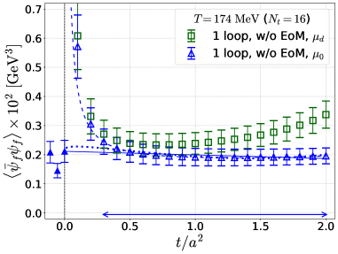
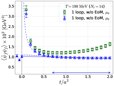
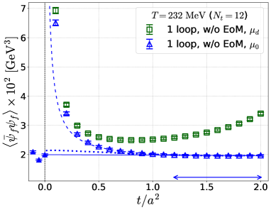
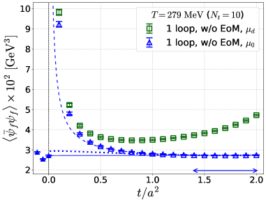
Figure 4: The same as Fig. 2 but for the chiral condensate $\left\langle\{\bar{\psi}_{f}\psi_{f}\}\right\rangle$ for $f=u$ or $d$ with VEV subtraction. The vertical axis is in units of GeV³.

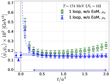
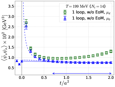
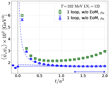
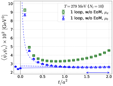
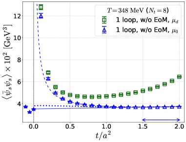
Figure 5: The same as Fig. 4 but for the $s$ quark ($f=s$).

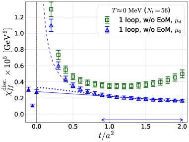
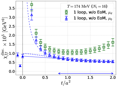
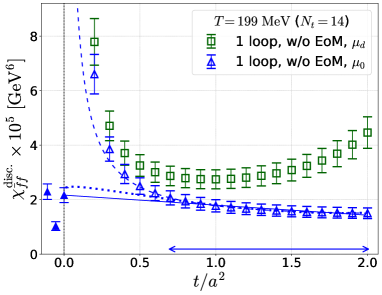
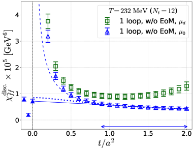
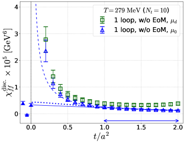
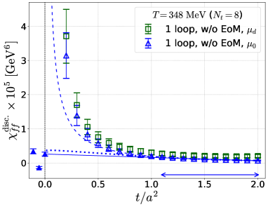
Figure 6: The same as Fig. 2 but for the disconnected chiral susceptibility $\chi_{\bar{f}f}^{\mathrm{disc.}}$ in the $\overline{\textrm{MS}}$-scheme at 2 GeV for $f=u$ or $d$ quark. The vertical axis is in units of GeV⁶.

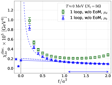
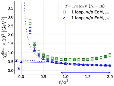
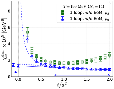
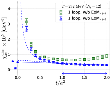
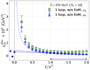
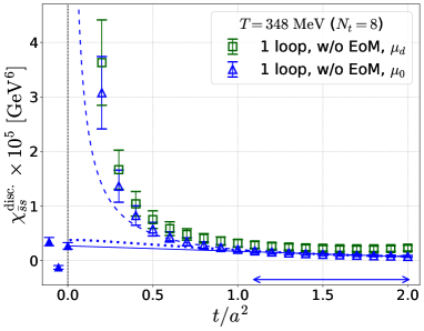
Figure 7: The same as Fig. 6 but for the $s$ quark.

Table 4: Results for chiral condensates and disconnected chiral susceptibilities by the SFtX method with the $\mu_{0}$-scale using the one-loop matching coefficients of Ref. Makino:2014taa . The chiral condensates are in units of GeV³, and the disconnected chiral susceptibilities are in units of GeV⁶. The first parenthesis is for the statistical error, and the second for the systematic error due to the fit ansatz.

$T$[MeV]	$\left\langle\{\bar{\psi}_{u}\psi_{u}\}(x)\right\rangle\times 10^{2}$	$\left\langle\{\bar{\psi}_{s}\psi_{s}\}(x)\right\rangle\times 10^{2}$	$\chi_{\bar{u}u}^{\mathrm{disc.}}\times 10^{5}$	$\chi_{\bar{s}s}^{\mathrm{disc.}}\times 10^{5}$
174	0.21(4)(${}^{+0}_{-7}$)	0.15(3)(${}^{+0}_{-5}$)	0.84(11)(${}^{+08}_{-54}$)	0.49(6)(${}^{+06}_{-37}$)
199	1.02(6)(${}^{+03}_{-18}$)	0.81(5)(${}^{+03}_{-14}$)	2.16(28)(${}^{+13}_{-1.14}$)	1.32(17)(${}^{+11}_{-75}$)
232	2.00(3)(${}^{+11}_{-18}$)	1.68(3)(${}^{+10}_{-12}$)	0.72(8)(${}^{+08}_{-53}$)	0.51(5)(${}^{+07}_{-41}$)
279	2.72(3)(${}^{+17}_{-18}$)	2.51(3)(${}^{+18}_{-10}$)	0.33(6)(${}^{+07}_{-38}$)	0.30(5)(${}^{+07}_{-36}$)
348	3.40(4)(${}^{+23}_{-26}$)	3.52(3)(${}^{+24}_{-26}$)	0.26(6)(${}^{+08}_{-40}$)	0.27(6)(${}^{+08}_{-40}$)

Results for the chiral condensate $\left\langle\{\bar{\psi}_{f}\psi_{f}\}\right\rangle$ for $f=u$ or $d$ quark and for $s$ quark are shown in Figs. 4 and 5, respectively, where the VEV’s are subtracted from the chiral condensates to remove singularities like $m^{2}/t$ Hieda:2016lly ; Taniguchi:2016ofw . Figures 6 and 7 show the results for the disconnected chiral susceptibility,

$$\chi_{\bar{f}f}^{\mathrm{disc.}}=\left\langle\left[\frac{1}{N_{\Gamma}}\sum_{x}\{\bar{\psi}_{f}\psi_{f}\}(x)\right]^{2}\right\rangle_{\!\mathrm{disc.}}-\left[\left\langle\frac{1}{N_{\Gamma}}\sum_{x}\{\bar{\psi}_{f}\psi_{f}\}(x)\right\rangle\right]^{2},$$ (68)

where connected quark loop contribution is dropped from the scalar density two-point function and $N_{\Gamma}$ is the lattice volume. Here, because the VEV-subtraction is not required for $\chi_{\bar{f}f}^{\mathrm{disc.}}$, we also study the case of $T=0$.

We find that, though a linear window is sometimes not clear with the conventional $\mu_{d}$-scale, the linear behavior is much improved by adopting the $\mu_{0}$-scale in particular at large $t/a^{2}$. The $\mu_{0}$-scale extends the applicability of the $t\to 0$ extrapolation method based on the linear window. In the followings, we perform $t\to 0$ extrapolations with the $\mu_{0}$-scale only.

In Figs. 4, 5, 6, and 7, the arrow at the bottom of each plot is the linear window we adopt, and the symbols at $t\sim 0$ shows the results of $t\to 0$ extrapolations, from the right to the left, using linear, nonlinear, and linear+log fits, respectively. In Table 4, we summarize the final results for the chiral condensates and disconnected chiral susceptibilities, obtained in the $t\to 0$ limit using the one-loop matching coefficients of Ref. Makino:2014taa with the $\mu_{0}$-scale.

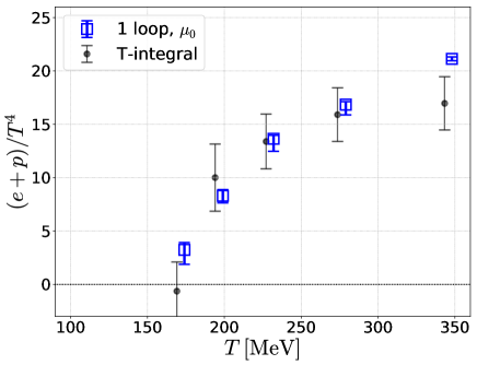
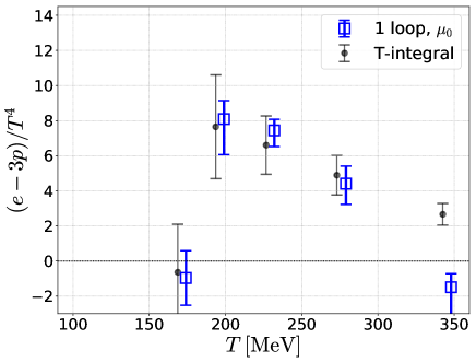
Figure 8: Results of the SFtX method for EoS with the $\mu_{0}$-scale as function of temperature. One-loop matching coefficients of Ref. Makino:2014taa are used. Black circles are the results of the $T$-integration method Umeda:2012er . Left panel: entropy density. Right panel: trace anomaly. Errors include systematic error due to the fit ansatz for the $t\to 0$ extrapolation. The symbols are slightly shifted horizontally to avoid overlapping.

IV.2 Results with the $\mu_{0}$-scale using one-loop matching coefficients

In Fig. 8, we summarize the physical results for EoS as function of temperature, obtained by $t\to 0$ extrapolations of the data with the $\mu_{0}$-scale shown in Sec. IV.1. The central values are taken from the linear fits and difference with the results of nonlinear and linear+log fits are taken as estimates of the systematic error due to the fit ansatz for the $t\to 0$ extrapolation.

Black dots in Fig. 8 show the results of EoS obtained previously by the conventional $T$-integration method using the same configurations Umeda:2012er . Our conclusions are the same as Ref. Taniguchi:2016ofw : At $T\mathrel{\hbox to0.0pt{\raise 2.20013pt\hbox{$<$}\hss}{\lower 2.20013pt\hbox{$\sim$}}}279$ MeV ($N_{t}\geq 10$), the SFtX method leads to EoS which is well consistent with the result of the conventional method, while $a$-independent lattice artifacts of $O\!\left((aT)^{2}=1/N_{t}^{2}\right)$ are suggested for $N_{t}\mathrel{\hbox to0.0pt{\raise 2.20013pt\hbox{$<$}\hss}{\lower 2.20013pt\hbox{$\sim$}}}8$. Because the continuum extrapolation is not taken yet, the good agreement of different estimations at $N_{t}\geq 10$ suggests that the remaining $O(a^{2}T^{2},\;a^{2}m^{2},\;a^{2}\Lambda_{\mathrm{QCD}}^{2})$ lattice artifacts are small with our lattice action at $a\simeq 0.07$ fm.

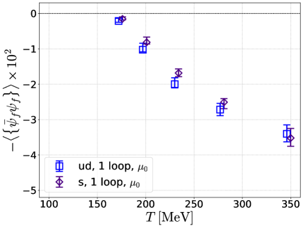
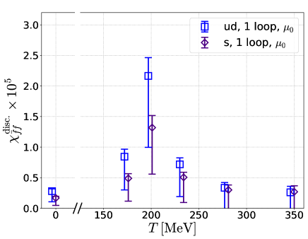
Figure 9: Results of the SFtX method with the $\mu_{0}$-scale for the VEV-subtracted chiral condensates $\left\langle\{\bar{\psi}_{f}\psi_{f}\}\right\rangle$ and disconnected chiral susceptibilities $\chi_{\bar{f}f}^{\mathrm{disc.}}$ in the $\overline{\textrm{MS}}$-scheme at 2 GeV, as function of temperature. One-loop matching coefficients of Ref. Makino:2014taa are used. Left panel: $-\left\langle\{\bar{\psi}_{f}\psi_{f}\}\right\rangle$ with the vertical axis in units of GeV³. Following a convention, we plot $-\left\langle\{\bar{\psi}_{f}\psi_{f}\}\right\rangle$. Right panel: $\chi_{\bar{f}f}^{\mathrm{disc.}}$ with the vertical axis in units of GeV⁶. Errors include systematic error due to the fit ansatz for the $t\to 0$ extrapolation. The symbols are slightly shifted horizontally to avoid overlapping.

Results for the VEV-subtracted chiral condensates are shown in the left panel of Fig. 9. In the right panel of Fig. 9, we show the results for disconnected chiral susceptibilities as function of temperature. Because the VEV-subtraction has no effects in this quantity, we also show the results at $T=0$. We find a clear peak at $T\simeq 199$ MeV, which may be indicating the pseudocritical point around $T_{\mathrm{pc}}\sim 190$ MeV previously suggested using the Polyakov loop etc. Umeda:2012er . We also note that, although the errors are large yet, the height of the peak looks increasing as we decrease the valence quark mass from $s$ quark to $u$ (or $d$) quark.

V Test of two-loop matching coefficients

We now test the effects of two-loop matching coefficients for EMT by Harlander et al. Harlander:2018zpi in QCD with $2+1$ flavors of dynamical quarks. Following the discussion in Sec. IV, we adopt the $\mu_{0}$-scale in this test. As mentioned in Sec. I, unlike the one-loop coefficients of Ref. Makino:2014taa , the EoM is used in the two-loop coefficients of Refs. Harlander:2018zpi .

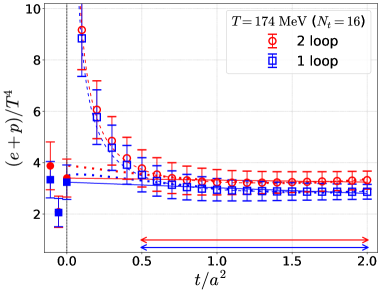
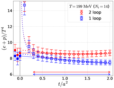
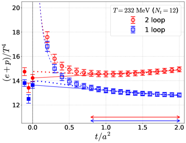
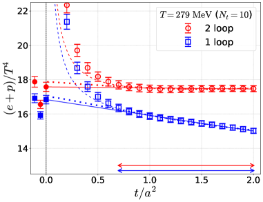
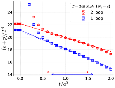
Figure 10: Entropy density $(\epsilon+p)/T^{4}$ with the $\mu_{0}$-scale as function of the flow-time. Results using one-loop matching coefficients of Ref. Makino:2014taa are compared with those using two-loop matching coefficients of Ref. Harlander:2018zpi . The arrows at the bottom indicate the linear windows at each temperature. Symbols at $t/a^{2}=0$ and solid lines with the same color are the results of the linear fits. Fit results with the nonlinear ansatz (60) and linear+log ansatz (61) or (62) are shown by dashed and dotted curves together with the symbols at $t/a^{2}<0$ to the right and to the left, respectively. Errors are statistical only.

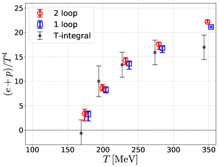
Figure 11: Results of the SFtX method for the entropy density $(\epsilon+p)/T^{4}$ with the $\mu_{0}$-scale, as function of temperature. Results using one-loop matching coefficients of Ref. Makino:2014taa without using the EoM are compared with results using two-loop matching coefficients of Ref. Harlander:2018zpi in which the EoM is used. Black dots are the results of the $T$-integration method Umeda:2012er . Errors include systematic error due to the fit ansatz for the $t\to 0$ extrapolation. The symbols are slightly shifted horizontally to avoid overlapping.

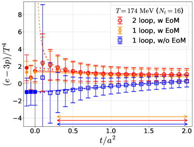
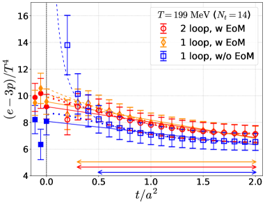
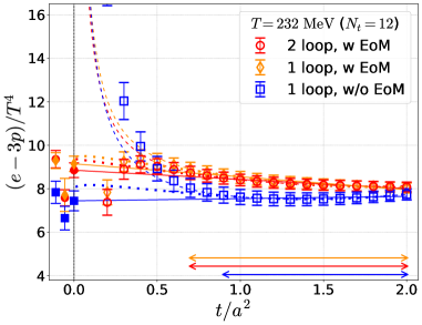
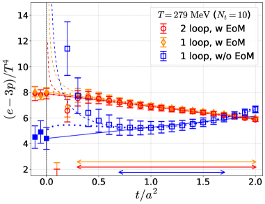
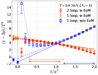
Figure 12: The same as Fig. 10 but for the trace anomaly $(\epsilon-3p)/T^{4}$. Also shown are the results using one-loop part of the matching coefficients of Ref. Harlander:2018zpi in which the EoM is used.

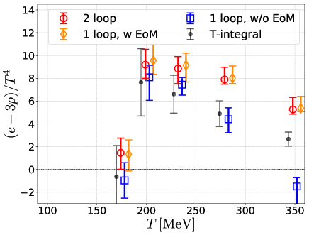
Figure 13: Results of the SFtX method for the trace anomaly $(\epsilon-3p)/T^{4}$ with the $\mu_{0}$-scale, as function of temperature. Results using one-loop matching coefficients of Ref. Makino:2014taa without using the EoM are compared with results using two-loop matching coefficients of Ref. Harlander:2018zpi in which the EoM is used. Also shown are the results using one-loop part of the matching coefficients of Ref. Harlander:2018zpi in which the EoM is used. Black dots are the results of the $T$-integration method Umeda:2012er . Errors include systematic error due to the fit ansatz for the $t\to 0$ extrapolation. The symbols are slightly shifted horizontally to avoid overlapping.

V.1 Entropy density

In Fig. 10, we compare the results of the entropy density at finite $t$ using the one-loop matching coefficients of Ref. Makino:2014taa (blue squares) and those using the two-loop coefficients of Ref. Harlander:2018zpi (red circles). Note that, because the contribution of the EoM to the EMT given by Eq. (31) is proportional to $\delta_{\mu\nu}$, only the trace part of the EMT is affected by the use of the EoM. Thus, the EoM has no effects in the entropy density which is a trace-less combination of the EMT. We find that the entropy density with the two-loop coefficients is larger than its one-loop value at finite $t$, but the difference becomes smaller in the $t\to 0$ limit.

In the previous test in quenched QCD, it was reported that the use of two-loop matching coefficients generally makes the data flatter in the flow-time $t$ and thus makes the $t\to 0$ extrapolation more stable Iritani2019 . In our study, we find in Fig. 10 that, though a similar general tendency may be visible, we do not see an apparent improvement in the $t\to 0$ extrapolation with the use of two-loop coefficients. This is caused by the fact that we have sufficiently wide linear windows for $t\to 0$ extrapolation with the one-loop coefficients — no much room was left for drastic improvement on our fine lattice. Two-loop matching coefficients may help a study of other observables or on coarser lattices.

Physical results for the entropy density with one- and two-loop matching coefficients are shown in Fig. 11. The errors include the systematic error due to the $t\to 0$ extrapolation. Here, it should be recalled that EMT data at $T\mathrel{\hbox to0.0pt{\raise 2.20013pt\hbox{$>$}\hss}{\lower 2.20013pt\hbox{$\sim$}}}348$ MeV are contaminated with $O\!\left((aT)^{2}=1/N_{t}^{2}\right)$ lattice artifacts at $N_{t}\mathrel{\hbox to0.0pt{\raise 2.20013pt\hbox{$<$}\hss}{\lower 2.20013pt\hbox{$\sim$}}}8$ Taniguchi:2016ofw . We find that one- and two-loop results agree well within the errors at $T<279$ MeV ($N_{t}>10$).

V.2 Trace anomaly

In Fig. 12, we show the results for the trace anomaly $(\epsilon-3p)/T^{4}$ as function of the flow-time. The trace anomaly is just the trace part of the EMT and thus will be sensitively affected by the EoM on finite lattices. In order to identify the effects of EoM clearly, we also compute the trace anomaly using the one-loop part of the matching coefficients of Ref. Harlander:2018zpi in which the EoM is used. We find that one- and two-loop results both using the EoM are close with each other, while the one-loop results without using the EoM deviates from the results using the EoM. We thus conclude that the deviation is mainly due to the use of the EoM. The deviation increases with increasing $T$ (decreasing $N_{t}$) and becomes sizable at high temperatures, $T\mathrel{\hbox to0.0pt{\raise 2.20013pt\hbox{$>$}\hss}{\lower 2.20013pt\hbox{$\sim$}}}279$ MeV ($N_{t}\mathrel{\hbox to0.0pt{\raise 2.20013pt\hbox{$<$}\hss}{\lower 2.20013pt\hbox{$\sim$}}}10$).

Physical results of the trace anomaly extracted by the $t\to 0$ extrapolation are summarized in Fig. 13. We find that though the analyses with and without using the EoM lead to consistent results within errors at low temperatures, they show visible discrepancy at high temperatures, $T\mathrel{\hbox to0.0pt{\raise 2.20013pt\hbox{$>$}\hss}{\lower 2.20013pt\hbox{$\sim$}}}279$ MeV ($N_{t}\mathrel{\hbox to0.0pt{\raise 2.20013pt\hbox{$<$}\hss}{\lower 2.20013pt\hbox{$\sim$}}}10$). Even with disregarding the data at $T\mathrel{\hbox to0.0pt{\raise 2.20013pt\hbox{$>$}\hss}{\lower 2.20013pt\hbox{$\sim$}}}348$ MeV $(N_{t}=8)$ where contamination of $O\!\left((aT)^{2}=1/N_{t}^{2}\right)$ lattice artifacts is suggested in EMT, we see discrepancy at $T\simeq 279$ MeV ($N_{t}=10$). The $O\!\left((aT)^{2}\right)$ lattice artifacts will contaminate the EoM too. Our results suggest that the EoM suffers from larger $O\!\left((aT)^{2}=1/N_{t}^{2}\right)$ discretization errors than the EMT, and has visible effect at $N_{t}\mathrel{\hbox to0.0pt{\raise 2.20013pt\hbox{$<$}\hss}{\lower 2.20013pt\hbox{$\sim$}}}10$.

Final results for EoS extracted by the $t\to 0$ extrapolation with the $\mu_{0}$-scale are summarized in Tables 2, 5 and 6.

Table 5: Results for EoS by the SFtX method with the $\mu_{0}$-scale using the two-loop matching coefficients of Ref. Harlander:2018zpi . The first parenthesis is for the statistical error, and the second for the systematic error due to the fit ansatz.

$T$[MeV]	$(\epsilon+p)/T^{4}$	$(\epsilon-3p)/T^{4}$	$\epsilon/T^{4}$	$p/T^{4}$
174	3.40(75)(${}^{+48}_{-1.32}$)	1.46(1.24)(${}^{+38}_{-75}$)	2.90(60)(${}^{+44}_{-1.22}$)	0.57(39)(${}^{+10}_{-00}$)
199	8.67(61)(${}^{+37}_{-24}$)	9.18(93)(${}^{+1.00}_{-00}$)	8.81(56)(${}^{+45}_{-00}$)	$-$0.12(26)(${}^{+00}_{-13}$)
232	14.22(29)(${}^{+53}_{-81}$)	8.85(34)(${}^{+51}_{-1.28}$)	12.86(24)(${}^{+52}_{-99}$)	1.38(12)(${}^{+04}_{-00}$)
279	17.58(27)(${}^{+30}_{-1.03}$)	7.89(40)(${}^{+01}_{-09}$)	15.14(22)(${}^{+20}_{-75}$)	2.44(12)(${}^{+11}_{-00}$)
348	22.16(14)(${}^{+00}_{-01}$)	5.26(34)(${}^{+00}_{-23}$)	18.00(13)(${}^{+00}_{-06}$)	4.03(06)(${}^{+04}_{-73}$)

Table 6: Results for EoS by the SFtX method with the $\mu_{0}$-scale using the one-loop part of the matching coefficients of Ref. Harlander:2018zpi . The first parenthesis is for the statistical error, and the second for the systematic error due to the fit ansatz.

$T$[MeV]	$(\epsilon+p)/T^{4}$	$(\epsilon-3p)/T^{4}$	$\epsilon/T^{4}$	$p/T^{4}$
174	3.24(68)(${}^{+10}_{-1.19}$)	1.33(1.27)(${}^{+00}_{-75}$)	2.75(56)(${}^{+07}_{-1.13}$)	0.56(39)(${}^{+01}_{-00}$)
199	8.30(57)(${}^{+00}_{-35}$)	9.56(96)(${}^{+1.01}_{-09}$)	8.55(52)(${}^{+02}_{-11}$)	$-$0.30(26)(${}^{+01}_{-13}$)
232	13.64(27)(${}^{+17}_{-1.15}$)	9.14(35)(${}^{+16}_{-1.44}$)	12.50(23)(${}^{+17}_{-1.26}$)	1.16(12)(${}^{+01}_{-00}$)
279	16.84(25)(${}^{+08}_{-92}$)	8.01(36)(${}^{+03}_{-32}$)	14.61(21)(${}^{+07}_{-76}$)	2.25(11)(${}^{+02}_{-00}$)
348	21.13(13)(${}^{+04}_{-00}$)	5.37(29)(${}^{+49}_{-00}$)	17.26(12)(${}^{+03}_{-00}$)	3.85(05)(${}^{+01}_{-75}$)

VI Conclusions

We presented the results of our tests of the $\mu_{0}=e^{-\gamma_{E}/2}/\sqrt{2t}$ renormalization scale and two-loop matching coefficients recently calculated by Harlander et al. Harlander:2018zpi . For this test, we revisited the case of QCD with heavy u and d quarks Taniguchi:2016ofw .

We find that, comparing with the results using the conventional $\mu_{d}=1/\sqrt{8t}$ scale, the $\mu_{0}$-scale improves the quality of perturbative expressions, in particular at large $t$, and thus leads to clearer and wider linear windows so that we can carry out $t\to 0$ extrapolations much confidently. We also find that, for observables for which the linear window is clear with the conventional $\mu_{d}$-scale, the results using $\mu_{0}$- and $\mu_{d}$-scales are consistent with each other, i.e., the results extrapolated to the $t\to 0$ limit are insensitive to the choice of the renormalization scale, as expected.

Concerning the test of two-loop matching coefficients, unlike the case of the one-loop matching coefficients of Ref. Makino:2014taa , the equation of motion for quark fields in the continuum limit is used by Harlander et al. in their calculation of the two-loop matching coefficients Harlander:2018zpi . For the entropy density in which the equation of motion has no effects, we found that the results using the two-loop coefficients are well consistent with the results using one-loop coefficients. On the other hand, for the trace anomaly in which the equation of motion does affect, we found discrepancies between the one- and two-loop results at high temperatures (small $N_{t}$’s). The main origin of the discrepancies was identified as the use of equation of motion by a direct comparison of the results of one-loop coefficients with and without using the equation of motion. Our results suggest that the equation of motion suffers from large $O\!\left((aT)^{2}\right)=O\!\left(1/N_{t}^{2}\right)$ discretization error at $N_{t}\mathrel{\hbox to0.0pt{\raise 2.20013pt\hbox{$<$}\hss}{\lower 2.20013pt\hbox{$\sim$}}}10$. Therefore, one should be cautious when extracting physical quantities such as the trace anomaly which are affected by the use of the equation of motion. This point is not, however, the problem of the two-loop coefficients themselves, and as our results illustrate this point should be regarded as a more general problem caused by discretization errors.

We are attempting to extend applications of the SFtX method in various directions: thermodynamics of $2+1$ flavor QCD at the physical point Lat2017-kanaya ; Lat2019-kanaya , shear and bulk viscosities from two-point correlation functions of the energy-momentum tensor Taniguchi:2017ibr , end-point of first-order deconfining transition region in QCD near the quenched limit Shirogane , PCAC quark masses ABaba , etc. The choice of the $\mu_{0}$-scale as well as higher order coefficients may help improving these calculations too.

Appendix A Group factors

We normalize the gauge group generators as

$$\textrm{tr}\left(T^{a}T^{b}\right)=-\frac{1}{2}\delta^{ab}.$$ (69)

The structure constant defined by $[T^{a},T^{b}]=f^{abc}T^{c}$ has quadratic Casimirs as

$$f^{acd}f^{bcd}=C_{2}(G)\,\delta^{ab},\qquad T^{a}T^{a}=-C_{2}(R)\,\textbf{1}.$$ (70)

In the perturbative expressions in Sec. II.2, group factors are defined by

$$C_{\!A}\equiv C_{2}(G),\qquad T_{F}\equiv T(R)\,N_{f},\qquad C_{F}\equiv C_{2}(R).$$ (71)

For $G=SU(N)$ and $R=N$,

$$C_{\!A}=N,\qquad T_{F}=\frac{1}{2}N_{f},\qquad C_{F}=\frac{N^{2}-1}{2N}.$$ (72)

In particular, for the $N_{f}=2+1$ QCD,

$$C_{\!A}=3,\qquad T_{F}=\frac{3}{2},\qquad C_{F}=\frac{4}{3},$$ (73)

and for the quenched QCD (the $SU(3)$ pure Yang–Mills)

$$C_{\!A}=3,\qquad T_{F}=0,\qquad C_{F}=0.$$ (74)

Appendix B Consistency of matching coefficients

In this appendix, we confirm that the matching coefficients of Refs. Makino:2014taa and Harlander:2018zpi for EMT are consistent with each other.

B.1 One-loop confirmation

We confirm that Eqs. (42)–(55) restricted to the one-loop level is consistent with the results of Ref. Makino:2014taa .

One way to see this is to construct the small flow time expansion of the “reduced EMT” in Eq. (32). Using the matrix $\zeta(t)$ defined by

$$\tilde{\mathcal{O}}_{i\mu\nu}(t,x)=\zeta_{ij}(t)\,\mathcal{O}_{j\mu\nu}(x)+O(t),$$ (75)

the coefficients $\tilde{c}_{i}(t)$ in

$$T_{\mu\nu}(x)$$

$$=\tilde{c}_{1}(t)\tilde{\mathcal{O}}_{1,\mu\nu}(t,x)+\tilde{c}_{2}(t)\tilde{\mathcal{O}}_{2,\mu\nu}(t,x)+\tilde{c}_{3}(t)\tilde{\mathcal{O}}_{3,\mu\nu}(t,x)+\tilde{c}_{4}(t)\tilde{\mathcal{O}}_{4,\mu\nu}(t,x)+\tilde{c}_{5}(t)\tilde{\mathcal{O}}_{5,\mu\nu}(t,x)$$

$$\qquad{}+O(t),$$ (76)

where the left-hand side is Eq. (32), are given by

$$\tilde{c}_{i}(t)=\frac{1}{g_{0}^{2}}\left\{\left(\zeta^{-1}\right)_{1i}(t)-\frac{1}{4}\left(\zeta^{-1}\right)_{2i}(t)\right\}+\frac{1}{4}\left(\zeta^{-1}\right)_{3i}(t).$$ (77)

Compare this to Eq. (4.16) of Ref. Makino:2014taa . The one-loop $\zeta(t)$ obtained in Ref. Makino:2014taa then yields

$$\tilde{c}_{1}(t) =\frac{1}{g^{2}}\left\{1+\frac{g^{2}}{(4\pi)^{2}}\left[-\beta_{0}L(\mu,t)-\frac{7}{3}C_{\!A}+\frac{3}{2}T_{F}\right]\right\},$$ (78)

$$\tilde{c}_{2}(t) =\frac{1}{4g^{2}}\left\{-1+\frac{g^{2}}{(4\pi)^{2}}\left[\beta_{0}L(\mu,t)+\frac{25}{6}C_{\!A}-3T_{F}\right]\right\},$$ (79)

$$\tilde{c}_{3}(t) =\frac{1}{4}\left[1+\frac{g^{2}}{(4\pi)^{2}}C_{F}\left(\frac{3}{2}+\ln 432\right)\right],$$ (80)

$$\tilde{c}_{4}(t) =\frac{g^{2}}{(4\pi)^{2}}C_{F}\left(-\frac{1}{4}\right),$$ (81)

$$\tilde{c}_{5}(t) =\frac{g^{2}}{(4\pi)^{2}}C_{F}\left(-\frac{3}{2}\right).$$ (82)

Note that $\tilde{c}_{4}(t)$ and $\tilde{c}_{5}(t)$ are one-loop quantities because Eq. (32) does not contain $\mathcal{O}_{4,\mu\nu}(x)$ and $\mathcal{O}_{5,\mu\nu}(x)$ and $\tilde{\mathcal{O}}_{4,\mu\nu}(t,x)$ and $\tilde{\mathcal{O}}_{5,\mu\nu}(t,x)$ appear only through loop diagrams. To translate these coefficients $\tilde{c}_{i}(t)$ in Eq. (76) to the coefficients in Eq. (41), we have to eliminate the operator $\tilde{\mathcal{O}}_{5,\mu\nu}(t,x)$ from Eq. (76) in favor of $\tilde{\mathcal{O}}_{4,\mu\nu}(t,x)$ and $\tilde{\mathcal{O}}_{2,\mu\nu}(t,x)$ by using the relation (36). In the present order of approximation, this is easy because we can use the relation

$$\frac{1}{2}\tilde{\mathcal{O}}_{4,\mu\nu}(t,x)+\tilde{\mathcal{O}}_{5.\mu\nu}(t,x)=0$$ (83)

that holds in the tree-level in Eq. (76) because $\tilde{c}_{4}(t)$ and $\tilde{c}_{5}(t)$ are already one-loop quantities. After this elimination, we have

$$\check{c}_{1}(t) =\tilde{c}_{1}(t),$$ (84)

$$\check{c}_{2}(t) =\tilde{c}_{2}(t),$$ (85)

$$\mathring{\check{c}}_{3}(t) =\tilde{c}_{3}(t),$$ (86)

$$\mathring{\check{c}}_{4}(t) =\tilde{c}_{4}(t)-\frac{1}{2}\tilde{c}_{5}(t).$$ (87)

We see that these precisely coincide with Eqs. (42), (43), (54), and (55) in the one-loop level.

Another way to see the consistency is the following. The one-loop result of Ref. Makino:2014taa (cf. Eqs. (4.60)–(4.64)) gives, for the coefficients in Eq. (24),

$$c_{1}^{\text{old}}(t) =\frac{1}{g^{2}}\left\{1+\frac{g^{2}}{(4\pi)^{2}}\left[-\beta_{0}L(\mu,t)-\frac{7}{3}C_{\!A}+\frac{3}{2}T_{F}\right]\right\},$$ (88)

$$c_{2}^{\text{old}}(t) =\frac{1}{4g^{2}}\frac{g^{2}}{(4\pi)^{2}}\left(\frac{11}{6}C_{\!A}+\frac{11}{6}T_{F}\right),$$ (89)

$$c_{3}^{\text{old}}(t) =\frac{1}{4}\left[1+\frac{g^{2}}{(4\pi)^{2}}C_{F}\left(\frac{3}{2}+\ln 432\right)\right],$$ (90)

$$c_{4}^{\text{old}}(t) =\frac{g^{2}}{(4\pi)^{2}}\frac{3}{4}C_{F},$$ (91)

$$c_{5}^{\text{old}}(t) =-\left\{1+\frac{g^{2}}{(4\pi)^{2}}C_{F}\left[3L(\mu,t)+\frac{7}{2}+\ln 432\right]\right\}.$$ (92)

They differ from the coefficients obtained from Eq. (41):

$$c_{1}(t) =\check{c}_{1}(t)=\frac{1}{g^{2}}\left\{1+\frac{g^{2}}{(4\pi)^{2}}\left[-\beta_{0}L(\mu,t)-\frac{7}{3}C_{\!A}+\frac{3}{2}T_{F}\right]\right\},$$ (93)

$$c_{2}(t) =\check{c}_{2}(t)+\frac{1}{4}\check{c}_{1}(t)=\frac{1}{4g^{2}}\frac{g^{2}}{(4\pi)^{2}}\left(\frac{11}{6}C_{\!A}-\frac{3}{2}T_{F}\right),$$ (94)

$$c_{3}(t) =\mathring{\check{c}}_{3}(t)=\frac{1}{4}\left[1+\frac{g^{2}}{(4\pi)^{2}}C_{F}\left(\frac{3}{2}+\ln 432\right)\right],$$ (95)

$$c_{4}(t) =\mathring{\check{c}}_{4}(t)+2\mathring{\check{c}}_{3}(t)=\frac{1}{2}\left[1+\frac{g^{2}}{(4\pi)^{2}}C_{F}\left(\frac{5}{2}+\ln 432\right)\right],$$ (96)

$$c_{5}(t) =0.$$ (97)

These differences arise from the backreaction of the elimination of $\tilde{\mathcal{O}}_{5\mu\nu}(t,x)$. Inserting $\tilde{\mathcal{O}}_{5,\mu\nu}=-\mathring{d}_{5}^{-1}d_{2}\tilde{\mathcal{O}}_{2,\mu\nu}-\mathring{d}_{5}^{-1}\mathring{d}_{4}\tilde{\mathcal{O}}_{4,\mu\nu}$ [see Eq. (36)] into Eq. (24) with the old coefficients (88)–(92) to eliminate $c_{5}^{\text{old}}\tilde{\mathcal{O}}_{5,\mu\nu}$, we confirm that the old coefficients (88)–(92) precisely reproduce the new coefficients (93)–(96).

B.2 Two-loop confirmation

As pointed out in Ref. Suzuki:2013gza , in the case of the pure Yang-Mills theory, a certain part of the two-loop order coefficients can be extracted by using the trace anomaly without any higher order calculations. The expression in our present notation is (see Eq. (4.69) of Ref. Makino:2014taa ),

$$c_{2}(t)\equiv\check{c}_{2}(t)+\frac{1}{4}\check{c}_{1}(t)=\frac{1}{4g^{2}}\left[\frac{g^{2}}{(4\pi)^{2}}\frac{\beta_{0}}{2}+\frac{g^{4}}{(4\pi)^{4}}\left(\frac{\beta_{1}}{2}-\frac{7}{4}C_{\!A}\beta_{0}\right)\right],$$ (98)

where the second term in the right-hand side contains the information in the two-loop order. This coincides with the result obtained from Eqs. (42) and (43) for the pure Yang-Mills theory.

We can similarly deduce three-loop $c_{2}(t)$ for the pure Yang-Mills theory from the two-loop coefficients. A concrete form is given in Ref. Iritani2019 .

Appendix C Alternative method for flowed fermionic bilinear observables

As discussed in Appendix A of Ref. Taniguchi:2016ofw , fermionic parts of the EMT are given in terms of

$$t_{\mu\nu}^{f}(t) \equiv\frac{1}{N_{\Gamma}}\sum_{x}\left\langle\bar{\chi}_{f}(t,x)\,\gamma_{\mu}\left(D_{\nu}-\overleftarrow{D}_{\nu}\right)\chi_{f}(t,x)\right\rangle$$

$$=-\frac{1}{N_{\Gamma}}\sum_{x,v,w}\Biggl{\{}\left\langle\sum_{\alpha,i}\left[\gamma_{\mu}D_{\nu}^{x}K(t,x;0,v)S_{f}(v,w)K(t,x;0,w)^{\dagger}\right]_{\alpha i,\alpha i}\right\rangle$$

$$\qquad\qquad\qquad\qquad{}-\left\langle\sum_{\alpha,i}\left[K(t,x;0,v)S_{f}(v,w)K(t,x;0,w)^{\dagger}\overleftarrow{D}_{\nu}^{x}\gamma_{\mu}\right]_{\alpha i,\alpha i}\right\rangle\Biggr{\}},$$ (99)

and

$$s^{f}(t) \equiv\frac{1}{N_{\Gamma}}\sum_{x}\left\langle\bar{\chi}_{f}(t,x)\,\chi_{f}(t,x)\right\rangle$$

$$=-\frac{1}{N_{\Gamma}}\sum_{x,v,w}\left\langle\sum_{\alpha,i}\left\{K(t,x;0,v)\left[S_{f}(v,w)-c_{\mathrm{fl}}\,\delta_{v,w}\right]K(t,x;0,w)^{\dagger}\right\}_{\alpha i,\alpha i}\right\rangle,$$ (100)

where the covariant derivatives in Eq. (99) refer to the flowed gauge field $B_{\mu}(t,x)$, $N_{\Gamma}=\sum_{x}$ is the number of lattice points, $\alpha$ and $i$ denote the spinor and color indices, respectively, and $c_{\mathrm{fl}}$ is an improvement coefficient associated with the flowed quark field Luscher:2013cpa . $S_{f}(x,y)$ is the quark propagator with the bare mass $m_{f0}$, and $K(t,x;s,y)$ is the fundamental solution to the flow equation defined by

$$\left(\partial_{t}-\Delta\right)K(t,x;s,y)=0,\qquad K(t,x;t,y)=\delta_{x,y}.$$ (101)

The dagger ($\dagger$) in Eqs. (99) and (100) implies the hermitian conjugation with respect to the gauge and spinor indices only. Note that $K$ and $D_{\nu}$ have no spinor indices. In Ref. Taniguchi:2016ofw , we have computed them by introducing noise vectors to evaluate the trace over space-time points in Eqs. (99) and (100). Expressions for other local fermionic bilinear operators can be written down similarly.

Here, we note that Eqs. (99) and (100) can be equally written as

$$t_{\mu\nu}^{r}(t) =-\frac{1}{N_{\Gamma}}\sum_{x,y,v,w}\Biggl{\{}\left\langle\sum_{\alpha,i}\left[K(t,x;0,y)^{\dagger}\gamma_{\mu}D_{\nu}^{x}K(t,x;0,v)S_{r}(v,w)\right]_{\alpha i,\alpha i}\delta_{w,y}\right\rangle$$

$$\qquad\qquad\qquad\qquad{}+\left\langle\delta_{y,w}\sum_{\alpha,i}\left[S_{r}(v,w)^{\dagger}K(t,x;0,v)^{\dagger}\overleftarrow{D}_{\nu}^{x}\gamma_{\mu}K(t,x;0,y)\right]_{\alpha i,\alpha i}\right\rangle\Biggr{\}},$$ (102)

where we have used the relation $S_{r}(v,w)=\gamma_{5}S_{r}(w,v)^{\dagger}\gamma_{5}$ , and

$$s^{r}(t)=-\frac{1}{N_{\Gamma}}\sum_{x,y,v,w}\left\langle\sum_{\alpha,i}\left\{K(t,x;0,y)^{\dagger}K(t,x;0,v)\left[S_{r}(v,w)-c_{\text{fl}}\delta_{v,w}\right]\right\}_{\alpha i,\alpha i}\delta_{w,y}\right\rangle.$$ (103)

We thus introduce a new noise field

$$\left\langle\eta_{\alpha i}(x)\right\rangle_{\eta}=0,\qquad\left\langle\eta_{\alpha i}(x)\eta_{\beta j}(y)^{*}\right\rangle_{\eta}=\delta_{\alpha\beta}\delta_{ij}\delta_{x,y},$$ (104)

and define

$$\Xi(t,x) \equiv \sum_{y}K(t,x;0,y)\,\eta(y),$$ (105)

$$Z_{r}(t,x) \equiv \sum_{v,w}K(t,x;0,v)\,S_{r}(v,w)\,\eta(w),$$ (106)

where contraction of spinor and color indices is understood. We then obtain compact expressions as

$$t_{\mu\nu}^{r}(t)=-\frac{1}{N_{\Gamma}}2\operatorname{Re}\left\langle\left\langle\sum_{x}\Xi(t,x)^{\dagger}\gamma_{\mu}D_{\nu}Z_{r}(t,x)\right\rangle_{\eta}\right\rangle,$$ (107)

where the gauge field in the covariant derivative $D_{\nu}$ is the flowed $B_{\mu}(t,x)$, and

$$s^{r}(t)=-\frac{1}{N_{\Gamma}}\left\langle\left\langle\sum_{x}\Xi(t,x)^{\dagger}Z_{r}(t,x)\right\rangle_{\eta}\right\rangle+c_{\text{fl}}\frac{1}{N_{\Gamma}}\left\langle\left\langle\sum_{x}\Xi(t,x)^{\dagger}\Xi(t,x)\right\rangle_{\eta}\right\rangle.$$ (108)

The building blocks obey the forward flow equations as

$$(\partial_{t}-\Delta)\Xi(t,x) =0, \Xi(0,x) =\eta(x),$$ (109)

$$(\partial_{t}-\Delta)Z_{r}(t,x) =0, Z_{r}(0,x) =\sum_{y}S_{r}(x,y)\eta(y),$$ (110)

which can be solved by the time-forward Runge–Kutta method as explained in Appendix D.2 of Ref. Luscher:2013cpa . That is, setting $\partial_{t}\chi_{t}=\Delta(V_{t})\chi_{t}$, the Runge–Kutta proceeds as

$$\phi_{0} =\chi_{t},$$

$$\phi_{1} =\phi_{0}+\frac{1}{4}\Delta_{0}\phi_{0},$$

$$\phi_{2} =\phi_{0}+\frac{8}{9}\Delta_{1}\phi_{1}-\frac{2}{9}\Delta_{0}\phi_{0},$$

$$\phi_{3} =\phi_{1}+\frac{3}{4}\Delta_{2}\phi_{2},$$ (111)

where

$$\Delta_{i}=\epsilon\Delta(W_{i}),\qquad i=0,1,2,$$ (112)

and

$$\chi_{t+\epsilon}=\phi_{3}+O(\epsilon^{4}).$$ (113)

These new representations are advantageous in the sense that they do not require the Runge–Kutta steps proceeding backward in the flow time (see Appendix B of Ref. Taniguchi:2016ofw ) which is numerically demanding.

References

- (1) R. Narayanan and H. Neuberger, “Infinite phase transitions in continuum Wilson loop operators,” J. High Energy Phys. 0603, 064 (2006).
- (2) M. Lüscher, “Trivializing maps, the Wilson flow and the HMC algorithm,” Commun. Math. Phys. 293, 899 (2010).
- (3) M. Lüscher, “Properties and uses of the Wilson flow in lattice QCD,” J. High Energy Phys. 1008, 071 (2010), Erratum: [JHEP 1403, 092 (2014)].
- (4) M. Lüscher and P. Weisz, “Perturbative analysis of the gradient flow in nonabelian gauge theories,” J. High Energy Phys. 1102, 051 (2011).
- (5) M. Lüscher, “Chiral symmetry and the Yang-Mills gradient flow,” J. High Energy Phys. 1304, 123 (2013).
- (6) M. Lüscher, “Future applications of the Yang-Mills gradient flow in lattice QCD,” Proc. Sci., LATTICE 2013, 016 (2014).
- (7) A. Ramos, “The Yang-Mills gradient flow and renormalization,” Proc. Sci., LATTICE 2014, 017 (2015).
- (8) H. Suzuki, “Energy-momentum tensor on the lattice: recent developments,” Proc. Sci., LATTICE 2016, 002 (2017).
- (9) H. Suzuki, “Energy-momentum tensor from the Yang-Mills gradient flow,” Prog. Theor. Exp. Phys. 2013, 083B03 (2013), Erratum: [PTEP 2015, 079201 (2015)].
- (10) H. Makino and H. Suzuki, “Lattice energy-momentum tensor from the Yang-Mills gradient flow—inclusion of fermion fields,” Prog. Theor. Exp. Phys. 2014, 063B02 (2014), Erratum: [PTEP 2015, 079202 (2015)].
- (11) T. Endo, K. Hieda, D. Miura and H. Suzuki, “Universal formula for the flavor nonsinglet axial-vector current from the gradient flow,” Prog. Theor. Exp. Phys. 2015, 053B03 (2015).
- (12) K. Hieda and H. Suzuki, “Small flow-time representation of fermion bi-linear operators,” Mod. Phys. Lett. A 31, no. 38, 1650214 (2016).
- (13) M. Asakawa, T. Hatsuda, E. Itou, M. Kitazawa, H. Suzuki [FlowQCD Collaboration], “Thermodynamics of gauge theory from gradient flow on the lattice,” Phys. Rev. D 90, 011501(R) (2014); Phys. Rev. D 92, 059902(E) (2015).
- (14) M. Kitazawa, T. Iritani, M. Asakawa, T. Hatsuda, and H. Suzuki, “Equation of state for SU(3) gauge theory via the energy-momentum tensor under gradient flow,” Phys. Rev. D 94, 114512 (2016).
- (15) T. Iritani, M. Kitazawa, H. Suzuki, and H. Takaura, “Thermodynamics in quenched QCD: energy-momentum tensor with two-loop order coefficients in the gradient-flow formalism,” Prog. Theor. Exp. Phys. 2019, 023B02 (2019).
- (16) R. Yanagihara, T. Iritani, M. Kitazawa, M. Asakawa, T. Hatsuda, “Distribution of Stress Tensor around Static Quark–Anti-Quark from Yang-Mills Gradient Flow,” Phys. Lett. B 789, 210 (2019).
- (17) M. Dalla Brida, L. Giusti, and M. Pepe, “Towards a precise determination of the equation of state of QCD at high-temperature,” Proc. Sci., Confinement 2018, 140 (2019).
- (18) M. Dalla Brida, L. Giusti and M. Pepe, “Non-perturbative definition of the QCD energy-momentum tensor on the lattice,” J. High Energy Phys. 04, 043 (2020).
- (19) G. Boyd, J. Engels, F. Karsch, E. Laermann, C. Legeland, M. Lutgemeier and B. Petersson, “Thermodynamics of SU(3) lattice gauge theory,” Nucl. Phys. B 469, 419 (1996).
- (20) M. Okamoto, A. Ali Khan, S. Aoki, R. Burkhalter, S. Ejiri, M. Fukugita, et al. [CP-PACS Collaboration], “Equation of state for pure SU(3) gauge theory with renormalization group improved action,” Phys. Rev. D 60, 094510 (1999); Y. Namekawa, S. Aoki, R. /Burkhalter, S. Ejiri, M. Fukugita, S. Hashimoto, et al. [CP-PACS Collaboration], “Thermodynamics of SU(3) gauge theory on anisotropic lattices,” Phys. Rev. D 64, 074507 (2001).
- (21) T. Umeda, S. Ejiri, S. Aoki, T. Hatsuda, K. Kanaya, Y. Maezawa and H. Ohno, “Fixed scale approach to equation of state in lattice QCD,” Phys. Rev. D 79, 051501(R) (2009).
- (22) S. Borsanyi, G. Endrodi, Z. Fodor, S. D. Katz and K. K. Szabo, “Precision SU(3) lattice thermodynamics for a large temperature range,” J. High Energy Phys. 1207, 056 (2012).
- (23) H. Makino, F. Sugino and H. Suzuki, “Large- limit of the gradient flow in the 2D nonlinear sigma model,” Prog. Theor. Exp. Phys. 2015, 043B07 (2015).
- (24) H. Suzuki, “Universal formula for the energy-momentum tensor via a flow equation in the Gross-Neveu model,” Prog. Theor. Exp. Phys. 2015, 043B04 (2015).
- (25) Y. Taniguchi, S. Ejiri, R. Iwami, K. Kanaya, M. Kitazawa, H. Suzuki, T. Umeda, and N. Wakabayashi, “Exploring QCD thermodynamics from the gradient flow” Phys. Rev. D 96, 014509 (2017), Erratum: [ibid. 99, 059904 (2019)].
- (26) Y. Taniguchi, K. Kanaya, H. Suzuki, and T. Umeda, “Topological susceptibility in finite temperature (2+1)-flavor QCD using gradient flow”, Phys. Rev. D 95, 054502 (2017).
- (27) K. Kanaya , S. Ejiri, R. Iwami, M. Kitazawa, H. Suzuki, Y. Taniguchi, and T. Umeda, “Equation of state in (2+1)-flavor QCD at physical point with improved Wilson fermion action using gradient flow,” EPJ Web Conf. 175, 07023 (2018).
- (28) Y. Taniguchi, S. Ejiri, K. Kanaya, M. Kitazawa, A. Suzuki, H. Suzuki, and T. Umeda, “Energy-momentum tensor correlation function in full QCD at finite temperature,” EPJ Web Conf. 175, 07013 (2018); Y. Taniguchi, A. Baba, A. Suzuki, S. Ejiri, K. Kanaya, M. Kitazawa, T. Shimojo, H. Suzuki, and T. Umeda, “Study of energy-momentum tensor correlation function in full QCD for QGP viscosities,” Proc. Sci., LATTICE 2018, 166 (2019).
- (29) Y. Iwasaki, “Renormalization group analysis of lattice theories and improved lattice action. II. Four-dimensional non-Abelian gauge model,” [arXiv:1111.7054 [hep-lat]].
- (30) Y. Iwasaki, “Renormalization group analysis of lattice theories and improved lattice action: Two-dimensional nonlinear sigma model,” Nucl. Phys. B 258, 141 (1985).
- (31) B. Sheikholeslami and R. Wohlert, “Improved continuum limit lattice action for QCD with Wilson fermions,” Nucl. Phys. B 259, 572 (1985).
- (32) S. Aoki, M. Fukugita, S. Hashimoto, K.I. Ishikawa, N. Ishizuka, Y. Iwasaki, et al. [CP-PACS and JLQCD Collaborations], “Nonperturbative improvement of the Wilson quark action with the RG-improved gauge action using the Schrödinger functional method,” Phys. Rev. D 73, 034501 (2006).
- (33) T. Umeda, S. Aoki, S. Ejiri, T. Hatsuda, K. Kanaya, H. Ohno, Y. Maezawa [WHOT-QCD Collaboration], “Equation of state in flavor QCD with improved Wilson quarks by the fixed scale approach,” Phys. Rev. D 85, 094508 (2012).
- (34) P. Petreczky, H.P. Schadler, and S. Sharma, “The topological susceptibility in finite temperature QCD and axion cosmology,” Phys. Lett. B 762, 498 (2016).
- (35) R.V. Harlander, Y. Kluth, and F. Lange, “The two-loop energy-momentum tensor within the gradient-flow formalism,” Eur. Phys. J. C 78:944 (2018).
- (36) J. Artz, R. V. Harlander, F. Lange, T. Neumann and M. Prausa, “Results and techniques for higher order calculations within the gradient-flow formalism,” J. High Energy Phys. 06, 121 (2019).
- (37) T. Ishikawa, S. Aoki, M. Fukugita, S. Hashimoto, K.I. Ishikawa, N. Ishizuka, et al. [JLQCD Collaboration], “Light quark masses from unquenched lattice QCD,” Phys. Rev. D 78, 011502 (2008).
- (38) P.A. Baikov, K.G. Chetyrkin, and J.H. Kühn, “Quark mass and field anomalous dimensions to ,” J. High Energy Phys. 1410, 076 (2014); P.A. Baikov, K.G. Chetyrkin, and J.H. Kühn, “Five-Loop Running of the QCD Coupling Constant,” Phys. Rev. Lett. 118, 082002 (2017); F. Herzog, B. Ruijl, T. Ueda, J.A.M. Vermaseren, and A. Vogt, “The five-loop beta function of Yang-Mills theory with fermions,” J. High Energy Phys. 1702, 090 (2017).
- (39) A. Ali Khan, S. Aoki, R. Burkhalter, S. Ejiri, M. Fukugita, S. Hashimoto, et al. [CP-PACS Collaboration], “Topological susceptibility in lattice QCD with two flavors of dynamical quarks,” Phys. Rev. D 64, 114501 (2001).
- (40) K. Kanaya, A. Baba, A. Suzuki, S. Ejiri, M. Kitazawa, H. Suzuki, Y. Taniguchi, and T. Umeda, “Study of flavor finite-temperature QCD using improved Wilson quarks at the physical point with the gradient flow,” Proc. Sci., LATTICE 2019, 088 (2020) [arXiv:1910.13036 [hep-lat]].
- (41) M. Shirogane, S. Ejiri, R. Iwami, K. Kanaya, M. Kitazawa, H. Suzuki, Y. Taniguchi, and T. Umeda, “Equation of state near the first order phase transition point of SU(3) gauge theory using gradient flow,” Proc. Sci., LATTICE 2018, 164 (2019).
- (42) A. Baba, A. Suzuki, S. Ejiri, K. Kanaya, M. Kitazawa, H. Suzuki, Y. Taniguchi, and T. Umeda, “Calculation of PCAC mass with Wilson fermion using gradient flow,” Proc. Sci., LATTICE 2019, 191 (2020) [arXiv:2001.01524 [hep-lat]].
- (43) http://bridge.kek.jp/Lattice-code/index_e.html
- (44) M. Tanabashi et al. (Particle Data Group), Phys. Rev. D 98, 030001 (2018).