Anisotropic pressure induced by finite-size effects in SU(3) Yang-Mills theory

Abstract

We study the pressure anisotropy in anisotropic finite-size systems in SU(3) Yang-Mills theory at nonzero temperature. Lattice simulations are performed on lattices with anisotropic spatial volumes with periodic boundary conditions. The energy-momentum tensor defined through the gradient flow is used for the analysis of the stress tensor on the lattice. We find that a clear finite-size effect in the pressure anisotropy is observed only at a significantly shorter spatial extent compared with the free scalar theory, even when accounting for a rather large mass in the latter.

I Introduction

Thermodynamic quantities such as the pressure and energy density are fundamental observables for investigating a thermal medium. In Quantum Chromodynamics (QCD) and pure Yang-Mills (YM) theories, the analysis of thermodynamics in first-principle numerical simulations on the lattice has been performed actively, and successful results have been established Karsch (1982); Boyd et al. (1996); Umeda et al. (2009); Ejiri et al. (2010); Borsanyi et al. (2012); Giusti and Meyer (2013); Asakawa et al. (2014); Borsanyi et al. (2014); Bazavov et al. (2014); Caselle et al. (2016); Shirogane et al. (2016); Taniguchi et al. (2017); Kitazawa et al. (2016); Giusti and Pepe (2017); Caselle et al. (2018); Iritani et al. (2019). These results have played a crucial role in revealing properties of the thermal medium described by these theories, such as the onset of a deconfinement phase transition. They also play a critical role in phenomenological studies on the dynamics of relativistic heavy-ion collisions.

Thermodynamic quantities are usually defined in the thermodynamic limit, i.e. the infinite volume limit, which conventionally refers to an isotropic system which is asymptotically large in all three spatial directions. In this limit, the pressure is isotropic due to rotational symmetry. The stress tensor $\sigma_{ij}$, which is related to the spatial components of the energy-momentum tensor (EMT) $T_{\mu\nu}$ as $\sigma_{ij}=-T_{ij}$ ($i,j=1,2,3$), is then given by

$$\sigma_{ij}=-P\delta_{ij},$$ (1)

with pressure $P$. As the force per unit area acting on a surface with the unit normal vector $n_{j}$ is given by $F_{i}/S=\sigma_{ij}n_{j}$ Landau and Lifschits (1975), Eq. (1) means that the pressure is isotropic and always perpendicular to the surface. On the other hand, in a thermal system with a finite volume, rotational symmetry is broken due to the boundary conditions and this effect can give rise to a deviation of the stress tensor from the form in Eq. (1).

A well-known example of such a pressure anisotropy is the Casimir effect Casimir (1948); see for reviews Ambjorn and Wolfram (1983); Plunien et al. (1986); Bordag et al. (2009). When two perfectly conducting plates are placed within a sufficiently short distance, there appears an attractive force between the plates due to quantum effects. This means that the pressure along the direction perpendicular to the plates becomes negative. At the spatial points inside the plates $\sigma_{ij}$ is no longer proportional to the unit matrix; $\sigma_{ij}$ has a positive eigenvalue with the eigenvector perpendicular to the plates, while the other two eigenvalues are negative Brown and Maclay (1969). Such an anisotropic structure of $\sigma_{ij}$ is known to survive even at nonzero temperature Ambjorn and Wolfram (1983); Plunien et al. (1986); Brown and Maclay (1969); Bordag et al. (2009); Mogliacci et al. (2018).

Recently, the numerical simulations for the Casimir effect in YM theory have been performed for 2+1 dimension Karabali and Nair (2018) and SU(2) gauge theory Chernodub et al. (2018). In the present study we investigate Casimir-type effects in the 3+1 dimensional SU(3) YM theory focusing on the anisotropy of the stress tensor in lattice numerical simulations.

Phenomenologically, the goal of relativistic heavy ion collisions is to connect experimental measurements to verify fundamental knowledge of QCD. The success of the hydrodynamic models for describing the experimental data measured at the Relativistic Heavy Ion Collider (RHIC) and the Large Hadron Collider (LHC) Song et al. (2011); Gale et al. (2013); Weller and Romatschke (2017) implies that these experiments generate the hottest matter in the universe Cleymans et al. (2006) with a viscosity to entropy density ratio $\eta/s\sim 2/4\pi$ Song et al. (2011); Gale et al. (2013) close to the conjectured lowest bound Kovtun et al. (2005). A fundamental input into these hydrodynamics simulations is the equation of state (EoS), which is the thermodynamic energy as a function of pressure $\varepsilon(P)$. Lattice calculations on isotropic lattices extrapolated to the thermodynamic limit have so far provided the most realistic EoS used in these hydrodynamics calculations Huovinen and Petreczky (2010); Song et al. (2011); Gale et al. (2013); Bluhm et al. (2014); Weller and Romatschke (2017). More recently, hydrodynamic models have shown remarkable agreement with particle distributions measured in small system collisions Bzdak et al. (2013); Weller and Romatschke (2017). There have also been recent advances in hydrodynamic theory to systems with large pressure anisotropies Bazow et al. (2014). This recent research begs for an investigation into the QCD EoS in finite-sized, anisotropic systems. Jet tomography is another important avenue of research in heavy ion collision phenomenology Majumder and Van Leeuwen (2011); Burke et al. (2014). While hydrodynamic studies of high multiplicity small system collisions suggest that small droplets of quark-gluon plasma (QGP) are generated in these collisions, high momentum particles do not appear to appreciably lose energy in these small collision systems Kolbe and Horowitz (2015). It is therefore interesting to investigate the small system corrections to energy loss models based on perturbative QCD (pQCD) methods Majumder and Van Leeuwen (2011); Horowitz (2013); Burke et al. (2014), especially the transverse gluon self-energy and its relation to the Debye screening scale of QCD Djordjevic and Gyulassy (2003).

In the present study, in order to investigate a manifestation of the pressure anisotropy in SU(3) YM theory at nonzero temperature we measure thermal expectation values of the EMT on lattices with an anisotropic spatial volume with periodic boundary conditions (PBC). To carry out this analysis, we use the so-called gradient flow method Suzuki (2013); Kitazawa et al. (2016). In this method, thermodynamic quantities are obtained from the thermal expectation values of the EMT Suzuki (2013) defined through the gradient flow Luscher (2010); Narayanan and Neuberger (2006); Luscher and Weisz (2011). The direct determination of the anisotropic stress tensor can indeed be performed with this method. We note that other methods for the measurement of thermodynamic quantities on the lattice, see e.g. Refs. Karsch (1982); Boyd et al. (1996); Umeda et al. (2009); Giusti and Pepe (2017); Caselle et al. (2018), cannot deal with the anisotropic stress tensor because they rely on thermodynamic relations valid only in the infinite and isotropic volume limit.

We perform numerical simulations on the lattice above the critical temperature $T_{c}$. One spatial extent, $L_{x}$, is set to be shorter than the others, and the effect of the chosen spatial boundary condition on pressure anisotropy is studied. The result is compared with the anisotropic pressure in the free massless and massive scalar field theories. We find that the effect of the periodic spatial boundary in SU(3) YM theory is remarkably weaker compared to the one in a free scalar theory, i.e. that a manifestation of the anisotropy in the stress tensor occurs at significantly smaller $L_{x}T$.

This paper is organized as follows. In the next section we summarize basic properties of the EMT in an anisotropic thermal system. We then introduce the EMT operator on the lattice in Sec. III. After describing the setup of our numerical simulations in Sec. IV, we discuss numerical results in Sec. V. The last section is devoted to discussions and outlook.

II Anisotropic pressure

In this section, we summarize basic properties of the EMT in anisotropic thermal systems.

Throughout this paper, we consider three-dimensional finite-size systems with PBC along all spatial directions at nonzero temperature $T$. We further suppose that the spatial extent along the $y$ and $z$ directions is sufficiently long, $L_{y},~{}L_{z}\gg 1/T$, and discuss the response of the system with respect to the size along the $x$ direction, $L_{x}$.

In the Matsubara formalism, a system at nonzero temperature is described by a field theory in Euclidean four-dimensional space where the temporal extent $L_{\tau}=1/T$ with PBC imposed for bosonic fields. We denote the EMT in Euclidean space as $T_{\mu\nu}^{\rm E}(x)$ with $\mu,\nu=1,2,3,4$. Its thermal expectation value $\langle T_{\mu\nu}^{\rm E}(x)\rangle$ is related to those in Minkowski space $T_{\mu\nu}(x)$ with $\mu,\nu=0,1,2,3$ as

$$\langle T_{00}\rangle=-\langle T_{44}^{\rm E}\rangle,\quad\langle T_{ij}\rangle=\langle T_{ij}^{\rm E}\rangle,$$ (2)

for $i,j=1,2,3$. The vacuum expectation value of the EMT at $T=0$ is normalized to vanish, $\langle T_{\mu\nu}\rangle_{0}=0$. The energy density is given by $\varepsilon=\langle T_{00}\rangle=-\langle T_{44}^{\rm E}\rangle$.

When all spatial lengths are sufficiently large, $L_{x},~{}L_{y},~{}L_{z}\gg 1/T$, the system obviously has an approximate rotational symmetry, and $\langle T_{\mu\nu}\rangle$ is diagonal with spatial components given by

$$\langle T_{ij}\rangle=P\delta_{ij},$$ (3)

where $P$ is the pressure in an isotropic thermal system. When $L_{x}\neq L_{y}$ or $L_{z}$, the rotational symmetry is broken due to the boundary conditions. From the reflection symmetries along individual axes, $\langle T_{\mu\nu}\rangle$ is diagonal even in this case with

$$\langle T_{\mu\nu}\rangle={\rm diag}(\varepsilon,P_{x},P_{z},P_{z}),$$ (4)

where $P_{x}=\langle T_{11}\rangle$ and $P_{z}=\langle T_{22}\rangle=\langle T_{33}\rangle$ are the stress along longitudinal and transverse directions. $\langle T_{22}\rangle=\langle T_{33}\rangle$ due to the rotational symmetry in the $y$-$z$ plane.

For $L_{x}=L_{\tau}=1/T$, the $\tau$ and $x$ directions become symmetric in the Euclidean space and one obtains $\langle T_{11}\rangle=\langle T_{11}^{\rm E}\rangle=\langle T_{44}^{\rm E}\rangle=-\langle T_{00}\rangle$, or

$$P_{x}=-\varepsilon\qquad(\mbox{recall only for }L_{x}=1/T).$$ (5)

By writing the trace of the EMT as

$$\Delta=\sum_{\mu=0}^{3}\langle T_{\mu}^{\mu}\rangle=-\sum_{\mu}\langle T_{\mu\mu}^{\rm E}\rangle=\varepsilon-P_{x}-2P_{z},$$ (6)

Eq. (5) shows that in this case

$$P_{x}=-P_{z}-\frac{1}{2}\Delta\qquad(\mbox{for }L_{x}=1/T).$$ (7)

In particular, when the theory has conformal symmetry one has $\Delta=0$ and $P_{x}/P_{z}=-1$ for $L_{x}=1/T$. We will see below that the quantum breaking of conformal symmetry in SU(3) YM theory will yield $P_{x}/P_{z}\neq-1$ for $L_{x}=1/T$.

As PBC are imposed for all directions in the Euclidean space, the role of the axes can be exchanged. For example, a Euclidean system of hypervolume $L_{\tau}\times L_{x}\times L_{y}\times L_{z}$ can be interpreted in two different ways Brown and Maclay (1969):
(A) Volume $L_{x}\times L_{y}\times L_{z}$ at temperature $T=1/L_{\tau}$;
(B) Volume $L_{\tau}\times L_{y}\times L_{z}$ at temperature $T=1/L_{x}$.
In (A) and (B), the role of the components of the EMT is also exchanged. The energy density for (A) and (B) is given by $\varepsilon=-\langle T_{44}^{\rm E}\rangle$ and $\varepsilon=-\langle T_{11}^{\rm E}\rangle$, respectively. Also, the spatial component of the EMT for (B) is given by ${\rm diag}(T_{44}^{\rm E},T_{22}^{\rm E},T_{33}^{\rm E})$.

In order to see this explicitly, let us consider a system at $T=0$ with finite $L_{x}$. With an infinitesimal variation of $L_{x}$ given by $dL_{x}$, the energy per unit area in the $y$-$z$ plane increases as $-(\partial L_{x}\langle T_{44}^{\rm E}\rangle_{L_{x}})/(\partial L_{x})dL_{x}$, where $\langle T_{\mu\nu}^{\rm E}\rangle_{L_{x}}$ is the expectation value of $T_{\mu\nu}^{\rm E}$ at the length $L_{x}$. According to the principle of virtual work, this change is related to $P_{x}$ as

$$\langle T_{11}^{\rm E}\rangle_{L_{x}}=P_{x}=\frac{\partial}{\partial{L_{x}}}(L_{x}\langle T_{44}^{\rm E}\rangle_{L_{x}}).$$ (8)

Next, by exchanging the roles of the $\tau$ and $x$ axes in the Euclidean space, this system can be regarded as a nonzero temperature system with $T=1/L_{x}$. By relabeling subscripts of EMT in accordance with the exchange of axes, Eq. (8) reads

$$\langle T_{44}^{\rm E}\rangle=\frac{\partial}{\partial(1/T)}\frac{\langle T_{11}^{\rm E}\rangle}{T}$$ (9)

which is nothing but the Gibbs-Helmholtz relation

$$\varepsilon=-\frac{\partial}{\partial(1/T)}\frac{P}{T},$$ (10)

where we substituted $\langle T_{11}^{\rm E}\rangle=P$ because three spatial directions are infinitely large in the exchanged coordinates.

In the following numerical analyses, we constrain our attention to the case $L_{x}\geq 1/T$. These results can also be regarded as the system with $L_{x}\leq 1/T$ by exchanging the $\tau$ and $x$ axes.

III Energy-momentum tensor on the lattice

In this study we measure the components of the EMT on the lattice with the use of the EMT operator defined through the gradient flow Suzuki (2013).

The gradient flow for the YM field $A_{\mu}$ in Euclidean space is a continuous transformation of the gauge field according to the flow equation Luscher (2010),

$$\frac{dA_{\mu}(t,x)}{dt}=-g_{0}^{2}\frac{\delta S_{\mathrm{YM}}(t)}{\delta A_{\mu}(t,x)},$$ (11)

where the flow time $t$ is a parameter controlling the magnitude of the transformation. The YM action $S_{\mathrm{YM}}(t)$ is composed of $A_{\mu}(t,x)$, whose initial condition at $t=0$ is the ordinary gauge field $A_{\mu}(x)$ in the four dimensional Euclidean space. The gradient flow for positive $t$ smooths the gauge field with the radius $\sqrt{2t}$.

Using the flowed field, the renormalized EMT operator in Euclidean space is defined as Suzuki (2013)

$$T_{\mu\nu}^{\rm E}(x)= \lim_{t\rightarrow 0}T_{\mu\nu}^{\rm E}(t,x),$$ (12)

$$T_{\mu\nu}^{\rm E}(t,x)= c_{1}(t)U_{\mu\nu}(t,x)$$

$$+c_{2}(t)\delta_{\mu\nu}[E(t,x)-\langle E(t,x)\rangle_{0}],$$ (13)

where

$$E(t,x) =G_{\mu\nu}^{a}(t,x)G^{a}_{\mu\nu}(t,x),$$ (14)

$$U_{\mu\nu}(t,x) =G_{\mu\rho}^{a}(t,x)G_{\nu\rho}^{a}(t,x)-\frac{1}{4}\delta_{\mu\nu}E(t,x),$$ (15)

with the field strength $G_{\mu\nu}^{a}(t,x)$ composed of the flowed gauge field $A_{\mu}(t,x)$. The vacuum expectation value $\langle T_{\mu\nu}^{\rm E}(t,x)\rangle_{0}$ is normalized to be zero by the subtraction of $\langle E(t,x)\rangle_{0}$. We use the perturbative coefficients $c_{1}(t)$ and $c_{2}(t)$ at two- and three-loop orders Suzuki (2013); Harlander et al. (2018); Iritani et al. (2019), respectively, in the following analysis Iritani et al. (2019). The EMT operator Eq. (12) has been applied to the analysis of various observables in YM theories and QCD with dynamical fermions Asakawa et al. (2014); Kamata and Sasaki (2017); Taniguchi et al. (2017); Kitazawa et al. (2016, 2017); Yanagihara et al. (2019); Hirakida et al. (2018). In particular, it has been shown that thermodynamics in SU(3) YM theory is obtained accurately from the expectation values of Eq. (12) Kitazawa et al. (2016); Iritani et al. (2019).

In practical numerical simulations we measure $\langle T_{\mu\nu}^{\rm E}(t,x)\rangle$ at nonzero $t$ and lattice spacing $a$. The flow time $t$ should be small enough to justify the use of the perturbative coefficients for $c_{1}(t)$ and $c_{2}(t)$ as well as to suppress the oversmearing effect which occurs when the operator is smeared larger than the temporal length Kitazawa et al. (2016). In this range of $t$, the small flow time expansion Luscher and Weisz (2011) implies that

$$\langle T_{\mu\nu}(t,x)\rangle=\langle T_{\mu\nu}(x)\rangle+tc_{\mu\nu},$$ (16)

where $c_{\mu\nu}$ is a contribution from dimension six operators, and contributions from yet higher dimensional operators are neglected. As the lattice discretization effect on Eq. (16) for $t>0$ is given by the powers of $a^{2}/t$ Fodor et al. (2014) and diverges in the $t\to 0$ limit, the flow time must also satisfy $a\lesssim\sqrt{2t}$ to suppress the discretization error.

IV Numerical Setup

$T/T_{c}$	$\beta$	$N_{z}$	$N_{\tau}$	$N_{x}$	$N_{\rm vac}$
1.12	6.418	72	12	12, 14, 16, 18	64
	6.631	96	16	16, 18, 20, 22, 24	96
1.40	6.582	72	12	12, 14, 16, 18	64
	6.800	96	16	16, 18, 20, 22, 24	128
1.68	6.719	72	12	12, 14, 16, 18, 24	64
	6.719	96	12	14, 18	64
	6.941	96	16	16, 18, 20, 22, 24	96
2.10	6.891	72	12	12, 14, 16, 18, 24	72
	7.117	96	16	16, 18, 20, 22, 24	128
2.69	7.086	72	12	12, 14, 16, 18	-
$\simeq 8.1$	8.0	72	12	12, 14, 16, 18	-
$\simeq 25$	9.0	72	12	12, 14, 16, 18	-

Table 1: Simulation parameters $\beta=6/g_{0}^{2}$ and lattice volume $N_{x}\times N_{z}^{2}\times N_{\tau}$ for each temperature $T$. The vacuum subtraction is performed on lattices with $N_{\rm vac}^{4}$.

We have performed numerical simulations of SU(3) YM theory on four-dimensional Euclidean lattices with the PBC for all directions. The simulations are performed with the standard Wilson gauge action for an isotropic lattice Rothe (1992) for several values of $\beta=6/g_{0}^{2}$ and the lattice volume $N_{x}\times N_{z}^{2}\times N_{\tau}$ summarized in Table 1. The lattice spacing $a$ and temperature $T$ are determined according to the relation between $\beta$ and $a$ in Ref. Kitazawa et al. (2016). The lattice size along $y$ and $z$ directions is fixed to $N_{z}/N_{\tau}=6$, except for the $N_{x}\times 96^{2}\times 12$ lattices at $T/T_{c}=1.68$ used for the analysis of the dependence on $N_{z}/N_{\tau}$ in Sec. V.2. In the conventional analysis of the isotropic thermodynamics on lattices with $N_{s}^{3}\times N_{\tau}$, it is practically known that the finite-size effect is well suppressed at the aspect ratio $N_{s}/N_{\tau}=4$ Boyd et al. (1996). The ratio $N_{z}/N_{\tau}=6$ in our simulations is larger than this value. For the vacuum subtraction, we use the data obtained on $N_{\rm vac}^{4}$ lattices. Except for the simulation at $\beta=6.891$, we use the data used in Ref. Kitazawa et al. (2016).

As our code cannot deal with odd $N_{x}$, we have performed the analyses for even number of $N_{x}$ shown in Table 1. Under this constraint, it is difficult to perform the simulations at the same lattice volume $L_{x}\times L_{z}^{2}$ and $T$ with different $a$ in general. Therefore, in the present study we do not take the continuum extrapolation. Instead, we perform numerical analyses with two different lattice spacings at $N_{\tau}=12$ and $16$ for $1.12\leq T/T_{c}\leq 2.1$ to investigate the lattice discretization effect, which will be discussed in Sec. V.1. We restrict ourselves to $T>T_{c}$ in the present study, as the results for $T<T_{c}$ currently have statistical errors too large to draw meaningful conclusions.

We perform $2,100-4,000$ measurements for each set of parameters at nonzero $T$. Each measurement is separated by $100$ Sweeps, where one Sweep is composed of one pseudo heat bath and five over relaxation updates Kitazawa et al. (2016). The number of measurements for the vacuum is $560-1,020$. All statistical errors are estimated by the jackknife method with binsize $20$, at which the binsize dependence of the statistical error is not observed.

Other procedures and the implementation of the simulation are the same as those in Ref. Kitazawa et al. (2016). We use the Wilson gauge action for $S_{\rm YM}(t)$ in the flow equation Eq. (11). For the operator $U_{\mu\nu}(t,x)$ in Eq. (15), we use $G^{a}_{\mu\nu}(t,x)$ written in terms of the clover-leaf representation Rothe (1992). For $E(t,x)$ in Eq. (14), we use the tree-level improved representation Fodor et al. (2014); Kitazawa et al. (2016); Kamata and Sasaki (2017),

$$E(t,x)_{\rm imp}=\frac{3}{4}E(t,x)_{\rm clover}+\frac{1}{4}E(t,x)_{\rm plaq},$$ (17)

where $E(t,x)_{\rm clover}$ is constructed from the clover-leaf representation of $G^{a}_{\mu\nu}(t,x)$ and $E(t,x)_{\rm plaq}$ is defined from the plaquette Luscher (2010). We use the iterative formula for four-loop running coupling Tanabashi et al. (2018) and the value of $\Lambda_{\overline{\mathrm{MS}}}$ determined in Ref. Kitazawa et al. (2016) for the perturbative coefficients $c_{1}(t)$ and $c_{2}(t)$. This combination of the running coupling and the perturbative coefficients at different orders is known to give a good description of thermodynamics Iritani et al. (2019). We estimate the systematic error from an uncertainty of $\Lambda_{\overline{\mathrm{MS}}}$ by varying the value by $\pm 3\%$ in the following unless otherwise stated.

V Numerical results

V.1 $t\to 0$ extrapolation

Figure 1: Flow time $t$ dependences of $P_{x}(t)/T^{4}$ and $P_{z}(t)/T^{4}$ for $T/T_{c}=1.68$ with $N_{\tau}=16,~{}12$ and $L_{x}T=1,~{}9/8,~{}3/2$. Statistical errors for $N_{\tau}=16$ are shown by the shaded area, while those for $N_{\tau}=12$ are shown by error bars. Lower panel is an expansion of upper panel. Solid (dashed) lines show the $t\to 0$ extrapolation obtained with the data for $N_{\tau}=16$ ($12$) in Range-1. Dotted lines show the extrapolations with Range-2 and Range-3 with $N_{\tau}=16$. Extrapolated results of $P_{x}/T^{4}$ and $P_{z}/T^{4}$ to $t\to 0$ with Range-1 at $N_{\tau}=16$ and their statistical errors are shown on the $tT^{2}=0$ axis.

We first focus on the result for $T=1.68T_{c}$ and discuss the $t$ and $a$ dependences of the numerical results. In Fig. 1, we show the $t$ dependence of $P_{x}(t)=\langle T_{11}(t,x)\rangle$ and $P_{z}(t)=\langle T_{22}(t,x)\rangle=\langle T_{33}(t,x)\rangle$ at $T/T_{c}=1.68$ and $L_{x}T=N_{x}/N_{\tau}=1$, $9/8$, and $3/2$. The lower panel is a magnified plot of the upper panel for the range $0.45\leq P_{x}(t)/T^{4},P_{z}(t)/T^{4}\leq 1.35$. For $L_{x}T=1$ and $3/2$, we show results for two lattice spacings, $N_{\tau}=16$ (filled symbols) and $12$ (open symbols). The statistical errors are shown by the shaded area (error bars) for $N_{\tau}=16$ ($N_{\tau}=12$). From Fig. 1, one finds that $P_{x}(t)$ and $P_{z}(t)$ behave almost linearly as functions of $t$ in the range $0.005\lesssim tT^{2}\lesssim 0.02$ Kitazawa et al. (2016); Iritani et al. (2019). The deviations from this behavior at small and large $t$ come from lattice discretization and oversmearing effects, respectively Kitazawa et al. (2016).

The expectation value of the EMT is obtained by taking the $t\to 0$ limit of these results. In Refs. Kitazawa et al. (2016); Iritani et al. (2019), the $t\to 0$ limit is taken after the continuum extrapolation for each value of $t$. From the data sets in the present study, however, the continuum extrapolation cannot be taken because we do not have the results with different lattice spacings with the same volume $L_{x}\times L_{z}^{2}$ except for $L_{x}T=1$ and $1.5$. We thus take the $t\to 0$ limit for each $N_{\tau}$ assuming a linear $t$ dependence Eq. (16). For the fitting range of the extrapolation, we employ three ranges Kitazawa et al. (2016); Iritani et al. (2019):

Range-1

$0.01\leq tT^{2}\leq 0.015$,

Range-2

$0.005\leq tT^{2}\leq 0.015$,

Range-3

$0.01\leq tT^{2}\leq 0.02$,

which are shown in the lower panel of Fig. 1 by the arrows. The $t\to 0$ extrapolation for $N_{\tau}=16$ with Range-1 is shown by the solid line in Fig. 1, while the extrapolated values of $P_{x}/T^{4}$ and $P_{z}/T^{4}$ are plotted on the $tT^{2}=0$ axis with the statistical error. The fitting results for $N_{\tau}=16$ with Range-2 and Range-3 are shown by the dotted lines. We use the result with Range-1 as a central value, while those with Range-2 and Range-3 are used to estimate the systematic error associated with the fitting range. As Fig. 1 shows, this systematic error is at most comparable with the statistical one in spite of the large variation of the fit range Kitazawa et al. (2016). In Fig. 1, the $t\to 0$ extrapolation for $N_{\tau}=12$ with Range-1 is also shown by the dashed lines for $L_{x}T=1$ and $3/2$.

Comments on the $t\to 0$ extrapolation are in order. First, unlike the analysis in Refs. Kitazawa et al. (2016); Iritani et al. (2019), the results in the present study are not the continuum extrapolated one. However, the numerical results in this analysis are expected to be close to these after the continuum extrapolation because of the following reasons. First, when the lattice spacing becomes finer, our analysis converges to the continuum extrapolated analysis in Refs. Kitazawa et al. (2016); Iritani et al. (2019), as the difference is proportional to $a^{2}$ for sufficiently small $a$. Second, the discretization effect is expected to be well suppressed already at $N_{\tau}=12$. In fact, Fig. 1 shows that the values of $P_{x}(t)$ and $P_{z}(t)$ for $N_{\tau}=16$ and $12$ at $L_{x}T=1$ and $3/2$ agree with each other within statistics for $0.005\leq tT^{2}$. As a result, the $t\to 0$ extrapolated values $P_{x}$ and $P_{z}$ also agree within statistics. Furthermore, we performed the analysis of the data at $N_{\tau}=12$ and $16$ in Ref. Kitazawa et al. (2016) by the method in the present study, and compared them with the continuum extrapolated results in Ref. Iritani et al. (2019). From this analysis we have checked that the results agree with each other within $2\sigma$ for $1.12\leq T/T_{c}\leq 2.1$. Therefore, given the uncertainty in the $t\rightarrow 0$ extrapolation, the lattice spacing is expected to be sufficiently small for suppressing the discretization effects of $\langle T_{\mu\nu}^{\rm E}\rangle$ already at $N_{\tau}=12$ and $16$.

V.2 $N_{z}/N_{\tau}$ dependence

Figure 2: Flow time $t$ dependences of $P_{x}(t)/T^{4}$ and $P_{z}(t)/T^{4}$ for $T/T_{c}=1.68$ and $N_{\tau}=12$ with different values of $L_{z}T=N_{z}/N_{\tau}$. Data points at $L_{z}T=6$ are shifted toward left slightly. Solid (dashed) lines show the $t\to 0$ extrapolation for $L_{z}T=8$ (6) with Range-1. Extrapolated values of $P_{x}/T^{4}$ and $P_{z}/T^{4}$ are shown around $tT^{2}=0$ axis with their statistical error.

We wish to study the finite-size corrections in lattice simulations of thermodynamic properties when only one direction is of finite size, in this case the $x$ direction. Since our calculations are performed on the lattice, the $y$ and $z$ directions are necessarily finite. We would therefore like to see that our results are insensitive to this finite-size in the $y$ and $z$ directions. As noted previously, finite-size effects are small in isotropic lattices with $N_{s}/N_{\tau}=4$ Boyd et al. (1996). All our results were found using $L_{z}T=N_{z}/N_{\tau}=6$, so we expect any finite-size effects in the $y$ and $z$ directions to be well suppressed. To test this hypothesis, we perform a numerical analysis with $L_{z}T=8$ at $N_{x}=14$ and $18$ for $T/T_{c}=1.68$ and $N_{\tau}=12$ and compare to our usual $L_{z}T=6$ results. In Fig. 2 we compare the $t$ dependences of $P_{x}(t)$ and $P_{z}(t)$. (The number of measurements for $L_{z}T=8$ is $1,000$.) The $t\to 0$ extrapolation with Range-1 is shown by the solid (dashed) lines for $L_{z}T=8$ ($L_{z}T=6$), with the extrapolated values of $P_{x}$ and $P_{z}$ shown around $tT^{2}=0$. As can be seen in the figure, the values of $P_{x}$ and $P_{z}$ thus obtained for $L_{z}T=8$ and $6$ agree within $\lesssim 1\sigma$ of their statistical errors. These results suggest that the boundary effect along the $y$ and $z$ directions in our lattice simulations is well suppressed, while the data at nonzero $tT^{2}$ in Fig. 2 might suggest the existence of the $L_{z}T$ dependence at $L_{z}T=6$ which should be studied by the future numerical analysis with much higher statistics.

V.3 Pressure anisotropy

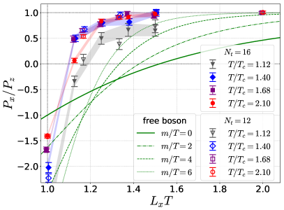
Figure 3: Ratio $P_{x}/P_{z}$ as a function of $L_{x}T$ for various values of $T/T_{c}$. Error bars include statistical error and systematic ones from (1) the choice of the fit range and (2) $\pm 3\%$ uncertainty of $\Lambda_{\overline{\mathrm{MS}}}$; see the text. The behavior of $P_{x}/P_{z}$ in the free scalar theory is also shown by the lines for several values of mass temperature ratio $m/T$. Shaded bands connect error bars at $N_{\tau}=16$. The data points at $T/T_{c}=1.40$ (1.68) are shifted toward right (left) slightly.

Now, let us first focus on the ratio $P_{x}/P_{z}$. In Fig. 3, we show the $t\to 0$ extrapolated results of $P_{x}/P_{z}$ as a function of $L_{x}T$ at four temperatures, $T/T_{c}=1.12$, $1.40$, $1.68$, and $2.10$. The results for $N_{\tau}=16$ and $12$ are shown by the filled and open symbols, respectively. Error bars include systematic error from the choice of the fitting range and the uncertainty of $\Lambda_{\overline{\mathrm{MS}}}$ estimated from $\pm 3\%$ variation, as well as the statistical one. The comparison of the results for $N_{\tau}=16$ and $12$ shows that a significant lattice spacing dependence is not observed, as anticipated from the discussion in Sec. V.1.

In Fig. 3, we also show the ratio $P_{x}/P_{z}$ obtained in the free scalar theory with mass $m$ for several values of $m/T$. The result for $m=0$ is taken from Ref. Mogliacci et al. (2018), while the procedure to obtain the results at $m\neq 0$ will be reported in a future publication Mogliacci et al. .

As discussed in Sec. II, $P_{x}/P_{z}$ approaches unity in the $L_{x}T\to\infty$ limit. In the free massless theory, a clear deviation of $P_{x}/P_{z}$ from this limiting value is already observed at $L_{x}T=2$, and the ratio crosses zero at $L_{x}T\simeq 1.5$. At $L_{x}T=1$, the ratio is $P_{x}/P_{z}=-1$, as suggested from Eq. (5) and the fact that $\Delta=0$ in this theory.

The results of SU(3) YM theory shown in Fig. 3 behave quite differently from the massless free theory. In SU(3) YM theory, $P_{x}/P_{z}=1$ within statistics at $L_{x}T=1.5$ for $1.4\leq T/T_{c}\leq 2.1$. Even at $L_{x}T=1.333$ and $1.375$, deviation from $P_{x}/P_{z}=1$ is comparable with the error for these temperatures. By decreasing $L_{x}T$ further, the ratio suddenly becomes smaller and arrives at $P_{x}/P_{z}<-1$ at $L_{x}T=1$. It is interesting to note that almost the same $L_{x}T$ dependence is observed for $1.4\leq T/T_{c}\leq 2.1$, while the result near $T_{c}$ at $T/T_{c}=1.12$ shows a deviation from this trend. From these results, it is concluded that the SU(3) YM theory at $1.4\leq T/T_{c}\leq 2.1$ is remarkably insensitive to the PBC with length $L_{x}$ compared with the massless free theory. At $T/T_{c}=1.12$, the SU(3) YM theory is however clearly more sensitive to the PBC. This may be important for future phenomenological applications.

In the free scalar theory, $P_{x}/P_{z}$ approaches unity as $m/T$ becomes larger for large $L_{x}T$ as shown in Fig. 3. Therefore, the lattice results might be partially understood as the effect of nonzero $m$. However, even at $m/T=6$ the behavior is still inconsistent with the lattice result. Also, $P_{x}/P_{z}$ at $L_{x}T=1$ becomes smaller as $m/T$ becomes larger, which is inconsistent with the lattice result.

Figure 4: Dependences of $P_{x}/T^{4}$ (upper-left), $P_{z}/T^{4}$ (upper-right), $\varepsilon/T^{4}$ (lower-left), and $\Delta/T^{4}$ (lower-right) on $L_{x}T$ for several values of $T/T_{c}$. Dashed vertical lines in the upper (middle and lower) panel(s) show the value of $\varepsilon/T^{4}$ ($P/T^{4}$) in the isotropic case obtained in Ref. Iritani et al. (2019), with the error shown by the shaded region.

Shown in Fig. 4 are the behavior the longitudinal and transverse pressures $P_{x}$ and $P_{z}$, the energy density $\varepsilon$, and $\Delta$ as functions of $L_{x}T$. For guides of these results, we also show the continuum extrapolated values of $P/T^{4}$, $\varepsilon/T^{4}$, and $(\varepsilon-3P)/T^{4}$ in the isotropic case obtained in Ref. Iritani et al. (2019) by the horizontal dashed lines for $T/T_{c}=1.12,~{}1.40,~{}1.68$, with the errors shown by the shaded region. From Fig. 4, one finds that these quantities are insensitive to the existence of the boundary for $L_{x}T\gtrsim 1.3$ for $T/T_{c}=1.40,~{}1.68,~{}2.10$.

V.4 High temperature

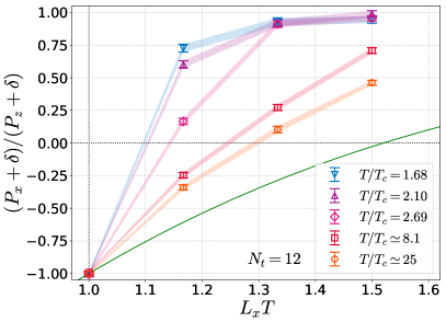
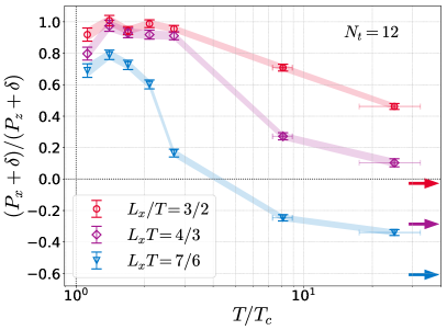
Figure 5: Ratio $(P_{x}+\delta)/(P_{z}+\delta)$ for various values of $T$ and $L_{x}T$. Upper (Lower) panel shows the ratio as a function of $L_{x}T$ ($T/T_{c}$). The solid line in the upper panel shows the ratio in the massless free scalar theory. The arrows at the right in the lower panel shows the ratio in the massless free scalar theory for each $L_{x}T$.

At asymptotically high temperature, the SU(3) YM theory approaches a free gas composed of massless gluons. In this limit, the $L_{x}T$ dependence of $P_{x}/P_{z}$ should approach the massless free scalar theory. It is an interesting question how the results in Fig. 3 approach this asymptotic behavior. The extension of the numerical analysis to high $T$, however, has two difficulties. First, as the lattice spacing $a=(N_{\tau}T)^{-1}$ becomes smaller the lattice size required for the vacuum subtraction becomes huge. Second, the relation between $\beta=6/g_{0}^{2}$ and $a$ is not available for such fine lattice spacings.

Here, to extend our analyses to high temperatures avoiding these difficulties we focus on the ratio

$$\frac{P_{x}+\delta}{P_{z}+\delta},$$ (18)

with $\delta=\Delta/4$. This ratio does not depend on the second term in Eq. (13) proportional to $c_{2}(t)$. One thus can obtain the ratio without the vacuum subtraction. Furthermore, as $c_{1}(t)$ cancels between numerator and denominator in Eq. (18), this ratio is obtained without using $c_{1}(t)$. This means that the lattice spacing in physical units required for the determination of the running coupling in $c_{1}(t)$ Iritani et al. (2019) is not needed to obtain Eq. (18).

In Fig. 5, we show the behavior of Eq. (18) as functions of $L_{x}T$ and $T/T_{c}$ in the upper and lower panels, respectively. The results at $T/T_{c}\simeq 8.1$ and $25$ corresponds to those obtained at $\beta=8.0$ and $9.0$, respectively; see Table 1. Temperatures are deduced from the relation between $\beta$ and $a$ in Ref. Kitazawa et al. (2016), which is reliable for $6.3\leq\beta\leq 7.4$. As $\beta=8.0$ and $9.0$ are outside of this range, the values $T/T_{c}$ should be regarded just as a guide for the true value of $T/T_{c}$. To depict this uncertainty, in the lower panel we show $10\%$ and $30\%$ error bars in $T/T_{c}$ for the data points at $\beta=8.0$ and $9.0$.

In the upper panel of Fig. 5, we show the ratio Eq. (18) in the massless free scalar theory by the solid line, while in the lower panel the ratio for each $L_{x}T$ is shown by arrows at right in the panel; note that in the massless theory $\delta=0$. The comparison of the lattice data with these results shows that the former approaches the asymptotic value as $T$ is increased, but the difference is still large even at the highest temperature $T/T_{c}\simeq 25$.

VI Discussion and Outlook

In the present study, we investigated the energy momentum tensor in 3+1 dimensional SU(3) YM theory at $T>T_{c}$ in anisotropic finite volume systems with the PBC. We chose to make one direction small, $L_{x}T\sim 1$, while keeping the other two spatial dimensions large, $L_{y,z}T\gg 1$. We found that, as shown in Fig. 3, a clear anisotropy in the stress tensor is observed only for $L_{x}T\lesssim 1.3$ for $1.4\leq T/T_{c}\leq 2.1$. In free scalar theory with the same boundary condition, a significant anisotropy manifests itself at much larger values of $L_{x}T$. One therefore concludes that SU(3) YM theory near but above $T_{c}$ is remarkably insensitive to the existence of the periodic boundary. Even allowing the free scalar particles to have a mass $m=6T$ was insufficient to reproduce the insensitivity to the presence of the finite periodic boundary in SU(3) YM theory.

At the scales probed by these temperatures the running coupling is $g(2\pi T)\sim 2$, and the leading order, infinite volume thermal field theory result for the Debye mass of the gluon is $m_{D}\sim gT$. That the effective free quasiparticle mass required to mimic the results of the full SU(3) YM theory is so large indicates that 1) finite-size corrections to the infinite and isotropic volume leading order thermal field theory result are large, for example the Debye gluon mass — which by dimensional analysis is given by $m_{D}/g=f_{T}(L_{x}T)T+f_{L_{x}}(L_{x}T)/L_{x}$ — might pick up large finite-size corrections, 2) the interactions of the full theory cannot be easily approximated by a free quasiparticle theory, or 3) that there are important non-perturbative dynamics at these scales.

Investigating 1) is an important avenue for future analytic research, especially as the work here possibly suggests that the finite-size corrections to the effective gluon mass are large. 2) is quite likely given than other thermodynamic properties computed from the lattice at these temperature scales are only well approximated by resummed thermal field theory at three or four loops Andersen et al. (2013); Mogliacci et al. (2013); Haque et al. (2014). 3) must also contribute: Forty years ago, Linde demonstrated Linde (1980) the possibility for an infrared cutoff of order ${\cal O}\left(g^{2}T\right)$ to appear in the thermodynamics of a YM gas in an isotropic infinite volume. This effectively led to the findings of a non-perturbative coefficient in the pressure, when probed perturbatively Di Renzo et al. (2006). More recently, the presence of the very same type of (Linde) problem was discovered in an anisotropic volume of SU(3) YM theory Fraga et al. (2017), such as the one we use here. These works obviously raise the need for a better understanding of the possible presence of a non-perturbative scale such as $\sim g\sqrt{T/L_{x}}$ in the thermodynamics of anisotropic volumes of the SU(3) YM theory. It is then an interesting future work to pursue the physical origin from the knowledge of the Casimir effect in various theories and settings Meyer (2009); Karabali and Nair (2018); Chernodub et al. (2018); Ishikawa et al. (2019); Chernodub et al. (2019).

The remarkably large effective quasiparticle mass required to mimic the lattice results suggests a larger-than-expected effective Debye mass for gluons at temperatures on the order of $T_{c}$. A larger Debye mass implies a stronger-than-expected screening of color charges in the thermal medium, which would lead to a smaller-than-expected coupling of high momentum particles to the small system plasma medium. This reduction in coupling would naturally lead to a smaller-than-expected energy loss for these high momentum particles compared to propagation in larger systems at the same temperature. This reduction in energy loss would provide a natural explanation for the current lack of evidence for high momentum particle suppression in small systems Kolbe and Horowitz (2015).

The finite-size effects investigated in the present study are likely to have implications in the phenomenological studies of relativistic heavy-ion collisions Song et al. (2011); Gale et al. (2013); Weller and Romatschke (2017). A direct implication of our work is concerned with the finite-volume effect in the hot medium created by the heavy-ion collisions. Our results suggest that the effects of such anisotropic finite volumes would not strongly affect the thermodynamics of the medium, provided that our results obtained with the PBC are directly applicable to heavy-ion physics. The medium created in heavy-ion collisions indeed has a finite-volume and a strong anisotropic geometry. It would also be an interesting subject to pursue the connection of our study with systems having strong pressure anisotropy, such as the initial stage of the collisions.

Although we constrained our attention to a system with PBC for one direction in the present study, it is a straightforward extension of this study to perform similar analyses with other boundary conditions (see Ref. Mogliacci et al. (2018) for more details on the possible relevance of different boundary conditions). For example, it is also possible to impose anti-periodic or Dirichlet boundary conditions, instead of the PBC. Furthermore, it is possible to impose boundary conditions for two or all the directions Mogliacci et al. (2018). Among them, the simulation with the anti-periodic boundary conditions seems especially interesting, because the numerical analysis with this conditions can be carried out straightforwardly, and this boundary condition eliminates the zero mode contribution (in fact, much like the Dirichlet condition Mogliacci et al. (2018)) which is the origin of the infrared divergences plaguing all theories with massless bosonic fields.

Finally, although in the present study we focused on the pressure anisotropy induced by the periodic boundary conditions in the SU(3) YM theory at finite temperature, our numerical analysis can be used for more general systems having anisotropy such as full QCD with strong magnetic field Buividovich et al. (2010); D’Elia et al. (2010); Bali et al. (2012); Bruckmann et al. (2013).