Correlations of Energy-Momentum Tensor via Gradient Flow
in SU(3) Yang-Mills Theory at Finite Temperature

Abstract

Euclidean two-point correlators of the energy-momentum tensor (EMT) in SU(3) gauge theory on the lattice are studied on the basis of the Yang-Mills gradient flow. The entropy density and the specific heat obtained from the two-point correlators are shown to be in good agreement with those from the one-point functions of EMT. These results constitute a first step toward the first principle simulations of the transport coefficients with the gradient flow.

Various thermal and transport properties of quantum field theories are encoded in the correlations of energy-momentum tensor (EMT) at finite temperature ($T$). In particular, fluctuation and transport properties of hot QCD (Quantum ChromoDynamics) matter at finite $T$ have attracted a lot of attention in relation to the phenomenological studies on relativistic heavy-ion collisions Hirano:2012kj ; Asakawa:2015ybt .

Although the non-perturbative investigations of the EMT at finite $T$ using lattice QCD simulations have been very difficult owing to the lack of translational and rotational symmetry Caracciolo:1990emt ; Suzuki:2016ytc , a novel method to construct the EMT on the lattice Suzuki:2013gza on the basis of the gradient flow Narayanan:2006rf ; Luscher:2010iy ; Luscher:2011bx was recently proposed and was successfully applied to the equation of states in pure gauge theory Asakawa:2013laa ; Kamata:2016any ; Kitazawa:2016dsl . This study shows that the thermodynamical observables such as the energy density and pressure extracted from the expectation values of the EMT (the one-point functions) agree extremely well with previous high-precision results using the integral method Boyd:1996bx ; Okamoto:1999hi ; Borsanyi:2012ve . Also, the statistics required in the new method is substantially smaller than that in the previous method. The method is now extended to full QCD simulations at finite $T$ Makino:2014taa ; Taniguchi:2016ofw .

In the present paper, we report our exploratory studies to extend the previous results of the one-point functions to the two-point EMT correlators in SU(3) lattice gauge theory Kitazawa:2014uxa . The advantages of such extension are threefold. First of all, the method allows direct access to the specific heat $c_{V}$ and entropy density $s$ from the EMT correlations. Secondly, one could explicitly check the conservation law of EMT obtained by the gradient flow. Thirdly, the method will open the new door to the study of important transport coefficients such as the shear and bulk viscosities Karsch:1986cq ; Nakamura:2004sy ; Huebner:2008as ; Meyer:2011gj ; Astrakhantsev:2017nrs . We will focus on the first two aspects in this paper.

Let us here summarize the properties of the correlators of the EMT, ${\cal T}_{\mu\nu}(x)$, in the Euclidean and continuum spacetime, where $x_{\mu=1,2,3,4}=(\vec{x},\tau)$ with $0\leq\tau<1/T$. We define a dimensionless temporal correlator of ${\cal T}_{\mu\nu}(x)$ at finite $T$ and at finite volume $V$ as

$$C_{\mu\nu;\rho\sigma}(\tau)\equiv\frac{1}{T^{5}}\int_{V}d^{3}x\langle\delta{\cal T}_{\mu\nu}(x)\delta{\cal T}_{\rho\sigma}(0)\rangle,$$ (1)

where $\langle\cdot\rangle$ denotes the thermal average. We have defined $\delta{\cal T}_{\mu\nu}(x)\equiv{\cal T}_{\mu\nu}(x)-\langle{\cal T}_{\mu\nu}(x)\rangle$, so that $C_{\mu\nu;\rho\sigma}(\tau)$ contains only connected contribution. Owing to the conservation of the EMT in the Euclidean space-time ($\partial_{\mu}{\cal T}_{\mu\nu}=0$), we have $\frac{d}{d\tau}\overline{\cal T}_{4\nu}=0$ with $\overline{\cal T}_{\mu\nu}\equiv\int_{V}d^{3}x\ {\cal T}_{\mu\nu}(x)$. For $\tau\neq 0$, this leads to

$$\frac{d}{d\tau}C_{4\nu;\rho\sigma}(\tau)=0.$$ (2)

Since the energy density of the system is represented as $\varepsilon=-\langle\overline{\cal T}_{44}\rangle/V$, the specific heat per unit volume $c_{V}$ is given by Asakawa:2015ybt

$$\frac{c_{V}}{T^{3}}=\frac{1}{T^{3}}\frac{d\varepsilon}{dT}=\frac{\langle(\delta\overline{\cal T}_{44})^{2}\rangle}{VT^{5}}=C_{44;44}(\tau),$$ (3)

where Eq. (2) is used in the last equality. Note that $\tau$ can be taken anywhere in the range $0<\tau<1/T$ owing to the EMT conservation.

Similarly, from the thermodynamic relation for entropy density $s=dp/dT=(1/V)d\langle\overline{\cal T}_{11}\rangle/dT$ Landau-Lifshitz , one obtains

$$\frac{s}{T^{3}} =\frac{1}{T^{3}}\frac{dp}{dT}=\frac{\langle\delta\overline{\cal T}_{44}\delta\overline{\cal T}_{11}\rangle}{VT^{5}}=-C_{44;11}(\tau).$$ (4)

Again, $\tau$ can be taken arbitrarily in $0<\tau<1/T$.

Finally, the momentum fluctuation is related to the enthalpy density $h$ Giusti:2010bb ; Minami:2012hs ,

$$\frac{h}{T^{4}}=\frac{\langle(\delta\overline{T}_{41})^{2}\rangle}{VT^{5}}=-C_{41;41}(\tau).$$ (5)

At zero chemical potential, $h=\varepsilon+p=sT$.

In the present study, we use the EMT operator defined through the gradient flow Suzuki:2013gza . The gradient flow for Yang-Mills gauge field is defined by the differential equation with respect to the hypothetical 5-th coordinate $t$ Luscher:2010iy

$$\frac{dA_{\mu}(t,x)}{dt}=-g_{0}^{2}\frac{\delta S_{\rm YM}(t)}{\delta A_{\mu}(t,x)}=D_{\nu}G_{\nu\mu}(t,x),$$ (6)

with the Yang-Mills action $S_{\rm YM}(t)$ and the field strength $G_{\mu\nu}(t,x)$ composed of the transformed field $A_{\mu}(t,x)$. The flow time $t$ has a dimension of inverse mass squared. The initial condition at $t=0$ is taken for the field in the conventional gauge theory; $A_{\mu}(0,x)=A_{\mu}(x)$. The gradient flow for positive $t$ acts as the smearing of the gauge field with the smearing radius $\sqrt{8t}$  Luscher:2010iy . The EMT operator is then defined as

$${\cal T}_{\mu\nu}(x) = \lim_{t\to 0}{\cal T}_{\mu\nu}(t,x),$$ (7)

$${\cal T}_{\mu\nu}(t,x) = \frac{U_{\mu\nu}(t,x)}{\alpha_{U}(t)}+\frac{\delta_{\mu\nu}}{4\alpha_{E}(t)}\left[E(t,x)-\left\langle E(t,x)\right\rangle_{0}\right],$$

where the dimension-four gauge-invariant operators on the right hand side are given by Suzuki:2013gza

$$E(t,x) =\frac{1}{4}G_{\mu\nu}^{a}(t,x)G_{\mu\nu}^{a}(t,x),$$ (9)

$$U_{\mu\nu}(t,x) =G_{\mu\rho}^{a}(t,x)G_{\nu\rho}^{a}(t,x)-\delta_{\mu\nu}E(t,x),$$ (10)

while $\langle E(t,x)\rangle_{0}$ in Eq. (LABEL:eq:T) is the vacuum expectation value of $E(t,x)$, which is introduced so that $\langle{\cal T}_{\mu\nu}(x)\rangle$ vanishes in the vacuum. The coefficients $\alpha_{U}(t)$ and $\alpha_{E}(t)$ have been calculated perturbatively in Ref. Suzuki:2013gza for small $t$: Their explicit forms in the $\overline{\mathrm{MS}}$ scheme are given in Ref. Kitazawa:2016dsl .

Although Eqs. (7) and (LABEL:eq:T) are exact in the continuum spacetime, special care is required in lattice gauge theory with finite lattice spacing $a$: The flow time should satisfy $\sqrt{8t}\gtrsim a$ to suppress the lattice discretization effects. It has been shown for the thermal average of the EMT that there exists indeed a range of $t$ for sufficiently small $a$, so that the lattice data allow reliable extrapolation to $t=0$ to obtain $\varepsilon$ and $p$ Asakawa:2013laa ; Kamata:2016any ; Kitazawa:2016dsl .

To analyze the two-point EMT correlations with Eq. (LABEL:eq:T), we have an extra condition that the distance between the two smeared operators $\tau$ in temporal direction is well separated (with the temporal periodicity) to avoid their overlap. Because the smearing length along temporal direction is $\sqrt{2t}$, the necessary conditions read $a\lesssim 2\sqrt{2t}\lesssim\tau\leq 1/(2T)$, or equivalently, in terms of the dimensionless quantities, as

$$\frac{1}{N_{\tau}}\lesssim\sqrt{8tT^{2}}\lesssim\tau T\leq\frac{1}{2}$$ (11)

with $N_{\tau}=(aT)^{-1}$ being the temporal lattice size.

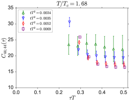
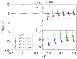
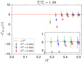
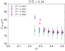
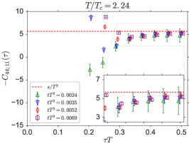
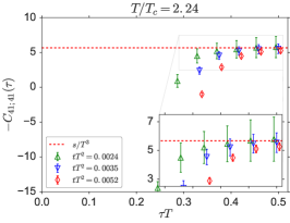
Figure 1: Correlators $C_{44;44}(\tau)$ (left), $C_{44;11}(\tau)$ (middle), and $C_{41,41}(\tau)$ (right) for several values of flow time $t$ for $N_{\tau}=24$. The red dashed lines show $s/T^{3}=(\varepsilon+p)/T^{4}$ obtained from the one-point function of the EMT with the same gauge configurations.

$T/T_{\rm c}=1.68$
$N_{s}$	$N_{\tau}$	$\beta$	$N_{\rm conf}$
96	24	7.265	200,000
64	16	6.941	180,000
48	12	6.719	180,000

$T/T_{\rm c}=2.24$
$N_{s}$	$N_{\tau}$	$\beta$	$N_{\rm conf}$
96	24	7.500	200,000
64	16	7.170	180,000
48	12	6.943	180,000

Table 1: Simulation parameters on the lattice: $N_{s}$, $N_{\tau}$, $\beta=6/g_{0}^{2}$, and $N_{\rm conf}$ are spatial lattice size, temporal lattice size, the bare coupling constant, and the total number of gauge configurations, respectively.

In our numerical studies, we consider SU(3) Yang-Mills theory on four-dimensional Euclidean lattice and employ the Wilson gauge action under the periodic boundary condition. Gauge configurations are generated by the same procedure as in Ref. Kitazawa:2016dsl , but each measurement is separated by $50$ sweeps. Statistical errors are estimated by the jackknife method with $100$ jackknife samples. On the right hand side of the flow equation Eq. (6), the Wilson gauge action is used for $S_{\rm YM}(t)$, while the operators in Eqs. (9) and (10) are constructed from $G^{a}_{\mu\nu}(t,x)$ defined by the clover-type representation.

We study two cases above the deconfinement transition, $T/T_{\rm c}=1.68$ and $2.24$, with three different lattice volumes $N_{s}^{3}\times N_{\tau}$ with a fixed aspect ratio $N_{s}/N_{\tau}=4$. The values of $\beta=6/g_{0}^{2}$ corresponding to each set of $T/T_{\rm c}$ and $N_{\tau}$ are obtained from Refs. Asakawa:2015vta ; Kitazawa:2016dsl . The resultant simulation parameters are summarized in Table 1.

Shown in Fig. 1 are the $\tau$ dependences of $C_{44;44}(\tau)$, $C_{44;11}(\tau)$, and $C_{41;41}(\tau)$ for $T/T_{\rm c}=1.68$ (upper panels) and $T/T_{\rm c}=2.24$ (lower panels) for $N_{\tau}=24$ with typical values of $tT^{2}$ between the upper and lower bounds in Eq. (11). From the overall behavior of the lattice data in these figures, one finds two key features: (i) As $t$ decreases, the data start to show the plateau structure for $\tau T\gtrsim 0.3$. (ii) As $t$ decreases, the statistical errors become larger. The feature (i) is a signature of the EMT conservation Eq. (2) for large $\tau$, where the smeared EMT operators do not overlap with each other. The feature (ii) is due to the fact that the gauge fields are rough (smooth) for small (large) $t$.

Shown by the red dashed lines in Fig. 1 together with $C_{44;11}(\tau)$ and $C_{41;41}(\tau)$ are $s/T^{3}=(\varepsilon+p)/T^{4}$ obtained by the one-point function of EMT ($\langle\overline{\cal T}_{44}\rangle$ and $\langle\overline{\cal T}_{11}\rangle$) using the method in Ref. Kitazawa:2016dsl with the same configurations. This agreement of the results of $s/T^{3}$ between the one-point function and the two-point functions, as it should be for Eqs. (4) and (5), at large $\tau$ and small $t$ indicates an internal consistency of the present method.

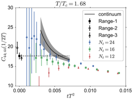
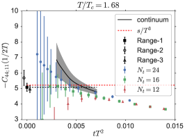
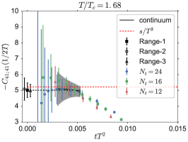
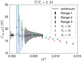
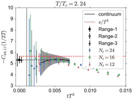
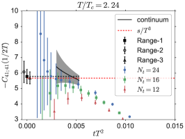
Figure 2: $t$ dependences of the midpoint correlators $C_{44,44}(\tau_{m})$ (left), $C_{44,11}(\tau_{m})$ (middle), and $C_{41,41}(\tau_{m})$ (right) for $T/T_{\rm c}=1.68$ and $2.24$. The black lines show the results of continuum extrapolation using $N_{\tau}=12,16$, and $24$.

To take the continuum limit $a\rightarrow 0$ followed by an extrapolation $t\rightarrow 0$, we show, in Fig. 2, the $t$ dependence of the correlators for different lattice spacings, $a=1/(N_{\tau}T)$. Here we choose the maximum possible separation, $\tau=\tau_{m}=1/(2T)$, to minimize the overlap of the EMT operators. The continuum extrapolation is carried out by using the data at $N_{\tau}=12$, $16$, and $24$ for each $t\in[t_{\rm min},t_{\rm max}]$ with an ansatz $C_{\mu\nu;\rho\sigma}(\tau_{m})|_{{}_{\rm lat}}=C_{\mu\nu;\rho\sigma}(\tau_{m})|_{{}_{\rm cont}}+O(a^{2})$ expected from perturbation theory. Here $t_{\rm min,~{}max}$ is chosen in such a way that $C_{4\nu;\rho\sigma}(\tau_{m})/C_{4\nu;\rho\sigma}(\tau_{m}-a)=1$ within the statistical errors: This procedure excludes the small $t$ region where large lattice discretization errors arise, as well as the large $t$ region where the systematic errors from the overlap of EMT operators and the contribution of higher dimensional operators other than Eqs. (9) and (10) are not negligible Kitazawa:2016dsl . The resulting ranges in the dimensionless combination are $(tT^{2})_{\rm min}=0.003$ and $(tT^{2})_{\rm\max}=0.007$ for $C_{44;44}(\tau_{m})$, and $(tT^{2})_{\rm min}=0.003$ and $(tT^{2})_{\rm max}=0.006$ for $C_{44;11}(\tau_{m})$ and $C_{41;41}(\tau_{m})$.

The results of the continuum extrapolation are shown by the black lines with the error represented by the gray band in Fig. 2. At the level of error bars in the present exploratory study, we do not have enough resolution to reliably extract the $O(t)$ contribution in $C_{\mu\nu;\rho\sigma}(\tau_{m})$ Kitazawa:2016dsl , so that we take the $t\to 0$ extrapolation by a constant fit in the interval $[t_{\rm min},t_{\rm max}]$, which is called Range-1. The final results after the double extrapolation ($t\to 0$ after $a\to 0$) are shown by the filled squares in Fig. 2. To estimate the systematic errors from this constant fit, we choose the Range-2 (the first half of Range-1) and Range-3 (the latter half of Range-1); the results are shown by open circles and open triangles, respectively. The red dashed lines in the middle and right panels in Fig. 2 are $s/T^{3}$ obtained from the one-point function of EMT.

$s/T^{3}$
$T/T_{\rm c}$	$C_{44;11}(\tau_{m})$	$C_{41;41}(\tau_{m})$	$\langle{\cal T}_{\mu\nu}\rangle$	ideal gas
1.68	5.08(26)$(^{+60}_{-11}$)	5.02(47)$(^{+7}_{-2})$	5.222(10)(24)	7.02
2.24	5.34(28)$(^{+0}_{-0}$)	5.78(46) $(^{+29}_{-10})$	5.675(10)(24)	7.02

Table 2: Values of $s/T^{3}$ obtained from Eqs. (4) and (5) together with those obtained from the one-point function of EMT. The ideal gas limit for massless gluons is also shown for comparison. The first (second) parenthesis shows statistical (systematic) error. The systematic error for the one-point function originates from the 1% uncertainty of $\Lambda_{\overline{\rm MS}}$ Kitazawa:2016dsl .

$c_{V}/T^{3}$
$T/T_{\rm c}$	$C_{44;44}(\tau_{m})$	Ref. Gavai:2004se	Ref. Borsanyi:2012ve	ideal gas
1.68	17.7(8)$(^{+2.1}_{-0.4})$	22.8(7)∗	17.7	21.06
2.24	17.5(8)$(^{+0}_{-0.1})$	17.9(7)∗∗	18.2	21.06

Table 3: Values of $c_{V}/T^{3}$ obtained by Eq. (3) as well as those obtained directly from the differential method Gavai:2004se and those calculated indirectly from $\varepsilon(T)$ in the integral method Borsanyi:2012ve . The ideal gas limit for massless gluons is also shown for comparison. The error bars are estimated in the same way as $s/T^{4}$ in Table 2. The symbol $*$ ($**$) indicates that the numbers are for $T/T_{c}=1.5~{}(2.0)$. The error bars of $c_{V}/T^{3}$ in the column Ref. Borsanyi:2012ve would be a few % level.

Shown in Table 2 are the numerical results of $s/T^{3}$ obtained in the present analysis of EMT correlators. Within the statistical and systematic error bars, the results of the two different correlators agree with each other, and they agree to the results of the one-point function of EMT. Also the central value of $s/T^{3}$ in our analysis increases as $T$ and also much less than the ideal gas value, which captures the essential feature expected from strongly interacting gluon plasma above $T_{\rm c}$.

Shown in Table 3 are the numerical results of $c_{V}/T^{3}$ obtained in the present analysis of EMT correlators. Our results agree quantitatively with the numbers extracted from the recent high-precision study of the energy density in the integral method Borsanyi:2012ve and qualitatively with the numbers obtained in the differential method Gavai:2004se . Our specific heat is about 20% smaller than the ideal gas value, which also indicates the strong coupling feature of the system.

In summary, we have investigated the two-point EMT correlators in SU(3) Yang-Mills theory at finite temperature ($T/T_{\rm c}=2.24$ and $1.68$) using the method of gradient flow with the flow time $t$. The correlators $C_{4\nu;\rho\sigma}(\tau)$ approach constant values for sufficiently large $\tau$ and small $t$. This is an indication that the conservation of the EMT is realized in the gradient flow as long as the two EMT operators do not have overlap with each other. By taking the double limit ($t\rightarrow 0$ after $a\rightarrow 0$) using the data for $N_{\tau}=12$, $16$, and $24$, we found that the entropy density ($s$) obtained from the two-point EMT correlators ($C_{44;11}(\tau_{m})$ and $C_{41;41}(\tau_{m})$) reproduces the high precision result previously obtained from the one-point function. Also, we found that the specific heat ($c_{V}$) can be determined in 5-10% accuracy from the two-point EMT correlator ($C_{44;44}(\tau_{m})$) even with relatively low statistics. Now that we have confirmed that thermodynamical quantities are obtained accurately with two-point EMT correlators with the gradient flow, it is within reach to investigate transport coefficients with two-point EMT correlations as well.

Although we focused on SU(3) Yang-Mills theory in this study, the same analysis can be also performed in full QCD Makino:2014taa ; Taniguchi:2016ofw . A preliminary study along this line is reported in Ref. Taniguchi:2017 .

The authors thank E. Itou and H. Suzuki for discussions in the early stage. Numerical simulation was carried out on IBM System Blue Gene Solution at KEK under its Large-Scale Simulation Program (Nos. 13/14-20, 14/15-08, 15/16-15, 16/17-07). This work was supported by JSPS KAKENHI Grant Numbers JP17K05442 and 25287066. TH were partially supported by the RIKEN iTHES Project and iTHEMS Program. TH is grateful to the Aspen Center for Physics, supported by NSF Grant PHY1607611, where part of this research was done.

References

- (1) T. Hirano, P. Huovinen, K. Murase, and Y. Nara, Prog. Part. Nucl. Phys. 70, 108 (2013) [arXiv:1204.5814 [nucl-th]].
- (2) M. Asakawa and M. Kitazawa, Prog. Part. Nucl. Phys. 90, 299 (2016) [arXiv:1512.05038 [nucl-th]].
- (3) S. Caracciolo, G. Curci, P. Menotti, and A. Pelissetto, Annals Phys. 197, 119 (1990).
- (4) H. Suzuki, PoS LATTICE 2016, 002 (2017) [arXiv:1612.00210 [hep-lat]], and references therein.
- (5) H. Suzuki, PTEP 2013, no. 8, 083B03 (2013) [Erratum: PTEP 2015, no. 7, 079201 (2015)] [arXiv:1304.0533 [hep-lat]].
- (6) R. Narayanan and H. Neuberger, JHEP 0603, 064 (2006) [hep-th/0601210].
- (7) M. Lüscher, JHEP 1008, 071 (2010) [arXiv:1006.4518 [hep-lat]].
- (8) M. Lüscher and P. Weisz, JHEP 1102, 051 (2011) [arXiv:1101.0963 [hep-th]].
- (9) M. Asakawa et al. [FlowQCD Collaboration], Phys. Rev. D 90, no. 1, 011501 (2014) Erratum: [Phys. Rev. D 92, no. 5, 059902 (2015)] [arXiv:1312.7492 [hep-lat]].
- (10) N. Kamata and S. Sasaki, Phys. Rev. D 95, no. 5, 054501 (2017) [arXiv:1609.07115 [hep-lat]].
- (11) M. Kitazawa, T. Iritani, M. Asakawa, T. Hatsuda, and H. Suzuki, Phys. Rev. D 94, no. 11, 114512 (2016) [arXiv:1610.07810 [hep-lat]].
- (12) L. Giusti and H. B. Meyer, Phys. Rev. Lett. 106, 131601 (2011) [arXiv:1011.2727 [hep-lat]]; JHEP 1301, 140 (2013) [arXiv:1211.6669 [hep-lat]].
- (13) L. Giusti and M. Pepe, Phys. Rev. D 91, 114504 (2015) [arXiv:1503.07042 [hep-lat]].
- (14) G. Boyd, J. Engels, F. Karsch, E. Laermann, C. Legeland, M. Lutgemeier, and B. Petersson, Nucl. Phys. B 469, 419 (1996) [hep-lat/9602007].
- (15) M. Okamoto et al. [CP-PACS Collaboration], Phys. Rev. D 60, 094510 (1999) [hep-lat/9905005].
- (16) S. Borsanyi, G. Endrodi, Z. Fodor, S. D. Katz, and K. K. Szabo, JHEP 1207, 056 (2012) [arXiv:1204.6184 [hep-lat]].
- (17) H. Makino and H. Suzuki, PTEP 2014, no. 6, 063B02 (2014) [Erratum: PTEP 2015, no. 7, 079202 (2015)] [arXiv:1403.4772 [hep-lat]].
- (18) Y. Taniguchi, S. Ejiri, R. Iwami, K. Kanaya, M. Kitazawa, H. Suzuki, T. Umeda, and N. Wakabayashi, arXiv:1609.01417 [hep-lat].
- (19) Preliminary results of this study is reported in M. Kitazawa, et al. PoS LATTICE 2014, 022 (2014) [arXiv:1412.4508 [hep-lat]].
- (20) F. Karsch and H. W. Wyld, Phys. Rev. D 35, 2518 (1987).
- (21) A. Nakamura and S. Sakai, Phys. Rev. Lett. 94, 072305 (2005) [hep-lat/0406009].
- (22) K. Huebner, F. Karsch, and C. Pica, Phys. Rev. D 78, 094501 (2008) [arXiv:0808.1127 [hep-lat]].
- (23) H. B. Meyer, Eur. Phys. J. A 47, 86 (2011) [arXiv:1104.3708 [hep-lat]].
- (24) N. Astrakhantsev, V. Braguta, and A. Kotov, JHEP 1704, 101 (2017) [arXiv:1701.02266 [hep-lat]].
- (25) L.D. Landau and E.M. Lifshitz, “Statistical Physics, Part 1” (3rd edition), (Pergamon Press, Oxford, NY (1980)).
- (26) Y. Minami and Y. Hidaka, Phys. Rev. E 87, no. 2, 023007 (2013) [arXiv:1210.1313 [hep-ph]].
- (27) M. Asakawa, T. Hatsuda, T. Iritani, E. Itou, M. Kitazawa, and H. Suzuki, arXiv:1503.06516 [hep-lat].
- (28) R. V. Gavai, S. Gupta, and S. Mukherjee, Phys. Rev. D 71 (2005) 074013 [hep-lat/0412036]; Pramana 71, 487 (2008) [hep-lat/0506015].
- (29) Y. Taniguchi, Talk given at Lattice 2017, Granada, Spain, 18-24 June, 2017.