Integral Reduction with Kira 2.0 and
Finite Field Methods

Abstract

We present the new version 2.0 of the Feynman integral reduction program Kira and describe the new features. The primary new feature is the reconstruction of the final coefficients in integration-by-parts reductions by means of finite field methods with the help of FireFly. This procedure can be parallelized on computer clusters with MPI. Furthermore, the support for user-provided systems of equations has been significantly improved. This mode provides the flexibility to integrate Kira into projects that employ specialized reduction formulas, direct reduction of amplitudes, or to problems involving linear system of equations not limited to relations among standard Feynman integrals. We show examples from state-of-the-art Feynman integral reduction problems and provide benchmarks of the new features, demonstrating significantly reduced main memory usage and improved performance w.r.t. previous versions of Kira.

Keywords: Feynman diagrams, multi-loop Feynman integrals, dimensional regularization, Laporta algorithm, modular arithmetic, computer algebra

11em() TTK-20-24
P3H-20-041
FR-PHENO-2020-11
MITP/20-044

NEW VERSION PROGRAM SUMMARY

Program title: Kira

Developer’s repository link: https://gitlab.com/kira-pyred/kira

Licensing provisions: GNU General Public License 3 (GPL)

Programming language: C++

Journal Reference of previous version: P. Maierhöfer, J. Usovitsch and P. Uwer, Kira—A Feynman integral reduction program, Comput. Phys. Commun. 230 (2018) 99 [1705.05610].

Does the new version supersede the previous version?: Yes.

Reasons for the new version: Implementation of new features, some of which improve the performance significantly for many problems.

Summary of revisions: The primary new feature is the reconstruction of the final coefficients in integration-by-parts reductions by means of finite field methods with the help of FireFly [1,2]. This procedure can be parallelized on computer clusters with MPI. Further improvements include the expanded support for user-provided systems of equations as well as a new feature to reduce the main memory usage when generating the system of equations.

Nature of problem: The reduction of Feynman integrals to a smaller set of master integrals is a central strategy for high precision calculations in theoretical particle physics, e.g. for cross sections. Furthermore, the reduction is a key ingredient in many methods to calculate the master integrals themselves.

Solution method: Kira generates a system of equations employing integration-by-parts [3,4] and Lorentz-invariance identities [5] as well as symmetry relations. Linearly dependent equations are removed and master integrals are identified by solving the system over a finite field. The resulting system can be solved with two methods: Since version 1.0, Kira can solve the system algebraically with the help of Fermat [6]. New in this version is the strategy of solving the system many times over finite fields and reconstructing the master integral coefficients with the help of FireFly [1,2]. Both strategies can also be applied to arbitrary homogeneous linear systems of equations.

References:

[1] J. Klappert and F. Lange, Reconstructing rational functions with FireFly, Comput. Phys. Commun. 247 (2020) 106951 [1904.00009].

[2] J. Klappert, S. Y. Klein and F. Lange, Interpolation of dense and sparse rational functions and other improvements in FireFly, Comput. Phys. Commun. 264 (2021) 107968 2004.01463.

[3] F. V. Tkachov, A theorem on analytical calculability of 4-loop renormalization group functions, Phys. Lett. B 100 (1981) 65.

[4] K. G. Chetyrkin and F. V. Tkachov, Integration by parts: The algorithm to calculate $\beta$-functions in 4 loops, Nucl. Phys. B192 (1981) 159.

[5] T. Gehrmann and E. Remiddi, Differential equations for two-loop four-point functions, Nucl. Phys. B580 (2000) 485 [hep-ph/9912329].

[6] R. H. Lewis, Computer Algebra System Fermat, https://home.bway.net/lewis.

Contents

1. 1 Introduction
2. 2 Preliminaries
   1. 2.1 Feynman integral reduction
   2. 2.2 Finite field and interpolation techniques
3. 3 New Features in Kira 2.0
   1. 3.1 Finite field reduction
   2. 3.2 User-defined systems of equations
   3. 3.3 Iterative reduction
   4. 3.4 Master equations
   5. 3.5 Sectors in big-endian binary notation
   6. 3.6 Setting all integrals in a sector to zero
   7. 3.7 Export reduction rules with kira2file
   8. 3.8 Factor out prefactors with FireFly
   9. 3.9 General propagators
   10. 3.10 Add sectors for preferred master integrals
   11. 3.11 Generate a system of equations for later reduction as user-defined system
4. 4 Benchmarks
   1. 4.1 Runtime reduction with bunches and MPI
   2. 4.2 Reducing the memory footprint with iterative reduction
   3. 4.3 Combining algebraic forward elimination with finite field reduction
   4. 4.4 Double-pentagon topology in five-light-parton scattering
5. 5 Installation
   1. 5.1 Obtaining Kira
   2. 5.2 Prerequisites
   3. 5.3 Compiling Kira with the Meson build system
   4. 5.4 Compiling Kira with the Autotools build system
6. 6 Conclusions

1 Introduction

At the Large Hadron Collider, the high energy regime of the Standard Model is probed with ever increasing accuracy. To meet the precision requirements for many scattering processes, it is indispensable to calculate the cross sections for these processes to high accuracy, often at next-to-next-to-leading order, or, in some cases, even higher [1]. The common strategy to deal with the occurring Feynman integrals in such calculations is to first express all integrals in terms of a basis of master integrals. This so-called reduction is furthermore a key ingredient in many methods to calculate the master integrals themselves [2, 3, 4, 5, 6].

In the last few years, new techniques have been explored and applied to integral reduction problems, employing syzygy equations [7, 8, 9, 10, 11, 12], algebraic geometry [13, 14, 15], intersection numbers [16, 17, 18, 19, 20], finite field and interpolation techniques [21, 22, 23, 24, 25, 26], or special integral representations [27, 28, 29, 30]. But unfortunately, there is still no general algorithm known that directly reduces a given set of integrals in a target-oriented manner. Hence, in most cases the Laporta algorithm [31] remains the method of choice. Several public implementations of the algorithm exist [32, 33, 34, 35], and the implementations are continuously improved to be able to handle increasingly complicated reduction problems.

In this article we present the version 2.0 of Kira, a Feynman integral reduction program based on Laporta’s algorithm that was first introduced in Ref. [35]. The most prominent new feature is the application of finite field methods to reconstruct the coefficients appearing in the integral reduction formulas with the help of FireFly [24, 26]. In many cases this leads to reduced main memory usage and, depending on the underlying problem, also to reduced overall runtime. Furthermore, the reduction can be parallelized on computer clusters using MPI [36]. Pre-release versions of Kira 2.0 have already been successfully used in several projects [37, 38, 39].

This article is organized as follows. In section 2 we introduce some definitions used throughout in this article and briefly discuss Feynman integral reduction and finite field methods for the reconstruction of multivariate rational functions. In section 3 we describe the new features of Kira 2.0 and how to use them. Benchmarks of the new features are presented in section 4. Section 5 explains how to obtain, compile, and install Kira. We conclude in section 6.

2 Preliminaries

2.1 Feynman integral reduction

The primary application of Kira is the reduction of Feynman integrals. Here we introduce the notation and conventions used throughout this publication. A general Feynman integral can be parametrized as

$$T(a_{1},\dots,a_{N})=\int\left(\prod\limits_{i=1}^{L}\mathrm{d}^{d}\ell_{i}\right)\frac{1}{P_{1}^{a_{1}}P_{2}^{a_{2}}\cdots P_{N}^{a_{N}}},$$ (1)

where $P_{j}=q_{j}^{2}-m_{j}^{2}$, $j=1,\dots,N$, are the inverse propagators (omitting the Feynman prescription). The momenta $q_{j}$ are linear combinations of the loop momenta $\ell_{i}$, $i=1,\dots,L$ for an $L$-loop integral, and external momenta $p_{k}$, $k=1,\dots,E$ for $E+1$ external legs (or $E=0$ for vacuum integrals), and $m_{j}$ are the propagator masses. The $a_{j}$ are the (integer) propagator powers. The set of inverse propagators must be complete and independent in the sense that every scalar product of momenta can be uniquely expressed as a linear combination of the $P_{j}$, squared masses $m_{j}^{2}$, and external kinematical invariants. The number of propagators is thus $N=\frac{L}{2}(L+2E+1)$ including auxiliary propagators that only appear with $a_{j}\leq 0$.

Integrals of the form (1) for different values of $a_{j}$ are in general not independent. Integration-by-parts (IBP) identities [40, 41] and Lorentz-invariance (LI) identities [42], as well as symmetry relations lead to linear relations between them. These identities can be used to express all integrals through linear combinations of master integrals, which serve as a basis.

Kira employs a variant of the Laporta algorithm [31]: IBP, LI, and symmetry relations are generated for different values for the $a_{j}$, resulting in a linear system of equations. This system of equations is then systematically solved with a Gauss-type elimination algorithm to express integrals which are regarded more complicated in terms of simpler integrals.

To systematically classify integrals, first, integrals are assigned to so-called topologies based on their respective sets of propagators, i.e. their momenta and masses. Multiple topologies are handled by assigning a unique topology ID to each topology. Furthermore, each integral is assigned a sector

$$S=\sum\limits_{j=1}^{N}2^{j-1}\,\theta(a_{j}-\tfrac{1}{2}),$$ (2)

where $\theta(x)$ is the Heaviside step function. A sector $S$ is called subsector of another sector $S^{\prime}$ (with propagators powers $a^{\prime}_{j}$) if $S<S^{\prime}$ and $a_{j}\leq a^{\prime}_{j}$ for all $j=1,\dots,N$. We denote as top-level sectors those sectors which are not subsectors of other sectors that contain Feynman integrals occurring in the reduction problem at hand. As a measure of complexity it is useful to define the number

$$t=\sum_{j=1}^{N}\theta(a_{j}-\tfrac{1}{2}),$$ (3)

of propagators with positive power, the sum $r$ of all positive powers, and the negative sum of all non-positive powers $s$,

$$r=\sum_{j=1}^{N}a_{j}\theta(a_{j}-\tfrac{1}{2}),\qquad s=-\sum_{j=1}^{N}a_{j}\theta(\tfrac{1}{2}-a_{j}).$$ (4)

These values are used as limits in the choice of the sets $a_{j}$ for which the IBP, LI, and symmetry relations are generated. The sets of $a_{j}$ are chosen such that $r\leq r_{\max}$ and $s\leq s_{\max}$, where $r_{\max}$, and $s_{\max}$ are chosen large enough to cover all relevant integrals in the reduction process, but usually no larger.

Symmetry relations either relate integrals within the same sector, or between two different sectors of the same or different topologies. In case of a symmetry between two sectors, each integral can be expressed as a linear combination of integrals in the respective other sector. Hence, master integrals may only appear in that sector which is considered simpler in the chosen ordering of sectors. In case of a relation between two topologies, integrals are always mapped from the topology with higher ID to the one with lower ID, which is in that sense considered simpler.

2.2 Finite field and interpolation techniques

Integral reductions with the Laporta algorithm [31] for state-of-the-art problems are usually very expensive in terms of required CPU time and also main memory usage. This is due to the huge number of equations in the system to solve, the growth of intermediate expressions while solving the system, and the size of the rational functions that appear as coefficients. In particular, the coefficients of intermediate results are typically more complicated than those appearing in the final result. Simplifying those coefficients by algebraic means, e.g. with Fermat [43], is very time consuming and memory intensive.

These problems can be mitigated by solving the system over finite fields [44]. In practice, one uses prime fields $\mathbb{Z}_{p}$ with characteristic $p$, where $p$ is the defining prime. Because of the 64-bit architecture of modern CPUs, $p$ is usually chosen to be a large 63-bit prime (so that the sum of two elements of $\mathbb{Z}_{p}$ still fits into 64 bits). One can then replace all variables in the system by integers in $\mathbb{Z}_{p}$ and perform all operations modulo $p$. This way, all coefficients are mapped to 64-bit integers, independent of the size of the original rational functions. On one hand this reduces the memory needed for the coefficients, and on the other hand, arithmetic operations on $\mathbb{Z}_{p}$ are performed in constant time, independent of the size of the original coefficients, utilizing the CPU’s native integer operations.

These methods have already been used in the first version of Kira to eliminate linearly dependent equations from the system [45]. This reduces the size of the system which has to be solved algebraically and already leads to significant performance improvements. Furthermore, if a list of integrals is provided that should be reduced, the information gathered in this step can be used to select only those equations which are needed to reduce the integrals from this list. In Kira, this procedure is implemented in the software component pyRed [35]. Once the selection of the equations is done, the system is solved analytically, employing algebraic simplifications of the rational functions.

However, it is also possible to avoid the algebraic solution altogether and reconstruct the analytic result from the solutions over finite fields by employing interpolation and rational reconstruction techniques, see e.g. Ref. [46], as suggested in Ref. [21] in the context of IBP reductions. Efficient algorithms for the interpolation of polynomials and rational functions from their images in a finite field have been studied in computer science for several decades, see e.g. Refs. [47, 48, 49, 50, 51, 52, 46, 53]. The variables of the rational function are replaced by members of the finite field and the function is evaluated at this point, i.e. for each tuple of values for the variables one obtains the image of the rational function at this point. These evaluations are called probes. The rational function is then interpolated by processing a sufficient number of probes so that one obtains the rational function over the chosen prime field. Note that all coefficients in the numerator and denominator polynomials are, of course, mapped to the finite field. The rational function with rational numbers in $\mathbb{Q}$ as coefficients can be reconstructed with the help of rational reconstruction (RR) algorithms [54, 55]. Based on the image of the rational number in $\mathbb{Z}_{p}$ and the prime number $p$ of the field, these algorithms can “guess” the rational number in $\mathbb{Q}$. They only succeed if both numerator and denominator of the rational number are significantly smaller than $p$. However, this guess is unique if they succeed. The limit on the size can be circumvented by combining the images over several prime fields with the help of the Chinese remainder theorem (CRT) [56]. It combines the images of a rational number over two coprime numbers to a new image over the product of both coprimes. Thus, the upper limit in the RR is increased. It is important to note that most of the algorithms are probabilistic, i.e. there is a chance that they fail or provide a wrong result. Most of the failures are triggered by hitting accidental zeros with a probability based on the DeMillo-Lipton-Schwartz–Zippel lemma [57, 47, 58]. The probability of obtaining a wrong result can be reduced by performing additional checks after the termination of the algorithms.

The general strategy can be summarized as follows. The system of equations is repeatedly solved over a prime field. Each solution results in a probe for each master integral coefficient. These are then handed to a rational function interpolation algorithm. This procedure is repeated until all rational functions have been interpolated over the prime field. Their coefficients are then passed to a RR algorithm to obtain the rational functions with coefficients in $\mathbb{Q}$. If the RR did not succeed, the same process is repeated over additional distinct prime fields, and the results are combined with the help of the CRT until the RR succeeds. FIRE6 was the first public program implementing this strategy [23]. However, it is currently limited to problems with $d$ and two scales, of which one has to be set to one. It uses a factorization strategy which still has to be generalized to more scales.

While the simplification of rational functions can be performed in parallel to some degree, limited by their interdependencies, the evaluations of probes on a finite field are completely independent, opening the possibility for massive parallelization on many CPU cores and even nodes of a computer cluster.

Last year, two general purpose C++ libraries implementing both interpolation and RR algorithms have been published, namely FireFly [24, 26], which we chose to use in Kira, and FiniteFlow [25]. FireFly requests pyRed to solve the system of equations repeatedly over the finite fields for different tuples of values of the variables and then processes the resulting probes until the master integral coefficients are successfully reconstructed over $\mathbb{Q}$. The input system is the same system as for the algebraic reduction. Particularly, it is already trimmed of the linearly dependent equations and of the equations which are not relevant for the selected integrals. Exactly as in the algebraic reduction, the system is trimmed again after the forward elimination, i.e. the equations which are no longer relevant are dropped. However, in contrast to the algebraic reduction, we only select the relevant master integral coefficients after the back substitution as suggested in Ref. [24]. Hence, the interpolation of irrelevant (but potentially difficult) rational functions is avoided. This selection does not offer any advantage in the algebraic reduction because all intermediate coefficients need to be known in order to calculate the final result. In Sect. 4, we show some benchmarks of this newly implemented approach.

Interestingly, the forward elimination is usually the dominant part of a reduction over a finite field, whereas in an algebraic solution it is usually the other way round. Hence, we implemented a second strategy which first performs the forward elimination using algebraic simplifications for the coefficients, and then performs the back substitution over the finite field, reconstructing the result with FireFly as suggested in Ref. [24]. In Sect. 4.3, we present an example which heavily profits from this strategy.

3 New Features in Kira 2.0

The following usage instructions extend those from the original Kira publication [35] if not stated otherwise. Note that before starting a new reduction, the temporary files and directories tmp, firefly_saves, and ff_save must be removed from the project directory. If the topology definition changed, also sectormappings and results must be removed.

3.1 Finite field reduction

The central new feature of using the interpolation and reconstruction techniques described in Sect. 2.2 can be enabled with the option run_firefly in the job file. The option comes in two variants: run_firefly: true imports the entire system of equations (stored in the files tmp/[topology]/SYSTEM_*) and performs the full reduction. run_firefly: back on the other hand performs just the back substitution. Hence, it requires the triangular system calculated by run_triangular (stored in the files tmp/[topology]/VER_*) in the same or a previous run.

Per default, FireFly performs the factor scan (see Ref. [26] for details) for reductions with three or more variables. The default behaviour can be overwritten with the job-file option factor_scan: <true|false>.

FireFly offers the possibility to calculate several probes at once by combining several coefficients for different values of the variables in a coefficient array. This reduces the overhead due to traversing the system during its solution for the price of moderately increased main memory usage. We refer to Ref. [26] for more details on the implementation. This behaviour can be enabled by the new command line option --bunch_size=n, which sets FireFly’s maximum bunch size to n. It is advisable to first use the available memory to utilize as many cores as possible before spending it for an increased bunch size.

Lastly, run_firefly supports additional parallelization with MPI [36], where the additional nodes are used as workers to compute the probes required by the main node which carries out the interpolation. Each process uses its own thread pool for multithreading. See Ref. [26] for more details. This feature is automatically enabled when FireFly is installed with MPI support enabled (see Sect. 5). Usually, Kira can then be invoked with MPI by

  mpiexec -n <n> [other MPI options] kira <job_file> [kira options]

where <n> is the number of processes to be started and <job_file> is a usual Kira job file with FireFly enabled. The details of course depend on the MPI implementation available on the system. Since the different processes have to communicate with each other, the best performance is obtained by assigning all cores of a machine to a single process of Kira with the --parallel command-line option. MPI should only be used for multiple machines.

The benchmarks in Sect. 4 show how the different variants of the option run_firefly behave.

Especially on systems with older versions of glibc we strongly recommend to use a library like jemalloc [59] that replaces the malloc function by an implementation that is optimized for high performance memory allocation under multithreaded workloads (see Sect. 5).

3.2 User-defined systems of equations

Since Kira 1.2 it has been possible to use Kira to solve a system of linear equations provided by the user. This functionality has been significantly improved and extended. The option to provide the system of equations reads

input_system: {files: [<file1>,<file2>,...], otf: <true|false>,
               size: <n>, config: <true|false>}

where the specification of size, otf, and config is optional.

• It is now possible to provide several files at once. Files may optionally be compressed with gzip. It is also possible to pass the names of directories, in which case all regular files with the file extension .kira resp. .kira.gz within these directories are used.

• With otf: true (default: false), the “on-the-fly solver” is used, i.e. each equation is passed to the solver immediately after it is parsed, yielding reduced main memory usage and slightly reduced runtime. If this option is used, it is crucial that the equations in the files are approximately ordered by complexity, starting with simpler equations, where simpler refers to the most complicated integral in the equation. The system doesn’t have to be strictly ordered, but equations of similar complexity should be close to each other, otherwise the runtime may increase drastically. Files are read in the order in which they are passed to the files option. In case of a directory, the files in the directory are ordered lexicographically by their names.

• If the option otf is used, the option size can be used to give the total number of equations. If size is omitted, the files will be read once in advance to determine the number of equations, which costs some extra time, and a second time to solve them.

• If the option config: true is set (default: true), the topology definitions from the config directory will be used. Otherwise not. If config: false, the variables occurring in the coefficients are determined automatically. Besides the integral notation with a topology name and a list of integer indices, it is now possible to directly use 64-bit integral weights (described below). This circumvents the limitation that, at least in the case of a single-indexed topology, the number of integrals per topology is limited to $2^{32}$.

Of course, user-defined systems can be used together with FireFly. Note that the old format for the option input_system, where only a single file name can be given, still works, but is considered deprecated.

User-defined weights

Internally, Kira represents every integral by a 64-bit unsigned integer. This “integral weight” serves as a measure of complexity of an integral. The higher the weight, the more complicated the integral in the chosen ordering. When dealing with user-provided systems of equations, it is now possible for the user to choose the weights of the objects in the equations manually. This simply works by using 64-bit unsigned integers everywhere, where previously only integrals with a topology name and indices (like e.g. T[2,1,1]) could be used. An equation file with user-defined weights may look as in the following example:

# three equations with user-defined weights
18084767254708224*(-4)
18014398510530560*(d)

19140298417373185*(-2+d)
18014398510530560*(-4)

20266198324215809*(-4+d)
19140298417373185*(-4)

This file contains three equations, each of length two, separated by empty lines. It is implied that the expression for each equation equals zero. User-defined weights may have values from 0 to $2^{64}-2$. The weight $2^{64}-1$ is reserved for internal purposes. Each term, i.e. a 64-bit unsigned integer and the coefficient separated by a character $\ast$, has to occupy a separate line. Furthermore no spaces are allowed. All equations must be separated by empty lines.

Note that the option preferred_masters cannot be used together with user-defined weights. However, it is straight forward to choose a preferred basis manually by assigning sufficiently low weights to the preferred masters. Linear combinations as basis elements or entire amplitudes can be easily handled by adding a corresponding equation. Note that the concept of sectors is not defined for user-defined weights. I.e. that options like sectorwise forward elimination or sectorwise iterative reduction (see Sect. 3.3) cannot be used.

3.3 Iterative reduction

In Kira 1.1 the option select_masters_reduction [60] was introduced to calculate only the coefficients of a subset of master integrals, effectively setting all other master integrals to zero. By setting certain integrals to zero, the size of the equations and hence the main memory consumption is reduced. On the other hand, to achieve the full reduction, the procedure must be repeated, possibly in parallel on several machines, until the coefficients of all master integrals are known. However, the usage of this option is quite cumbersome. The set of selected master integrals for each node has to be provided in the corresponding job file for the node, and the databases with the partial reductions have to be merged manually at the end [61].

With the option iterative_reduction, a similar and fully automated strategy for the iteration over the master integrals is now available. The option comes in two variants:

iterative_reduction: masterwise

performs separate reductions for each master integral sequentially and

iterative_reduction: sectorwise

performs separate reductions for all master integrals in each sector sequentially. Iterative reduction can be used both with run_back_substitution (i.e. Fermat) and run_firefly. If MPI is used, the parallelization across several nodes is done at the level of each iteration step, i.e. one master integral resp. sector at a time. run_back_substitution will create separate databases for the partial reductions, i.e. per master integral or per sector. These databases will be automatically merged into a single database with the full result once all partial reductions are complete.

In combination with FireFly, another interesting effect comes into play. From experience we know that the complexity of the coefficients in the reduction varies strongly between different master integrals. Hence, for a master integral that comes with simple coefficients, fewer probes (often by orders of magnitude) have to be calculated than for a master integral with complicated coefficients. Moreover, equations that reduce integrals to zero, because all master integrals appearing in the reduction are set to zero, can be removed from the system in the respective iteration step. While these effects increase the performance of the reduction, the increased overhead due to solving the system many more times has the opposite effect.

The primary use case for this feature is to decrease the required amount of main memory. It is difficult to predict the effect on the performance. In Sect. 4.2, we show an example where the memory usage is reduced significantly, but the overall runtime increases. Usually, sectorwise should be preferred over masterwise unless the further reduced memory consumption is crucial for being able to run the reduction at all on the available machines.

3.4 Master equations

In some cases it can be useful to treat linear combinations of integrals as basis elements, i.e. as if they were master integrals. The most prominent example occurs in the context of systems of coupled differential equations for master integrals, where a convenient basis choice can lead to a particularly simple form of the differential equations [2, 3].

Effectively, Kira handles such linear combinations by introducing a new integral-like object with a small weight (in the sense of the integral ordering) that serves as a master integral, and adding an equation to the system that equates this object with the given linear combination. Hence, we refer to these equations as master equations. Master equations are defined similarly to preferred master integrals, using the same input file. The following example illustrates the syntax to define linear combinations:

# A master equation with 3 elements
box[1,1,1,1]*(1)
box[1,1,1,2]*(s)
box[1,2,1,1]*(s)

# A master equation with 1 element
box[0,1,0,1]*(s)

# Two individual preferred masters. No empty line needed in between,
# i.e. the notation from Kira 1.1 is still accepted.
box[1,0,1,0]
box[1,0,0,2]

Note that the factor 1 in the first master equation is required to indicate that the integral box[1,1,1,1] is part of a linear combination. Like with usual preferred master integrals, the file with the chosen basis is passed to Kira in the job file with the option preferred_masters: "basisFile", where basisFile is the name of the file in which the basis is defined.

All master equations are enumerated starting with $1$ and represented as BASISLC[n], where n is the number of the master equation in the order in which they are defined in the preferred basis file.

3.5 Sectors in big-endian binary notation

Kira supports sectors in the big-endian binary notation both in the job file and in the integralfamilies.yaml file. One can just replace the sector in the previous notation by the big-endian binary notation, e.g.

top_level_sectors: [b111111100]

The first letter b is important. It tells Kira’s parser that the following numbers belong to the big-endian binary notation. In the example above the big-endian binary notation is defined for integrals with 9 propagators. The first 7 propagators are in the denominator and the last two are the irreducible scalar products in the numerator.

3.6 Setting all integrals in a sector to zero

With the option zero_sectors it is possible to set entire sectors, i.e. all integrals belonging to these sectors, to zero. All sectors passed to this option will be added to the automatically determined list of trivial sectors. The option can be set per topology in the file integralfamilies.yaml, e.g. zero_sectors: [b111111100] to set sector $127$ of the respective topology to zero.

3.7 Export reduction rules with kira2file

Kira can export results in formats readable by Mathematica and FORM with the options kira2math and kira2form. Additionally, with kira2file the results can now be exported in the format that is compatible with the input format of user-defined systems of equations (see Sect. 3.2). I.e. files exported in this format can be used as input in further Kira runs.

3.8 Factor out prefactors with FireFly

Recently, algorithms and tools have been published that make it possible to determine the denominators of all coefficients in the result of the reduction without performing a full reduction [62, 63, 64]. When the denominators are known, they can be divided out of the coefficients, so that only the numerators, i.e. polynomials instead of rational functions, remain. This not only reduces the number of terms which have to be interpolated by a factor of roughly two (assuming that numerator and denominator are of similar complexity), but moreover simplifies the interpolation, because polynomial interpolation algorithms can be used instead of the much more involved algorithms for rational functions. Of course, the interpolation also simplifies if numerators or partial factors are known and divided out.

With the option insert_prefactors, Kira can load a list of prefactors when run_firefly is used. During the interpolation with FireFly, the results of the reductions over finite fields are divided by these prefactors. In the final result, all factors are restored. Each prefactor has to be assigned to the integral in whose reduction it appears and the master integral from whose coefficient it is divided out. This is done in a file, where in one line the integral to be reduced is listed, followed by a factor that must always be one. In the following lines, the master integrals are listed, one per line, followed the factors to be divided out of their coefficients. Integrals and factors are separated by a multiplication symbol “*”. Example:

doublebox[1,1,1,1,1,1,1,1,-2,0,0] * 1
doublebox[0,0,1,0,0,1,1,0,0,0,0] * 1/((d-8)*(d-6)^3*(d-5)^3*(d-4)^3*...
doublebox[0,0,1,1,0,0,1,0,0,0,0] * 1/((d-8)*(d-6)^3*(d-5)^3*(d-4)^3*...
doublebox[0,0,1,1,0,1,1,1,0,0,0] * 1/((d-8)*(d-6)^2*(d-5)^2*(2*d-11)*...
...

Here, in the reduction of the integral doublebox[1,1,1,1,1,1,1,1,-2,0,0], the coefficient $1/((d-8)(d-6)^{3}(d-5)^{3}(d-4)^{3}\dots$ will be divided out of the coefficients of the master integrals doublebox[0,0,1,0,0,1,1,0,0,0,0] and doublebox[0,0,1,1,0,0,1,0,0,0,0], and $1/((d-8)(d-6)^{2}(d-5)^{2}(2d-11)\dots$ will be divided out of the coefficient of the integral doublebox[0,0,1,1,0,1,1,1,0,0,0]. Several such prescriptions for different integrals to be reduced can be provided in a single file, separated by empty lines. As the notation suggests, it is also possible to use rational functions as prefactors. The file name is simply passed to the option insert_prefactors in the job file. The above example is taken from examples/insert_prefactors with the prefactors listed in the file xints.

Note that usually such a factorization only works in a specific basis of master integrals. This basis must then by chosen with the option preferred_masters. In the above example, the proper basis is chosen in the file preferred.

3.9 General propagators

Some methods for the computation of Feynman integrals require more general propagators than the usual form $q_{j}^{2}-m_{j}^{2}$ [65, 66, 67]. Kira now offers more freedom to define the propagators. For example, one can define the propagator $(x(q_{1}^{2}-m_{1}^{2})+(1-x)(q_{2}^{2}-m_{2}^{2}))^{2}$ obtained by the combination of two propagators into a one-dimensional Feynman-parameter integral according to

$$\frac{1}{(q_{1}^{2}-m_{1}^{2})(q_{2}^{2}-m_{2}^{2})}=\int\limits_{0}^{1}\mathrm{d}x\;\frac{1}{(x(q_{1}^{2}-m_{1}^{2})+(1-x)(q_{2}^{2}-m_{2}^{2}))^{2}}.$$ (5)

As the following example shows, defining general propagators is straight forward:

integralfamilies:
  - name: "box"
    loop_momenta: [k1]
    top_level_sectors: [b1110]
    propagators:
      - [ "k1^2 + 2*k1*p1 + p1^2 + (-m2 - 2*k1*p1 - p1^2)*x", 0 ]
      - [ "(k1+p1+p2)^2-m2", 0 ]
      - [ "(k1+p1+p2+p3)^2", 0 ]
      - [ "k1^2", 0 ]

The full example can be found in examples/general_propagators. Here, all four propagators are defined using the notation for general propagators. However, whenever possible, we recommend to use the standard notation with the unsquared propagators momentum. The reason is that Kira is currently not able to apply symmetry relations to integrals with general propagators in the numerator (i.e. with negative powers).

For compatibility with the format used in Reduze 2 [33], it is also possible to define a propagator as

- { bilinear: [ [ "l3", "q1" ], 0 ] }

meaning that the propagator has the form $l_{3}\cdot q_{1}$ (see example example/aah-nl-sing).

In particular, these notations can be used to define propagators in which loop momenta appear only linearly, e.g. in HQET (see e.g. [68]). The different notations can be mixed in the same topology definition.

3.10 Add sectors for preferred master integrals

Kira now ensures that for each integral listed in preferred_masters, a system of equations will be generated in the sector to which this integral belongs, even if the sector is not requested for reduction in the job file. The limits for $r$ and $s$ (see Eqs. (4)) are chosen based on values from the job file. If only a single topology is reduced, the effect is the same as if the sector is requested for reduction with the respective values of $r$ and $s$. But if several topologies are reduced, this is the only way to include this sector together with the symmetry related sectors of lower topologies that are generated to map the master integrals across topologies.

One possible application of this feature is to find magic relations, i.e. relations originating from higher sectors that reduce the number of master integrals [69], in lower topologies w.r.t. the currently reduced topology. An example to illustrate the effect in case of a single topology can be found in examples/magic_relations.

3.11 Generate a system of equations for later reduction as user-defined system

The option generate_input: {level: <n>} with <n>=0 generates the system of equations for the given seeds, selects a linearly independent subsystem and writes the equations into files in the directory input_kira. The integrals are represented as integer weights, and the generated files are suitable to be read with the option input_system using the on-the-fly solver (see Sect. 3.2). If <n> is an integer $\geq 1$, a system of equations will be generated for each subsector of the chosen top-level sector with <n> lines less, and one for the remaining sectors. One possible application is to reduce the amount of memory (often by more than $50\,\%$) that is needed to generate the entire system and for the selection of linearly independent equations. The generation time on the other hand will be significantly longer, though. Note that at this point it is not possible to select subsystems of equations to solve specific integrals (e.g. with select_mandatory_list). However, this can be done in a further run, where the generated system is solved as a user-defined system.

The option amplitude_translate reads a linear combination of integrals from a file and assigns an integer weight to it, representing the expression (usually an amplitude or a part of it). Multiple amplitudes, separated by empty lines can be provided in the same file. All integrals are converted into weights and the result is written into a file in the directory input_kira in the form of an equation that can be added to a system of equations that is solved with the option input_system. The weight of the object representing the expression will be $2^{64}-1$ for the first expression, counting downwards if further expressions are defined. These weights can be used to refer to the expressions e.g. with select_mandatory_list.

An example is provided in examples/aah-nl-sing.

4 Benchmarks

In this section we present benchmarks for the new features in Kira 2.0. The numbers, especially the runtime, should be read with uncertainties of a few percent in mind. These are caused by using different nodes on a computer cluster, which are nominally equal but of course behave slightly differently due to a difference in the quality of the CPUs and thermal effects. Moreover, the IO operations are performed on the cluster filesystem with fluctuating performance depending on the overall workload on the entire cluster.

4.1 Runtime reduction with bunches and MPI

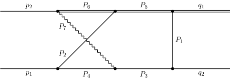
Figure 1: The non-planar double box topo5 which occurs, e.g., in virtual corrections to single top production at NNLO.

To illustrate the impact of the overhead reduction with the --bunch_size command-line option and the scaling with several nodes utilizing MPI, we chose the IBP reduction of the topology topo5 shown in Fig. 1 with the propagators

$$\begin{gathered}P_{1}=k_{1}^{2},\quad P_{2}=k_{2}^{2},\quad P_{3}=(q_{2}-k_{1})^{2},\quad P_{4}=(p_{1}-k_{2})^{2},\\ P_{5}=(q_{1}+k_{1})^{2}-m_{1}^{2},\quad P_{6}=(q_{1}+k_{1}-k_{2})^{2}-m_{1}^{2},\\ P_{7}=(q_{1}-p_{2}+k_{1}-k_{2})^{2}-m_{2}^{2},\quad P_{8}=(k_{1}-p_{1})^{2},\quad P_{9}=(k_{2}-q_{2}-p_{2})^{2},\end{gathered}$$ (6)

where $P_{8}$ and $P_{9}$ are auxiliary propagators. The scalar products of the external momenta can be expressed through the kinematical invariants by

$$\begin{gathered}p_{1}^{2}=p_{2}^{2}=q_{2}^{2}=0,\quad q_{1}^{2}=m_{1}^{2},\quad(p_{1}+p_{2})^{2}=s,\\ (q_{2}-p_{1})^{2}=t,\quad(q_{2}-p_{2})^{2}=m_{1}^{2}-s-t.\end{gathered}$$ (7)

This example can be found in examples/topo5. We perform the reduction with $r=7$ and $s=4$, which is sufficient for the virtual NNLO corrections to the amplitude of single top production. This results in about 1.6 million probes in total over four prime fields to complete the reduction. The runtime of the probes is dominated by the forward elimination with a contribution of 97 %. The calculations were performed on cluster nodes equipped with two Intel Xeon Platinum 8160 processors with 24 cores each and 192 GiB of RAM in total with hyper-threading disabled. On each node, we utilize all cores with the command line option ----parallel=48. topo5 has also been studied in Ref. [26] with emphasis on FireFly’s options.

In Tab. 1, we vary the maximal bunch size of FireFly with the command-line option --bunch_size as described in Sect. 3.1.

Table 1: Reduction of topo5 with $r=7$, $s=4$ utilizing FireFly, i.e. run_firefly: true, and the command-line option --bunch_size. As a comparison we present the algebraic reduction with Kira and Fermat, i.e. using run_triangular: true and run_back_substitution: true.

--bunch_size=	Runtime	Memory	CPU time per probe	CPU time for probes
1	18 h	40 GiB	1.73 s	95 %
2	14 h	41 GiB	1.30 s	94 %
4	11 h	46 GiB	1.00 s	93 %
8	10 h 15 min	51 GiB	0.91 s	92 %
16	9 h 45 min	63 GiB	0.85 s	92 %
32	9 h 30 min	82 GiB	0.84 s	92 %
64	9 h 30 min	116 GiB	0.83 s	92 %
Kira $\oplus$ Fermat	82 h	147 GiB	-	-

In general, the runtime decreases at the cost of additional memory, as expected. Increasing the bunch size from 1 to 2 costs about 1 GiB of additional RAM but already decreases the runtime by roughly 25 % by speeding up the average time to solve the system for one data point with pyRed by a similar percentage. The step to a bunch size of 4 again yields a runtime decrease of 20 % but already costs 5 GiB. In the following steps, the gain in runtime becomes smaller while the amount of additional memory required increases faster. Note that this example is mainly limited by the cost of computing probes with pyRed as shown in the last column, i.e. the internal calculations in FireFly only play a minor role. The share of the probes at the total CPU time for the reduction only decreases marginally.

In Tab. 2, we show the behaviour of the reduction of topo5 when using multiple nodes with Intel^® MPI [70].

Table 2: Reduction of topo5 with $r=7$ and $s=4$ utilizing FireFly, i.e. run_firefly: true, and multiple nodes with MPI. The speed-up is measured with respect to the reduction with bunch size 1 in Tab. 1. As a comparison we show the algebraic reduction with Kira and Fermat using run_triangular: true and run_back_substitution: true.

# nodes	Runtime	Speed-up	CPU efficiency
1	18 h	1.0	95 %
2	10 h 15 min	1.8	87 %
3	7 h 15 min	2.5	82 %
4	5 h 45 min	3.1	76 %
5	5 h 30 min	3.3	65 %
Kira $\oplus$ Fermat	82 h	-	-

The additional nodes are used as pure workers solving the IBP system with pyRed as described in Sect. 3.1. They require about 9 GiB of RAM. Doubling the number of cores yields a speed-up of 1.8. Using three nodes increases the speed-up to 2.5 and four to 3.1. Going to five nodes, the speed-up only marginally increases further to 3.3. Therefore, using even more nodes does not seem to be worthwhile for this example. However, the calculation is still limited by computation of the probes since the percentage of the CPU time for the probes does not vary much. On the other hand, the CPU efficiency drastically decreases, i.e. some of the cores are idle for some time during the calculation. This is due to the algorithms implemented in FireFly, which cannot process arbitrary probes. Instead, new probes are scheduled based on intermediate results. This is especially relevant for the first prime field, where the structure of the functions is not known yet. For more details, we refer to Refs. [24, 26].

Thus, both features can be used to significantly decrease the runtime of reductions which are limited by the evaluations of the probes. Bunches should be used if there is unused memory on the system, MPI if there are more computers or cluster nodes available. As already mentioned in Sect. 3.1, one should not use MPI when only using a single machine, mainly because one thread is reserved solely for communication. Of course, both features can also be combined if enough resources are available. It might also be worthwhile to monitor a long and difficult calculation and adapt the settings to the current status, e.g. by increasing the number of nodes when the prime field changes, because all probes are queued in the beginning, and decreasing the number when FireFly only interpolates the coefficients. In Sect. 4.4 we show an example which is mainly limited by the interpolation with FireFly and, thus, the potential speed-up by increasing the bunch size or by using MPI is relatively small, because both features effectively reduce the wall clock time to compute the probes.

4.2 Reducing the memory footprint with iterative reduction

The iterative reduction described in Sect. 3.3 can be used to reduce the memory footprint by setting master integrals to zero, either all except one master integral (“masterwise”) or all master integrals except those in one sector at a time (“sectorwise”). We again study topo5 as an example on the same machines with two Intel Xeon Platinum 8160 processors with 24 cores each and 192 GiB of RAM in total with hyper-threading disabled. As shown in Tab. 3, the required memory reduces by more than a factor of 4 for the reduction with FireFly when using the sectorwise iterative reduction.

Table 3: Sectorwise iterative reduction of topo5 with $r=7$ and $s=4$ utilizing FireFly, i.e. run_firefly: true, and --parallel=48.

Mode	Iterative	Runtime	Memory
Kira $\oplus$ FireFly	-	18 h	40 GiB
	sectorwise	33 h 15 min	9 GiB

However, the runtime increases by 80 % in this example.

4.3 Combining algebraic forward elimination with finite field reduction

Our next benchmark is an example from the study of conformal integrals in position space with the propagators

$$\begin{gathered}P_{1}=k_{1}^{2},\quad P_{2}=k_{2}^{2},\quad P_{3}=k_{3}^{2},\quad P_{4}=(p_{1}-k_{1})^{2},\quad P_{5}=(p_{1}-k_{2})^{2},\\ P_{6}=(p_{1}-k_{3})^{2},\quad P_{7}=(p_{2}-k_{1})^{2},\quad P_{8}=(p_{2}-k_{2})^{2},\quad P_{9}=(p_{2}-k_{3})^{2},\\ P_{10}=(k_{1}-k_{2})^{2},\quad P_{11}=(k_{1}-k_{3})^{2},\quad P_{12}=(k_{2}-k_{3})^{2}.\end{gathered}$$ (8)

The top-level sector is $4095$, i.e. all propagators may appear with positive powers. The scalar products of the external momenta can be expressed through new variables $z$ and $z_{b}$:

$$p_{1}^{2}=zz_{b},\quad p_{2}^{2}=1,\quad p_{1}p_{2}=(1-z)(1-z_{b}).$$ (9)

We chose $r=17$ and $s=0$ for the benchmark.

The reductions are performed on a machine with two Intel Xeon Gold 6138 with 20 cores each and 768 GiB of RAM in total with hyper-threading enabled. All cores including hyper-threading are utilised with the option --parallel=80. Tab. 4 compares different strategies for the reduction.

Table 4: Different strategies for the reduction of the topology defined by the propagators in Eq. (8). The reduction specific values are $r=17$ and $s=0$. The option run_initiate is used to initialise the system for all strategies, but is expensive enough to warrant a separate entry in the table.

Mode	Runtime	Memory	Probes	CPU time per probe	CPU time for probes
run_initiate	5 h 20 min	128 GiB	-	-	-
run_triangular + run_back_substitution	> 14 d	~ 540 GB	-	-	-
run_firefly: true	6 d 3 h	670 GiB	108500	370 s	100 %
run_triangular: sectorwise	36 min	4 GiB	-	-	-
run_firefly: back	4 h 54 min	35 GiB	108500	12.2 s	100 %

The initialization is already quite expensive, especially in terms of memory. The reduction with FireFly is completely limited by the calculation of the probes. Even though the total number is rather small compared to other problems, the 370 s for each probe are extremely expensive. 98 % of this time is spent on the forward elimination. However, the forward elimination can be performed in just 36 min by the algebraic mode of Kira. Using this result as starting point for FireFly significantly speeds up the probes to 12 s and, therefore, the whole reduction. Moreover, the memory footprint of the reduction improves significantly because the forward-solved system only consists of 572313 equations with 6144971 terms instead of 8922459 equations with 64009470 terms. However, the number of distinct coefficients increases from 205 to 983420 more complicated ones, because the forward elimination already partially solved the system. Thus, the time to evaluate these coefficients for each probe increases from 0.002 s to 3.3 s. Moreover, the time for the back substitution increases from 6.7 s to 8.9 s, because Kira and pyRed use different algorithms for the forward elimination and hence produce different triangular systems. Both increases are still completely irrelevant compared to the time saved by using the forward-solved system.

Thus, one should check whether the forward elimination can be computed algebraically to speed up the calculation with FireFly. However, usually the coefficients of the system are considerably more difficult after the forward elimination and are more expensive to parse and evaluate. This can completely offset the gain, especially for multi-scale problems.

4.4 Double-pentagon topology in five-light-parton scattering

The double-pentagon topology that appears in the amplitude of five-light-parton scattering at the two-loop level is illustrated in Fig. 2.

Figure 2: The double-pentagon topology for five-light-parton scattering. The propagators $P_{i}$ are defined in Eq. (11).

There are five external momenta $p_{1},\dots,p_{5}$ fulfilling $p_{i}^{2}=0$. All $p_{i}$ are assumed to be incoming, i.e. $\sum_{i}p_{i}=0$. The kinematical invariants are defined by

$$\begin{gathered}s_{12}=(p_{1}+p_{2})^{2},\quad s_{23}=(p_{2}+p_{3})^{2},\quad s_{34}=(p_{3}+p_{4})^{2},\\ s_{45}=(p_{4}+p_{5})^{2},\quad s_{51}=(p_{5}+p_{1})^{2}.\end{gathered}$$ (10)

Including $d$, the reduction of the double-pentagon topology is a six variable problem. By setting $s_{12}=1$ and restoring its dependence by dimensional analysis after the reduction, it can be reduced to a five variable problem.

The set of denominators describing the topology depicted in Fig. 2 is chosen as

$$\begin{gathered}P_{1}=l_{1}^{2},\quad P_{2}=(l_{1}+p_{1})^{2},\quad P_{3}=(l_{1}+p_{1}+p_{2})^{2},\quad P_{4}=l_{2}^{2},\\ P_{5}=(l_{2}+p_{3})^{2},\quad P_{6}=(l_{1}+l_{2}+p_{1}+p_{2}+p_{3})^{2},\quad P_{7}=(l_{1}+l_{2}-p_{4})^{2},\\ P_{8}=(l_{1}+l_{2})^{2},\quad P_{9}=(l_{2}+p_{1})^{2},\quad P_{10}=(l_{2}+p_{2})^{2},\quad P_{11}=(l_{2}+p_{4})^{2},\end{gathered}$$ (11)

where the last three entries are auxiliary denominators. The system of equations used in this reduction is taken from Ref. [30], which provides a system in block-triangular form. This form is much better suited for the reduction than a naive IBP system as generated, e.g., by Kira. The coefficients appearing in the system are further processed by FireFly to be cast in Horner form to optimize the evaluations.

We benchmark the reduction of all integrals including five scalar products. The reductions are performed on a machine with two Intel Xeon Gold 6138 with 20 cores each and 768 GiB of RAM in total with hyperthreading enabled. All cores including hyper-threading are utilised with the option --parallel=80. The integral selection is done using the option select_mandatory_list and we perform a numerical interpolation, i.e. run_firefly is set to true. Hence, $2268$ master integral coefficients have to be interpolated. Additionally, we set the maximum bunch size to $128$. Further simplifications are obtained by FireFly’s factor scan. In total $19222$ factors can be found of which $1930$ are attributed to $s_{23}$, $2176$ to $s_{34}$, $2046$ to $s_{45}$, $2306$ to $s_{51}$, and $10764$ to $d$. The results of this benchmark are shown in Tab. 5.

Table 5: Benchmark results for the reduction of the double-pentagon topology with the configuration described in the main text.

Runtime	Memory	Probes	CPU time per probe	CPU time for probes
12 d	540 GiB	38278000	0.37 s	25 %

The most complicated master integral coefficient has a maximum degree in the numerator of $87$ and in the denominator of $50$ thus yielding a dense bound of roughly $5.46\cdot 10^{7}$ possible non-zero monomials. Fortunately, many of these are zero such that only about $10^{7}$ monomials contribute. Without the scan for factors, the maximum degree of the denominator of the most complicated coefficient rises to $85$. The database of the reduction occupies $25$ GiB of disk space.

Although the number of required probes is comparably high, they can be computed relatively fast due to the block-triangular structure obtained in Ref. [30]. However, the interpolation of each coefficient is performed on a single thread and can become expensive in terms of runtime as the number of monomials usually rises factorially with the number of variables. Hence, in this example, the runtime for the interpolation is dominating. Note that there are two strategies to reduce the used memory of this calculation. On the one hand, the maximum bunch size can be reduced. On the other hand, the option iterative_reduction with masterwise or sectorwise can be used. By employing the latter option, the calculation can be distributed manually (sector- or masterwise) on several machines to obtain a runtime improvement in addition.

5 Installation

5.1 Obtaining Kira

A statically linked executable of Kira for Linux x86_64 is available from our web page at https://kira.hepforge.org. This executable has all optional features included except for MPI. If you require MPI, you must compile Kira yourself against the MPI version used on your computer cluster.

The source code of Kira is available from our Git repository at GitLab under the URL https://gitlab.com/kira-pyred/kira. To obtain the source code of the latest release version, clone the repository with

  git clone https://gitlab.com/kira-pyred/kira.git -b release

checking out the release branch. Release versions are also available as Git tags (e.g. kira-2.0). The master branch of the repository contains the latest pre-release version, receiving more frequent updates with new features and fixes. To obtain the source code of the latest pre-release version, clone the repository with

  git clone https://gitlab.com/kira-pyred/kira.git

checking out the master branch. Packages of the release versions as compressed Tar archives are available from https://kira.hepforge.org.

5.2 Prerequisites

Platform requirements
Linux x86_64 or macOS.

Compiler requirements
A C++ compiler supporting the C++14 standard and a C compiler supporting the C11 standard.

Build system requirements
Kira can either be built with the Meson build system [71] version 0.46 or later and Ninja [72], or with the Autotools build system [73].

We recommend to use the Meson build system. If Meson is not available on your system, it can be installed into your home directory as non-root user with

  pip3 install --user meson

(requires Python 3.5 or later). This will install Meson to ~/.local/bin.

The Ninja binary (and source code) is available from https://ninja-build.org.

Dependencies
Kira requires the following packages to be installed on the system:

• GiNaC [74, 75, 76], which itself requires CLN [77],

• zlib [78].

• Fermat [43] is required to run Kira.

If the Fermat executable is not found automatically at startup, or a specific Fermat installation should be used, the path to the Fermat executable can be provided via the environment variable FERMATPATH.

Depending on the enabled optional features of Kira, the following packages are required in addition:

• GMP [79] if FireFly is used,

• MPFR [80] if FLINT is used,

• an MPI [36] library (disabled by default) for parallelization on computer clusters,

• jemalloc [59] (disabled by default) for more efficient memory allocation.

The following dependencies can be automatically built and installed as subprojects with the Meson build system, i.e. if they are not found on the system, they will be built automatically along with Kira:

• yaml-cpp [81] (required),

• FireFly [26] (optional, enabled by default). If you decide to install FireFly manually, we recommend to use the version from the branch kira-2 of the Git repository at https://gitlab.com/firefly-library/firefly. This branch will remain compatible with Kira 2.0.

• FLINT [82] (optional, enabled by default). We recommend using FLINT, because it not only offers better performance for the finite field arithmetic, but is also required to enable some features of FireFly, most notably the factor scan.

If the Autotools build system is used, all enabled dependencies must be installed manually. If FireFly is not build as a subproject, to use FLINT and MPI, they must be enabled in FireFly’s CMake build system.

Note that GiNaC, CLN, yaml-cpp, and FireFly must have been compiled with the same compiler which is used to compile Kira. Otherwise the linking step will most likely fail. If you are using the system compiler, you can usually install GiNaC, CLN, and yaml-cpp via your system’s package manager. However, if you are using a different compiler, this usually means in practice that you also have to build these packages from source and, if installed with a non-default installation prefix, the environment variables C_PATH, LD_LIBRARY_PATH and PKG_CONFIG_PATH must be set accordingly.

5.3 Compiling Kira with the Meson build system

To build Kira with the Meson build system, Meson 0.46 (or later) and Ninja are required. If Meson and Ninja are not available on your system, see paragraph “Build system requirements” in Sect. 5.2.

To compile and install Kira, run

  meson --prefix=/install/path builddir
  cd builddir
  ninja
  ninja install

where builddir is the build directory. Specifying the installation prefix with --prefix is optional.

Build options

• -Dfirefly=false (default: true): Build without FireFly support.

• -Dflint=false (default: true): If FireFly is built as a subproject, disable FLINT.

• -Dmpi=true (default: false): If FireFly is built as a subproject, enable MPI. This is known to work best with OpenMPI [83, 84]. For performance reasons, we recommend MPICH [85], though.

• -Dcustom-mpi=<name>: If your MPI installation provides a pkg-config file, but is not found automatically with -Dmpi=true, pass the name of the MPI implementation as <name>, e.g. -Dcustom-mpi=mpich. Some systems don’t provide a pkg-config file for MPICH. In that case we recommend to install FireFly with its own CMake build system instead.

• -Djemalloc=true (default: false): Link with the jemalloc memory allocator [59]. This can lead to significantly increased performance, often by more than $20\,\%$ from our experience if FireFly is used. However, using jemalloc may not work on some systems, especially in combination with certain MPI implementations. Alternatively, to use jemalloc, one can set the environment variable LD_PRELOAD to point to jemalloc.so and export it.

To show the full list of available build options, run meson configure in the build directory.

Subprojects
If yaml-cpp or FireFly are not found on the system, per default they will be downloaded and built as Meson subprojects. If the option -Dflint=true (default) is set and FireFly is built as a subproject, also FLINT will be downloaded and built as a subproject if it is not found on the system.

The usage of subprojects can be controlled with the following options:

• --wrap-mode=nodownload: Do not download subprojects, but build them if already available (and not found on the system).

• --wrap-mode=nofallback: Do not build subprojects, even if the libraries are not found on the system.

• --wrap-mode=forcefallback: Build subprojects even if the libraries can be found on the system.

• --force-fallback-for=<deps>: Like forcefallback, but only for dependencies in the comma separated list <deps>. Overrides nofallback and forcefallback.

These options are only fully supported with Meson 0.49 or later. For details see
https://mesonbuild.com/Subprojects.html.

Note: Subprojects are not updated automatically. To update subprojects, run

  meson subprojects update

(requires Meson 0.49 or later). Git subprojects can of course also be manually updated by running git pull in the corresponding subproject directory (e.g. subprojects/firefly).

5.4 Compiling Kira with the Autotools build system

First run

  autoreconf -i

and then compile and install with

  ./configure --prefix=/install/path --enable-firefly=yes
  make
  make install

where the optional --prefix argument sets the installation prefix. Without the option --enable-firefly=yes, Kira will be built without FireFly support. Note that subproject installation is not supported with the Autotools build system, i.e. all dependencies must be installed manually.

6 Conclusions

In this article we presented the new version 2.0 of the Feynman integral reduction program Kira. The major new features introduced in this release are the reconstruction of final coefficients by means of finite field methods with the help of FireFly, and the parallelization of this procedure on computer clusters with MPI. Besides many minor improvements and extensions, the framework for the solution of user-provided systems of equations has been extended to support most features available for integration-by-parts reductions.

We reproduced benchmarks from previous Kira publications, showing significantly increased performance and reduced main memory consumption. Furthermore we provide new state-of-the-art benchmark points to demonstrate the effect of various newly added features on the computing resource requirements.

References

- [1] S. Amoroso et al., Les Houches 2019: Physics at TeV Colliders: Standard Model Working Group Report, in 11th Les Houches Workshop on Physics at TeV Colliders: PhysTeV Les Houches, 3, 2020, 2003.01700.
- [2] J. M. Henn, Multiloop Integrals in Dimensional Regularization Made Simple, Phys. Rev. Lett. 110 (2013) 251601 [1304.1806].
- [3] M. Argeri, S. Di Vita, P. Mastrolia, E. Mirabella, J. Schlenk, U. Schubert et al., Magnus and Dyson series for Master Integrals, JHEP 03 (2014) 082 [1401.2979].
- [4] A. von Manteuffel, E. Panzer and R. M. Schabinger, Computation of form factors in massless QCD with finite master integrals, Phys. Rev. D 93 (2016) 125014 [1510.06758].
- [5] F. Moriello, Generalised power series expansions for the elliptic planar families of Higgs + jet production at two loops, JHEP 01 (2020) 150 [1907.13234].
- [6] M. Hidding, DiffExp, a Mathematica package for computing Feynman integrals in terms of one-dimensional series expansions, 2006.05510.
- [7] J. Gluza, K. Kajda and D. A. Kosower, Towards a basis for planar two-loop integrals, Phys. Rev. D83 (2011) 045012 [1009.0472].
- [8] R. M. Schabinger, A new algorithm for the generation of unitarity-compatible integration by parts relations, JHEP 01 (2012) 077 [1111.4220].
- [9] H. Ita, Two-loop integrand decomposition into master integrals and surface terms, Phys. Rev. D94 (2016) 116015 [1510.05626].
- [10] J. Böhm, A. Georgoudis, K. J. Larsen, M. Schulze and Y. Zhang, Complete sets of logarithmic vector fields for integration-by-parts identities of Feynman integrals, Phys. Rev. D98 (2018) 025023 [1712.09737].
- [11] D. A. Kosower, Direct solution of integration-by-parts systems, Phys. Rev. D98 (2018) 025008 [1804.00131].
- [12] A. von Manteuffel, E. Panzer and R. M. Schabinger, Cusp and Collinear Anomalous Dimensions in Four-Loop QCD from Form Factors, Phys. Rev. Lett. 124 (2020) 162001 [2002.04617].
- [13] K. J. Larsen and Y. Zhang, Integration-by-parts reductions from unitarity cuts and algebraic geometry, Phys. Rev. D93 (2016) 041701 [1511.01071].
- [14] J. Böhm, A. Georgoudis, K. J. Larsen, H. Schönemann and Y. Zhang, Complete integration-by-parts reductions of the non-planar hexagon-box via module intersections, JHEP 09 (2018) 024 [1805.01873].
- [15] D. Bendle, J. Böhm, W. Decker, A. Georgoudis, F.-J. Pfreundt, M. Rahn et al., Integration-by-parts reductions of Feynman integrals using Singular and GPI-Space, JHEP 02 (2020) 079 [1908.04301].
- [16] P. Mastrolia and S. Mizera, Feynman integrals and intersection theory, JHEP 02 (2019) 139 [1810.03818].
- [17] H. Frellesvig, F. Gasparotto, S. Laporta, M. K. Mandal, P. Mastrolia, L. Mattiazzi et al., Decomposition of Feynman integrals on the maximal cut by intersection numbers, JHEP 05 (2019) 153 [1901.11510].
- [18] H. Frellesvig, F. Gasparotto, M. K. Mandal, P. Mastrolia, L. Mattiazzi and S. Mizera, Vector Space of Feynman Integrals and Multivariate Intersection Numbers, Phys. Rev. Lett. 123 (2019) 201602 [1907.02000].
- [19] S. Weinzierl, On the computation of intersection numbers for twisted cocycles, 2002.01930.
- [20] H. Frellesvig, F. Gasparotto, S. Laporta, M. K. Mandal, P. Mastrolia, L. Mattiazzi et al., Decomposition of Feynman Integrals by Multivariate Intersection Numbers, 2008.04823.
- [21] A. von Manteuffel and R. M. Schabinger, A novel approach to integration by parts reduction, Phys. Lett. B744 (2015) 101 [1406.4513].
- [22] T. Peraro, Scattering amplitudes over finite fields and multivariate functional reconstruction, JHEP 12 (2016) 030 [1608.01902].
- [23] A. V. Smirnov and F. S. Chukharev, FIRE6: Feynman Integral REduction with modular arithmetic, Comput. Phys. Commun. 247 (2020) 106877 [1901.07808].
- [24] J. Klappert and F. Lange, Reconstructing rational functions with FireFly, Comput. Phys. Commun. 247 (2020) 106951 [1904.00009].
- [25] T. Peraro, FiniteFlow: multivariate functional reconstruction using finite fields and dataflow graphs, JHEP 07 (2019) 031 [1905.08019].
- [26] J. Klappert, S. Y. Klein and F. Lange, Interpolation of dense and sparse rational functions and other improvements in FireFly, Comput. Phys. Commun. 264 (2021) 107968 [2004.01463].
- [27] X. Liu, Y.-Q. Ma and C.-Y. Wang, A systematic and efficient method to compute multi-loop master integrals, Phys. Lett. B779 (2018) 353 [1711.09572].
- [28] X. Liu and Y.-Q. Ma, Determining arbitrary Feynman integrals by vacuum integrals, Phys. Rev. D99 (2019) 071501 [1801.10523].
- [29] Y. Wang, Z. Li and N. ul Basat, Direct reduction of multiloop multiscale scattering amplitudes, Phys. Rev. D 101 (2020) 076023 [1901.09390].
- [30] X. Guan, X. Liu and Y.-Q. Ma, Complete reduction of integrals in two-loop five-light-parton scattering amplitudes, Chin. Phys. C 44 (2020) 093106 [1912.09294].
- [31] S. Laporta, High-precision calculation of multiloop Feynman integrals by difference equations, Int.J.Mod.Phys. A15 (2000) 5087 [hep-ph/0102033].
- [32] C. Anastasiou and A. Lazopoulos, Automatic integral reduction for higher order perturbative calculations, JHEP 07 (2004) 046 [hep-ph/0404258].
- [33] A. von Manteuffel and C. Studerus, Reduze 2 – Distributed Feynman Integral Reduction, 1201.4330.
- [34] A. V. Smirnov, FIRE5: A C++ implementation of Feynman Integral REduction, Comput. Phys. Commun. 189 (2015) 182 [1408.2372].
- [35] P. Maierhöfer, J. Usovitsch and P. Uwer, Kira—A Feynman integral reduction program, Comput. Phys. Commun. 230 (2018) 99 [1705.05610].
- [36] MPI Forum, Message Passing Interface, https://www.mpi-forum.org.
- [37] R. V. Harlander, Y. Kluth and F. Lange, The two-loop energy–momentum tensor within the gradient-flow formalism, Eur. Phys. J. C78 (2018) 944 [1808.09837].
- [38] J. Artz, R. V. Harlander, F. Lange, T. Neumann and M. Prausa, Results and techniques for higher order calculations within the gradient-flow formalism, JHEP 06 (2019) 121 [1905.00882].
- [39] R. V. Harlander, F. Lange and T. Neumann, Hadronic vacuum polarization using gradient flow, JHEP 08 (2020) 109 [2007.01057].
- [40] F. V. Tkachov, A theorem on analytical calculability of 4-loop renormalization group functions, Phys. Lett. B 100 (1981) 65.
- [41] K. G. Chetyrkin and F. V. Tkachov, Integration by parts: The algorithm to calculate -functions in 4 loops, Nucl. Phys. B192 (1981) 159.
- [42] T. Gehrmann and E. Remiddi, Differential equations for two-loop four-point functions, Nucl. Phys. B580 (2000) 485 [hep-ph/9912329].
- [43] R. H. Lewis, Computer Algebra System Fermat, https://home.bway.net/lewis.
- [44] M. Kauers, Fast Solvers for Dense Linear Systems, Nucl. Phys. B Proc. Suppl. 183 (2008) 245.
- [45] P. Kant, Finding linear dependencies in integration-by-parts equations: A Monte Carlo approach, Comput. Phys. Commun. 185 (2014) 1473 [1309.7287].
- [46] J. de Kleine, M. Monagan and A. Wittkopf, Algorithms for the Non-monic Case of the Sparse Modular GCD Algorithm, Proc. Int. Symp. Symbolic Algebraic Comp. 2005 (2005) 124.
- [47] R. Zippel, Probabilistic algorithms for sparse polynomials, Symbolic Algebraic Comp. EUROSAM 1979 (1979) 216.
- [48] M. Ben-Or and P. Tiwari, A Deterministic Algorithm for Sparse Multivariate Polynomial Interpolation, Proc. ACM Symp. Theory Comp. 20 (1988) 301.
- [49] E. Kaltofen and Lakshman Y., Improved Sparse Multivariate Polynomial Interpolation Algorithms, Symbolic Algebraic Comp. ISSAC 1988 (1989) 467.
- [50] R. Zippel, Interpolating Polynomials from their Values, J. Symb. Comp. 9 (1990) 375.
- [51] E. Kaltofen, W.-s. Lee and A. A. Lobo, Early Termination in Ben-Or/Tiwari Sparse Interpolation and a Hybrid of Zippel’s Algorithm, Proc. Int. Symp. Symbolic Algebraic Comp. 2000 (2000) 192.
- [52] E. Kaltofen and W.-s. Lee, Early termination in sparse interpolation algorithms, J. Symb. Comp. 36 (2003) 365.
- [53] A. Cuyt and W.-s. Lee, Sparse interpolation of multivariate rational functions, Theor. Comp. Sci. 412 (2011) 1445.
- [54] P. S. Wang, A p-adic Algorithm for Univariate Partial Fractions, Proc. ACM Symp. Symbolic Algebraic Comp. 1981 (1981) 212.
- [55] M. Monagan, Maximal Quotient Rational Reconstruction: An Almost Optimal Algorithm for Rational Reconstruction, Proc. Int. Symp. Symbolic Algebraic Comp. 2004 (2004) 243.
- [56] J. von zur Gathen and J. Gerhard, Modern Computer Algebra. Cambridge University Press, third ed., 2013, 10.1017/CBO9781139856065.
- [57] R. A. DeMillo and R. J. Lipton, A probabilistic remark on algebraic program testing, Inf. Process. Lett. 7 (1978) 193.
- [58] J. T. Schwartz, Fast Probabilistic Algorithms for Verification of Polynomial Identities, J. ACM 27 (1980) 701.
- [59] J. Evans et al., jemalloc memory allocator, http://jemalloc.net.
- [60] P. Maierhöfer and J. Usovitsch, Kira 1.1 Release Notes, https://kira.hepforge.org/downloads?f=papers/kira-release-notes-1.1.pdf.
- [61] P. Maierhöfer and J. Usovitsch, Kira 1.2 Release Notes, 1812.01491.
- [62] C. Sabbah, Lieu des pôles d’un système holonome d’équations aux différences finies, Bulletin de la Société Mathématique de France 120 (1992) 371.
- [63] A. V. Smirnov and V. A. Smirnov, How to choose master integrals, Nucl. Phys. B 960 (2020) 115213 [2002.08042].
- [64] J. Usovitsch, Factorization of denominators in integration-by-parts reductions, 2002.08173.
- [65] C. G. Papadopoulos, D. Tommasini and C. Wever, Two-loop master integrals with the simplified differential equations approach, JHEP 01 (2015) 072 [1409.6114].
- [66] M. Hidding and F. Moriello, All orders structure and efficient computation of linearly reducible elliptic Feynman integrals, JHEP 01 (2019) 169 [1712.04441].
- [67] C. G. Papadopoulos and C. Wever, Internal reduction method for computing Feynman integrals, JHEP 02 (2020) 112 [1910.06275].
- [68] A. G. Grozin, Heavy Quark Effective Theory, Springer Tracts Mod. Phys. 201 (2004) 1.
- [69] H. Frellesvig, R. Bonciani, V. Del Duca, F. Moriello, J. Henn and V. Smirnov, Non-planar two-loop Feynman integrals contributing to Higgs plus jet production, PoS LL2018 (2018) 076.
- [70] Intel Corporation, Intel ® MPI Library, https://software.intel.com/content/www/us/en/develop/tools/mpi-library.html.
- [71] J. Pakkanen, The Meson Build system, https://mesonbuild.com.
- [72] E. Martin, Ninja, https://ninja-build.org.
- [73] GNU Project, Autotools, https://www.gnu.org/software/automake/manual/html_node/Autotools-Introduction.html.
- [74] C. Bauer, A. Frink, R. B. Kreckel et al., GiNaC is not a CAS, https://www.ginac.de.
- [75] C. Bauer, A. Frink and R. Kreckel, Introduction to the GiNaC Framework for Symbolic Computation within the C++ Programming Language, J. Symb. Comput. 33 (2002) 1 [cs/0004015].
- [76] J. Vollinga, GiNaC: Symbolic computation with C++, Nucl. Instrum. Meth. A559 (2006) 282 [hep-ph/0510057].
- [77] B. Haible and R. B. Kreckel, CLN - Class Library for Numbers, https://www.ginac.de/CLN.
- [78] J.-l. Gailly and M. Adler, zlib, https://zlib.net.
- [79] GNU Project, GNU Multiple Precision Arithmetic Library, https://gmplib.org.
- [80] GNU Project, GNU Multiple Precision Floating-Point Reliable Library, https://www.mpfr.org.
- [81] J. Beder et al., yaml-cpp, https://github.com/jbeder/yaml-cpp.
- [82] W. Hart et al., FLINT: Fast Library for Number Theory, http://www.flintlib.org.
- [83] E. Gabriel et al., Open Source High Performance Computing, https://www.open-mpi.org.
- [84] E. Gabriel et al., Open MPI: Goals, Concept, and Design of a Next Generation MPI Implementation, Adv. Parallel Virtual Machine Message Passing Interface. EuroPVM/MPI 2004 (2004) 97.
- [85] W. Gropp et al., MPICH, https://www.mpich.org.
- [86] J. P. Ellis, Tikz-Feynman: Feynman diagrams with Tikz, Comput. Phys. Commun. 210 (2017) 103 [1601.05437].