Hadronic vacuum polarization using gradient flow

Abstract

The gradient-flow operator product expansion for QCD current correlators including operators up to mass dimension four is calculated through NNLO. This paves an alternative way for efficient lattice evaluations of hadronic vacuum polarization functions. In addition, flow-time evolution equations for flowed composite operators are derived. Their explicit form for the non-trivial dimension-four operators of QCD is given through order $\alpha_{s}^{3}$.

1 Introduction

The vacuum polarization functions for (axial-)vector and (pseudo-)scalar particles are among the most important objects when studying QCD. On the one hand, this is because their imaginary part is directly related to physical observables such as the decay rates of the $Z$- or the Higgs boson, or the hadronic R-ratio. If the characteristic energy scale is far above the QCD scale, a perturbative evaluation of the polarization functions is sufficient in these cases to arrive at high-precision results (see, e.g., Ref. [1]).

But VPFs also contribute indirectly to physical observables such as anomalous magnetic moments[Jegerlehner:2017gek, Aoyama:2020ynm], the definition of short-distance quark masses[Chetyrkin:2010ic], or hadronic contributions to the QED coupling [crivellin:2020, Keshavarzi:2020bfy]. These applications involve an integration of the VPFs over the non-perturbative regime, which is typically achieved with the help of experimental data and dispersion relations. Only very recently, first-principle lattice calculations have become competitive with these dispersive approaches. In the case of the hadronic vacuum polarization contribution to the muon’s anomalous magnetic moment, the two approaches turn out to lead to incompatible results[Borsanyi:2020mff]. It would therefore be highly desirable to have additional independent first-principle calculations of the VPF.

About ten years ago, the gradient-flow formalism (GFF) was suggested as a mechanism to improve the efficiency of lattice calculations[Luscher:2010iy, Luscher:2011bx, Luscher:2013cpa] (see also Refs. [Narayanan:2006rf, Luscher:2009eq]). Since then, it has become a standard for the scale-setting procedure[Borsanyi:2012zs, Sommer:2014mea]. However, also other applications of the GFF have been studied, among them a new way to determine the energy-momentum tensor on the lattice. The underlying idea in this case is the small-flow-time expansion of composite operators[Luscher:2011bx], leading to the flowed Operator Product Expansion (OPE) (also named smeared OPE in Ref. [Monahan:2014tea, Monahan:2015lha]), where the regular operators are replaced by operators taken at finite flow time. Its main advantages with respect to (w.r.t.) the regular OPE is the absence of operator mixing, and the improved efficiency of the evaluation of operator matrix elements. The translation of the regular to the flowed operators can be done perturbatively. For the energy-momentum tensor, it is available through next-to-next-to-leading order (NNLO)[Suzuki:2013gza, Makino:2014taa, Harlander:2018zpi]. Quite recently, the small-flow-time expansion was applied at next-to-leading order (NLO) to CP-violating operators[Rizik:2020naq], and to four-quark operators[Suzuki:2020zue].

In this paper, we present the flowed OPE for the time-ordered product of two currents through NNLO QCD. Taking the vacuum expectation value (VEV) leads to the VPF. This should thus allow for an alternative first-principle evaluation of VPFs on the lattice. In addition, we derive a general logarithmic flow-time evolution equation for flowed operators which resembles the renormalization group (RG) equation of regular operators.

The remainder of this paper is organized as follows. Section 2 introduces the regular OPE of current correlators with operators up to mass dimension four. This includes the renormalization of these operators as well as an overview of the literature which provides the corresponding perturbative Wilson coefficients. (The coefficients for the dimension-four operators for various currents are reproduced in Appendix B.) The transition to the flowed OPE is presented in Sect. 3. Section 4 describes the calculation of the mixing matrix between regular and flowed operators in the small-flow-time limit. While a large part of this mixing matrix is already known [Harlander:2018zpi] and recollected in Appendix C, the missing components require higher order mass terms of the VEV of the flowed dimension-four operators and their renormalization with the help of the vacuum-energy renormalization constant. These results complete the ingredients required for the flowed OPE of the VPF through NNLO. In Sect. 5, we derive a logarithmic evolution equation from the generic flow-time dependence of the mixing matrix. Section 6 presents our conclusions and gives a short outlook on possible extensions of this work.

2 Current-current correlators

Our results are presented for a general non-Abelian gauge theory based on a simple compact Lie group with $n_{\text{f}}$ quark fields $\psi_{1},\ldots,\psi_{n_{\text{f}}}$ in the fundamental representation, of which the first $n_{\text{h}}$ are degenerate with mass $m$, while the remaining $n_{\text{l}}$ are massless. The generators $T^{a}$ of the fundamental representation are normalized as $\text{Tr}(T^{a}T^{b})=-T_{\text{R}}\delta^{ab}$, and the structure constants $f^{abc}$ are defined through the Lie algebra $[T^{a},T^{b}]=f^{abc}T^{c}$. The dimensions of the fundamental and the adjoint representation are $n_{\text{c}}$ and $n_{\text{A}}$, respectively, and their quadratic Casimir eigenvalues are denoted by $C_{\text{F}}$ and $C_{\text{A}}$. For SU$(N)$, it is

$$\begin{split}n_{\text{c}}=N\,,\qquad n_{\text{A}}=N^{2}-1\,,\qquad C_{\text{F}}=T_{\text{R}}\frac{N^{2}-1}{N}\,,\qquad C_{\text{A}}=2T_{\text{R}}N\,,\end{split}$$ (2.1)

and QCD is recovered for $T_{\text{R}}=1/2$ and $N=3$, i.e. $C_{\text{F}}=4/3$ and $C_{\text{A}}=3$. For brevity, we often use “QCD” also to refer to the more general gauge theory in the following.

2.1 Operator product expansion

The role of the perturbative and the non-perturbative regime of VPFs can be made most explicit through the OPE (see, e.g., Ref. [Dominguez:2014vca]):

$$\begin{split}T(Q)\equiv\int\mathrm{d}^{4}x\,e^{iQx}\langle Tj(x)j(0)\rangle\stackrel{{\scriptstyle Q^{2}\to\infty}}{{\sim}}\sum_{k,n}C^{(k),\text{{B}}}_{n}(Q)\langle O^{(k)}_{n}(x=0)\rangle\,,\end{split}$$ (2.2)

where $j(x)$ generically stands for a scalar, pseudo-scalar, vector, axial-vector, or tensor current, and $k$ labels the mass dimension. Fig. 1 shows sample Feynman diagrams which arise from the perturbative evaluation of the current correlator in Eq. (2.2). In the following, we only consider the so-called non-singlet diagrams, where the currents are connected by a common quark line. An example for a singlet-diagram, on the other hand, is shown in Fig. 1 (e).

(a) (b)

(c) (d) (e)

Figure 1: Sample diagrams contributing to the perturbative calculation of the VPF, i.e., the left-hand side of Eq. (2.2). The currents are symbolized by wavy lines, gluons by spirals. We consider the case where $n_{\text{l}}$ quarks are massless (thin straight lines), and $n_{\text{h}}$ quarks are degenerate with mass $m$ (thick straight lines). (a) One-loop contribution for non-diagonal currents; (b-e) sample three-loop diagrams for diagonal currents. In (d), the currents couple to massless quarks. (e) is a “singlet” diagram. All diagrams in this paper were produced with the help of FeynGame[Harlander:2020cyh].

The coefficients $C_{n}^{(k),\text{{B}}}$ on the right-hand side of Eq. (2.2) depend on the quantum numbers of the current and may thus carry Lorentz indices. Apart from the explicit results for specific currents in Appendix B, we suppress these indices throughout the paper. We furthermore assume that, upon transition from the left- to the right-hand side, possible global divergences are subtracted off of $T(Q)$.

Up to mass dimension two, the only operators of QCD which contribute to physical matrix elements are proportional to unity, i.e.,

$$\begin{split}O^{(0)}_{1}\equiv O^{(0)}=\mathds{1}\,,\qquad O^{(2)}_{1}\equiv O^{(2)}=m_{\text{{B}}}^{2}\,\mathds{1}\,,\end{split}$$ (2.3)

where $m_{\text{{B}}}$ is the bare mass of the $n_{\text{h}}$ degenerate massive quarks. This means that

$$\begin{split}C_{1}^{(0)}\equiv C^{(0)}\equiv C^{(0),\text{{B}}}\,,\qquad C_{1}^{(2)}\equiv C^{(2)}\equiv Z_{m}^{2}C^{(2),\text{{B}}}\end{split}$$ (2.4)

are ultra-violet (UV)-finite, where $Z_{m}$ is the renormalization constant of the quark mass defined in Appendix A.

At mass dimension four, we choose the following basis of operators (the space-time argument is suppressed in most of what follows):

$$\begin{split}O^{(4)}_{1}\equiv O_{1}&=\frac{1}{g_{\text{{B}}}^{2}}F^{a}_{\mu\nu}F^{a}_{\mu\nu}\,,\\ O^{(4)}_{2}\equiv O_{2}&=\sum_{q=1}^{n_{\text{f}}}\bar{\psi}_{q}\overleftrightarrow{\not{D}}\psi_{q}\,,\\ O^{(4)}_{3}\equiv O_{3}&=m_{\text{{B}}}^{4}\,,\end{split}$$ (2.5)

where

$$\begin{split}F^{a}_{\mu\nu}&=\partial_{\mu}A^{a}_{\nu}-\partial_{\nu}A^{a}_{\mu}+f^{abc}A_{\mu}^{b}A_{\nu}^{c}\,,\qquad\overleftrightarrow{D}\!_{\mu}=\partial_{\mu}-\overleftarrow{\partial}_{\mu}+2A^{a}_{\mu}T^{a}\,,\end{split}$$ (2.6)

with the regular (as opposed to “flowed”, see Sect. 3) quark and gluon fields $\psi_{q}(x)$ and $A^{a}_{\mu}(x)$, respectively, and the bare coupling $g_{\text{{B}}}$.

We employ Euclidean space-time, but translation of the intermediate formulas and the final results to Minkowski space is possible without difficulty. Working in

$$\begin{split}d=4-2\epsilon\end{split}$$ (2.7)

space-time dimensions, the mass dimensions of $O_{1}$ and $O_{2}$ are actually equal to $d$, while that of $O_{3}$ is equal to 4. Higher dimensional operators are neglected in the following.

The set in Eq. (2.5) does not contain gauge dependent operators, or operators that vanish due to the equations of motion when acting on physical states, since they are irrelevant for the scope of this paper. In fact, in this respect the upper limit of the sum over $q$ in $O_{2}$ could be replaced by $n_{\text{h}}$, because the terms with massless quarks vanish on-shell. For the same reason, one could use $O_{2}^{\prime}\equiv-2m_{\text{{B}}}\sum_{q=1}^{n_{\text{h}}}\bar{\psi}_{q}\psi_{q}$ instead of $O_{2}$ in the definition of the operator basis (2.5). Other choices are possible as well, but the basis in Eq. (2.5) is particularly suitable for our purposes, because it is most directly related to the operator basis used in Refs. [Makino:2014taa, Makino:2018rys, Harlander:2018zpi].

Matrix elements of the dimension-four operators are divergent in general. However, one may define “renormalized operators” $O_{n}^{\text{{R}}}$ as linear combinations among them, for which physical matrix elements become finite:

$$\begin{split}O^{\text{{R}}}_{n}=\sum_{k}Z_{nk}\,O_{k}\,.\end{split}$$ (2.8)

Analogously, one defines renormalized coefficient functions through the condition

$$\begin{split}\sum_{n}C_{n}^{\text{{B}}}O_{n}\stackrel{{\scriptstyle!}}{{=}}\sum_{n}C_{n}O^{\text{{R}}}_{n}\quad\Rightarrow\quad C_{n}=\sum_{m}C^{\text{{B}}}_{m}(Z^{-1})_{mn}\,,\end{split}$$ (2.9)

where $C^{\text{{B}}}_{n}\equiv C_{n}^{(4),\text{{B}}}$, cf. Eqs. (2.2) and (2.5). It is well known that, since the operators of Eq. (2.5) are part of the QCD Lagrangian, the renormalization matrix $Z$ can be expressed in terms of the anomalous dimensions of QCD[Spiridonov:1984br, Spiridonov:1988md]:

$$\begin{split}Z&=\left(\begin{matrix}Z_{2\times 2}&\vec{Z}_{3}\\[5.0pt] \vec{0}^{\,T}&Z_{m}^{-4}\end{matrix}\right)\,,\quad\mbox{where}\quad Z_{2\times 2}=\left(\begin{matrix}-\epsilon/\beta_{\epsilon}&-2\gamma_{m}/\beta_{\epsilon}\\ 0&1\end{matrix}\right)\,,\\ \vec{Z}_{3}&=4\hat{\mu}^{-2\epsilon}Z_{m}^{-4}\left(\begin{matrix}\displaystyle a_{s}\frac{\partial}{\partial a_{s}}Z_{0}\\[10.00002pt] 2\,Z_{0}\end{matrix}\right)\,,\quad\hat{\mu}\equiv\frac{\mu}{\sqrt{4\pi}}e^{\gamma_{\text{E}}/2}\,.\end{split}$$ (2.10)

The ’t Hooft mass $\mu$ ensures that each renormalized operator $O_{n}^{\text{{R}}}$ in Eq. (2.8) has the same mass dimension as the corresponding bare one, and $\hat{\mu}$ appears because we will adopt the $\overline{\mbox{{MS}}}$ scheme by default ($\gamma_{\text{E}}=-\Gamma^{\prime}(1)=0.577216\ldots$). We also introduced the quantity $a_{s}=\alpha_{s}/\pi=g^{2}/(4\pi^{2})$ here, where $g$ is the renormalized strong coupling in the $\overline{\mbox{{MS}}}$ scheme. $Z_{0}$ is the $\overline{\mbox{{MS}}}$ renormalization constant for the vacuum energy[Spiridonov:1988md]. It is given in Appendix A, together with the anomalous quark mass dimension $\gamma_{m}$ and the $d$-dimensional beta function $\beta_{\epsilon}$.

2.2 Coefficient functions

The OPE form of the current correlators is usually inconvenient for their perturbative evaluation. Instead, one rather evaluates the l.h.s. of Eq. (2.2) directly by calculating the relevant two-point functions to the appropriate order. The exact analytical result for general quark masses is known at the two-loop level[Kallen:1955fb, Broadhurst:1981jk, Kniehl:1989yc, Djouadi:1993ss], while higher orders up to the four-loop level have been reconstructed by combining various kinematical limits[Broadhurst:1993mw, Fleischer:1994ef, Broadhurst:1994qj, Baikov:1995ui, Chetyrkin:1995ii, Chetyrkin:1997mb, Chetyrkin:1998ix, Hoang:2008qy, Kiyo:2009gb, Greynat:2010kx, Greynat:2011zp], or through integral reduction[Tkachov:1981wb, Chetyrkin:1981qh, Laporta:2001dd] and subsequent numerical evaluation of the resulting master integrals[Maier:2017ypu].

Since the dimension-zero and -two operators in Eq. (2.2) are proportional to unity, the coefficients $C^{(0)}$ and $C^{(2)}$ are immediately determined from the small-mass expansion of these perturbative results for the VPF. They are thus known up to the four-loop level at the moment[Chetyrkin:1979bj, Dine:1979qh, Celmaster:1979dm, Gorishnii:1986pz, Chetyrkin:1997qi, Harlander:1997kw, Harlander:1997xa, Baikov:2004ku, Baikov:2009uw].

The Wilson coefficients $C_{n}$ of the dimension-four operators, on the other hand, require a dedicated calculation which keeps track of the contributions from the individual operators. This has been done through ${\cal O}(a_{s}^{3})$ for $C_{1}$ and $C_{2}$, and through ${\cal O}(a_{s}^{2})$ for $C_{3}$ in Refs. [Chetyrkin:1985kn, Chetyrkin:1994ex, Chetyrkin:2000zk, Harlander:diss]. For the purpose of this paper, only the ${\cal O}(a_{s}^{2})$ results are required. For completeness, we include them in Appendix B.

3 Flowed operator product expansion

Having introduced the setup in the “regular” theory, we now translate this to the flowed OPE for the current correlators.

3.1 Flowed operators

We introduce the flowed operators as

$$\begin{split}\tilde{O}_{1}(t,x)&=\frac{Z_{s}}{g_{\text{{B}}}^{2}}\,G^{a}_{\mu\nu}(t,x)G^{a}_{\mu\nu}(t,x)=\frac{\hat{\mu}^{-2\epsilon}}{g^{2}}\,G^{a}_{\mu\nu}(t,x)G^{a}_{\mu\nu}(t,x)\,,\\ \tilde{O}_{2}(t,x)&=\mathring{Z}_{\chi}\sum_{q=1}^{n_{\text{f}}}\bar{\chi}_{q}(t,x)\overleftrightarrow{\not{\mathcal{D}}}(t,x)\chi_{q}(t,x)\,,\\[5.0pt] \tilde{O}_{3}(t,x)&=m^{4}\,,\end{split}$$ (3.1)

where

$$\begin{split}\overleftrightarrow{\mathcal{D}}\!_{\mu}={\mathcal{D}}\!_{\mu}-\overleftarrow{\mathcal{D}}\!_{\mu}\,,\qquad{\mathcal{D}}\!_{\mu}=\partial_{\mu}+B^{a}_{\mu}T^{a}\,,\qquad\overleftarrow{\mathcal{D}}\!_{\mu}=\overleftarrow{\partial}_{\mu}-B^{a}_{\mu}T^{a}\,.\end{split}$$ (3.2)

The flowed gauge and quark fields $B^{a}_{\mu}=B^{a}_{\mu}(x,t)$ and $\chi_{q}=\chi_{q}(x,t)$ obey the equations[Luscher:2010iy, Luscher:2013cpa]

$$\begin{split}\partial_{t}B^{a}_{\mu}&=\mathcal{D}^{ab}_{\nu}G^{b}_{\nu\mu}+\kappa\mathcal{D}^{ab}_{\mu}\partial_{\nu}B^{b}_{\nu}\,,\\ \partial_{t}\chi_{q}&=\Delta\chi_{q}-\kappa\partial_{\mu}B^{a}_{\mu}T^{a}\chi_{q}\,,\\ \partial_{t}\bar{\chi}_{q}&=\bar{\chi}_{q}\overleftarrow{\Delta}+\kappa\bar{\chi}_{q}\partial_{\mu}B^{a}_{\mu}T^{a}\,,\end{split}$$ (3.3)

with the initial conditions

$$\begin{split}B^{a}_{\mu}(t=0,x)=A^{a}_{\mu}(x)\,,\qquad\chi_{q}(t=0,x)=\psi_{q}(x)\,,\quad q\in\{1,\ldots n_{\text{f}}\}\,.\end{split}$$ (3.4)

Here we used the flowed covariant derivative in the adjoint representation,

$$\begin{split}\mathcal{D}_{\mu}^{ab}=\delta^{ab}\partial_{\mu}-f^{abc}B_{\mu}^{c}\,,\end{split}$$ (3.5)

and the flowed Laplace operators

$$\begin{split}\Delta=\mathcal{D}_{\mu}\mathcal{D}_{\mu}\,,\qquad\overleftarrow{\Delta}=\overleftarrow{\mathcal{D}}_{\mu}\overleftarrow{\mathcal{D}}_{\mu}\,,\end{split}$$ (3.6)

where the flowed covariant derivatives in the fundamental representation are given in Eq. (3.2). For our three-loop calculations, we set the gauge parameter $\kappa=1$ in Eq. (3.3), because this simplifies the intermediate expressions. All our results are independent of this choice though.

$\mathring{Z}_{\chi}$ is the non-minimal renormalization constant for the flowed quark fields $\chi_{q}$, defined by the all-order condition[Makino:2014taa]

$$\begin{split}\langle\tilde{O}_{2}(t)\rangle\bigg{|}_{m=0}\equiv-\frac{2n_{\text{c}}n_{\text{f}}}{(4\pi t)^{2}}\,,\end{split}$$ (3.7)

where $\langle\cdot\rangle$ denotes the VEV. It reads

$$\begin{split}\mathring{Z}_{\chi}=\zeta_{\chi}\,Z_{\chi}\,,\end{split}$$ (3.8)

where $Z_{\chi}$ is the $\overline{\mbox{{MS}}}$ part,

$$\begin{split}Z_{\chi}&=1+a_{s}\frac{\gamma_{\chi,0}}{2\epsilon}+a_{s}^{2}\left[\frac{\gamma_{\chi,0}}{4\epsilon^{2}}\left(\frac{\gamma_{\chi,0}}{2}-\beta_{0}\right)+\frac{\gamma_{\chi,1}}{4\epsilon}\right]+{\cal O}(a_{s}^{3})\,,\end{split}$$ (3.9)

and

$$\begin{split}\zeta_{\chi}&=1+a_{s}\left(\frac{\gamma_{\chi,0}}{2}L_{\mu t}-\frac{3}{4}C_{\text{F}}\ln 3-C_{\text{F}}\ln 2\right)\\ &\qquad+a_{s}^{2}\Bigg{\{}\frac{\gamma_{\chi,0}}{4}\left(\beta_{0}+\frac{\gamma_{\chi,0}}{2}\right)L_{\mu t}^{2}+\Big{[}\frac{\gamma_{\chi,1}}{2}-\frac{\gamma_{\chi,0}}{2}\left(\beta_{0}+\frac{\gamma_{\chi,0}}{2}\right)\ln 3\\ &\qquad\qquad-\frac{2}{3}\gamma_{\chi,0}\left(\beta_{0}+\frac{\gamma_{\chi,0}}{2}\right)\ln 2\Big{]}L_{\mu t}+\frac{c_{\chi}^{(2)}}{16}\Bigg{\}}+{\cal O}(a_{s}^{3})\,.\end{split}$$ (3.10)

The short-hand notation

$$\begin{split}L_{\mu t}=\ln\frac{\mu^{2}}{\mu_{t}^{2}}\,,\qquad\mu_{t}=\frac{1}{\sqrt{2te^{\gamma_{\text{E}}}}}\end{split}$$ (3.11)

reflects our choice of the “central” renormalization scale $\mu_{t}$ [Harlander:2018zpi].

The minimal renormalization constant $Z_{\chi}$ is known analytically through NNLO[Luscher:2013cpa, Harlander:2018zpi],

$$\begin{split}\gamma_{\chi,0}&=\frac{3}{2}C_{\text{F}}\,,\\ \gamma_{\chi,1}&=C_{\text{F}}\left[C_{\text{A}}\left(\frac{223}{48}-\ln 2\right)-C_{\text{F}}\left(\frac{3}{16}+\ln 2\right)-\frac{11}{12}T_{\text{R}}n_{\text{f}}\right]\,.\end{split}$$ (3.12)

The finite coefficient in Eq. (3.10) has been obtained numerically in Ref. [Artz:2019bpr]:

$$\begin{split}c_{\chi}^{(2)}&=C_{\text{A}}C_{\text{F}}\,c_{\chi,\text{A}}+C_{\text{F}}^{2}\,c_{\chi,\text{F}}+C_{\text{F}}T_{\text{R}}n_{\text{f}}\,c_{\chi,\text{R}}\,,\end{split}$$ (3.13)

with

$$\begin{split}c_{\chi,\text{A}}&=-23.7947\,,\qquad c_{\chi,\text{F}}=30.3914\,,\\ c_{\chi,\text{R}}&=-\frac{131}{18}+\frac{46}{3}\,\zeta(2)+\frac{944}{9}\ln 2+\frac{160}{3}\,\ln^{2}2-\frac{172}{3}\,\ln 3+\frac{104}{3}\,\ln 2\ln 3\\ &\quad-\frac{178}{3}\,\ln^{2}3+\frac{8}{3}\,\text{Li}_{2}(1/9)-\frac{400}{3}\,\text{Li}_{2}(1/3)+\frac{112}{3}\,\text{Li}_{2}(3/4)=-3.92255\ldots\,,\end{split}$$ (3.14)

with Riemann’s zeta function $\zeta(s)\equiv\sum_{n=1}^{\infty}n^{-s}$ and the di-logarithm $\text{Li}_{2}(z)=\sum_{k=1}^{\infty}z^{k}/k^{2}$. The strong coupling renormalization constant $Z_{s}$ in Eq. (3.1) ensures that matrix elements of $\tilde{O}_{1}(t)$ are finite [Luscher:2010iy, Luscher:2011bx]. The reason for keeping track of the non-integer mass dimension of $\tilde{O}_{1}(t)$ is clarified later.

Eq. (3.14) displays only the first six leading digits in numerical results. Results with higher accuracy are provided in an ancillary file, which also includes the $L_{\mu t}$ terms, see Appendix D. We expect that these floating-point numbers can be considered equivalent to their exact results for all practical purposes. This is why we often use the numerical values for the coefficients in what follows, even if the exact result is available.

Similar to the regular operators in Eq. (2.5), one could trade the flowed operator $\tilde{O}_{2}(t)$ for $\tilde{O}_{2}^{\prime}(t)=-2m\mathring{Z}_{\chi}\sum_{q=1}^{n_{\text{f}}}\bar{\chi}_{q}(t)\chi_{q}(t)$. However, in this case the final results to be derived below would be different, because the equations of motion for the flowed operators relate $\tilde{O}^{\prime}_{2}(t)$ to both $\tilde{O}_{2}(t)$ and $\tilde{O}_{1}(t)$ (see Refs. [Makino:2014taa, Harlander:2018zpi]). A transformation of the results in this paper to $\tilde{O}^{\prime}_{2}(t)$ is straightforward though.

3.2 Small-flow-time expansion

The small-flow-time expansion allows us to relate the QCD operators and coefficients with the flowed quantities as follows:

$$\begin{split}\tilde{O}_{n}(t)&=\zeta^{(0)}_{n}(t)\mathds{1}+\zeta^{(2),\text{{B}}}_{n}(t)\,m_{\text{{B}}}^{2}\mathds{1}+\sum_{k}\zeta^{\text{{B}}}_{nk}(t)O_{k}+\ldots\\ &\equiv\zeta^{(0)}_{n}(t)\mathds{1}+\zeta^{(2)}_{n}(t)\,m^{2}\mathds{1}+\sum_{k}\zeta_{nk}(t)O^{\text{{R}}}_{k}+\ldots\,,\end{split}$$ (3.15)

where the ellipsis denotes terms that vanish as $t\to 0$, and

$$\begin{split}\zeta^{(2)}_{n}(t)=\zeta^{(2),\text{{B}}}_{n}(t)\,Z_{m}^{2}\,,\qquad\zeta_{nk}(t)=\sum_{l}\zeta_{nl}^{\text{{B}}}(t)\,Z_{lk}^{-1}\end{split}$$ (3.16)

are the renormalized, finite mixing coefficients. Inversion of Eq. (3.15) gives

$$\begin{split}O^{\text{{R}}}_{n}&=\sum_{k}\zeta_{nk}^{-1}(t)\,\bar{O}_{k}(t)+\ldots\,,\\ \bar{O}_{n}(t)&\equiv\tilde{O}_{n}(t)-\zeta^{(0)}_{n}(t)\mathds{1}-\zeta^{(2)}_{n}(t)m^{2}\mathds{1}\,,\end{split}$$ (3.17)

where $\zeta^{-1}_{nk}$ is the $nk$-element of the inverse of the mixing matrix $\zeta$. This lets one define the “flowed OPE” for the current correlator:

$$\begin{split}T(Q)\stackrel{{\scriptstyle Q^{2}\to\infty}}{{\sim}}\tilde{C}^{(0)}(Q^{2},t)\mathds{1}+\tilde{C}^{(2)}(Q^{2},t)m^{2}\mathds{1}+\sum_{n}\tilde{C}_{n}(Q^{2},t)\tilde{O}_{n}(t)+\ldots\end{split}$$ (3.18)

where the corresponding coefficient functions are related to the regular Wilson coefficients through

$$\begin{split}\tilde{C}_{n}(Q^{2},t)&=\sum_{k}C_{k}(Q^{2})\zeta_{kn}^{-1}(t)\,,\\ \tilde{C}^{(0,2)}(Q^{2},t)&=C^{(0,2)}(Q^{2})-\sum_{n}\tilde{C}_{n}(t,Q^{2})\,\zeta^{(0,2)}_{n}(t)\,.\end{split}$$ (3.19)

The regular QCD coefficients $C^{(0)}$ and $C^{(2)}$ are given by the first two terms in $m^{2}/Q^{2}$ of the large-$Q^{2}$ expansion of the VPFs. Through the required order, they can be found in Ref. [Chetyrkin:1997qi] for vector-, in Ref. [Harlander:1997kw] for axial-vector-, and in Ref. [Harlander:1997xa] for scalar- and pseudo-scalar currents, for example. The dimension-four coefficients can be found in Refs. [Chetyrkin:1985kn, Harlander:diss]. For convenience of the reader, they are also collected in Appendix B.

4 Calculation of the mixing matrix

We now determine the mixing matrix $\zeta$ in a perturbative calculation through NNLO. By using the known results for the regular Wilson coefficients given in Appendix B, one can determine the flowed coefficients of Eq. (3.19) to the same order. Together with an evaluation of the flowed operator matrix elements on the lattice, the VPFs can be extracted and used in the determination of various physical quantities.

The bare mixing matrix $\zeta^{\text{{B}}}$ can be determined with the help of the method of projectors:

$$\begin{split}\zeta^{(0,2),\text{{B}}}_{n}(t)&=P^{(0,2)}[\tilde{O}_{n}(t)]\,,\qquad\zeta^{\text{{B}}}_{nk}(t)=P^{(4)}_{k}[\tilde{O}_{n}(t)]\,,\end{split}$$ (4.1)

where the action of $P^{(n)}$ is to take suitable derivatives of a specific Green’s function of the operator such that

$$\begin{split}P^{(n)}[O^{(m)}]=\delta_{nm}\,,\qquad P^{(n)}[O_{k}]=P^{(4)}_{k}[O^{(n)}]=0\,,\qquad P^{(4)}_{k}[O_{l}]=\delta_{kl}\,,\end{split}$$ (4.2)

for $n,m\in\{0,2\}$ and $k,l\in\{1,2,3\}$. For details, see Refs. [Gorishnii:1983su, Gorishnii:1986gn, Harlander:2018zpi].

Specifically, the projectors onto $\mathds{1}$, $m_{\text{{B}}}^{2}\mathds{1}$, and $O^{\text{{B}}}_{3}$ are given by derivatives of vacuum matrix elements w.r.t. $m_{\text{{B}}}$:

$$\begin{split}\zeta^{(0)}_{n}(t)&=P^{(0)}[\tilde{O}_{n}(t)]\equiv\langle\tilde{O}_{n}(t)\rangle\Big{|}_{m_{\text{{B}}}=0}\,,\\ \zeta^{(2)}_{n}(t)&=Z_{m}^{2}\,P^{(2)}[\tilde{O}_{n}(t)]\equiv Z_{m}^{2}\frac{1}{2!}\frac{\partial^{2}}{\partial m_{\text{{B}}}^{2}}\langle\tilde{O}_{n}(t)\rangle\Big{|}_{m_{\text{{B}}}=0}\,,\\ \zeta^{\text{{B}}}_{n3}(t)&=P^{(4)}_{3}[\tilde{O}_{n}(t)]\equiv\frac{1}{4!}\frac{\partial^{4}}{\partial m_{\text{{B}}}^{4}}\langle\tilde{O}_{n}(t)\rangle\Big{|}_{m_{\text{{B}}}=0}\,.\end{split}$$ (4.3)

A crucial point of the method of projectors is that the derivatives and limits are taken before loop integration[Gorishnii:1983su, Gorishnii:1986gn]. This guarantees that all loop contributions of projections on the r.h.s. of Eq. (3.15) lead to scaleless integrals and thus vanish in dimensional regularization. On the other hand, it implies that the projections on the l.h.s. of Eq. (3.15) can be divergent, even though physical matrix elements of $\tilde{O}_{n}(t)$ are finite. This is why we need to carefully account for a possible non-integer mass dimension of these operators, see Eq. (3.1).

We directly obtain

$$\begin{split}\zeta^{\text{{B}}}_{33}=\frac{1}{4!}\frac{\partial^{4}}{\partial m_{\text{{B}}}^{4}}\,m^{4}=Z_{m}^{-4}\,,\qquad\zeta^{(0),\text{{B}}}_{3}=\zeta^{(2),\text{{B}}}_{3}=0\,,\qquad\zeta^{\text{{B}}}_{31}=\zeta^{\text{{B}}}_{32}=0\,,\end{split}$$ (4.4)

where the third set of equations follows from $\tilde{O}_{3}(t)=m^{4}=O_{3}$ and the projector property $P^{(4)}_{1}[O_{3}]=P^{(4)}_{2}[O_{3}]=0$, see Eq. (4.2).

The bare and renormalized mixing matrices for the dimension-four operators thus take the form

$$\begin{split}\zeta^{\text{{B}}}=\left(\begin{matrix}\zeta^{\text{{B}}}_{2\times 2}&\vec{\zeta}_{3}^{\,\text{{B}}}\\[5.0pt] \vec{0}^{\,T}&Z_{m}^{-4}\end{matrix}\right)\,,\qquad\zeta=\left(\begin{matrix}\zeta_{2\times 2}&\vec{\zeta}_{3}\\[5.0pt] \vec{0}^{\,T}&1\end{matrix}\right)\,,\end{split}$$ (4.5)

where $\vec{0}^{\,T}=(0,0)$, and

$$\zeta^{\text{{B}}}_{2\times 2} =\left(\begin{matrix}\zeta^{\text{{B}}}_{11}&\zeta^{\text{{B}}}_{12}\\[5.0pt] \zeta^{\text{{B}}}_{21}&\zeta^{\text{{B}}}_{22}\end{matrix}\right)\,,\qquad \zeta_{2\times 2} =\zeta^{\text{{B}}}_{2\times 2}Z_{2\times 2}^{-1}\,,$$ (4.6)

$$\vec{\zeta}_{3}^{\,\text{{B}}} =\left(\zeta_{13}^{\text{{B}}},\zeta_{23}^{\text{{B}}}\right)^{T}\,,\qquad \vec{\zeta}_{3} =(\vec{\zeta}^{\,\text{{B}}}_{3}-\zeta_{2\times 2}\vec{Z}_{3})Z_{m}^{4}\,.$$

$\zeta_{2\times 2}$ can be obtained from the mixing matrix of the operators occurring in the energy-momentum tensor and is accordingly known through NNLO [Harlander:2018zpi]. Explicit results are given in Appendix C.

The coefficient $\zeta^{(0)}_{n}$ is simply the VEV of $\tilde{O}_{n}(t)$ for $m=0$. For $\tilde{O}_{1}(t)$ it has been calculated through NNLO in Refs. [Luscher:2010iy, Harlander:2016vzb, Artz:2019bpr]:

$$\begin{split}\zeta^{(0)}_{1}(t)=\langle\tilde{O}_{1}(t)\rangle\bigg{|}_{m=0}&=\frac{3}{4\pi^{2}t^{2}}\frac{n_{\text{A}}}{8}\bigg{\{}1+\bar{a}_{s}\bigg{[}C_{\text{A}}\,\bigg{(}\frac{13}{9}+\frac{11}{6}\,\ln 2-\frac{3}{4}\,\ln 3\bigg{)}-\frac{2}{9}\,T_{\text{R}}n_{\text{f}}\bigg{]}\\ &\quad+\bar{a}_{s}^{2}\bigg{[}1.74865\,C_{\text{A}}^{2}-1.97283\,C_{\text{A}}T_{\text{R}}n_{\text{f}}\\ &\quad\qquad+0.306224\,C_{\text{F}}T_{\text{R}}n_{\text{f}}+0.121042\,T_{\text{R}}^{2}n_{\text{f}}^{2}\bigg{]}\bigg{\}}+{\cal O}(\bar{a}_{s}^{3})\,,\end{split}$$ (4.7)

where $\bar{a}_{s}=a_{s}(\mu_{t})$. Due to the RG invariance of $a_{s}\tilde{O}_{1}(t)$[Luscher:2010iy, Luscher:2011bx], the result for general values of the ’t Hooft mass $\mu$ can be obtained by multiplying the result given in Eq. (4.7) by $\bar{a}_{s}/a_{s}$, replacing

$$\begin{split}\bar{a}_{s}=a_{s}\bigg{[}1+a_{s}\beta_{0}L_{\mu t}+a_{s}^{2}L_{\mu t}\left(\beta_{1}+\beta_{0}^{2}L_{\mu t}\right)\bigg{]}+{\cal O}(a_{s}^{3})\,,\end{split}$$ (4.8)

and re-expanding in $a_{s}$.

For $\tilde{O}_{2}$, on the other hand, we have Eq. (3.7) to all orders in perturbation theory by definition, i.e.

$$\begin{split}\zeta_{2}^{(0)}(t)=\langle\tilde{O}_{2}(t)\rangle\bigg{|}_{m=0}\equiv-\frac{2n_{\text{c}}n_{\text{f}}}{(4\pi t)^{2}}\,.\end{split}$$ (4.9)

(a)	(b)	(c)	(d)
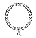
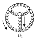
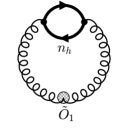
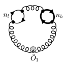
(e)	(f)	(g)	(h)

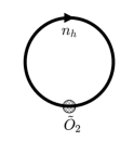
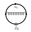
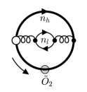
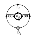
Figure 2: Sample diagrams contributing to $\zeta_{n}^{(m)}$ ($m\in\{0,2\}$) and $\zeta_{n3}$, for $n=1$ (a-d) and $n=2$ (e-h). The notation is the same as in Fig. 1; in addition, white circles denote flow-vertices, and lines with arrows next to them denote flow-lines (see Ref. [Artz:2019bpr] for details). Diagrams (a) and (b) only contribute to $\zeta_{1}^{(0)}$.

Therefore, the only coefficients that are not yet known through NNLO are

$$\begin{split}\zeta^{(2)}_{1},\,\zeta^{(2)}_{2},\,\zeta_{13}\,\text{ and }\zeta_{23}\,.\end{split}$$ (4.10)

According to Eq. (4.3), they require the calculation of derivatives w.r.t. $m_{\text{{B}}}$ in $\langle\tilde{O}_{1}(t)\rangle$ and $\langle\tilde{O}_{2}(t)\rangle$ up to three loops (see Fig. 2 for a set of associated diagrams). We achieved this using the setup described in Ref. [Artz:2019bpr], which employs qgraf[Nogueira:1991ex, Nogueira:2006pq] and q2e/exp[Harlander:1997zb, Seidensticker:1999bb] for the generation and subsequent categorization of the Feynman diagrams, FORM [Vermaseren:2000nd, Kuipers:2012rf] for the manipulation of the ensuing algebraic expressions, the color package[vanRitbergen:1998pn] of FORM for the calculation of the gauge group factors, and Kira$\oplus$FireFly[Maierhoefer:2017hyi, Maierhoefer:2018gpa, Klappert:2020nbg, Klappert:2019emp, Klappert:2020aqs] for the Feynman integral reduction using integration-by-parts identities and the Laporta algorithm[Tkachov:1981wb, Chetyrkin:1981qh, Laporta:2001dd] over finite fields[Kauers:2008zz, Kant:2013vta, vonManteuffel:2014ixa, Peraro:2016wsq]. For the evaluation of the master integrals, we adopt the method described in Ref. [Harlander:2016vzb], which performs sector decomposition [Binoth:2003ak] with the help of FIESTA [Smirnov:2013eza, Smirnov:2015mct] in order to extract the UV poles, along with a fully symmetric integration rule of order 13 for the numerical evaluation of their coefficients[Genz:1983malik], implemented with high precision arithmetics by using the MPFR library[mpfr:2007]. Some intermediate steps of the calculation are done within Mathematica[Mathematica].

Multiplying the result by $Z_{m}^{2}$ suffices to obtain the renormalized expressions for $\zeta_{n}^{(2)}$, and we find, setting $\mu=\mu_{t}$,

$$\zeta_{1}^{(2)}(t) =\frac{3n_{\text{A}}n_{\text{h}}}{8\pi^{2}t}T_{\text{R}}\,\bar{a}_{s}\left[1+\bar{a}_{s}\left(7.43789\,C_{\text{A}}+2\,C_{\text{F}}-\frac{10}{9}T_{\text{R}}n_{\text{f}}\right)\right]+{\cal O}(a_{s}^{3})\,,$$ (4.11a)

$$\zeta_{2}^{(2)}(t) =\frac{n_{\text{c}}n_{\text{h}}}{4\pi^{2}t}\bigg{[}1+\bar{a}_{s}C_{\text{F}}\left(\frac{7}{4}-\frac{3}{4}\ln 3\right)$$

$$\qquad+\bar{a}_{s}^{2}C_{\text{F}}\left(2.10889\,C_{\text{A}}+2.05158\,C_{\text{F}}-0.268909\,T_{\text{R}}n_{\text{f}}\right)\bigg{]}+{\cal O}(a_{s}^{3})\,,$$ (4.11b)

where again $\bar{a}_{s}=a_{s}(\mu_{t})$. Since quark loops appear in $\langle\tilde{O}_{1}(t)\rangle$ only at the two-loop level, $\zeta_{1}^{(2)}(t)$ starts at ${\cal O}(a_{s})$. In the case of $\zeta_{2}^{(2)}(t)$, the result for general $\mu$ can be obtained through multiplication by

$$\begin{split}\frac{m^{2}(\mu_{t})}{m^{2}(\mu)}=1+2\,a_{s}\,\gamma_{m,0}\,L_{\mu t}+2\,a_{s}^{2}\,L_{\mu t}\,\left[\gamma_{m,1}+\left(\frac{\beta_{0}\,\gamma_{m,0}}{2}+\gamma_{m,0}^{2}\right)\,L_{\mu t}\right]+{\cal O}(a_{s}^{3})\,,\end{split}$$ (4.12)

expressing $\bar{a}_{s}$ by $a_{s}$ through Eq. (4.8), and re-expanding in $a_{s}$. For $\zeta_{1}^{(2)}(t)$ one needs to multiply by Eq. (4.12), and in addition by $\bar{a}_{s}/a_{s}$.

$\zeta_{13}$ and $\zeta_{23}$ require the more sophisticated renormalization given in Eq. (4.6). It is important here to work consistently in $d$ space-time dimensions. Since $\vec{Z}_{3}$ contains a $1/\epsilon$ pole already at ${\cal O}(a_{s}^{0})$, we need to keep the ${\cal O}(\epsilon^{2})$ terms of $\zeta_{2\times 2}$ at NLO, and the ${\cal O}(\epsilon)$ terms at NNLO. They were not required in the calculation of Ref. [Harlander:2018zpi], so we recalculated $\zeta_{2\times 2}$, keeping these higher terms in $\epsilon$. Using the identity $n_{\text{A}}T_{\text{R}}=n_{\text{c}}C_{\text{F}}$[vanRitbergen:1998pn], our final result for $\vec{\zeta}_{3}$ reads:

$$\zeta_{13}(t) =\frac{n_{\text{h}}n_{\text{c}}C_{\text{F}}}{16\pi^{2}}a_{s}\bigg{\{}5-6\,\zeta(2)-6\,L_{\mu t}-6\,L_{\mu t}^{2}$$

$$\hskip 10.00002pt+a_{s}\,\bigg{[}-3.31445\,C_{\text{A}}-27.5707\,C_{\text{F}}-15.0886\,T_{\text{R}}n_{\text{h}}+19.5780\,T_{\text{R}}n_{\text{l}}$$

$$\hskip 20.00003pt+L_{\mu t}\,\bigg{(}-5.68293\,C_{\text{A}}-32.7594\,C_{\text{F}}-4.17386\,T_{\text{R}}n_{\text{h}}+19.8261\,T_{\text{R}}n_{\text{l}}\bigg{)}$$

$$\hskip 20.00003pt+L_{\mu t}^{2}\,\bigg{(}-\frac{433}{12}\,C_{\text{A}}-\frac{33}{2}\,C_{\text{F}}+\frac{26}{3}\,T_{\text{R}}n_{\text{f}}\bigg{)}$$

$$\hskip 20.00003pt+L_{\mu t}^{3}\,\bigg{(}-\frac{22}{3}\,C_{\text{A}}-6\,C_{\text{F}}+\frac{8}{3}\,T_{\text{R}}n_{\text{f}}\bigg{)}\bigg{]}\bigg{\}}+{\cal O}(a_{s}^{3})\,,$$ (4.13a)

$$\zeta_{23}(t) =\frac{n_{\text{c}}n_{\text{h}}}{2\pi^{2}}\bigg{\{}1+L_{\mu t}+a_{s}C_{\text{F}}\bigg{[}\frac{67}{16}+\frac{13}{2}\,\ln 2-\frac{15}{2}\,\ln 3-\frac{9}{4}\,\text{Li}_{2}(1/4)$$

$$\hskip 20.00003pt+\bigg{(}\frac{33}{8}-\ln 2-\frac{3}{4}\,\ln 3\bigg{)}\,L_{\mu t}+\frac{3}{2}\,L_{\mu t}^{2}\bigg{]}$$

$$\hskip 10.00002pt+a_{s}^{2}C_{\text{F}}\bigg{[}-0.710509\,C_{\text{A}}+6.97943\,C_{\text{F}}-6.43804\,T_{\text{R}}n_{\text{h}}-2.87689\,T_{\text{R}}n_{\text{l}}$$

$$\hskip 20.00003pt+L_{\mu t}\,\bigg{(}1.53754\,C_{\text{A}}+4.22899\,C_{\text{F}}-4.47865\,T_{\text{R}}n_{\text{h}}-1.47865\,T_{\text{R}}n_{\text{l}}\bigg{)}$$

$$\hskip 20.00003pt+L_{\mu t}^{2}\,\bigg{(}2.57807\,C_{\text{A}}+4.09934\,C_{\text{F}}-0.931798\,T_{\text{R}}n_{\text{f}}\bigg{)}$$

$$\hskip 20.00003pt+L_{\mu t}^{3}\,\bigg{(}\frac{11}{24}\,C_{\text{A}}+\frac{3}{2}\,C_{\text{F}}-\frac{1}{6}\,T_{\text{R}}n_{\text{f}}\bigg{)}\bigg{]}\bigg{\}}+{\cal O}(a_{s}^{3})\,.$$ (4.13b)

The logarithmic terms at ${\cal O}(a_{s}^{n})$ are determined by the RG equation derived in Sect. 5. Nevertheless, for the convenience of the reader, we provide the result for general $\mu$ in this case.

This, together with the results for $\zeta_{2\times 2}$ obtained in Refs. [Harlander:2018zpi] and explicitly given in Eq. (C.5), completes the result for the small-flow-time coefficients of the OPE up to dimension four of Eq. (3.18).

5 Flow-time evolution

In the final section of this paper we derive a general flow-time evolution equation for flowed operators. It resembles the RG equation for regular operators but with a “flowed anomalous dimension matrix”. While studies of the relation between the RG and the flow-time evolution have also been performed elsewhere in the literature (see, e.g., Refs. [Makino:2018rys, Carosso:2018rep, Abe:2018zdc, Carosso:2019qpb, Sonoda:2019ibh]), to our knowledge the treatment described here has not been discussed before.

Let us return to the small-flow-time expansion of the operators $\bar{O}$ defined in Eqs. (3.15), (3.17), employing a matrix rather than component-wise notation for the sake of clarity:

$$\begin{split}\bar{O}(t)=\zeta^{\text{{B}}}(t)O=\zeta(t)O^{\text{{R}}}\,.\end{split}$$ (5.1)

Since we work in the small-flow-time limit, the dependence of $\zeta(t)$ on $t$ can be only through $L_{\mu t}$, defined in Eq. (3.11). Taking the logarithmic derivative w.r.t. $t$ of Eq. (5.1), one thus obtains

$$\begin{split}t\partial_{t}\bar{O}(t)=(t\partial_{t}\zeta(t))O^{\text{{R}}}\,.\end{split}$$ (5.2)

Using Eq. (5.1) to eliminate the regular operators $O^{\text{{R}}}$, we find the flow-equation for flowed composite operators:

$$\begin{split}t\partial_{t}\bar{O}(t)=\gamma^{\text{f}}(t)\,\bar{O}(t)\,,\quad\mbox{where}\quad\gamma^{\text{f}}(t)\equiv(t\partial_{t}\zeta(t))\zeta^{-1}(t)\,.\end{split}$$ (5.3)

So far the discussion is general and holds for any flowed OPE. Specializing to our case of the QCD dimension-four operators, we can write the “flowed anomalous dimension” matrix as

$$\begin{split}\gamma^{\text{f}}=\left(\begin{matrix}\gamma^{\text{f}}_{2\times 2}&\vec{\gamma}^{\text{f}}_{3}\\ 0&0\end{matrix}\right)\,,\qquad\gamma^{\text{f}}_{2\times 2}(t)&=\left(t\partial_{t}\zeta_{2\times 2}(t)\right)\zeta^{-1}_{2\times 2}(t)\,,\\ \vec{\gamma}^{\text{f}}_{3}(t)&=-\gamma^{\text{f}}_{2\times 2}(t)\vec{\zeta}_{3}(t)+t\partial_{t}\vec{\zeta}_{3}(t)\,.\end{split}$$ (5.4)

Through ${\cal O}(a_{s}^{2})$, the result can be directly evaluated from Eqs. (C.5) and (4.13). A consistency check is obtained by noting that $\zeta(t)$ depends on $t$ only through $L_{\mu t}$:

$$\begin{split}t\partial_{t}\zeta(t)=\mu^{2}\frac{\partial}{\partial\mu^{2}}\zeta(t)=\mu^{2}\frac{\mathrm{d}}{\mathrm{d}\mu^{2}}\zeta(t)-a_{s}\beta\frac{\partial}{\partial a_{s}}\zeta(t)\,.\end{split}$$ (5.5)

On the other hand, we know that $a_{s}\tilde{O}_{1}(t)$ and $\tilde{O}_{2}(t)$ are RG invariant[Luscher:2010iy, Luscher:2011bx, Makino:2014taa] and therefore, with Eq. (3.15),

$$\begin{split}\left(\begin{matrix}0\\ 0\\ 4m^{4}\gamma_{m}\end{matrix}\right)&=\mu^{2}\frac{\mathrm{d}}{\mathrm{d}\mu^{2}}H^{-1}(a_{s})\tilde{O}(t)=\\ &=\mu^{2}\frac{\mathrm{d}}{\mathrm{d}\mu^{2}}H^{-1}(a_{s})\left(\zeta^{(0)}(t)\mathds{1}+\zeta^{(2)}(t)m^{2}\mathds{1}+\zeta(t)O^{\text{{R}}}\right)\,,\end{split}$$ (5.6)

where

$$\begin{split}H(x)=\left(\begin{matrix}H_{2\times 2}(x)&\vec{0}\\ \vec{0}^{\,T}&1\end{matrix}\right)\,,\quad\text{with}\quad H_{2\times 2}(x)=\left(\begin{matrix}(4\pi^{2}x)^{-1}&0\\ 0&1\end{matrix}\right)\,.\end{split}$$ (5.7)

Since operators of different mass dimensions do not mix under RG evolution and $\zeta_{3}^{(0,2)}(t)=0$, we can drop the first two terms in the brackets on the r.h.s. of Eq. (5.6). We thus arrive at

$$\begin{split}\mu^{2}\frac{\mathrm{d}}{\mathrm{d}\mu^{2}}\zeta(t)=\left(\begin{matrix}0&0&0\\ 0&0&0\\ 0&0&4\gamma_{m}\end{matrix}\right)-\left(\begin{matrix}\beta&0&0\\ 0&0&0\\ 0&0&0\end{matrix}\right)\zeta(t)-\zeta(t)\gamma^{O}\,,\end{split}$$ (5.8)

where $\gamma^{O}$ is the anomalous dimension of the operators $O^{\text{{R}}}$, defined through

$$\begin{split}\mu^{2}\frac{\mathrm{d}}{\mathrm{d}\mu^{2}}O^{\text{{R}}}=\gamma^{O}(a_{s})O^{\text{{R}}}\,.\end{split}$$ (5.9)

It can be written as

$$\begin{split}\gamma^{O}=\left(\mu^{2}\frac{\mathrm{d}}{\mathrm{d}\mu^{2}}Z\right)Z^{-1}=\left(\begin{matrix}\gamma^{O}_{2\times 2}&\vec{\gamma}^{\,O}_{3}\\[5.0pt] \vec{0}^{\,T}&4\gamma_{m}\end{matrix}\right)\,,\end{split}$$ (5.10)

with $Z$ from Eq. (2.10). Using the expressions of Sect. 2.1, one derives[Spiridonov:1984br, Spiridonov:1988md]

$$\begin{split}\gamma^{O}_{2\times 2}&=\left(\mu^{2}\frac{\mathrm{d}}{\mathrm{d}\mu^{2}}Z_{2\times 2}\right)Z^{-1}_{2\times 2}=\left(\begin{matrix}-\displaystyle a_{s}\frac{\partial}{\partial a_{s}}\beta&\displaystyle-2\,a_{s}\frac{\partial}{\partial a_{s}}\gamma_{m}\\[10.00002pt] 0&0\end{matrix}\right)\,,\\ \vec{\gamma}^{\,O}_{3}&=Z_{m}^{4}\left(\mu^{2}\frac{\mathrm{d}}{\mathrm{d}\mu^{2}}\vec{Z}_{3}-\gamma^{O}_{2\times 2}\vec{Z}_{3}\right)=\left(\begin{matrix}\displaystyle 4a_{s}\frac{\partial}{\partial a_{s}}\gamma_{0}\\[10.00002pt] 8\gamma_{0}\end{matrix}\right)\,.\end{split}$$ (5.11)

The QCD renormalization group functions $\beta$ and $\gamma_{m}$ are defined in Eqs. (A.2) and (A.4), respectively. Since they are of ${\cal O}(a_{s})$, the explicit $\mu$-dependence of $\zeta_{2\times 2}(t)$ can be derived through ${\cal O}(a_{s}^{3})$ from the results of Ref. [Harlander:2018zpi]. Thus, for $\gamma^{\text{f}}_{2\times 2}$, Eq. (5.5) is not just a consistency check, but a means to derive higher order terms. In our case, we can obtain the result through ${\cal O}(a_{s}^{3})$:

$$\gamma^{\text{f}}_{11} =a_{s}^{2}\,\bigg{[}\frac{3}{32}\,C_{\text{A}}^{2}+\frac{1}{8}\,C_{\text{A}}T_{\text{R}}n_{\text{f}}+\frac{7}{8}\,C_{\text{F}}T_{\text{R}}n_{\text{f}}\bigg{]}+a_{s}^{3}\,\bigg{[}-\frac{7}{48}\,C_{\text{A}}T_{\text{R}}^{2}n_{\text{f}}^{2}$$

$$\hskip 10.00002pt-\frac{35}{36}\,C_{\text{F}}T_{\text{R}}^{2}n_{\text{f}}^{2}+C_{\text{A}}C_{\text{F}}T_{\text{R}}n_{\text{f}}\,\bigg{(}\frac{11891}{2880}+\frac{27}{40}\,\ln 2-\frac{81}{160}\,\ln 3\bigg{)}$$

$$\hskip 10.00002pt+C_{\text{A}}^{2}T_{\text{R}}n_{\text{f}}\,\bigg{(}\frac{1687}{2880}+\frac{29}{40}\,\ln 2-\frac{9}{20}\,\ln 3\bigg{)}+C_{\text{A}}^{3}\,\bigg{(}\frac{6643}{11520}-\frac{319}{160}\,\ln 2+\frac{99}{80}\,\ln 3\bigg{)}$$

$$\hskip 10.00002pt+C_{\text{F}}^{2}T_{\text{R}}n_{\text{f}}\,\bigg{(}\frac{25}{64}+\frac{45}{8}\,\ln 2-\frac{111}{32}\,\ln 3+\frac{3}{4}\,\text{Li}_{2}(1/4)-\frac{3}{8}\,\zeta(2)\bigg{)}$$

$$\hskip 10.00002pt+\bigg{(}\frac{1}{6}\,C_{\text{A}}^{2}T_{\text{R}}n_{\text{f}}+\frac{11}{64}\,C_{\text{A}}^{3}+\frac{77}{48}\,C_{\text{A}}C_{\text{F}}T_{\text{R}}n_{\text{f}}-\frac{1}{12}\,C_{\text{A}}T_{\text{R}}^{2}n_{\text{f}}^{2}-\frac{7}{12}\,C_{\text{F}}T_{\text{R}}^{2}n_{\text{f}}^{2}\bigg{)}\,L_{\mu t}\bigg{]}$$

$$\hskip 10.00002pt+{\cal O}(a_{s}^{4})\,,$$ (5.12a)

$$\gamma^{\text{f}}_{12} =-\frac{3}{2}\,a_{s}\,C_{\text{F}}+a_{s}^{2}\,\Bigg{\{}-\frac{367}{48}\,C_{\text{A}}C_{\text{F}}+\frac{5}{3}\,C_{\text{F}}T_{\text{R}}n_{\text{f}}+C_{\text{F}}^{2}\,\bigg{[}-\frac{3}{16}-\frac{3}{2}\,\ln 2-\frac{9}{8}\,\ln 3\bigg{]}$$

$$\hskip 10.00002pt+\bigg{[}-\frac{11}{4}\,C_{\text{A}}C_{\text{F}}+C_{\text{F}}T_{\text{R}}n_{\text{f}}\bigg{]}\,L_{\mu t}\Bigg{\}}$$

$$+a_{s}^{3}\,\Bigg{\{}C_{\text{F}}^{2}C_{\text{A}}\,\bigg{[}-\frac{391}{768}-\frac{431}{24}\,\ln 2+\frac{3}{8}\,\ln^{2}2+\frac{11}{64}\,\ln 3+\frac{9}{8}\,\text{Li}_{2}(1/4)-\frac{33}{64}\,\zeta(2)\bigg{]}$$

$$\hskip 10.00002pt+C_{\text{F}}T_{\text{R}}^{2}n_{\text{f}}^{2}\,\bigg{[}-\frac{25}{18}-\frac{1}{2}\,\zeta(2)\bigg{]}+C_{\text{F}}^{3}\,\bigg{[}-\frac{1401}{256}+\frac{339}{16}\,\ln 2-\frac{9}{8}\,\ln^{2}2$$

$$\hskip 20.00003pt-\frac{657}{64}\,\ln 3-\frac{9}{4}\,\ln 2\,\ln 3-\frac{27}{32}\,\ln^{2}3+\frac{153}{32}\,\text{Li}_{2}(1/4)+\frac{39}{64}\,\zeta(2)\bigg{]}$$

$$\hskip 10.00002pt+C_{\text{A}}^{2}C_{\text{F}}\,\bigg{[}-\frac{5291}{144}-\frac{2311}{24}\,\ln 2+\frac{4641}{64}\,\ln 3+\frac{11}{32}\,\text{Li}_{2}(1/4)+\frac{11}{8}\,\zeta(2)\bigg{]}$$

$$\hskip 10.00002pt+C_{\text{F}}^{2}T_{\text{R}}n_{\text{f}}\,\bigg{[}\frac{8827}{960}-\frac{2089}{120}\,\ln 2+\frac{847}{80}\,\ln 3+\frac{3}{8}\,\text{Li}_{2}(1/4)-\frac{3}{16}\,\zeta(2)-\frac{9}{2}\,\zeta(3)\bigg{]}$$

$$\hskip 10.00002pt+C_{\text{A}}C_{\text{F}}T_{\text{R}}n_{\text{f}}\,\bigg{[}\frac{5861}{360}+\frac{4273}{120}\,\ln 2-\frac{2139}{80}\,\ln 3-\frac{1}{8}\,\text{Li}_{2}(1/4)+\frac{7}{8}\,\zeta(2)+\frac{9}{2}\,\zeta(3)\bigg{]}$$

$$\hskip 20.00003pt+\frac{3}{32}\,C_{\text{F}}\,c_{\chi}^{(2)}+\bigg{[}-\frac{4445}{192}\,C_{\text{A}}^{2}C_{\text{F}}+\frac{647}{48}\,C_{\text{A}}C_{\text{F}}T_{\text{R}}n_{\text{f}}-\frac{5}{3}\,C_{\text{F}}T_{\text{R}}^{2}n_{\text{f}}^{2}$$

$$\hskip 20.00003pt+C_{\text{F}}^{2}C_{\text{A}}\,\bigg{(}-\frac{33}{64}-\frac{33}{8}\,\ln 2-\frac{99}{32}\,\ln 3\bigg{)}+C_{\text{F}}^{2}T_{\text{R}}n_{\text{f}}\,\bigg{(}\frac{15}{16}+\frac{3}{2}\,\ln 2+\frac{9}{8}\,\ln 3\bigg{)}\bigg{]}\,L_{\mu t}$$

$$\hskip 10.00002pt+\bigg{[}-\frac{121}{32}\,C_{\text{A}}^{2}C_{\text{F}}+\frac{11}{4}\,C_{\text{A}}C_{\text{F}}T_{\text{R}}n_{\text{f}}-\frac{1}{2}\,C_{\text{F}}T_{\text{R}}^{2}n_{\text{f}}^{2}\bigg{]}\,L_{\mu t}^{2}\Bigg{\}}+{\cal O}(a_{s}^{4})\,,$$ (5.12b)

$$\gamma^{\text{f}}_{21} =a_{s}^{3}\,\bigg{[}C_{\text{A}}^{2}T_{\text{R}}n_{\text{f}}\,\bigg{(}\frac{599}{5760}+\frac{33}{80}\,\ln 2-\frac{99}{320}\,\ln 3\bigg{)}+C_{\text{A}}T_{\text{R}}^{2}n_{\text{f}}^{2}\,\bigg{(}\frac{41}{1440}$$

$$\hskip 20.00003pt-\frac{3}{20}\,\ln 2+\frac{9}{80}\,\ln 3\bigg{)}+C_{\text{A}}C_{\text{F}}T_{\text{R}}n_{\text{f}}\,\bigg{(}\frac{209}{1152}+\frac{55}{16}\,\ln 2-\frac{407}{192}\,\ln 3$$

$$\hskip 20.00003pt+\frac{11}{24}\,\text{Li}_{2}(1/4)-\frac{11}{48}\,\zeta(2)\bigg{)}+C_{\text{F}}T_{\text{R}}^{2}n_{\text{f}}^{2}\,\bigg{(}\frac{43}{144}-\frac{5}{4}\,\ln 2+\frac{37}{48}\,\ln 3$$

$$\hskip 20.00003pt-\frac{1}{6}\,\text{Li}_{2}(1/4)+\frac{1}{12}\,\zeta(2)\bigg{)}\bigg{]}+{\cal O}(a_{s}^{4})\,,$$ (5.12c)

$$\gamma^{\text{f}}_{22} =a_{s}^{2}\,\Bigg{[}C_{\text{A}}C_{\text{F}}\,\bigg{(}\frac{11}{96}-\frac{11}{12}\,\ln 2-\frac{11}{16}\,\ln 3\bigg{)}+C_{\text{F}}T_{\text{R}}n_{\text{f}}\,\bigg{(}-\frac{2}{3}+\frac{1}{3}\,\ln 2$$

$$\hskip 20.00003pt+\frac{1}{4}\,\ln 3\bigg{)}\Bigg{]}+a_{s}^{3}\,\Bigg{\{}C_{\text{A}}C_{\text{F}}T_{\text{R}}n_{\text{f}}\,\bigg{[}\frac{2521}{960}-\frac{1709}{90}\,\ln 2-\frac{1}{6}\,\ln^{2}2$$

$$\hskip 20.00003pt+\frac{1537}{160}\,\ln 3-\frac{1}{24}\,\text{Li}_{2}(1/4)\bigg{]}+C_{\text{A}}^{2}C_{\text{F}}\,\bigg{[}-\frac{7397}{2304}-\frac{213}{16}\,\ln 2+\frac{11}{24}\,\ln^{2}2$$

$$\hskip 20.00003pt+\frac{107}{16}\,\ln 3+\frac{11}{8}\,\text{Li}_{2}(1/4)-\frac{121}{192}\,\zeta(2)\bigg{]}+C_{\text{F}}T_{\text{R}}^{2}n_{\text{f}}^{2}\,\bigg{[}-\frac{749}{720}+\frac{763}{90}\,\ln 2$$

$$\hskip 20.00003pt-\frac{83}{20}\,\ln 3-\frac{1}{6}\,\text{Li}_{2}(1/4)+\frac{1}{12}\,\zeta(2)\bigg{]}+C_{\text{F}}^{2}T_{\text{R}}n_{\text{f}}\,\bigg{[}-\frac{139}{192}-\frac{119}{8}\,\ln 2$$

$$\hskip 20.00003pt+\frac{1}{6}\,\ln^{2}2+\frac{261}{32}\,\ln 3+\frac{1}{2}\,\ln 2\,\ln 3+\frac{3}{16}\,\ln^{2}3-\frac{23}{8}\,\text{Li}_{2}(1/4)+\frac{5}{48}\,\zeta(2)\bigg{]}$$

$$\hskip 10.00002pt+C_{\text{F}}^{2}C_{\text{A}}\,\bigg{[}\frac{253}{384}+\frac{209}{8}\,\ln 2-\frac{11}{24}\,\ln^{2}2-\frac{99}{8}\,\ln 3-\frac{11}{8}\,\ln 2\,\ln 3-\frac{33}{64}\,\ln^{2}3$$

$$\hskip 20.00003pt+\frac{187}{32}\,\text{Li}_{2}(1/4)+\frac{143}{192}\,\zeta(2)\bigg{]}+\bigg{(}\frac{11}{96}\,C_{\text{A}}-\frac{1}{24}\,T_{\text{R}}n_{\text{f}}\bigg{)}\,c_{\chi}^{(2)}$$

$$\hskip 20.00003pt+\bigg{[}C_{\text{A}}^{2}C_{\text{F}}\,\bigg{(}\frac{121}{576}-\frac{121}{72}\,\ln 2-\frac{121}{96}\,\ln 3\bigg{)}+C_{\text{F}}T_{\text{R}}^{2}n_{\text{f}}^{2}\,\bigg{(}\frac{4}{9}-\frac{2}{9}\,\ln 2-\frac{1}{6}\,\ln 3\bigg{)}$$

$$\hskip 20.00003pt+C_{\text{A}}C_{\text{F}}T_{\text{R}}n_{\text{f}}\,\bigg{(}-\frac{187}{144}+\frac{11}{9}\,\ln 2+\frac{11}{12}\,\ln 3\bigg{)}\bigg{]}\,L_{\mu t}\Bigg{\}}+{\cal O}(a_{s}^{4})\,.$$ (5.12d)

We verified that this agrees through ${\cal O}(a_{s}^{2})$ with the result which is obtained by directly inserting Eq. (C.5) into Eq. (5.4). Due to the factor of $1/g^{2}$ in $\tilde{O}_{1}$ (see Eq. (3.1)), $\gamma^{\text{f}}_{2\times 2}$ is not RG invariant, while $H^{-1}_{2\times 2}\gamma^{\text{f}}_{2\times 2}H_{2\times 2}$ is. It may be useful to note that, by subtracting the VEVs off of $\tilde{O}_{1}$ and $\tilde{O}_{2}$,

$$\begin{split}\tilde{O}_{1,\text{sub}}(t,x)&=\tilde{O}_{1}(t,x)-\langle\tilde{O}_{1}(t,x)\rangle\,,\\ \tilde{O}_{2,\text{sub}}(t,x)&=\tilde{O}_{2}(t,x)-\langle\tilde{O}_{2}(t,x)\rangle\,,\end{split}$$ (5.13)

the resulting operators do not mix with $\tilde{O}_{3}$ under $t$-evolution. Rather, their logarithmic $t$-evolution is fully governed by $\gamma^{\text{f}}_{2\times 2}$ and thus known through ${\cal O}(a_{s}^{3})$.

Eq. (5.8) does not analogously allow one to derive the ${\cal O}(a_{s}^{3})$ terms of $\vec{\gamma}^{\text{f}}_{3}$, because it involves $\gamma_{0}$ which, in contrast to $\beta$ and $\gamma_{m}$, starts at ${\cal O}(a_{s}^{0})$ rather than ${\cal O}(a_{s})$, see Eq. (A.7). Therefore, we can only give the result through ${\cal O}(a_{s}^{2})$ for $\vec{\gamma}^{\text{f}}_{3}$:

$$\gamma_{13}^{\text{f}} =\frac{3n_{\text{c}}n_{\text{h}}}{8\pi^{2}}a_{s}C_{\text{F}}\bigg{\{}1+a_{s}\bigg{[}9.24729\,C_{\text{A}}-2.47340\,C_{\text{F}}$$

$$\hskip 10.00002pt-2.91787\,T_{\text{R}}n_{\text{h}}+1.08213\,T_{\text{R}}n_{\text{l}}+L_{\mu t}\,\bigg{(}\frac{11}{6}\,C_{\text{A}}+3\,C_{\text{F}}-\frac{2}{3}\,T_{\text{R}}n_{\text{f}}\bigg{)}\bigg{]}\bigg{\}}\,,$$ (5.14a)

$$\gamma_{23}^{\text{f}} =\frac{n_{\text{c}}n_{\text{h}}}{2\pi^{2}}\bigg{\{}1+a_{s}C_{\text{F}}\left[\frac{33}{8}-\ln 2-\frac{3}{4}\ln 3+3\,L_{\mu t}\right]+a_{s}^{2}C_{\text{F}}\bigg{[}2.81363\,C_{\text{A}}+4.22899\,C_{\text{F}}$$

$$\hskip 10.00002pt-4.31769\,T_{\text{R}}n_{\text{h}}-1.31769\,T_{\text{R}}n_{\text{l}}+L_{\mu t}\,\bigg{(}6.43224\,C_{\text{A}}+8.19868\,C_{\text{F}}-1.70263\,T_{\text{R}}n_{\text{f}}\bigg{)}$$

$$\hskip 10.00002pt+L_{\mu t}^{2}\,\bigg{(}\frac{11}{8}\,C_{\text{A}}+\frac{9}{2}\,C_{\text{F}}-\frac{1}{2}\,T_{\text{R}}n_{\text{f}}\bigg{)}\bigg{]}\bigg{\}}\,.$$ (5.14b)

We checked, of course, that Eq. (5.8) is consistent with the results for $\zeta_{13}$ and $\zeta_{23}$ of Eq. (4.13).

6 Conclusions

We presented the flowed OPE for general current correlators and its matching to regular QCD through NNLO in the strong coupling $\alpha_{s}$ and through mass dimension four by using the small-flow-time expansion. Our calculation is based on the renormalization procedure for the regular QCD dimension-four operators worked out in Ref. [Spiridonov:1984br, Spiridonov:1988md], the mixing matrix between flowed and regular operators derived in Ref. [Harlander:2018zpi], the method of projectors [Gorishnii:1983su], and the tools and results for perturbative calculations in the GFF presented in Ref. [Artz:2019bpr].

Overall, our results allow to combine the known perturbative results for the regular QCD current correlators from the literature to gradient-flow lattice calculations. This lays out the path for an alternative determination of hadronic contributions to observables such as the anomalous magnetic moment of the muon. In addition, we derived a general logarithmic flow-time evolution equation for flowed operators and presented its explicit form for the dimension-four operators considered in this paper.

Our methods are sufficiently general to be applied to similar problems at higher orders in perturbation theory, such as CP violating operators [Rizik:2020naq] relevant for the electric dipole moment of the neutron, or four-quark operators occurring in flavor physics[Suzuki:2020zue].

Acknowledgments.

We would like to thank A. Hoang for confirmative comments on the validity of the approach pursued in this paper, and Y. Kluth for helpful comments and clarifications. RVH would like to thank K. Chetyrkin for past initiation and collaboration on the material of Sect. 2.

This work was supported by Deutsche Forschungsgemeinschaft (DFG) through project HA 2990/9-1, and by the U.S. Department of Energy under award No. DE-SC0008347. This document was prepared using the resources of the Fermi National Accelerator Laboratory (Fermilab), a U.S. Department of Energy, Office of Science, HEP User Facility. Fermilab is managed by Fermi Research Alliance, LLC (FRA), acting under Contract No. DE-AC02-07CH11359.

Appendix A Renormalization group functions

The $d$-dimensional beta function is defined as

$$\begin{split}\mu^{2}\frac{\mathrm{d}}{\mathrm{d}\mu^{2}}a_{s}(\mu)=a_{s}(\mu)\beta_{\epsilon}(a_{s}(\mu))\,,\end{split}$$ (A.1)

where $a_{s}\equiv\alpha_{s}/\pi\equiv g^{2}/(4\pi^{2})$. The renormalized coupling $g=g(\mu)$ is related to the bare one through $g_{\text{{B}}}=\hat{\mu}^{\epsilon}\,Z_{s}^{1/2}\,g$, where $Z_{s}$ is the $\overline{\mbox{{MS}}}$ renormalization constant. From this follow the relations

$$\begin{split}\beta_{\epsilon}(a_{s})&=-\epsilon\left(1+a_{s}\frac{\partial}{\partial a_{s}}\ln Z_{s}(a_{s})\right)^{-1}=-\epsilon+\beta(a_{s})\equiv-\epsilon-\sum_{n\geq 0}a_{s}^{n+1}\beta_{n}\,,\\ Z_{s}(a_{s})&=1-\frac{a_{s}}{\epsilon}\beta_{0}+a_{s}^{2}\left(\frac{1}{\epsilon^{2}}\beta_{0}^{2}-\frac{1}{2\epsilon}\beta_{1}\right)+{\cal O}(a_{s}^{3})\,.\end{split}$$ (A.2)

Through Sect. 5, we only need the first two perturbative coefficients, while $\beta_{2}$ is required in order to derive the ${\cal O}(a_{s}^{3})$ terms of $\gamma^{\text{f}}$ in Eq. (5.12):

$$\begin{split}\beta_{0}&=\frac{1}{4}\left(\frac{11}{3}C_{\text{A}}-\frac{4}{3}T_{\text{R}}n_{\text{f}}\right)\,,\qquad\beta_{1}=\frac{1}{16}\left(\frac{34}{3}C_{\text{A}}^{2}-4C_{\text{F}}T_{\text{R}}n_{\text{f}}-\frac{20}{3}C_{\text{A}}T_{\text{R}}n_{\text{f}}\right)\,,\\ \beta_{2}&=\frac{1}{64}\bigg{(}\frac{2857}{54}C_{\text{A}}^{3}+2C_{\text{F}}^{2}T_{\text{R}}n_{\text{f}}-\frac{205}{9}C_{\text{F}}C_{\text{A}}T_{\text{R}}n_{\text{f}}-\frac{1415}{27}C_{\text{A}}^{2}T_{\text{R}}n_{\text{f}}\\ &\qquad+\frac{44}{9}C_{\text{F}}T_{\text{R}}^{2}n_{\text{f}}^{2}+\frac{158}{27}C_{\text{A}}T_{\text{R}}^{2}n_{\text{f}}^{2}\bigg{)}\,.\end{split}$$ (A.3)

The anomalous dimension of the quark mass is defined through

$$\begin{split}\gamma_{m}(a_{s})&=-a_{s}\beta_{\epsilon}(a_{s})\frac{\partial}{\partial a_{s}}\ln Z_{m}(a_{s})\equiv-\sum_{n\geq 0}a_{s}^{n+1}\gamma_{m,n}\,,\end{split}$$ (A.4)

with the first three perturbative coefficients given by

$$\begin{split}\gamma_{m,0}&=\frac{3}{4}C_{\text{F}}\,,\qquad\gamma_{m,1}=\frac{3}{32}C_{\text{F}}^{2}+\frac{97}{96}C_{\text{A}}C_{\text{F}}-\frac{5}{24}C_{\text{F}}T_{\text{R}}n_{\text{f}}\,,\\ \gamma_{m,2}&=\frac{1}{64}\left[\frac{129}{2}C_{\text{F}}^{3}-\frac{129}{4}C_{\text{F}}^{2}C_{\text{A}}+\frac{11413}{108}C_{\text{F}}C_{\text{A}}^{2}\right.\\ &\left.+C_{\text{F}}^{2}T_{\text{R}}n_{\text{f}}(-46+48\zeta(3))+C_{\text{F}}C_{\text{A}}T_{\text{R}}n_{\text{f}}\left(-\frac{556}{27}-48\zeta(3)\right)-\frac{140}{27}C_{\text{F}}T_{\text{R}}^{2}n_{\text{f}}^{2}\right]\,.\end{split}$$ (A.5)

It determines the $\overline{\mbox{{MS}}}$ renormalized mass $m$ through

$$\begin{split}m_{\text{{B}}}=Z_{m}\,m\,,\qquad Z_{m}=1-\frac{a_{s}}{\epsilon}\gamma_{m,0}+a_{s}^{2}\left[\frac{\gamma_{m,0}}{2\epsilon^{2}}\left(\gamma_{m,0}+\beta_{0}\right)-\frac{1}{2\epsilon}\gamma_{m,1}\right]+{\cal O}(a_{s}^{3})\,.\end{split}$$ (A.6)

Similarly to $\beta_{\epsilon}$, the third coefficient $\gamma_{m,2}$ is needed only in Sect. 5.

The renormalization constant of the vacuum energy $Z_{0}$ is related to the corresponding anomalous dimension $\gamma_{0}$ through

$$\begin{split}\gamma_{0}(a_{s})&=\left[4\gamma_{m}(a_{s})-\epsilon\right]Z_{0}(a_{s})+\beta_{\epsilon}(a_{s})a_{s}\frac{\partial}{\partial a_{s}}Z_{0}(a_{s})\equiv-\frac{n_{\text{c}}n_{\text{h}}}{(4\pi)^{2}}\sum_{n\geq 0}a_{s}^{n}\gamma_{0,n}\,,\end{split}$$ (A.7)

which leads to

$$\begin{split}Z_{0}(a_{s})&=\frac{n_{\text{c}}n_{\text{h}}}{(4\pi)^{2}\epsilon}\bigg{\{}1+a_{s}\left(\frac{\gamma_{0,1}}{2}-\frac{2\gamma_{m,0}}{\epsilon}\right)+a_{s}^{2}\Big{[}\frac{2}{3\epsilon^{2}}\,\left(\beta_{0}\,\gamma_{m,0}+4\,\gamma_{m,0}^{2}\right)\\ &\qquad-\frac{1}{6\epsilon}\left(\beta_{0}\,\gamma_{0,1}+4\,\gamma_{0,1}\gamma_{m,0}+8\,\gamma_{m,1}\right)+\frac{1}{3}\gamma_{0,2}\Big{]}\bigg{\}}+{\cal O}(a_{s}^{3})\,.\end{split}$$ (A.8)

The first three perturbative coefficients are given by [Spiridonov:1988md, Chetyrkin:1994ex]

$$\begin{split}\gamma_{0,0}&=1\,,\qquad\gamma_{0,1}=C_{\text{F}}\,,\\ \gamma_{0,2}&=-C_{\text{F}}^{2}\,\left(\frac{131}{32}-3\,\zeta(3)\right)-C_{\text{F}}C_{\text{A}}\left(-\frac{109}{32}+\frac{3}{2}\,\zeta(3)\right)-C_{\text{F}}T_{\text{R}}\left(\frac{5}{8}n_{\text{f}}+3n_{\text{h}}\right)\,.\end{split}$$ (A.9)

Appendix B Perturbative coefficient functions

This appendix cites the results for the coefficient functions $C_{n}$ of the regular dimension-four operators appearing in the OPE of the current correlators defined in Eq. (2.2). We consider scalar, pseudo-scalar, vector- and axial-vector currents, both diagonal and non-diagonal, i.e. the currents assume the form

$$\begin{split}j(x)&=\bar{\psi}_{k}(x)\Gamma\psi_{l}(x)\,,\qquad\Gamma\in\{1,i\gamma_{5},\gamma^{\mu},\gamma^{\mu}\gamma_{5}\}\,,\\ k,l&\in N\cup M\,,\quad M=\{1,\ldots,n_{\text{h}}\}\,,\quad N=\{n_{\text{h}}+1,\ldots,n_{\text{f}}\}\,.\end{split}$$ (B.1)

This means that $\psi_{k}$ and $\psi_{l}$ can be either both massive with mass $m$ ($k,l\in M$), or both massless ($k,l\in N$), or one of them is massless, the other massive (e.g. $k\in M$, $l\in N$). While $C_{1}$ is independent of $k$ and $l$, the coefficient $C_{2}$ of the quark operator takes the form

$$\begin{split}C_{2}=C_{2,N}+\frac{1}{n_{\text{h}}}\left(\delta_{kM}+\delta_{lM}\right)\left(C_{2,M}+C_{2,\text{nd}}\right)\,,\end{split}$$ (B.2)

where $\delta_{kM}=1$ for $k\in M$, and 0 otherwise. Also the results for $C_{3}$ depend on whether the quarks $k$ and $l$ are massive or not. This dependence will be indicated explicitly below, using the $\delta_{kM}$ symbol defined above.

For convenience, we introduce the short-hand notation

$$\begin{split}l_{\mu Q}\equiv\ln\frac{Q^{2}}{\mu^{2}}\,,\end{split}$$ (B.3)

and the dimensionless quantities

$$\hat{C}_{1}=Q^{4}\,C_{1}\,,\qquad\hat{C}_{2}=-2\,Q^{4}\,C_{2}\,,\qquad\hat{C}_{3}=Q^{4}\,C_{3}\,.$$ (B.4)

The extra factor $(-2)$ between $C_{2}$ and $\hat{C}_{2}$ arises from using $O_{2}^{\prime}$ in Ref. [Harlander:diss] rather than $O_{2}$ from Eq. (2.5). For the sake of brevity, we insert the SU(3) color factors.

B.1 Vector and axial-vector currents

In this case, the current correlator can be decomposed into a transversal and a longitudinal part, each associated with a set of coefficient functions:

$$\int\mathrm{d}^{4}xe^{iqx}j^{v/a}_{\mu}(x)j^{v/a}_{\nu}(0)\stackrel{{\scriptstyle Q^{2}\to\infty}}{{\longrightarrow}}\sum_{n}\left((g_{\mu\nu}Q^{2}-Q_{\mu}Q_{\nu})C_{n}^{v/a,{\rm T}}-Q_{\mu}Q_{\nu}C_{n}^{v/a,{\rm L}}\right)O^{\text{{R}}}_{n}\,.$$ (B.5)

The upper sign refers to the vector, the lower sign to the axial-vector case. The results have been taken from Ref. [Harlander:diss]:

$$\hat{C}^{v/a,{\rm T}}_{1}=\frac{1}{12}\,a_{s}+\frac{7}{72}\,a_{s}^{2}\,,$$ (B.6a)

$$\hat{C}^{v/a,{\rm T}}_{2,N}=a_{s}^{2}\left(-1+\frac{1}{3}\,l_{\mu Q}+\frac{4}{3}\,\zeta(3)\right)\,,$$ (B.6b)

$$\hat{C}^{v/a,{\rm T}}_{2,M}=-a_{s}+a_{s}^{2}\,\bigg{[}-\frac{29}{6}+\frac{1}{6}\,n_{\text{f}}+l_{\mu Q}\,\bigg{(}-\frac{11}{4}+\frac{1}{6}\,n_{\text{f}}\bigg{)}\bigg{]}\,,$$ (B.6c)

$$\hat{C}^{v/a,{\rm T}}_{2,\text{nd}}=\pm\left(1+{4\over 3}\,a_{s}+a_{s}^{2}\,\bigg{[}{191\over 18}-{7\over 27}\,n_{\text{f}}+l_{\mu Q}\,\bigg{(}{11\over 3}-{2\over 9}\,n_{\text{f}}\bigg{)}\bigg{]}\right)\,,$$ (B.6d)

$$\hat{C}_{1}^{v/a,{\rm L}}=0\,,\qquad\hat{C}_{2,N}^{v/a,{\rm L}}=0\,,\qquad\hat{C}_{2,M}^{v/a,{\rm L}}=1\,,\qquad\hat{C}_{2,\text{nd}}^{v/a,{\rm L}}=\mp 1\,,$$ (B.6e)

$$\hat{C}^{v/a,{\rm T}}_{3}=\frac{3}{16\pi^{2}}\,\bigg{\{}\delta_{kM}\delta_{lM}\,\Bigg{[}a_{s}\,\bigg{(}\frac{152}{9}-\frac{32}{3}\,\zeta(3)\bigg{)}$$

$$\mbox{\hskip 20.00003pt}+a_{s}^{2}\,\bigg{[}\frac{1295}{9}-\frac{524}{3}\,\zeta(3)+120\,\zeta(5)+n_{\text{f}}\,\bigg{(}-\frac{362}{81}+\frac{8}{27}\,\zeta(3)\bigg{)}$$

$$\mbox{\hskip 30.00005pt}+l_{\mu Q}\,\bigg{(}114-72\,\zeta(3)+n_{\text{f}}\,\left(-\frac{76}{27}+\frac{16}{9}\,\zeta(3)\right)\bigg{)}\bigg{]}\Bigg{]}$$

$$\mbox{\hskip 10.00002pt}\pm 2\delta_{kM}\delta_{lM}\,\Bigg{[}-4\,l_{\mu Q}+a_{s}\,\bigg{(}-\frac{56}{3}+16\,\zeta(3)-\frac{32}{3}\,l_{\mu Q}-8\,l_{\mu Q}^{2}\bigg{)}$$

$$\mbox{\hskip 20.00003pt}+a_{s}^{2}\,\bigg{[}-\frac{18967}{108}+\frac{4588}{27}\,\zeta(3)+\frac{4}{3}\,\zeta(4)-\frac{280}{27}\,\zeta(5)+n_{\text{f}}\,\bigg{(}\frac{337}{54}-\frac{40}{9}\,\zeta(3)\bigg{)}$$

$$\mbox{\hskip 30.00005pt}+l_{\mu Q}\,\bigg{(}-\frac{3617}{18}+\frac{332}{3}\,\zeta(3)+n_{\text{f}}\,\left(\frac{157}{27}-\frac{8}{3}\,\zeta(3)\right)\bigg{)}$$

$$\mbox{\hskip 30.00005pt}+l_{\mu Q}^{2}\,\bigg{(}-77+\frac{22}{9}\,n_{\text{f}}\bigg{)}+l_{\mu Q}^{3}\,\bigg{(}-18+\frac{4}{9}\,n_{\text{f}}\bigg{)}\bigg{]}\Bigg{]}$$

$$\mbox{\hskip 10.00002pt}+(\delta_{kM}+\delta_{lM})\,\Bigg{[}-2+a_{s}\,\bigg{(}-4-4\,l_{\mu Q}\bigg{)}$$

$$\mbox{\hskip 20.00003pt}+a_{s}^{2}\,\bigg{[}-\frac{776}{27}+\frac{2996}{27}\,\zeta(3)-\frac{3440}{27}\,\zeta(5)+n_{\text{f}}\,\bigg{(}\frac{23}{27}-\frac{4}{9}\,\zeta(3)\bigg{)}$$

$$\mbox{\hskip 30.00005pt}+l_{\mu Q}\,\bigg{(}-36+\frac{10}{9}\,n_{\text{f}}\bigg{)}-8\,l_{\mu Q}^{2}\bigg{]}\Bigg{]}$$

$$\mbox{\hskip 10.00002pt}+n_{\text{h}}\,a_{s}^{2}\,\Bigg{[}-\frac{80}{9}+\frac{16}{3}\,\zeta(3)+l_{\mu Q}\,\bigg{(}\frac{40}{9}-\frac{16}{3}\,\zeta(3)\bigg{)}-\frac{2}{3}\,l_{\mu Q}^{2}\Bigg{]}$$

$$\mbox{\hskip 10.00002pt}+n_{\text{h}}\,a_{s}^{2}\,\Bigg{[}(\delta_{kM}+\delta_{lM})\,\bigg{(}\frac{100}{9}-\frac{16}{3}\,\zeta(3)\bigg{)}$$

$$\mbox{\hskip 10.00002pt}\pm\delta_{kM}\delta_{lM}\,\bigg{(}-\frac{64}{9}+16\,l_{\mu Q}+\frac{32}{3}\,\zeta(3)\bigg{)}\Bigg{]}\bigg{\}}\,,$$ (B.6f)

$$\hat{C}_{3}^{v/a,{\rm L}}=\frac{3}{16\pi^{2}}\,\bigg{\{}\delta_{kM}\delta_{lM}\,\Bigg{[}8+a_{s}\,\bigg{(}\frac{152}{3}+32\,l_{\mu Q}\bigg{)}$$

$$\mbox{\hskip 20.00003pt}+a_{s}^{2}\,\bigg{[}\frac{7306}{9}-\frac{1292}{9}\,\zeta(3)-\frac{640}{9}\,\zeta(5)+n_{\text{f}}\bigg{(}-\frac{212}{9}+\frac{8}{3}\,\zeta(3)\bigg{)}$$

$$\mbox{\hskip 30.00005pt}+l_{\mu Q}\,\bigg{(}\frac{1430}{3}-\frac{116}{9}\,n_{\text{f}}\bigg{)}+l_{\mu Q}^{2}\,\bigg{(}108-\frac{8}{3}\,n_{\text{f}}\bigg{)}\bigg{]}\Bigg{]}$$

$$\mbox{\hskip 10.00002pt}\pm 2\delta_{kM}\delta_{lM}\,\Bigg{[}4\,l_{\mu Q}+a_{s}\,\bigg{(}8-16\,\zeta(3)+\frac{16}{3}\,l_{\mu Q}+8\,l_{\mu Q}^{2}\bigg{)}$$

$$\mbox{\hskip 20.00003pt}+a_{s}^{2}\,\bigg{[}-\frac{6713}{108}-\frac{464}{3}\,\zeta(3)-\frac{4}{3}\,\zeta(4)+\frac{940}{9}\,\zeta(5)+n_{\text{f}}\bigg{(}\frac{31}{54}+\frac{8}{9}\,\zeta(3)\bigg{)}$$

$$\mbox{\hskip 30.00005pt}+l_{\mu Q}\,\bigg{(}\frac{1429}{18}-\frac{332}{3}\,\zeta(3)+n_{\text{f}}\left(-3+\frac{8}{3}\,\zeta(3)\right)\bigg{)}+l_{\mu Q}^{2}\,\bigg{(}\frac{155}{3}-\frac{14}{9}\,n_{\text{f}}\bigg{)}$$

$$\mbox{\hskip 30.00005pt}+l_{\mu Q}^{3}\,\bigg{(}18-\frac{4}{9}\,n_{\text{f}}\bigg{)}\bigg{]}\Bigg{]}$$

$$\mbox{\hskip 10.00002pt}+(\delta_{kM}+\delta_{lM})\Bigg{[}-4-4\,l_{\mu Q}+a_{s}\,\bigg{(}-\frac{100}{3}+16\,\zeta(3)-\frac{64}{3}\,l_{\mu Q}-8\,l_{\mu Q}^{2}\bigg{)}$$

$$\mbox{\hskip 20.00003pt}+a_{s}^{2}\,\bigg{[}-\frac{37123}{108}+\frac{2038}{9}\,\zeta(3)+\frac{4}{3}\,\zeta(4)-\frac{620}{9}\,\zeta(5)+n_{\text{f}}\bigg{(}\frac{605}{54}-\frac{20}{9}\,\zeta(3)\bigg{)}$$

$$\mbox{\hskip 30.00005pt}+l_{\mu Q}\,\bigg{(}-\frac{5719}{18}+n_{\text{f}}\left(\frac{85}{9}-\frac{8}{3}\,\zeta(3)\right)+\frac{332}{3}\,\zeta(3)\bigg{)}$$

$$\mbox{\hskip 30.00005pt}+l_{\mu Q}^{2}\,\bigg{(}-\frac{317}{3}+\frac{26}{9}\,n_{\text{f}}\bigg{)}+l_{\mu Q}^{3}\,\bigg{(}-18+\frac{4}{9}\,n_{\text{f}}\bigg{)}\bigg{]}\Bigg{]}$$

$$\mbox{\hskip 20.00003pt}+a_{s}^{2}n_{\text{h}}\,\Bigg{[}\bigg{(}\frac{32}{9}+8\,l_{\mu Q}\bigg{)}(\delta_{kM}+\delta_{lM})\pm\bigg{(}-\frac{64}{9}-16\,l_{\mu Q}\bigg{)}\,\delta_{kM}\delta_{lM}\Bigg{]}\bigg{\}}\,.\,\,\,\,\,\,\,\,\,\,\,\,$$ (B.6g)

B.2 Scalar and pseudo-scalar currents

Also the results for the scalar and the pseudo-scalar currents (upper and lower signs, respectively) are taken from Ref. [Harlander:diss]:

$$\hat{C}^{s/p}_{1}=\frac{1}{8}\,a_{s}+a_{s}^{2}\bigg{[}\frac{11}{16}+\frac{1}{4}\,l_{\mu Q}\bigg{]}\,,$$ (B.7a)

$$\hat{C}^{s/p}_{2,N}=a_{s}^{2}\bigg{[}-\frac{5}{6}+\frac{1}{2}\,l_{\mu Q}\bigg{]}\,,$$ (B.7b)

$$\hat{C}^{s/p}_{2,M}=\frac{1}{2}+a_{s}\,\bigg{[}\frac{11}{6}+l_{\mu Q}\bigg{]}$$

$$\mbox{\hskip 10.00002pt}+a_{s}^{2}\,\bigg{[}\frac{5437}{288}-\frac{17}{4}\,\zeta(3)-\frac{79}{144}\,n_{\text{f}}+l_{\mu Q}\,\left(\frac{155}{12}-\frac{4}{9}\,n_{\text{f}}\right)+l_{\mu Q}^{2}\,\left(\frac{19}{8}-\frac{1}{12}\,n_{\text{f}}\right)\bigg{]}\,,$$ (B.7c)

$$\hat{C}^{s/p}_{2,\text{nd}}=\pm\bigg{(}1+a_{s}\,\bigg{[}{14\over 3}+2\,l_{\mu Q}\bigg{]}$$

$$\mbox{\hskip 10.00002pt}+a_{s}^{2}\,\bigg{[}{7549\over 144}-{15\over 2}\,\zeta(3)-{41\over 24}\,n_{\text{f}}+l_{\mu Q}\,\left({367\over 12}-{19\over 18}\,n_{\text{f}}\right)+l_{\mu Q}^{2}\,\left({19\over 4}-{1\over 6}\,n_{\text{f}}\right)\bigg{]}\bigg{)}\,,$$ (B.7d)

$$\hat{C}^{s/p}_{3}=\frac{3}{16\pi^{2}}\,\bigg{\{}\delta_{kM}\delta_{lM}\,\Bigg{[}4+a_{s}\,\bigg{[}\frac{32}{3}+24\,l_{\mu Q}+16\,\zeta(3)\bigg{]}$$

$$\mbox{\hskip 20.00003pt}+a_{s}^{2}\,\bigg{[}\frac{9955}{36}+\frac{724}{9}\,\zeta(3)-\frac{610}{9}\,\zeta(5)+n_{\text{f}}\,\left(-\frac{463}{54}+\frac{32}{9}\,\zeta(3)\right)$$

$$\mbox{\hskip 30.00005pt}+l_{\mu Q}\,\left(\frac{583}{3}+140\,\zeta(3)+n_{\text{f}}\,\left(-\frac{46}{9}-\frac{8}{3}\,\zeta(3)\right)\right)+l_{\mu Q}^{2}\,\left(105-2\,n_{\text{f}}\right)\bigg{]}\Bigg{]}$$

$$\mbox{\hskip 10.00002pt}\pm 2\delta_{kM}\delta_{lM}\,\Bigg{[}-4\,l_{\mu Q}+a_{s}\,\bigg{[}-16+16\,\zeta(3)-24\,l_{\mu Q}-16\,l_{\mu Q}^{2}\bigg{]}$$

$$\mbox{\hskip 20.00003pt}+a_{s}^{2}\,\bigg{[}-\frac{19003}{108}+\frac{574}{3}\,\zeta(3)+\frac{4}{3}\,\zeta(4)+\frac{50}{9}\,\zeta(5)+n_{\text{f}}\,\left(\frac{245}{54}+\frac{16}{9}\,\zeta(3)\right)$$

$$\mbox{\hskip 30.00005pt}+l_{\mu Q}\,\left(-\frac{14399}{36}+\frac{518}{3}\,\zeta(3)+n_{\text{f}}\,\left(\frac{67}{6}-\frac{8}{3}\,\zeta(3)\right)\right)$$

$$\mbox{\hskip 30.00005pt}+l_{\mu Q}^{2}\,\left(-222+\frac{52}{9}\,n_{\text{f}}\right)+l_{\mu Q}^{3}\,\left(-53+\frac{10}{9}\,n_{\text{f}}\right)\bigg{]}\Bigg{]}$$

$$\mbox{\hskip 10.00002pt}+(\delta_{kM}+\delta_{lM})\,\Bigg{[}1-2\,l_{\mu Q}+a_{s}\,\bigg{[}-6+8\,\zeta(3)-4\,l_{\mu Q}-8\,l_{\mu Q}^{2}\bigg{]}$$

$$\mbox{\hskip 20.00003pt}+a_{s}^{2}\,\bigg{[}-\frac{13343}{432}+\frac{155}{6}\,\zeta(3)+\frac{2}{3}\,\zeta(4)+\frac{190}{9}\,\zeta(5)+n_{\text{f}}\,\left(\frac{205}{216}+\frac{20}{9}\,\zeta(3)\right)$$

$$\mbox{\hskip 30.00005pt}+l_{\mu Q}^{2}\,\left(-\frac{285}{4}+\frac{37}{18}\,n_{\text{f}}\right)+l_{\mu Q}^{3}\,\left(-\frac{53}{2}+\frac{5}{9}\,n_{\text{f}}\right)$$

$$\mbox{\hskip 30.00005pt}+l_{\mu Q}\,\left(-\frac{9017}{72}+\frac{265}{3}\,\zeta(3)+n_{\text{f}}\,\left(\frac{115}{36}-\frac{4}{3}\,\zeta(3)\right)\right)\bigg{]}\Bigg{]}$$

$$\mbox{\hskip 10.00002pt}+n_{\text{h}}\,a_{s}^{2}\,\bigg{[}-5+4\,\zeta(3)+4\,l_{\mu Q}-l_{\mu Q}^{2}\bigg{]}$$

$$\mbox{\hskip 10.00002pt}+n_{\text{h}}\,a_{s}^{2}\,\bigg{[}(\delta_{kM}+\delta_{lM})\,\left(-\frac{86}{9}-8\,\zeta(3)+4\,l_{\mu Q}\right)$$

$$\mbox{\hskip 30.00005pt}\pm\delta_{kM}\delta_{lM}\,\left(-\frac{32}{9}-16\,\zeta(3)+16\,l_{\mu Q}\right)\bigg{]}\bigg{\}}\,.$$ (B.7e)

Appendix C Renormalized mixing matrix

For the reader’s convenience, we provide the relation between the mixing matrix $\zeta$ used in this paper and its definition in Ref. [Harlander:2018zpi], referred to as “HKL” in what follows. This is easily derived from the relation between the operators $O_{n}$ defined in Eq. (2.5) and the $O_{n,\mu\nu}$ of HKL:

$$\begin{split}\left(\begin{matrix}O_{1}\\ O_{2}\end{matrix}\right)\delta_{\mu\nu}=H_{2\times 2}(a^{\text{{B}}}_{s})\left(\begin{matrix}O_{2,\mu\nu}\\ O_{4,\mu\nu}\end{matrix}\right)\,,\end{split}$$ (C.1)

with $H_{2\times 2}$ defined in Eq. (5.7). The mixing matrix between regular and flowed operators in HKL, restricted to the two operators which are relevant for this paper, is defined through

$$\begin{split}\left(\begin{matrix}\tilde{O}_{2,\mu\nu}(t)\\ \tilde{O}_{4,\mu\nu}(t)\end{matrix}\right)=\zeta^{\text{{HKL}}}_{2\times 2}(t)\left(\begin{matrix}O_{2,\mu\nu}\\ O_{4,\mu\nu}\end{matrix}\right)\,,\qquad\zeta^{\text{{HKL}}}_{2\times 2}=\left(\begin{matrix}\zeta_{22}^{\text{{HKL}}}&\zeta_{24}^{\text{{HKL}}}\\ \zeta_{42}^{\text{{HKL}}}&\zeta_{44}^{\text{{HKL}}}\end{matrix}\right)\,,\end{split}$$ (C.2)

where the $\zeta_{ij}^{\text{{HKL}}}$ are the entries of the full $4\times 4$ mixing matrix of HKL. Inserting Eq. (C.1) and

$$\begin{split}\left(\begin{matrix}\tilde{O}_{1}(t)\\ \tilde{O}_{2}(t)\end{matrix}\right)\delta_{\mu\nu}=H_{2\times 2}(\hat{\mu}^{2\epsilon}a_{s})\,\chi(t)\,\left(\begin{matrix}\tilde{O}_{2,\mu\nu}(t)\\ \tilde{O}_{4,\mu\nu}(t)\end{matrix}\right)\,,\quad\text{with}\quad\chi(t)=\left(\begin{matrix}1&0\\ 0&\zeta_{\chi}(t)\end{matrix}\right)\,,\qquad\end{split}$$ (C.3)

with $\zeta_{\chi}(t)$ from Eq. (3.10), gives the renormalized mixing matrix used in the current paper in terms of the bare mixing matrix of HKL:

$$\begin{split}\zeta_{2\times 2}(t)=H_{2\times 2}(a_{s}\hat{\mu}^{2\epsilon})\,\chi(t)\,\zeta^{\text{{HKL}}}_{2\times 2}(t)\,H_{2\times 2}^{-1}(a_{s}^{\text{{B}}})Z_{2\times 2}^{-1}(a_{s})\,.\end{split}$$ (C.4)

Explicitly, one finds:

$$\zeta_{11}(t) =1+\frac{7}{8}\,a_{s}\,C_{\text{A}}+a_{s}^{2}\,\Bigg{\{}C_{\text{A}}^{2}\,\bigg{[}\frac{227}{180}-\frac{87}{80}\,\ln 2+\frac{27}{40}\,\ln 3+\frac{3}{32}\,L_{\mu t}\bigg{]}$$

$$+C_{\text{A}}T_{\text{R}}n_{\text{f}}\,\bigg{[}-\frac{1}{18}+\frac{1}{8}\,L_{\mu t}\bigg{]}+C_{\text{F}}T_{\text{R}}n_{\text{f}}\,\bigg{[}\frac{3}{16}+\frac{1}{4}\,L_{\mu t}\bigg{]}\Bigg{\}}\,,$$ (C.5a)

$$\zeta_{12}(t) =a_{s}\,C_{\text{F}}\,\bigg{[}-\frac{5}{4}-\frac{3}{2}\,L_{\mu t}\bigg{]}+a_{s}^{2}\,\bigg{[}C_{\text{F}}^{2}\,\bigg{(}-\frac{17}{32}-\frac{3}{8}\,L_{\mu t}\bigg{)}$$

$$+C_{\text{A}}C_{\text{F}}\,\bigg{(}-\frac{431}{60}+\frac{1}{2}\,\zeta(2)-\frac{4273}{120}\,\ln 2+\frac{2139}{80}\,\ln 3+\frac{1}{8}\,\text{Li}_{2}(1/4)$$

$$-\frac{367}{48}\,L_{\mu t}-\frac{11}{8}\,L_{\mu t}^{2}\bigg{)}+C_{\text{F}}T_{\text{R}}n_{\text{f}}\,\bigg{(}\frac{15}{8}+\frac{1}{2}\,\zeta(2)+\frac{5}{3}\,L_{\mu t}+\frac{1}{2}\,L_{\mu t}^{2}\bigg{)}\bigg{]}\,,$$ (C.5b)

$$\zeta_{21}(t) =\frac{5}{12}\,a_{s}\,T_{\text{R}}n_{\text{f}}+a_{s}^{2}\,\bigg{[}C_{\text{A}}T_{\text{R}}n_{\text{f}}\,\bigg{(}\frac{209}{480}+\frac{9}{20}\,\ln 2-\frac{27}{80}\,\ln 3\bigg{)}$$

$$\hskip 10.00002pt+C_{\text{F}}T_{\text{R}}n_{\text{f}}\,\bigg{(}\frac{1}{4}+\frac{1}{2}\,\text{Li}_{2}(1/4)-\frac{1}{4}\,\zeta(2)+\frac{10}{3}\,\ln 2-\frac{21}{8}\,\ln 3\bigg{)}\bigg{]}\,,$$ (C.5c)

$$\zeta_{22}(t) =1+a_{s}\,C_{\text{F}}\,\bigg{[}\frac{1}{8}-\ln 2-\frac{3}{4}\,\ln 3\bigg{]}$$

$$+a_{s}^{2}\,\Bigg{\{}C_{\text{A}}C_{\text{F}}\,\bigg{[}-\frac{691}{384}-\frac{55}{8}\,\ln 2+\frac{1}{4}\,\ln^{2}2+\frac{63}{16}\,\ln 3$$

$$+\bigg{(}\frac{11}{96}-\frac{11}{12}\,\ln 2-\frac{11}{16}\,\ln 3\bigg{)}\,L_{\mu t}+\frac{3}{4}\,\text{Li}_{2}(1/4)-\frac{11}{32}\,\zeta(2)\bigg{]}$$

$$+C_{\text{F}}T_{\text{R}}n_{\text{f}}\,\bigg{[}\frac{333}{160}-\frac{763}{60}\,\ln 2+\frac{249}{40}\,\ln 3+\bigg{(}-\frac{2}{3}+\frac{1}{3}\,\ln 2+\frac{1}{4}\,\ln 3\bigg{)}\,L_{\mu t}$$

$$\hskip 20.00003pt+\frac{1}{4}\,\text{Li}_{2}(1/4)-\frac{1}{8}\,\zeta(2)\bigg{]}+C_{\text{F}}^{2}\,\bigg{[}\frac{47}{128}+\frac{113}{8}\,\ln 2+\frac{1}{4}\,\ln^{2}2-\frac{219}{32}\,\ln 3$$

$$\hskip 20.00003pt+\frac{51}{16}\,\text{Li}_{2}(1/4)+\frac{13}{32}\,\zeta(2)\bigg{]}+\frac{1}{16}\,c_{\chi}^{(2)}\Bigg{\}}\,,$$ (C.5d)

where $c_{\chi}^{(2)}$ is given in Eq. (3.13). The results including higher orders in $\epsilon$ are provided in the ancillary file to this paper, see Appendix D.

Appendix D Ancillary File

The main results of this paper are provided in computer readable format (e.g. with Mathematica[Mathematica]). The notation is described in Table 1. All coefficients are represented by floating-point numbers in this file. The relative uncertainty for our numerically evaluated coefficients is estimated to be $10^{-10}$ or better.

Table 1: Notation in the ancillary file.

	$\zeta_{1}^{(0)}$	$\zeta_{1}^{(2)}$	$\zeta_{13}$	$\zeta_{2}^{(0)}$	$\zeta_{2}^{(2)}$	$\zeta_{23}$
Eq.	(4.7)	(4.11a)	(4.13a)	(4.9)	(4.11b)	(4.13b)
code	zeta01anc	zeta21anc	zeta13anc	zeta02anc	zeta22anc	zeta23anc

	$\gamma^{\text{f}}_{2\times 2}$	$\vec{\gamma}^{\text{f}}_{3}$	$\zeta_{2\times 2}$
Eq.	(5.12)	(5.14)	(C.5)
code	gamma22anc	gamma3anc	ZetaMatrix22anc

References

- [1] K.G. Chetyrkin, J.H. Kühn, and A. Kwiatkowski, QCD corrections to the cross-section and the boson decay rate, Phys. Rept. 277 (1996) 189