Distribution of Stress Tensor around Static Quark–Anti-Quark
from Yang-Mills Gradient Flow

Abstract

The spatial distribution of the stress tensor around the quark–anti-quark ($Q\bar{Q}$) pair in SU(3) lattice gauge theory is studied. The Yang-Mills gradient flow plays a crucial role to make the stress tensor well-defined and derivable from the numerical simulations on the lattice. The resultant stress tensor with a decomposition into local principal axes shows, for the first time, the detailed structure of the flux tube along the longitudinal and transverse directions in a gauge invariant manner. The linear confining behavior of the $Q\bar{Q}$ potential at long distances is derived directly from the integral of the local stress tensor.

The energy-momentum tensor (EMT), ${\cal T}_{\mu\nu}(x)$, in classical and quantum field theories is a special quantity among other observables in the sense that it relates the local properties and the global behaviors of the system in a gauge invariant manner. A classic example is the Maxwell stress-tensor in electromagnetism: $\sigma_{ij}^{\rm Maxwell}=-{\cal T}_{ij}^{\rm Maxwell}=-(F_{i\mu}F^{\mu}_{\ j}-\frac{1}{4}\delta_{ij}F_{\mu\nu}^{2})$  [1]. It describes the local response under external charges, and its integration on the surface surrounding a charge gives the Coulomb force acting on the charge. In quantum Yang-Mills (YM) theory, the EMT is even more important than in the Abelian case, since it provides gauge-invariant and non-perturbative information.

The purpose of this Letter is to explore novel aspects of EMT in YM theory at zero temperature under the presence of static quark ($Q$) and anti-quark ($\bar{Q}$) charges separated by a distance $R$. In such a setup, the YM field strength is believed to be squeezed into a quasi-one-dimensional flux tube [2] and gives rise to the linear confining potential at large $R$ (see the reviews [3, 4, 5] and references therein). Although the action density, the color electric field and the plaquettes have been employed before to probe such a flux tube  [6, 7, 8, 9, 10, 11, 12, 13], the present Letter is a first attempt to provide gauge invariant EMT distribution around the $Q\bar{Q}$ pair in three spatial dimensions. The fundamental theoretical tool to make this analysis possible is the YM gradient flow [14, 15, 16], which was recently put in practice to treat ${\cal T}_{\mu\nu}(x)$ [17, 18] and has been applied extensively to the equation of state of SU(3) YM theory at finite temperature [19, 20, 21, 22].

Before going into the details of our lattice study, let us first discuss the general feature of ${\cal T}_{\mu\nu}(x)$ in the Euclidean spacetime with $\mu,\nu=1,2,3,4$. The local energy density and the stress tensor read respectively as

$$\varepsilon(x) = -{\cal T}_{44}(x),$$ (1)

$$\sigma_{ij}(x) = -{\cal T}_{ij}(x)\ (i,j=1,2,3).$$ (2)

The force per unit area ${\cal F}_{i}$, which induces the momentum flow through a given surface element with the normal vector $n_{i}$, is given by [1]

$${\cal F}_{i}=\sigma_{ij}n_{j}=-{\cal T}_{ij}n_{j}.$$ (3)

Then the local principal axes and the corresponding eigenvalues of the local stress can be obtained by diagonalizing ${\cal T}_{ij}$:

$${\cal T}_{ij}n_{j}^{(k)}=\lambda_{k}n_{i}^{(k)}\quad(k=1,2,3),$$ (4)

where the strengths of the force per unit area along the principal axes are given by the absolute values of the eigenvalues, $\lambda_{k}$. The force acting on a test charge is obtained by the surface integral ${F}_{i}=-\int_{S}{\cal T}_{ij}dS_{j}$, where $S$ is a surface surrounding the charge with the surface vector $S_{j}$ oriented outward from $S$.

In quantum YM theory, obtaining ${\cal T}_{\mu\nu}(x)$ non-perturbatively around static $Q\bar{Q}$ on the lattice requires us to go through the following steps.

The first step is to start with the YM gradient flow equation [15],

$$\frac{dA_{\mu}(t,x)}{dt}=-g_{0}^{2}\frac{\delta S_{\mathrm{YM}}(t)}{\delta A_{\mu}(t,x)},$$ (5)

with the fictitious 5-th coordinate $t$. The YM action $S_{\mathrm{YM}}(t)$ is composed of $A_{\mu}(t,x)$, whose initial condition at $t=0$ is the ordinary gauge field $A_{\mu}(x)$ in the four dimensional Euclidean space. The gradient flow for positive $t$ smooths the gauge field with the radius $\sqrt{2t}$. Then the renormalized EMT operator is defined as  [17]

$${\cal T}^{\rm R}_{\mu\nu}(x) =\lim_{t\rightarrow 0}{\cal T}_{\mu\nu}(t,x),$$ (6)

$${\cal T}_{\mu\nu}(t,x) =\frac{U_{\mu\nu}(t,x)}{\alpha_{U}(t)}+\frac{\delta_{\mu\nu}}{4\alpha_{E}(t)}[E(t,x)-\langle E(t,x)\rangle_{0}].$$ (7)

Here $E(t,x)=(1/4)G_{\mu\nu}^{a}(t,x)G_{\mu\nu}^{a}(t,x)$ and $U_{\mu\nu}(t,x)=G_{\mu\rho}^{a}(t,x)G_{\nu\rho}^{a}(t,x)-\delta_{\mu\nu}E(t,x)$ with the field strength $G_{\mu\nu}^{a}(t,x)$ composed of the flowed gauge field $A_{\mu}(t,x)$. The vacuum expectation value $\langle{\cal T}_{\mu\nu}(t,x)\rangle_{0}$ is normalized to be zero due to the subtraction of $\langle E(t,x)\rangle_{0}$. We use the perturbative coefficients for $\alpha_{U}(t)$ and $\alpha_{E}(t)$ [17] in the following analysis. Thermodynamic quantities in SU(3) YM theory have been shown to be accurately obtained with this EMT operator with smaller statistics than with the previous methods [19, 21, 20].

The second step is to prepare a static $Q\bar{Q}$ system on the lattice. We use the rectangular Wilson loop $W(R,T)$ with static color charges at $\vec{R}_{\pm}=(0,0,\pm R/2)$ and in the temporal interval $[-T/2,T/2]$. Then the expectation value of ${\cal T}_{\mu\nu}(t,x)$ around the $Q\bar{Q}$ is obtained by [23]

$$\langle{\cal T}_{\mu\nu}(t,x)\rangle_{Q\bar{Q}}=\lim_{T\to\infty}\frac{\langle{\cal T}_{\mu\nu}(t,x)W(R,T)\rangle_{0}}{\langle W(R,T)\rangle_{0}},$$ (8)

where $T\rightarrow\infty$ is to pick up the ground state of $Q\bar{Q}$. The measurements of ${\cal T}_{\mu\nu}(t,x)$ for different values of $t$ are made at the mid temporal plane $x_{\mu}=(\vec{x},x_{4}=0)$, while $W(R,T)$ is defined at $t=0$.

The final step is to obtain the renormalized EMT distribution around ${Q\bar{Q}}$ from the lattice data by taking double limit [19, 20],

$$\langle{\cal T}^{\rm R}_{\mu\nu}(x)\rangle_{Q\bar{Q}}=\lim_{t\rightarrow 0}\lim_{a\rightarrow 0}\langle{\cal T}_{\mu\nu}(t,x)\rangle_{Q\bar{Q}}^{\rm lat}.$$ (9)

In lattice simulations we measure $\langle{\cal T}_{\mu\nu}(t,x)\rangle_{Q\bar{Q}}^{\rm lat}$ at finite $t$ and $a$, and make an extrapolation to $(t,a)=(0,0)$ according to the formula [20, 22],

$$\langle{\cal T}_{\mu\nu}(t,x)\rangle_{Q\bar{Q}}^{\rm lat}\simeq\langle{\cal T}^{\rm R}_{\mu\nu}(x)\rangle_{Q\bar{Q}}+b_{\mu\nu}(t){a^{2}}+c_{\mu\nu}t,$$ (10)

where $b_{\mu\nu}(t)$ and $c_{\mu\nu}$ are contributions from lattice discretization effects and the dimension six operators, respectively.

Table 1: First five rows are the simulation parameters on the lattice. Spatial size of the Wilson loop $R$ is shown in the lattice and physical units. Temporal size of the Wilson loop is set to $T$ unless otherwise stated.

$\beta$	$a~{}[\mathrm{fm}]$	$N_{\mathrm{size}}^{4}$	$N_{\rm conf}$		$R/{a}$		$T/{a}$
6.304	0.058	484	140	8	12	16	8
6.465	0.046	484	440	10	–	20	10
6.513	0.043	484	600	–	16	–	10
6.600	0.038	484	1,500	12	18	24	12
6.819	0.029	644	1,000	16	24	32	16
		$R~{}[\mathrm{fm}]$		0.46	0.69	0.92

The numerical simulations in SU(3) YM theory are performed on the four-dimensional Euclidean lattice with the Wilson gauge action and the periodic boundary condition. Shown in Table 1 are five different inverse couplings $\beta=6/g_{0}^{2}$ and corresponding lattice spacings $a$ determined from the $w_{0}$-scale [25, 20]. The lattice size $N_{\rm size}^{4}$, and the number of gauge configurations $N_{\rm conf}$ are also summarized in the table. Gauge configurations are generated by the same procedure as in [20] with the separation of $200$ ($100$) sweeps on the $64^{4}$ ($48^{4}$) lattice. Statistical errors are estimated by the jackknife method with $20$ jackknife bins at which the errors saturate. In the flow equation, the Wilson gauge action is used for $S_{\mathrm{YM}}(t)$, while the clover-type representation is adopted for $G^{a}_{\mu\nu}(t,x)$ in ${\cal T}_{\mu\nu}(t,x)$.

Other than the gradient flow for ${\cal T}_{\mu\nu}(t,x)$ described above, we adopt the standard APE smearing for each spatial link along the Wilson loop  [26] with the same smearing parameter as in  [27] to enhance the coupling of $W(R,T)$ to the $Q\bar{Q}$ ground state. We keep $a\sqrt{N_{\rm APE}}$ which is proportional to the transverse size of the spatial links  [14, 27] to be approximately constant by changing the iteration number $N_{\rm APE}$. Also, to reduce the statistical noise, we adopt the standard multi-hit procedure by replacing each temporal link by its mean-field value [28, 7].

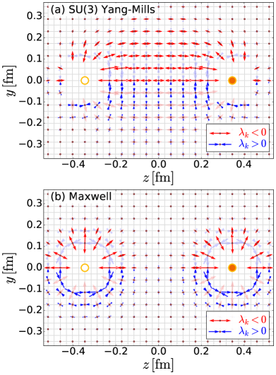
Figure 1: (a) Distribution of the principal axes of ${\cal T}_{ij}$ for a $Q\bar{Q}$ system separated by $R=0.69$ fm in SU(3) Yang-Mills theory. The lattice spacing and the flow time are fixed to be $a=0.029$ fm and $t/a^{2}=2.0$, respectively. (b) Distribution of the principal axes of the ${\cal T}_{ij}$ in classical electrodynamics between opposite charges. In both figures, the red (blue) arrows in the upper (lower) half plane are highlighted.

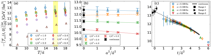
Figure 2: $zz$ component of the stress tensor at $\vec{x}=0$, for various $a$ and $t$ with $R=0.46$ fm. (a) Open symbols with the statistical errors are $\langle{\cal T}_{zz}(t,0)\rangle^{\rm lat}_{Q\bar{Q}}$ as a function of $T/\bar{a}$ with $a=\bar{a}=0.029\ {\rm fm}$. To take the double limit, the data at $T/\bar{a}=16$ indicated by the yellow band is used. (b) Open symbols with errors denote $\langle{\cal T}_{zz}(t,0)\rangle^{\rm lat}_{Q\bar{Q}}$ as a function of $a^{2}/\bar{a}^{2}$. The filled black symbols are the results of the $a\to 0$ limit for each $t$. (c) Open symbols with errors are $\langle{\cal T}_{zz}(t,0)\rangle^{\rm lat}_{Q\bar{Q}}$ as a function of $t/\bar{a}^{2}$ for different $a$. The solid line corresponds to the result of $a\to 0$ limit in the interval $2\leq t/\bar{a}^{2}\leq 5$ with shaded band being statistical error. The filled black symbols are the results of the $t\to 0$ extrapolation from three different ranges of $t$.

We consider three $Q\bar{Q}$ distances ($R=0.46,0.69,0.92$ fm), which are comparable to the typical scale of strong interaction. These values as well as the corresponding dimensionless distances $R/a$ are summarized in Table 1. While the largest $R$ is half the spatial lattice extent $aN_{\rm size}$ for the two finest lattice spacings, effects of the periodic boundary are known to be well suppressed even with this setting [7]. A measure of the ground state saturation in the $Q\bar{Q}$ system reads

$${P}(R,T)={C_{0}(R)e^{-V(R)T}}/{\langle W(R,T)\rangle_{0}}$$ (11)

with the ground-state potential $V(R)$ and the ground-state overlap $C_{0}(R)$ obtained at large $T$  [7]. Using the data at $a=0.038$ fm with $N_{\rm APE}=160$, we found $|1-{P}(R,T)|<{0.5}\%$ as long as $T>0.19$ fm for all $R$ in Table 1. By keeping $T\simeq 0.46$ fm to extract observables as shown in the last column of Table 1, the ground state saturation of the Wilson loop is, therefore, secured in our simulations.

To avoid the artifact due to finite $a$ and the over-smearing of the gradient flow [20, 22], we need to choose an appropriate window of $t$ satisfying the condition ${a}/{2}\lesssim\rho\lesssim L$. Here $\rho\equiv\sqrt{{2t}}$ is the flow radius, and $L\equiv{\rm min}(|\vec{x}-\vec{R}_{+}|,|\vec{x}-\vec{R}_{-}|,T/2)$ is the minimal distance between $x_{\mu}=(\vec{x},0)$ and the Wilson loop.

Before taking the double limit in Eq. (9), we illustrate a qualitative feature of the distribution of ${\cal T}_{ij}$ around $Q\bar{Q}$ in YM theory at fixed $a$ and $t$ by considering the case $a=0.029\ {\rm fm}$ with $R=0.69\ {\rm fm}$, $T=0.46\ {\rm fm}$, and $t/{a}^{2}=2.0$. Shown in Fig. 1 are the two eigenvectors in Eq. (4) along with the principal axes of the local stress. The other eigenvector is perpendicular to the $y$-$z$ plane. The eigenvector with negative (positive) eigenvalue is denoted by the red outward (blue inward) arrow with its length proportional to $\sqrt{|\lambda_{k}|}$:

$${\color[rgb]{1,0,0}\leftarrow}{\tiny{\circ}}{\color[rgb]{1,0,0}\rightarrow}:\lambda_{k}<0,\qquad{\color[rgb]{0,0,1}\rightarrow}{\tiny{\circ}}{\color[rgb]{0,0,1}\leftarrow}:\lambda_{k}>0.$$ (12)

Neighbouring volume elements are pulling (pushing) with each other along the direction of red (blue) arrow according to Eq. (3).

The spatial regions near $Q$ and $\bar{Q}$, which would suffer from over-smearing, are excluded in the figure. Spatial structure of the flux tube is clearly revealed through the stress tensor in Fig. 1 (a) in a gauge invariant way. This is in contrast to the same plot of the principal axes of ${\cal T}_{ij}$ for opposite charges in classical electrodynamics given in Fig. 1 (b).

Let us now turn to the mid-plane between the $Q\bar{Q}$ pair and extract the stress-tensor distribution at $\vec{x}=(x,y,0)$ by taking the double limit Eq. (9). In Fig. 2 (a), we show an example of the $T$ dependence of $\langle{\cal T}_{zz}(t,0)\rangle_{Q\bar{Q}}^{\rm lat}$, which gives the largest eigenvalue on the mid-plane, for several values of $t$ with $a=0.029\ {\rm fm}\ (\equiv\bar{a})$. The figure indicates that significant $T$-dependence arises owing to over-smearing of the gradient flow for $t/\bar{a}^{2}\sim 6$ (i.e., $\rho\sim\sqrt{12}\bar{a}=0.10$ fm) already around $T=16\bar{a}=0.46$ fm. This is so for the same $t/\bar{a}^{2}$ in all other cases in Table 1. On the other hand, under-smearing of the gradient flow on the coarsest lattice becomes significant for $t/\bar{a}^{2}=2$ ($\rho=a=0.058$ fm). Therefore, in the following analysis, we focus on the data in the interval $2\leq t/\bar{a}^{2}\leq 5$ ($2\bar{a}\leq\rho\leq\sqrt{10}\bar{a}$), which satisfies ${a}/{2}\lesssim\rho\lesssim L$ with margin.

In Fig. 2 (b), we show $\langle{\cal T}_{zz}(t,0)\rangle_{Q\bar{Q}}^{\rm lat}$ as a function of the dimensionless ratio $a^{2}/\bar{a}^{2}$ by the open triangles for different values of $t$. The continuum limit ($a\rightarrow 0$) with fixed $t$ is taken by using these data together with the formula Eq. (10). The results are shown by the filled black squares with error bars.

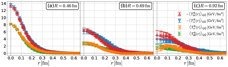
Figure 3: EMT distribution on the mid-plane after the double limit $-\langle{\cal T}^{\rm R}_{cc}(r)\rangle_{Q\bar{Q}}$ and $-\langle{\cal T}^{\rm R}_{44}(r)\rangle_{Q\bar{Q}}$ in the cylindrical coordinate system for three different values of the $Q\bar{Q}$ distance $R$.

In Fig. 2 (c), the open symbols with error bars correspond to the original data for various values of $a$ and $t/\bar{a}^{2}$. The result of the continuum limit in the interval $2\leq t/\bar{a}^{2}\leq 5$ is denoted by the black solid line with the shaded error band. The $t\rightarrow 0$ limit is carried out by using the values in the continuum limit according to Eq. (10) with $a=0$. As a most conservative range for the extrapolation, we take $3\leq t/\bar{a}^{2}\leq 4$ (Range-1). Also, to estimate the systematic errors from the extrapolation, we consider two different ranges by changing the upper and lower limits: $2\leq t/\bar{a}^{2}\leq 4$ (Range-2) and $3\leq t/\bar{a}^{2}\leq 5$ (Range-3). The resulting values of $\langle{\cal T}_{zz}^{\rm R}(0)\rangle_{Q\bar{Q}}$ after the double limit are shown by the filled black symbols at $t=0$. The dashed line corresponds to the extrapolation with Range-1.

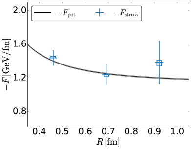
Figure 4: $R$ dependence of the $Q\bar{Q}$ forces, $-F_{\rm stress}$ and $-F_{\rm pot}$, obtained by the Wilson loop and the stress tensor, respectively. Error bars and rectangular boxes for the latter represent the statistical and systematic errors, respectively.

The double limit for general $\vec{x}=(x,y,0)$ on the mid-plane can be carried out essentially through the same procedure with a few extra steps. First of all, the cylindrical coordinate system $c=(r,\theta,z)$ with $r=\sqrt{x^{2}+y^{2}}$ and $0\leq\theta<2\pi$ is useful for the present $Q\bar{Q}$ system. On the mid-plane we have $\langle{\cal T}_{cc^{\prime}}(t,x)\rangle_{Q\bar{Q}}^{\rm lat}={\rm diag}(\langle{\cal T}_{rr}(t,r)\rangle_{Q\bar{Q}}^{\rm lat},\langle{\cal T}_{\theta\theta}(t,r)\rangle_{Q\bar{Q}}^{\rm lat},\langle{\cal T}_{zz}(t,r)\rangle_{Q\bar{Q}}^{\rm lat})$. Next, we need data at the same $r$ for different $a$ to take the continuum limit. We consider the values of $r$ at which the lattice data are available on the finest lattice. To obtain the data at these $r$ on lattices with different $a$, we interpolate the lattice data $\langle{\cal T}_{cc}(t,r)\rangle_{Q\bar{Q}}^{\rm lat}$ and $\langle{\cal T}_{44}(t,r)\rangle_{Q\bar{Q}}^{\rm lat}$ with the commonly used functions to parametrize the transverse profile of the flux tube: $f_{\rm Bessel}(r)=A_{0}K_{0}\big{(}\sqrt{Br^{2}+C}\big{)}$ with the 0th-order modified Bessel function $K_{0}(x)$ [31] and $f_{\rm exp}(r)=(A_{0}+A_{1}r^{2})e^{(-2\sqrt{r^{2}+B^{2}}+2B)/C}$ [13]. Once it is done, the $t\to 0$ limit is taken in the same way as explained above.

In Fig. 3, we show the $r$ dependence of the resulting EMT (the stress tensor $-\langle{\cal T}^{\rm R}_{cc}(r)\rangle_{Q\bar{Q}}$ and the energy density $-\langle{\cal T}^{\rm R}_{44}(r)\rangle_{Q\bar{Q}}$). From the figure, one finds several noticeable features:

• Approximate degeneracy between temporal and longitudinal components is found for a wide range of $r$: $\langle{\cal T}^{\rm R}_{44}(r)\rangle_{Q\bar{Q}}\simeq\langle{\cal T}^{\rm R}_{zz}(r)\rangle_{Q\bar{Q}}<0$. This feature is compatible with the leading-order prediction of the worldsheet theory of QCD string [11]. We also find $\langle{\cal T}^{\rm R}_{rr}(r)\rangle_{Q\bar{Q}}\simeq\langle{\cal T}^{\rm R}_{\theta\theta}(r)\rangle_{Q\bar{Q}}>0$, which does not have simple interpretation except at $r=0$.

• The scale symmetry broken in the YM vacuum (the trace anomaly) is partially restored inside the flux tube, which arises in the numerical results, $\langle{\cal T}^{\rm R}_{\mu\mu}(r)\rangle_{Q\bar{Q}}=\langle{\cal T}^{\rm R}_{44}(r)+{\cal T}^{\rm R}_{zz}(r)+{\cal T}^{\rm R}_{rr}(r)+{\cal T}^{\rm R}_{\theta\theta}(r)\rangle_{Q\bar{Q}}<0$. This is in sharp contrast to the case of classical electrodynamics; ${\cal T}_{44}(r)={\cal T}_{zz}(r)=-{\cal T}_{rr}(r)=-{\cal T}_{\theta\theta}(r)$ and ${\cal T}_{\mu\mu}(r)=0$ for all $r$.

• Each component of EMT at $r=0$ decreases as $R$ becomes larger, while the transverse radius of the flux tube, typically about $0.2$ fm, seems to increase for large $R$ [13, 23, 10], although the statistics is not enough to discuss the radius quantitatively.

Finally, we consider a non-trivial relation between the force acting on the charge located at $z>0$ evaluated by the $Q\bar{Q}$ potential through

$$F_{\rm pot}=-dV(R)/dR$$ (13)

and the force evaluated by the surface integral of the stress-tensor surrounding the charge,

$$F_{\rm stress}=-\int\langle{\cal T}_{zj}(x)\rangle_{Q\bar{Q}}\ dS_{j}.$$ (14)

For $F_{\rm pot}$, we fit the numerical data of $V(R)$ obtained from the Wilson loop at $a=0.038$ fm by the Cornell parametrization, $V_{\rm Cornell}(R)=-{\cal A}/R+\sigma R+{\cal B}$. Note that $V(R)$ at this lattice spacing is shown to be already close to the continuum limit [3]. For $F_{\rm stress}$, we take the mid-plane for the surface integral: $F_{\rm stress}=2\pi\int_{0}^{\infty}\langle{\cal T}_{zz}(r)\rangle_{Q\bar{Q}}\ rdr$. Here $\langle{\cal T}_{zz}(r)\rangle_{Q\bar{Q}}$ is obtained by fitting Fig. 3 with either $f_{\rm Bessel}(r)$ or $f_{\rm exp}(r)$. In Fig. 4, $-F_{\rm pot}$ and $-F_{\rm stress}$ thus obtained are shown by the solid line and the horizontal bars, respectively. $-F_{\rm pot}$ increases as ${\cal A}/R^{2}$ at short distance and approaches the string tension $\sigma$ at large distance. For $-F_{\rm stress}$, we take into account not only the statistical error but also the systematic errors from the double limit and the fitting in terms of $f_{\rm Bessel,exp}(r)$. The agreement between the two quantities within the errors is a first numerical evidence that the “action-at-a-distance” $Q\bar{Q}$ force can be described by the local properties of the stress tensor in YM theory.

In this Letter, we have performed a first study on the spatial distribution of EMT around the $Q\bar{Q}$ system in SU(3) lattice gauge theory. The EMT operator defined through the YM gradient flow plays a crucial role here. The transverse structure of the stress-tensor distribution in the mid-plane is analyzed in detail by taking the continuum limit and the zero flow-time limit successively. The linear confining behavior of the $Q\bar{Q}$ potential at long distances can be shown to be reproduced by the surface integral of the stress tensor. Further details of the stress-tensor distribution, not only in the transverse direction but also in the longitudinal direction, and $R$ dependence of the transverse radius [13, 23, 10], will be reported in a forthcoming publication [32]. There are also interesting future problems to be studied on the basis of the formalism presented in this Letter: Those include the applications to the $QQQ$ system [27] and to the $Q\bar{Q}$ system at finite temperature [33] as well as the generalization to full QCD [34] with the QCD flow equation [35, 36].

The authors thank K. Kondo, F. Negro, A. Shibata, and H. Suzuki for discussions. Numerical simulation was carried out on IBM System Blue Gene Solution at KEK under its Large-Scale Simulation Program (No. 16/17-07). This work was supported by JSPS Grant-in-Aid for Scientific Researches, 17K05442, 25287066 and 18H05236. T.H. is grateful to the Aspen Center for Physics, supported in part by NSF Grants PHY1607611.

References

- [1] L. D. Landau and E. M. Lifshitz, “The Classical Theory of Fields” (fourth Edition) §32, §33, §35 (Butterworth-Heinemann, 1980).
- [2] Y. Nambu, Phys. Rev. D10, 4262 (1974); Phys. Lett. B80, 372 (1979). S. Mandelstam, Phys. Rep. 23C, 245 (1976). G. ’t Hooft, in High Energy Physics, Proceedings of the European Physical Society Conference, Palermo, 1975, ed. A. Zichichi (Editrice Compositori, Bologna, 1976).
- [3] G. S. Bali, Phys. Rept. 343, 1 (2001).
- [4] J. Greensite, Lect. Notes. Phys. 821, 1 (2011).
- [5] K. I. Kondo, S. Kato, A. Shibata, and T. Shinohara, Phys. Rept. 579, 1 (2015) [arXiv:1409.1599 [hep-th]].
- [6] A. Di Giacomo, M. Maggiore, and S. Olejnik, Nucl. Phys. B 347, 441 (1990).
- [7] G. S. Bali, K. Schilling, and C. Schlichter, Phys. Rev. D 51, 5165 (1995) [hep-lat/9409005].
- [8] C. Michael, Phys. Rev. D 53, 4102 (1996) [hep-lat/9504016].
- [9] A. M. Green, C. Michael and P. S. Spencer, Phys. Rev. D 55, 1216 (1997) [hep-lat/9610011].
- [10] F. Gliozzi, M. Pepe and U.-J. Wiese, Phys. Rev. Lett. 104, 232001 (2010) [arXiv:1002.4888 [hep-lat]].
- [11] H. B. Meyer, Phys. Rev. D 82, 106001 (2010) [arXiv:1008.1178 [hep-lat]].
- [12] P. Cea, L. Cosmai, and A. Papa, Phys. Rev. D 86, 054501 (2012) [arXiv:1208.1362 [hep-lat]].
- [13] N. Cardoso, M. Cardoso, and P. Bicudo, Phys. Rev. D 88, 054504 (2013) [arXiv:1302.3633 [hep-lat]].
- [14] R. Narayanan and H. Neuberger, JHEP 0603, 064 (2006) [hep-th/0601210].
- [15] M. Lüscher, JHEP 1008, 071 (2010) [arXiv:1006.4518 [hep-lat]].
- [16] M. Lüscher and P. Weisz, JHEP 1102, 051 (2011) [arXiv:1101.0963 [hep-th]].
- [17] H. Suzuki, PTEP 2013, no. 8, 083B03 (2013) [Erratum: PTEP 2015, no. 7, 079201 (2015)] [arXiv:1304.0533 [hep-lat]].
- [18] H. Suzuki, PoS LATTICE 2016, 002 (2017) [arXiv:1612.00210 [hep-lat]], and references therein.
- [19] M. Asakawa et al. [FlowQCD Collaboration], Phys. Rev. D 90, 011501 (2014) [Erratum: Phys. Rev. D 92, no. 5, 059902 (2015)] [arXiv:1312.7492 [hep-lat]].
- [20] M. Kitazawa, T. Iritani, M. Asakawa, T. Hatsuda, and H. Suzuki, Phys. Rev. D 94, 114512 (2016) [arXiv:1610.07810 [hep-lat]].
- [21] N. Kamata and S. Sasaki, Phys. Rev. D 95, no. 5, 054501 (2017) [arXiv:1609.07115 [hep-lat]].
- [22] M. Kitazawa, T. Iritani, M. Asakawa, and T. Hatsuda, Phys. Rev. D 96, 111502 (2017) [arXiv:1708.01415 [hep-lat]].
- [23] M. Lüscher, G. Münster, P. Weisz, Nucl. Phys. B180, 1 (1981).
- [24] M. G. Endres, PoS LATTICE 2016, 014 (2016) [arXiv:1612.01609 [hep-lat]].
- [25] S. Borsanyi, S. Dürr, Z. Fodor et al., JHEP 1209, 010 (2012) [arXiv:1203.4469 [hep-lat]].
- [26] M. Albanese et al. [APE Collaboration], Phys. Lett. B 192, 163 (1987).
- [27] T. T. Takahashi, H. Suganuma, Y. Nemoto, and H. Matsufuru, Phys. Rev. D 65, 114509 (2002) [hep-lat/0204011].
- [28] G. Parisi, R. Petronzio, and F. Rapuano, Phys. Lett. 128B, 418 (1983).
- [29] M. Lüscher and P. Weisz, JHEP 0207, 049 (2002). [hep-lat/0207003].
- [30] K. J. Juge, J. Kuti and C. Morningstar, Phys. Rev. Lett. 90, 161601 (2003). [hep-lat/0207004].
- [31] J.R. Clem, J. Low Temp. Phys. 18, 427 (1975).
- [32] R. Yanagihara, et al., in preparation.
- [33] P. Cea, L. Cosmai, F. Cuteri, and A. Papa, JHEP 1606, 033 (2016) [arXiv:1511.01783 [hep-lat]].
- [34] P. Cea, L. Cosmai, F. Cuteri, and A. Papa, Phys. Rev. D 95, 114511 (2017) [arXiv:1702.06437 [hep-lat]].
- [35] H. Makino and H. Suzuki, PTEP 2014, no. 6, 063B02 (2014) [Erratum: PTEP 2015, no. 7, 079202 (2015)] [arXiv:1403.4772 [hep-lat]].
- [36] Y. Taniguchi, S. Ejiri, R. Iwami, K. Kanaya, M. Kitazawa, H. Suzuki, T. Umeda, and N. Wakabayashi, Phys. Rev. D 96, 014509 (2017) [arXiv:1609.01417 [hep-lat]].