TTP99–22
hep-ph/9905298
May 1999

Automatic application of successive asymptotic expansions of Feynman diagrams

Abstract

We discuss the program EXP used to automate the successive application of asymptotic expansions to Feynman diagrams. We focus on the generation of the relevant subgraphs and the determination of the topologies for the remaining integrals. Both tasks can be solved by using backtracking-type recursive algorithms. In addition, an application of EXP is presented, where the integrals were calculated using the FORM packages MINCER and MATAD.

1 Introduction

The necessity of calculating higher order corrections to physical processes is based on the increasing precision of experimental data. Unfortunately, analytic expressions for higher order corrections are in most cases out of reach. This is mainly due to the fact that the integrals contain several different mass scales.

One possible approach to tackle the problem is based on the procedures of asymptotic expansions (see, e.g. [1] and references therein) which provide rules for consistent expansions of Feynman diagrams in large scales. If a certain hierarchy between the different mass scales can be found for a given diagram one expands with respect to a small quantity. Although the complexitity of the remaining integrals is reduced by the asymptotic expansion sometimes those integrals cannot be solved analytically either. To further proceed in these cases we repeat the application of an expansion procedure using another large scale. Consequently the final result is expressed in terms of nested series in small quantities.

In this paper we discuss algorithms we used to automate the successive application of asymptotic expansions. The algorithms were implemented in the C++ program EXP. The output files of EXP can be directly used by a skeleton FORM [2] mainfile. The mainfile is based on the integration packages MINCER [3] and MATAD [4] which perform the actual integrations for single scale integrals up to three loops. Also some administrative files like make-files are written by EXP.

2 Asymptotic expansions

Let us begin by listing the rules of the asymptotic expansions which are expressed in a purely diagrammatic manner. They can be divided into two parts: First, the rules for the selection of all relevant so-called hard subgraphs and second, how to expand the propagators of the hard subgraphs.

In case of expansions with respect to a large mass (the so-called hard mass procedure) one has to find all hard subgraphs which contain all lines carrying the large mass and are one-particle-irreducible with respect to light lines in their connected parts. The propagators appearing in the hard subgraph have to be expanded with respect to small masses and external momenta.

Expansions with respect to a large momentum (large momentum procedure) can be obtained in a similar way. The hard subgraphs must contain the vertices with the large external momentum and become one-particle-irreducible if those vertices are identified. The propagators have to be expanded with respect to masses and external momenta generated by removing lines from the initial diagram.

The final result for a given diagram is obtained in four steps:

(1) Shrink the lines of the hard subgraph to a point. The remaining diagram is called co-subgraph.

(2) Expand the propagators and (if necessary) do the integrals in the hard subgraph. Insert the result into the co-subgraph.

(3) Calculate the remaining integrals in the co-subgraph.

(4) Sum over all terms.

The number of relevant subdiagrams increases rapidly with the number of loops of the initial diagram especially when we deal with successive asymptotic expansions. Providing all necessary information by hand is nearly impossible and automation is an obvious task.

Figure 1: Double triangle graphs contributing to $\Gamma(H\rightarrow b\bar{b})$.

3 Example

To illustrate the successive application of asymptotic expansions we consider the singlet contributions of ${\cal O}(\alpha_{s}^{2})$ to the decay of a scalar Higgs boson into bottom quarks. Instead of calculating the vertex diagrams, we use the optical theorem and compute the imaginary part of the Higgs boson propagator to three loops. There are four diagrams relevant for this problem, two are shown in figure 1. The dashed lines denote the Higgs boson of mass $M_{H}$, the thick lines represent top quarks ($M_{t}$), the thin lines bottom quarks ($M_{b}$) and the curly lines are gluons. The remaining two diagrams have crossed gluon lines and their contribution can be included by an additional factor of 2 in the result. This problem has been analyzed in [5, 6]. We used the results given in [5] as a check for the program EXP.

Suppose we want to compute the singlet contribution for a Higgs boson mass smaller than the mass of the top quark. Then we have to choose the hierarchy

$$M_{t}^{2}\gg q^{2}=M_{H}^{2}\gg M_{b}^{2},$$

where $q$ denotes the external momentum. Therefore we have to compute an expansion with respect to a large mass ($M_{t}^{2}$) followed by an expansion with respect to a large momentum ($q^{2}=M_{H}^{2}$).

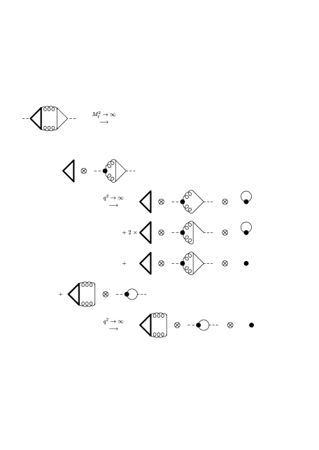
If we restrict ourselves to the imaginary part of the Higgs boson propagator, the hard subgraphs for diagram 1(a) are shown in figure 2. The application of the hard mass procedure with respect to $M_{t}$ results in two hard subgraphs shown on the left hand side of figure 2.

In the upper case, the original integral factorizes into a 1-loop tadpole (hard subgraph) and a 2-scale 2-loop integral (co-subgraph) which has to be expanded in the next step with respect to the large momentum $q^{2}$. Note that there is a contribution from the naive Taylor expansion with respect to the bottom quark mass $M_{b}$ (last line of upper case). In the lower case, the result is a product of a 2-loop tadpole and a 2-scale 1-loop integral. The 2-scale integral can be solved analytically. Since we use the packages MINCER and MATAD – dealing with single scale integrals – the co-subgraph has to be expanded as well.

Figure 2: Successive asymptotic expansion of diagram 1(a).

4 Generation of subgraphs

In this section we will shortly discuss the algorithms used for the generation of the relevant subgraphs. The main data structure used in the implementation of EXP is a graph represented by a set of lines which are in turn represented as connections of vertices.

We use a prototype backtracking algorithm to generate all possible subsets of lines. For each subset the conditions for hard subgraphs given by the current procedure are tested. Since these rules are mainly based on the property “one-particle-irreducible” we must develop a general prescription for this to construct an algorithm.

A graph is one-particle-irreducible if cutting an arbitrary line does not split the graph into two distinct parts. Therefore every vertex should still be connected to all the other vertices after removing one line. That means that one can find a route through the graph given by a sequence of lines to get from one vertex to the other. The procedure of finding such a route between two vertices can be realised quite elegantly using a recursive algorithm: One starts at a given vertex and determines all vertices directly (by one line) connected to it. Then one recursively tries to find a connection between the directly connected vertices and the target vertex. Thus all possible routes through the graph are taken into account.

Further limitations implied by the rules of asymptotic expansion can be easily implemented since they restrict only the type of lines to be cut or the subset of vertices to be connected after cutting a line.

5 Determination of topologies

Our approach for the determination of the topologies is based on the observation that the combinations of external and loop momenta in the lines of the graph can be used to identify the topology. The idea is to compare a given distribution of momenta to all possible ones for a certain number of standard topologies which can (or must) be defined by the user.

The determination of a topology can be divided into four parts:

(1) A momentum distribution is computed for each individual subgraph. Note that not all possible choices are suitable for our problem since the propagators must be expanded in taylor series.

(2) The rules for the expansion of the propagators are applied. This is done by setting marks on momenta and masses which have to be expanded. Marked quantities will be ignored during the next steps, because they are obviously irrelevant for the determination of topologies. The real expansion is, of course, done later using FORM. Lines sharing the same loop momenta are sorted into groups which correspond to different types of integrals.

(3) All possible distributions of momenta for the standard topologies are computed and the coefficients of the external and loop momenta are compared to those calculated for the lines in the current subset. This comparison of the external and loop momenta fixes the topologies with respect to the number of loops and external momenta.

(4) As the last step, the masses of the propagators will be compared to those defined in the standard topology.

The computation of all possible distributions of momenta which is the crucial part of the algorithm described above is done by recursively assigning loop momenta to certain lines, i.e. by defining that certain lines should carry the loop momenta and solving the linear set of equations given by the conservation of momentum at each vertex. Therefore we restrict ourselves to distributions of momenta with integer coefficients for external and loop momenta which is sufficient for our problem.

There will be cases where the algorithm fails to find a topology for a group of lines. These lines will be separated from the full graph and an asymptotic expansion is applied again, until all integrals can be expressed in terms of standard topologies.

The hierarchy of mass scales for all expansions must be defined by the user.

In principle, this algorithm is not limited with respect to the number of loops or external momenta as long as the user supplies a sufficient amount of standard topologies.

6 Example: result

In this section we list the result for the imaginary part of the diagrams considered in section 3 expressed in terms of a nested series in the the variables $M_{H}^{2}/M_{t}^{2}$ and $M_{b}^{2}/M_{H}^{2}$. It reads:

$$\Gamma^{sing}(H\rightarrow b\bar{b},gluons)={{N_{C}\,M_{H}\,\alpha}\over s_{W}^{2}}\,{M_{b}^{2}\over M_{W}^{2}}\,\bigg{(}{\alpha_{s}\over\pi}\bigg{)}^{2}\,C_{F}T\times$$ (1)

$$\mbox{}\bigg{\{}{7\over 12}+{1\over 8}\,L_{tH}+{M_{b}^{2}\over M_{H}^{2}}\,\bigg{(}-{3\over 8}-{3\over 4}\,L_{tH}-{1\over 4}\,L_{Hb}\bigg{)}+{M_{H}^{2}\over M_{t}^{2}}\,\bigg{(}{2011\over 129600}+{41\over 8640}\,L_{tH}\bigg{)}$$

$$\mbox{}+{M_{b}^{2}\over M_{t}^{2}}\bigg{(}{713\over 14400}+{7\over 1440}\,L_{tH}+{1\over 288}\,L_{Hb}\bigg{)}+\bigg{(}{M_{H}^{2}\over M_{t}^{2}}\bigg{)}^{2}\,\bigg{(}{28307\over 25401600}+{47\over 120960}\,L_{tH}\bigg{)}$$

$$\mbox{}+{{M_{b}^{2}\,M_{H}^{2}}\over M_{t}^{4}}\bigg{(}{10901\over 25401600}+{1\over 1080}\,L_{tH}\bigg{)}+{\cal O}(M_{b}^{4})+{\cal O}(M_{t}^{-6})\bigg{\}},$$

with $L_{tH}=\ln(M_{t}^{2}/M_{H}^{2})$ and $L_{Hb}=\ln(M_{H}^{2}/M_{b}^{2})$. $N_{C}$ denotes the number of colours and $s_{W}$ is the sine of the weak mixing angle; $T=1/2$ and $C_{F}=(N_{C}^{2}-1)/(2N_{C})$. Using EXP we were able to add the terms proportional to $M_{t}^{-4}$ to the result given in [5]. Numerically they are small compared to the leading terms.

The notation $\Gamma^{sing}(H\rightarrow b\bar{b},gluons)$ has been chosen, because the diagrams shown in figure 1 contain contributions from cuts through the two gluon lines. These have to be subtracted if one is not interested in the total decay rate and are known analytically to this order [7].

There are two important checks for the result: First, it must be independent of the choice of the QCD gauge parameter. Second, since the diagrams shown in figure 1 contain no divergent subgraphs their imaginary part must be finite without further renormalization.

Acknowlegements

We would like to thank K.G. Chetyrkin, R. Harlander, J.H. Kühn and M. Steinhauser for fruitful discussions and advice, and D. Fliegner for carefully reading the manuscript. This work was supported by the DFG-Forschergruppe ”Quantenfeldtheorie, Computeralgebra und Monte-Carlo-Simulationen”, the Landesgraduiertenförderung and the Graduiertenkolleg ”Elementarteilchenphysik” at the University of Karlsruhe.

References

- [1] V.A. Smirnov, Commun. Math. Phys. 139 (1990) 109;
- [2] J.A.M. Vermaseren, Symbolic Manipulation with FORM, CAN (1991).
- [3] S.A. Larin, F.V. Tkachov and J.A.M. Vermaseren, Preprint NIKHEF-H/91-18 (1991).
- [4] M. Steinhauser, PhD thesis, University of Karlsruhe, Shaker Verlag, Aachen, 1996.
- [5] K.G Chetyrkin und A. Kwiatkowski, Nucl. Phys. B 461 (1996) 3.
- [6] S.A. Larin, T. van Ritbergen, J.A.M. Vermaseren, Phys. Lett. B 362 (1995) 134.
- [7] J. Ellis, M. Gaillard und D.V. Nanopoulos, Nucl. Phys. B 106 (1976) 292.