Magnetohydrodynamic Fast Sausage Waves in the Solar Corona

Abstract

Characterized by cyclic axisymmetric perturbations to both the magnetic and fluid parameters, magnetohydrodynamic fast sausage modes (FSMs) have proven useful for solar coronal seismology given their strong dispersion. This review starts by summarizing the dispersive properties of the FSMs in the canonical configuration where the equilibrium quantities are transversely structured in a step fashion. With this preparation we then review the recent theoretical studies on coronal FSMs, showing that the canonical dispersion features have been better understood physically, and further exploited seismologically. In addition, we show that departures from the canonical equilibrium configuration have led to qualitatively different dispersion features, thereby substantially broadening the range of observations that FSMs can be invoked to account for. We also summarize the advances in forward modeling studies, emphasizing the intricacies in interpreting observed oscillatory signals in terms of FSMs. All these advances notwithstanding, we offer a list of aspects that remain to be better addressed, with the physical connection of coronal FSMs to the quasi-periodic pulsations in solar flares particularly noteworthy.

1 Introduction

Despite the considerable advances in modern instrumentation, it remains challenging to directly measure some key parameters of the highly structured solar corona, the magnetic field being particularly noteworthy (e.g., Cargill 2009). Coronal seismology has proven valuable for indirectly probing coronal structures by combining the measurements of the hosted low-frequency waves with continuously refined theories of magnetohydrodynamic (MHD) waves in an inhomogeneous medium (Roberts et al. 1984, see also the reviews by e.g., Roberts 2000, Nakariakov and Verwichte 2005, Nakariakov and Kolotkov 2020). The terminology in modern coronal seismology comes primarily from the theoretical work by Edwin and Roberts (1983, hereafter ER83). Among the many “collective waves” (“modes” hereafter), sausage modes are the simplest in that the associated perturbations are axisymmetric, but prove theoretically intriguing and seismologically important given their dispersion. Take fast sausage modes (FSMs) for instance, which will be the focus of this review. Theoretically, two intriguing features arise, one being that FSMs can be trapped only when their axial wavenumbers exceed some cutoff (Roberts et al. 1984), the other being that their axial group speed possesses a nonmonotonic frequency dependence (Roberts et al. 1983). The former feature leads to the periods of standing FSMs being comparable to the transverse Alfv$\acute{\rm e}$n time. For impulsively excited sausage wavetrains, the two features lead to a distinctive temporal profile comprising a periodic phase, a quasi-periodic phase, and an Airy (decay) phase when the profile is sampled sufficiently far from the exciter. Regardless, the characteristic periodicity remains similar to the transverse Alfv$\acute{\rm e}$n time, which evaluates to seconds to tens of seconds for typical coronal structures. Consequently, FSMs in flare-associated structures were proposed to interpret second-scale oscillations often seen in type IV radio bursts (Roberts et al. 1983, see also Rosenberg 1970, Zajtsev and Stepanov 1975, Meerson et al. 1978 ). This interpretation remains popular today (e.g., Karlický et al. 2013; Kaneda et al. 2018), and has been generalized to be a strong candidate mechanism for interpreting and seismologically exploiting short-period Quasi-Periodic Pulsations (QPPs) in flare lightcurves (see e.g., the reviews by Nakariakov and Melnikov 2009, Van Doorsselaere et al. 2016, McLaughlin et al. 2018, Kupriyanova et al. 2020; also the review by Zimovets et al. in this issue). Likewise, impulsively generated wavetrains have been generalized to account for short-period oscillatory signals associated with active region (AR) loops observed in white light and various coronal forbidden lines at total eclipses (e.g. Pasachoff and Landman 1984; Pasachoff and Ladd 1987; Williams et al. 2001, 2002; Katsiyannis et al. 2003; Samanta et al. 2016).

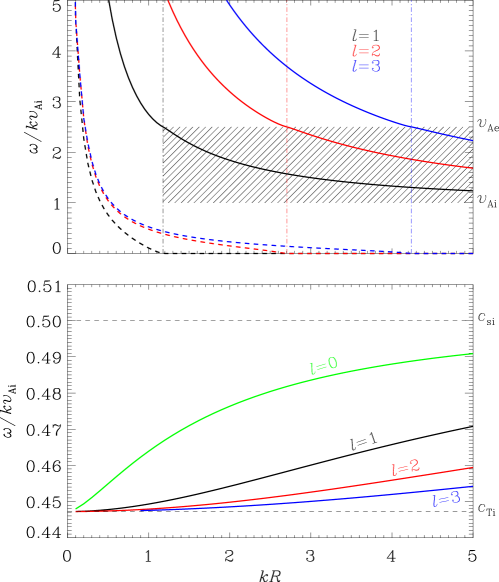
Figure 1: Dependence on the axial wavenumber $k$ of the axial phase speed ($\omega/k$) for (a) fast and (b) slow sausage modes in the cylindrical equilibrium considered by Edwin and Roberts (1983, ER83). Here $[c_{\rm si},c_{\rm se},v_{\rm Ae}]=[0.5,0.25,2.5]~{}v_{\rm Ai}$, where $c_{\rm s}$ ($v_{\rm A}$) is the adiabatic sound (Alfv$\acute{\rm e}$n) speed, and the subscript i (e) denotes the values at the loop axis (far from the loop). This ordering of the characteristic speeds is typical of coronal conditions. The solid and dashed curves derive from the real ($\omega_{\rm R}$) and imaginary ($\omega_{\rm I}$) parts of the angular frequency. Note that $\omega_{\rm I}$ is identically zero for trapped modes, and $-\omega_{\rm I}$ is employed to produce the dashed curves in Figure 1a. Slow modes are trapped regardless of $k$, whereas fast modes are trapped only when $k$ exceeds some cutoff as seen in the hatched area. This figure is essentially a combination of Figure 4 in ER83, Figure 1 in Kopylova et al. (2007), and Figure 6 in Van Doorsselaere et al. (2016).

This review is intended to summarize recent advances in the theoretical understanding and consequently seismological applications of coronal FSMs. Before proceeding, however, with AR loops and flare loops in mind, let us list some typical ranges of the values for the length-to-radius ratio ($L/R$), plasma $\beta$, and the density contrast between the loop fluid and its surroundings. For AR loops imaged in EUV and soft X-ray, the loop length ($L$) typically lies in the range of $[20,1000]~{}{\rm Mm}$, while the half-width ($R$) is $\lesssim 5~{}{\rm Mm}$ (Schrijver 2007, Figure 1) and may reach down to $\lesssim 300$ km (Aschwanden and Peter 2017). Therefore one typically quotes $L/R\gtrsim 10-20$ for AR loops, whereas $L/R$ was suggested to be smaller for flare loops (Aschwanden et al. 2004). The value of $L/R$ for flare loops is actually passband-dependent, with values as small as $\lesssim 5$ reported in radio measurements with NoRH (e.g., Kupriyanova et al. 2013). As for the density contrast, values of $2-10$ are usually quoted for AR loops, while a value up to $100-1000$ is possible for flare loops (Aschwanden et al. 2004). Furthermore, a value of $\beta\lesssim 1$ or even $\beta\ll 1$ is accepted for coronal gases across ARs at heights $\lesssim 0.2~{}R_{\odot}$ (Gary 2001), and is usually quoted for AR loops as well. Flare loops are somehow different from this overall picture of a magnetically dominated corona. In the aftermath of the impulsive energy release, the enhanced thermal pressure in some loop segment may be sufficiently dynamically important to expand the segment, leading to a plasma $\beta$ of order unity therein. This thermal pressure enhancement may result directly from the energy release (Zaitsev and Stepanov 1982) or indirectly from the collisions between counter-flowing plasmas that in turn derive from chromospheric evaporation (e.g., Fang et al. 2016; Ruan et al. 2019).

Organizing the recent literature on a subject as specific as coronal FSMs is not easy. We choose to start with an in-depth review of the sausage modes in the ER83 equilibrium (Sect. 2.1), then come up with a list of primary dispersion features and ask what simplifications or complications to the ER83 equilibrium are unlikely to qualitatively modify these features (Sect. 2.2). We will also overview a number of important issues that remain largely unanswered, the excitation of FSMs as an example (Sect. 2.3). Section 3 summarizes the advances in forward modeling coronal FSMs, emphasizing its role for properly interpreting observations (Sect. 3). We will then organize the recent theoretical progress by addressing those modifications to the ER83 equilibrium that result in qualitative modifications to the dispersion features (Sect. 4). Some illustrative seismological applications enabled by these modifications are offered in Section 5. This review is summarized in Section 6, where some possible ways forward are also discussed.

2 Sausage Modes in the ER83 and ER83-like Equilibria

Unless otherwise specified, this review adopts ideal MHD as the theoretical framework, for which the primary dependents are the mass density $\rho$, velocity $\bm{v}$, magnetic field $\bm{B}$, and thermal pressure $p$. Let subscript $0$ denote the equilibrium parameters, from which the plasma $\beta$ is defined by $2\mu_{0}p_{0}/B_{0}^{2}$ with $\mu_{0}$ being the magnetic permeability in free space. The Alfv$\acute{\rm e}$n and adiabatic sound speeds are defined as $v_{\rm A}=B_{0}/\sqrt{\mu_{0}\rho_{0}}$ and $c_{\rm s}=\sqrt{\gamma p_{0}/\rho_{0}}$, respectively. Here $\gamma=5/3$ is the adiabatic index. The tube speed and transverse fast speed are further defined by $c_{\rm T}^{2}=c_{\rm s}^{2}v_{\rm A}^{2}/(c_{\rm s}^{2}+v_{\rm A}^{2})$ and $v_{\rm f}^{2}=c_{\rm s}^{2}+v_{\rm A}^{2}$, respectively.

2.1 Theoretical Basics and Seismological Applications of Sausage Modes in the ER83 Equilibrium

ER83 modeled a coronal loop as a straight, static , density-enhanced, field-aligned tube with circular cross-section, enabling the natural choice of a cylindrical coordinate system $(r,\theta,z)$. All equilibrium parameters depend on $r$ in a step (piece-wise constant) fashion. Standard eigen-mode analysis starts by Fourier-decomposing any perturbation as

$$\delta f(r,\theta,z;t)={\rm Re}\left\{\tilde{f}(r)\exp\left[-i\left(\omega t-kz-m\theta\right)\right]\right\}~{},$$ (1)

where $\omega$, $k$, and $m$ represent the angular frequency, axial wavenumber, and azimuthal wavenumber, respectively. With tilde we denote the Fourier amplitude. This equilibrium allows both incompressible (Alfv$\acute{\rm e}$n) and compressible waves. Among the Alfv$\acute{\rm e}$n waves, the $m=0$ (torsional) and $m=1$ ones are relevant. Among the compressible waves, relevant are the kink ($m=1$) and sausage modes ($m=0$) . We take $k$ as real-valued, but allow $\omega$ to be complex-valued. If some quantity is complex, we denote its real (imaginary) part with subscript R (I). The period $P$ (damping time $\tau$) follows from $P=2\pi/\omega_{\rm R}$ ($\tau=1/|\omega_{\rm I}|$). Instabilities are not of interest, hence $\omega_{\rm I}\leq 0$. The axial phase and group speeds are defined by $v_{\rm ph}=\omega/k$ and $v_{\rm gr}={\rm d}\omega/{\rm d}k$, respectively. For standing modes in a loop with length $L$, the axial wavenumber $k$ is quantized ($k=n\pi/L,n=1,2,\cdots$). We follow the convention that $n=1$ represents the axial fundamental, with $n\geq 2$ representing its $(n-1)$-th harmonic.

Let the subscripts ${\rm i}$ and ${\rm e}$ denote the equilibrium values at the loop axis and far from the loop, respectively . As in ER83, by “coronal conditions” we refer to the ordering $c_{\rm se}<c_{\rm si}<v_{\rm Ai}<v_{\rm Ae}$. The dispersion relation (DR) for sausage modes reads

$$\frac{\rho_{\rm i}J_{0}(\mu_{\rm i}R)(\omega^{2}-k^{2}v_{\rm Ai}^{2})}{\mu_{\rm i}J_{1}(\mu_{\rm i}R)}=\frac{\rho_{\rm e}H^{(1)}_{0}(\mu_{\rm e}R)(\omega^{2}-k^{2}v_{\rm Ae}^{2})}{\mu_{\rm e}H^{(1)}_{1}(\mu_{\rm e}R)}~{},$$ (2)

where

$$\mu_{\rm i,e}^{2}=\frac{(\omega^{2}-k^{2}v_{\rm Ai,e}^{2})(\omega^{2}-k^{2}c_{\rm si,e}^{2})}{(c_{\rm si,e}^{2}+v_{\rm Ai,e}^{2})(\omega^{2}-k^{2}c_{\rm Ti,e}^{2})}~{},$$ (3)

and $J_{n}$ and $H_{n}^{(1)}$ are the $n$-th-order Bessel and Hankel functions of the first kind, respectively (here $n=0,1$). This DR was independently derived by Zajtsev and Stepanov (1975), Spruit (1982), and Cally (1986). It differs in form from the independent ER83 result in that, while ER83 required the perturbations be evanescent in the ambient, Equation (2) allows the perturbations to propagate outward. Trapped modes arise in the former case, where $\mu_{\rm e}^{2}<0$ and $\omega$ is real. Leaky modes arise in the latter case, where $\omega_{\rm I}$ does not vanish.

Figure 1 presents the dependence of the axial phase speed $\omega/k$ on the axial wavenumber $k$ as found by solving the DR (Equation 2). For illustration purposes, here the characteristic speeds are specified as $[c_{\rm si},c_{\rm se},v_{\rm Ae}]=[0.5,0.25,2.5]~{}v_{\rm Ai}$. The real and imaginary parts are plotted by the solid and dashed curves, respectively. For completeness, slow sausage modes (SSMs) are shown (Figure 1b) in addition to FSMs (Figure 1a), the purpose being to show that there are an infinite number of branches, labeled by the transverse order $l$ and plotted by the different colors for both families. The smaller an $l$ is, the simpler the spatial distribution of the eigen-functions. SSMs are trapped regardless of $k$ or $l$, whereas FSMs are trapped only when $k$ exceeds some $l$-dependent cutoff, pertaining to the shaded area in Figure 1a. In addition, $\mu_{\rm i}^{2}>0$ for SSMs and trapped FSMs alike, enabling ER83 to classify them as “body modes”. The peculiar label $l=0$ for SSMs, not present for FSMs, is for mathematical reasons. When $l\geq 1$, for the $l$-th FSM, $\mu_{\rm i}R$ increases monotonically from $j_{0,l}$ at the cutoff to $j_{1,l}$ for $kR\gg 1$, with $j_{n,l}$ representing the $l$-th zero of the Bessel function $J_{n}$ . For the $l$-th SSM, on the other hand, $\mu_{\rm i}R\approx j_{1,l}$ in the thin-tube limit ($kR\ll 1$). For the peculiar $l=0$ branch of SSMs, $\mu_{\rm i}$ for $kR\ll 1$ weakly depends on $kR$ through the appearance of $\ln(kR)$, making its $k$-dependence of $\omega/k$ different from the rest.

The reason for us to make a digression to coronal SSMs, the only digression in this review, is to make a better connection to the companion reviews on slow waves (Banerjee et al. and Wang et al.) in this topical issue. Let $\Delta\rho$ denote the magnitude of the internal density perturbation in units of the internal density $\rho_{\rm i}$. Furthermore, let $\Delta R$ denote the magnitude of the Lagrangian displacement at the loop boundary in units of the loop radius $R$. Likewise, let $\Delta v_{z}$ and $\Delta v_{r}$ denote the magnitudes of the axial and radial speeds, respectively. Extending the analysis in Yu et al. (2016a), it can be shown that $\Delta\rho/\Delta R>4/(\gamma\beta_{\rm i})=2.4/\beta_{\rm i}$ for the branch labeled $l=0$, while taking extremely large values for $l\geq 1$. In addition, $\Delta v_{z}/\Delta v_{r}$ exceeds $2[1+2/(\gamma\beta_{\rm i})]/(kR)$ for $l=0$, and is even larger for $l\geq 1$. Given that $kR\ll 1$ holds in typical observations of coronal SSMs, this means that it is extremely difficult to discern the associated expansion or contraction of the loop in imaging observations. Likewise, in spectroscopic measurements, the oscillatory behavior in Doppler shift in general derives from the periodic variations in the axial flow. Physically, it is in general justified to see slow sausage modes as field-guided sound waves. This substantially simplifies the relevant efforts for modeling both the slow waves themselves (e.g., Wang and Ofman 2019, and references therein) and their observational signatures (e.g., De Moortel and Bradshaw 2008; Owen et al. 2009). On this latter aspect, we note that a proper forward modeling incorporating the multi-dimensional distributions of the perturbations is necessary when $\beta_{\rm i}$ is not that small as happens for, say, flare loops (Yuan et al. 2015).

For FSMs, Roberts et al. (1984) showed that the cutoff wavenumber ($k_{{\rm c},l}$) is given by

$$k_{{\rm c},l}R=j_{0,l}\sqrt{\frac{(c_{\rm si}^{2}+v_{\rm Ai}^{2})(v_{\rm Ae}^{2}-c_{\rm Ti}^{2})}{(v_{\rm Ae}^{2}-c_{\rm si}^{2})(v_{\rm Ae}^{2}-v_{\rm Ai}^{2})}}~{}.$$ (4)

For any $l$, when $k$ crosses $k_{{\rm c},l}$ from right to left, $\omega_{\rm I}$ is switched on, accompanied by some variation of the $k$-dependence of $\omega_{\rm R}$. This behavior can be addressed semi-analytically but the expressions are too lengthy to include (Vasheghani Farahani et al. 2014). With $k$ further decreasing, $\omega_{\rm R}/k$ and $\omega_{\rm I}/k$ diverge in a manner to ensure that $\omega$ is finite at $kR=0$ (e.g., Kopylova et al. 2007) . Overall, $\omega_{\rm R}$ decreases and hence the period $P$ increases with decreasing $k$ in the trapped regime. When $k$ further decreases, the damping time $\tau$ becomes finite but $P$ only weakly increases, both approaching some finite value at $kR\to 0$,

$$P\approx\frac{2\pi}{j_{0,l}}\frac{R}{v_{\rm fi}}~{},~{}~{}~{}\frac{\tau}{P}\approx\frac{1}{\pi^{2}}\frac{\rho_{\rm i}}{\rho_{\rm e}}~{},$$ (5)

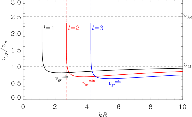
Figure 2: Dependence on the axial wavenumber $k$ of the axial group speed ($v_{\rm gr}$) of trapped coronal fast sausage modes. Derived from Figure 1a, this figure is a generalization of Figure 3b in Roberts et al. (1984).

where $v_{\rm fi}$ is the internal transverse fast speed. Equation (5) applies when $\rho_{\rm i}/\rho_{\rm e}\gg 1$, and explicitly shows that the periods of FSMs are of the order of the transverse Alfv$\acute{\rm e}$n time. Without further refinement, Equation (5) is already seismologically useful. Take the Culgoora radio spectrograph measurements of a regular series of damped pulses presented by McLean and Sheridan (1973). From Figure 2 therein one discerns a period $P\approx 4.3$ sec, and an e-fold damping time $\tau\approx 10P$. If attributing this rapid oscillation to a standing FSM of transverse order $l=1$ in a long loop, then one deduces from Equation (5) a density contrast $\rho_{\rm i}/\rho_{\rm e}\approx 100$ and a transverse fast time $R/v_{\rm fi}\approx 1.6$ sec (e.g., Kopylova et al. 2007) .

Another dispersive feature that characterizes the ER83 equilibrium is the non-monotonic frequency-dependence of the axial group speed ($v_{\rm gr}$) of trapped FSMs, as shown in Figure 2. For any transverse order, $v_{\rm gr}$ decreases from $v_{\rm Ae}$ at the cutoff to some minimum $v_{\rm gr}^{\rm min}$ before approaching $v_{\rm Ai}$ from below. Note that this figure derives directly from Figure 1, and that the non-monotonic dependence of $v_{\rm gr}$ on the axial wavenumber $k$ is equivalent to the frequency dependence because $\omega$ increases monotonically with $k$. This feature is most relevant for discussing impulsively excited FSMs, for which the perturbations like, say, the Lagrangian displacement $\xi(r,z;t)$ necessarily involve all frequencies and all wavenumbers (Roberts et al. 1984; Edwin and Roberts 1986). While initially examined by drawing analogy with the Pekeris waves in oceanography, this problem was recently placed on a firmer mathematical ground by Oliver et al. (2015). First expressing $\xi(r,z;t)$ as the Fourier integral over all $k$, this study shows that the Fourier component $\tilde{\xi}(r,k;t)$ can be expressed as (see Equation 25 therein)

$$\tilde{\xi}(r,k;t) =\sum_{l=1}^{N}\left[A_{l}^{+}(k){\mathrm{e}}^{-i\omega_{l}(k)t}+A_{l}^{-}(k){\mathrm{e}}^{i\omega_{l}(k)t}\right]\hat{\xi}_{l}(r,k)$$

$$+\int_{|k|v_{\rm Ae}}^{\infty}\left[A_{\omega}^{+}(k){\mathrm{e}}^{-i\omega(k)t}+A_{\omega}^{-}(k){\mathrm{e}}^{i\omega(k)t}\right]\hat{\xi}_{\omega}(r,k){{\rm d}}\omega~{}.$$ (6)

Here the superscripts $\pm$ pertain to forward and backward propagations in the axial direction. For a given $k$, the summation in Equation (2.1) incorporates the contribution from the $N$ discrete trapped modes with $N$ possibly zero (see Figure 1). Outside the trapped regime, the integral sees the perturbations as comprising a continuum of improper modes rather than directly the discrete leaky modes. The coefficients $A^{\pm}$ reflects how the energy contained in the initial perturbation is distributed among the trapped and continuum modes. When some signal $\phi$ is sampled along the axis and at distances sufficiently far from the exciter, trapped modes are relevant and $\phi$ goes like (Edwin and Roberts 1986, Equation 6)

$$\phi(z,t)\sim\left\{\begin{array}[]{ll}A(z,t){\mathrm{e}}^{i[kz-\omega(k)t)]}~{},{}{}{}&\omega^{\prime\prime}(k)\neq 0~{},\\ \displaystyle\frac{1}{[t|\omega^{\prime\prime\prime}(k)|]^{1/3}}{\mathrm{e}}^{i[kz-\omega(k)t)]}~{},{}{}{}&\omega^{\prime\prime}(k)=0~{}.\end{array}\right.$$ (7)

Here ${}^{\prime}\equiv{{\rm d}}/{{\rm d}k}$, and as such Equation (7) directly shows why the non-monotonic $\omega$-dependence of $v_{\rm gr}=\omega^{\prime}(k)$ matters. Note that $k$ is interpreted as dependent on $(z,t)$ through $\omega^{\prime}(k)=z/t$.

Equation (7) proves theoretically insightful and seismologically useful. At a distance $h$ from the exciter, it offers a heuristic interpretation of $\phi(h,t)$ envisaged by Roberts et al. (1984). When $h/v_{\rm Ae}<t<h/v_{\rm Ai}$, individual wavepackets with progressively low group speeds arrive consecutively, constituting the “periodic phase”. When $h/v_{\rm Ai}<t<h/v_{\rm gr}^{\rm min}$ (see Figure 2), two wavepackets with the same group speed but different frequencies arrive simultaneously, enhancing the signal in this “quasi-periodic phase”. In these phases, the situation $\omega^{\prime\prime}(k)\neq 0$ arises. When $t>h/v_{\rm gr}^{\rm min}$, no incoming wavepackets are expected, resulting in a decay phase which pertains to $\omega^{\prime\prime}(k)=0$. With a rapid pulsation measured with the Daedalus radio spectragraph, Roberts et al. (1984) illustrated how to deduce the geometrical parameters ($R$ and $h$) by combining the measurements of such timescales as the period in the decay phase and the duration of the quasi-periodic phase.

2.2 Fast Sausage Modes in ER83-like Equilibria

By “ER83-like” we mean a rather general set of equilibria that deviate from the ER83 equilibrium only slightly such that the primary dispersive properties of FSMs are preserved. The purpose is to leave more significant deviations till later, and focus here on what simplifications or complications are unlikely to cause qualitative difference to FSMs. By “primary” we list a number of dispersion features, the first two not restricted to sausage modes.

1. The dispersive properties do not depend on the direction of propagation, as ensured by the absence of an equilibrium loop flow.

2. A Fourier decomposition in the axial direction is enabled by the axial homogeneity.

3. Sausage modes can be told apart from the rest as ensured by sufficient symmetry.

4. All branches of FSMs possess cutoff wavenumbers regardless of the transverse order.

5. All branches of FSMs are characterized by a nonmonotical frequency dependence of the axial group speed in the trapped regime.

As an example, one may replace the step profile in ER83 with a configuration comprising a uniform interior, a uniform exterior, and a transition layer (TL) continuously connecting the two. In this case, Chen et al. (2016) showed that Feature 4 persists. In addition, varying $\beta_{\rm i}$ between $\sim 0$ and unity led only to a rather weak $\beta_{\rm i}$-dependence for both the cutoff wavenumbers and the eigen-frequencies at sufficiently small $k$, provided that the transverse fast time ($R/v_{\rm fi}$) is used to measure the timescales. It follows that a finite plasma $\beta$ is unlikely to alter the dispersive properties found with $\beta=0$. Indeed, the zero-$\beta$ study examining the $v_{\rm gr}-\omega$ curves indicated that Feature 5 persists, despite that multiple extrema may appear for thick TLs (Yu et al. 2016b). Seismologically, if the $\beta$-insensitivity always holds, then one is allowed to deduce the transverse Alfv$\acute{\rm e}$n time ($R/v_{\rm Ai}$) with the simpler zero-$\beta$ MHD (e.g., Nakariakov et al. 2012; Lopin and Nagorny 2014; Yu et al. 2017; Lopin and Nagorny 2019a). It is just that this deduced transverse Alfv$\acute{\rm e}$n time should be interpreted as actually being the transverse fast time.

Another school of ER83-like equilibria is realized by placing a straight, field-aligned, density-enhanced slab in an ambient corona, as first considered by Edwin and Roberts (1982). As long as the symmetry about the slab axis is maintained, the dispersive properties of FSMs are strikingly similar to the cylindrical case. Take step profiles. The cutoff wavenumber $k_{{\rm c},l}$ is identical in form to Equation (4) except that $j_{0,l}$ is replaced with $(l-1/2)\pi$ (Nakariakov and Roberts 1995a). Likewise, revising $j_{0,l}$ to $(l-1/2)\pi$ in Equation (5) yields the period $P$ for small $k$ (Chen et al. 2018a; see also Terradas et al. 2005) . In addition, both $k_{{\rm c},l}$ and the eigen-frequencies at sufficiently small $k$ are found to depend on $\beta_{\rm i}$ only weakly, for step (Inglis et al. 2009) and multi-layered profiles alike (Chen et al. 2018a). As in the cylindrical case, this $\beta$-insensitivity justifies the rather extensive use of the simpler zero-$\beta$ MHD for examining coronal FSMs (e.g., Terradas et al. 2005; Hornsey et al. 2014; Lopin and Nagorny 2015a; Yu et al. 2015; Karamimehr et al. 2019). However, we note by passing that if an equilibrium is not symmetric about the slab axis, then the sausage modes will be coupled to the kink ones, leading to a less clear distinction between the two. This asymmetry in the equilibrium arises in a number of observationally relevant situations. For instance, it appears in the presence of an external rigid boundary, which in turn appears when one addresses an external wave source (Lopin and Nagorny 2020). Likewise, it shows up when the equilibrium quantities on one side of the slab are different from those on the other side (e.g., Allcock and Erdélyi 2017; Zsámberger et al. 2018; Oxley et al. 2020).

Regarding FSMs, the similarity between the slab and cylindrical geometries enables a unified discussion on when Features 4 and 5 occur. This was done in zero-$\beta$ MHD for the equilibria where the magnetic field is uniform but the density takes a generic variation

$${\rho}(r)=\rho_{\rm e}+(\rho_{\rm i}-\rho_{\rm e})f(r)~{}.$$ (8)

Here $f(r)$ attains unity at the loop axis ($r=0$) and zero when $r\to\infty$. In the slab geometry, $r$ is interpreted as the distance ($x$) from the slab axis. In both geometries, cutoff wavenumbers exist only when $f$ decreases more rapidly than $r^{-2}$ at large distances, a concrete result obtained with Kneser’s oscillation theorem by Lopin and Nagorny (2015a) and Lopin and Nagorny (2015b). Note that $f(r)$ varies as $r^{-\infty}$ for a uniform ambient as happens for ER83. On the other hand, in general $1-f(r)$ behaves as $\propto r^{\nu}$ close to the loop axis. It was shown that the $\omega$-dependence of the axial group speed ($v_{\rm gr}$) of trapped FSMs is non-monotonic when $\nu>2$ for the cylindrical (Yu et al. 2017) and slab geometries alike (Li et al. 2018). Note that $\nu=\infty$ for step profiles as considered by ER83. Note further that such a critical $\nu$ was implied in Nakariakov and Roberts (1995b) and Lopin and Nagorny (2015b). In the former slab study, the authors examined a generalized symmetric Epstein profile $f(x)={\rm sech}^{2}[(|x|/d)^{\alpha}]$ with $d$ some mean half-width of the slab, finding that the $v_{\rm gr}-\omega$ curve is nonmonotical only when the steepness parameter $\alpha>1$. This is understandable because in this case $f(x)\approx 1-(x/d)^{2\alpha}$ for $0<x/d\ll 1$, resulting in a $\nu=2\alpha>2$ when $\alpha>1$.

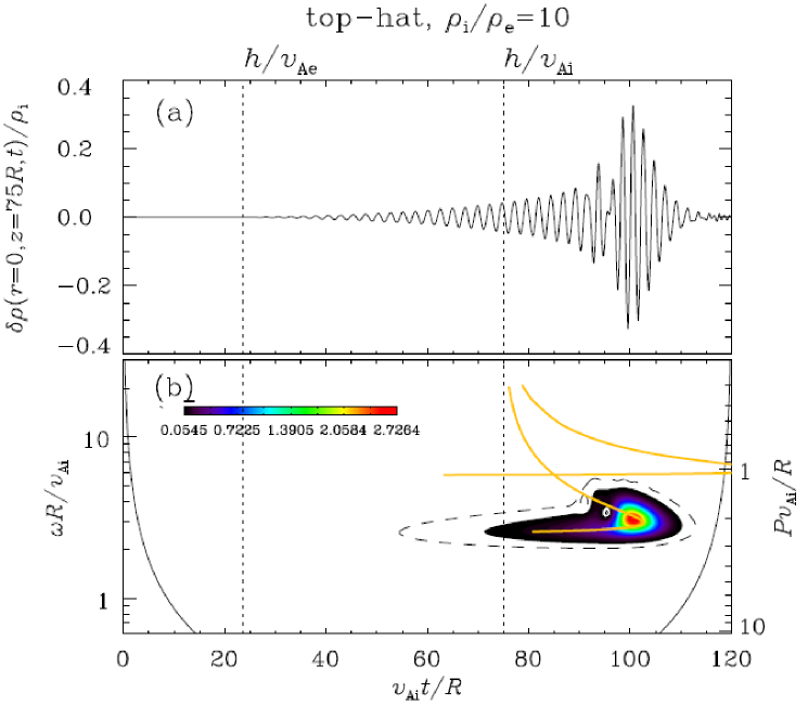
Figure 3: Signatures of an impulsively generated wavetrain sampled at a distance $h=75R$ from the exciter along the loop axis. A zero-$\beta$ version of the ER83 equilibrium is considered, with the density contrast being $\rho_{\rm i}/\rho_{\rm e}=10$. Presented are (a) the density perturbation $\delta\rho$ and (b) its Morlet spectrum. The Morlet spectrum from the time-dependent simulation is closely shaped by the yellow curve representing $\omega-h/v_{\rm gr}$ found with an independent eigenmode analysis. Taken from Yu et al. (2017) with permission.

Now we can proceed further with impulsively generated sausage wavetrains. While the physics in Equations (2.1) and (7) remains untouched, it seems more straightforward to work with the wavelet spectra of the wavetrains rather than the time series itself from the seismological perspective. This is illustrated with Figure 3, where the time series of the density variation $\delta\rho(h,t)$ and its Morlet spectrum are shown for a wavetrain sampled at a distance of $h=75~{}R$ along the axis from the impulsive localized driver. This figure was taken from Yu et al. (2017) who worked in zero-$\beta$ MHD and adopted a cylindrical geometry. Furthermore, it pertains to the simplest case where the density is piecewise constant with a density contrast $\rho_{\rm i}/\rho_{\rm e}=10$. As outlined by Roberts et al. (1984), the duration of the quasi-periodic phase proves seismologically useful. With Equation (7), this quasi-periodic phase is expected to start at $h/v_{\rm Ai}$ with the simultaneous arrivals of wavepackets with $v_{\rm gr}$ lying between $v_{\rm Ai}$ and $v_{\rm gr}^{\rm min}$. However, Figure 3a suggests that, without the vertical line marking $h/v_{\rm Ai}$, it seems difficult to tell when the quasi-periodic phase starts . While this difficulty persists in Figure 3b, the Morlet spectrum seems more informative in that it seems to be closely shaped by the yellow curves representing the wavepacket arrival time $h/v_{\rm gr}(\omega)$ as a function of $\omega$. Physically, this behavior is expected with Equation (7) given the exponential term therein. Seismologically, it should be useful if one can further localize the Morlet spectrum in the frequency direction, a point we will return to later.

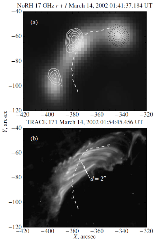
Figure 4: Structures associated with quasi-periodic pulsations (QPPs) as imaged in (a) radio and (b) EUV pertaining to an M5.7 flare on March 14 2002. Taken from Zimovets et al. (2013) with permission.

First found in a slab geometry by Nakariakov et al. (2004), the Morlet spectra similar to the one in Figure 3b are named “crazy tadpoles” given their shape. Since then crazy tadpoles have been found in multiple linear MHD computations for both cylindrical (e.g., Shestov et al. 2015) and Cartesian configurations (e.g., Pascoe et al. 2013b, 2014; Li et al. 2018) . This insensitivity to geometry is understandable because crazy tadpoles are expected as long as Features 4 and 5 persist (Yu et al. 2017). More importantly, crazy tadpoles were observed for short-period wavetrains propagating in AR loops as measured, say, during the Aug 1999 total eclipse (Katsiyannis et al. 2003, Figure 4). At this point we note that the theoretical results in wave-guiding slabs also apply when current sheets are embedded, provided that the electric resistivity vanishes (e.g., Edwin et al. 1986; Smith et al. 1997). Indeed, dispersive sausage wavetrains guided by flare current sheets have been employed to interpret some fine structures in broadband type IV radio bursts (e.g., Karlický et al. 2013; Yu et al. 2016c) .

To the list of primary dispersion features of FSMs, we need to append an item that pertains to continuous transverse profiles. This item, Feature 6 hereafter, is that an equilibrium is considered to be ER83-like if FSMs are not resonantly absorbed in the Alfv$\acute{\rm e}$n continuum, which arises when the Alfv$\acute{\rm e}$n speed profile ($v_{\rm A}$) varies continuously. Feature 6 applies to all the above-referenced equilibria despite that the axial phase speed of FSMs can indeed match $v_{\rm A}$ at some “resonant location”. Mathematically, in cylindrical geometry Soler et al. (2013) showed that this “resonant location” is not a genuine singularity that is required for an FSM to resonantly couple to the $m=0$ Alfv$\acute{\rm e}$n wave. Physically, the absence of the Alfv$\acute{\rm e}$n resonance is because the velocity ($\delta\bm{v}$) and magnetic field perturbations ($\delta\bm{B}$) associated with the Alfv$\acute{\rm e}$n waves decouple from those in FSMs (see e.g., the review by Goossens et al. 2011).

2.3 Miscellaneous

This section is devoted to the aspects that are important for coronal FSMs but not directly connected to their dispersive properties and seismological applications.

2.3.1 Excitation of Coronal Fast Sausage Waves

Coronal FSMs remain primarily invoked for interpreting short-period QPPs in flares (e.g., the review by McLaughlin et al. 2018). However, there are only a few studies that explicitly address how FSMs may result from the flaring processes. The earliest seems to be the one by McLean et al. (1971) who specifically examined what caused the regular pulses in type IV radiations measured with the Culgoora radiospectrograph on Sept 27, 1969. A coronal shock, manifested as a type II burst preceding the pulses, proved crucial. This shock was suggested to hit a pre-existing loop at low heights, exciting Alfv$\acute{\rm e}$n waves and consequently accelerating electrons that emit radio emissions. The shock then hit the loop top, exciting FSMs that then modulate the radio emissions. As such the Alfv$\acute{\rm e}$n speed in the loop was required to exceed the external one substantially. A second scenario, proposed also for pulsations in type IV radio emissions, was offered by Meerson et al. (1978). The idea is that FSMs, an eigen-oscillation of a density-enhanced loop, can be resonantly amplified by fast particles (primarily protons) trapped and bouncing in the loop. With the period given by Equation (5), the authors deduced a requirement for the speeds of the bouncing protons to reach a fraction of the light speed. A third scenario was proposed by Zaitsev and Stepanov (1982), who interpreted second-scale pulsations of flare hard X-rays by invoking FSMs in a local magnetic trap. Initially a flare loop segment close to the flaring site, this trap results when the enhanced gas pressure expands the segment. Excited by the impulsive energy release , FSMs are expected to modulate the flux of energetic electrons escaping from the trap by varying the mirror ratio. A modulation in hard X-ray fluxes then follows given that these electrons eventually hit the dense atmospheres at the loop footpoints.

Another group of scenarios for exciting FSMs largely concern AR loops. In one scenario, FSMs were observed to be generated in situ, along with kink modes, due to flow collision in a loop with coronal rain (Antolin et al. 2018). Numerical simulations provided support to this observed in-situ excitation (Pagano et al. 2019), showing that while the resulting kink modes strongly depend on the symmetry of the collision (in terms of morphology, trajectory and energy), the FSMs are to a large extent independent. Such dependency leads to mostly standing FSMs and propagating kink modes. Physically, one expects this mechanism to be common in thermally unstable loops, given that the local loss of pressure therein leads to collision of counter-streaming flows (Antolin 2020). Its occurrence is therefore tied with the amount of thermally unstable plasmas in the solar atmosphere. Observationally, however, more needs to be done to ascertain how common this excitation mechanism is, even though coronal rain is ubiquitously observed (Antolin and Rouppe van der Voort 2012). We note that the flow collision mechanism can be easily extrapolated to the flaring scenario, where the strong electron beam heating at both footpoints is expected to drive strong chromospheric evaporation, thus leading to highly energetic flow collision in the corona. This scenario is likely to be accompanied by Kelvin-Helmholtz instabilities due to shear flows, particularly in the presence of asymmetric footpoint heating (Fang et al. 2016).

FSMs in AR loops may also be connected to the footpoint motions in the lower atmosphere. This connection may be direct, as proposed by Berghmans et al. (1996) who linked coronal FSMs to axisymmetric, radial, footpoint motions due to, say, exploding granules. Alternatively, coronal FSMs may be indirectly linked to axisymmetric, azimuthal, footpoint motions, which directly drive $m=0$ Alfv$\acute{\rm e}$n waves. While propagating upward, these finite-amplitude mother waves may nonlinearly generate coronal FSMs via the ponderomotive force and nonlinear phase-mixing (Shestov et al. 2017). As demonstrated by a recent multi-instrument observational study, azimuthal motions (swirls) are indeed abundant in the photosphere, and Alfv$\acute{\rm e}$n pulses with sufficient amplitude can indeed be generated and reach at least chromospheric levels (Liu et al. 2019, and references therein).

Before proceeding, let us remark that, while physically sound, the afore-listed excitation scenarios remain largely to be tested against observations. The reason is twofold. On the one hand, candidate coronal FSMs have only been sporadically reported in the literature, making it difficult to prove or disprove a candidate excitation scenario in the statistical sense. On the other hand, a substantial fraction of the excitation scenarios have yet to be made more quantitative to come up with a list of tell-tale observational signatures. This in turn involves two steps. Firstly, one needs to invoke one specific scenario to predict, say, the characteristic periodicities and variations in such primitive quantities as the magnetic field. Secondly, one needs to translate the predicted variations in the primitive physical variables into measurables. Both steps are subject to substantial intricacies, with those in the second step detailed in Section 3.

2.3.2 Damping

Being highly compressible, FSMs are likely to be damped by non-ideal effects like radiative loss, electron thermal conduction, and proton viscosity. Usually the damping due to radiative loss can be neglected, at least for ER83-like equilibria . However, in general the importance of the rest of the non-ideal mechanisms depends sensitively on the equilibrium parameters (e.g., Kopylova et al. 2007). The consequence is twofold. One, an assessment of the damping rates can usually be done only a posteriori, given that many equilibrium parameters are not known before the seismological practice. Two, the assessment in general needs to be conducted on a case-by-case basis, given the diversity of the equilibrium parameters. Examining the McLean and Sheridan (1973) event, Kopylova et al. (2007) concluded that non-ideal effects are orders-of-magnitude weaker than the damping due to lateral leakage.

Lateral leakage, manifested by the non-zero $\omega_{\rm I}$, is an ideal process whereby oscillating loops lose their energy by continuously emitting fast waves into the ambient. With this picture established decades ago (Zajtsev and Stepanov 1975; Spruit 1982), it suffices to highlight the importance of examining leaky FSMs from an initial-value-problem (IVP) rather than an eigen-value-problem (EVP) perspective. The problem is, the eigen solutions to the EVP problem increase indefinitely with distance in the exterior, making its physical reality apparently questionable. However, this reality can be recognized in two ways, both pertaining to the temporal evolution of the loop system (Cally 1986). If a continuous energy supply is available, then a steady state can be maintained where the system oscillates at the eigen-period but experiences no damping. If the waves are excited by an initial “kick”, then outgoing fast waves result in the exterior, the amplitude increasing with distance behind the wave front at a given instant but diminishing with time at a given location. Both expectations have been extensively seen in time-dependent computations for loops experiencing kicks (e.g., Terradas et al. 2005, 2007; Nakariakov et al. 2012). In particular, the periods and damping times agree with the eigen-frequencies, provided that an FSM with a particular transverse order $l$ is primarily excited. This is true for both $l=1$ (e.g., Guo et al. 2016) and higher $l$ (Lim et al. 2020). The EVP approach can therefore be seen as a shortcut given that it is usually much less computationally expensive than the IVP approach. Physically, with the system evolution in general expressible by Equation (2.1), Oliver et al. (2015) proposed that the outgoing waves result from the interference of the continuum modes. The agreement in the periods and damping times between the EVP and IVP approaches is therefore likely to result from this interference as well, with the assertion regarding the period explicitly demonstrated by Andries and Goossens (2007).

2.3.3 Multi-stranded vs. Monolithic Loops

In principle, an unambiguous definition of sausage modes is ensured only by the sufficient symmetry of the equilibria. With Figure 4, taken from Zimovets et al. (2013), we show that in some spatially resolved measurements of QPPs in flares, what appears as an isolated loop in moderate-resolution images (acquired with, say, NoRH, Figure 4a) may be further resolved into a multitude of fine strands in high-resolution images (observed with, e.g., TRACE, Figure 4b). Such a system does not seem to possess sufficient symmetry, and a theoretical study explicitly addressing the existence of sausage modes in similar systems has yet to appear. Nonetheless, some IVP studies on FSMs in coronal loops with fine structures in the form of concentric shells indicated that the periods (Pascoe et al. 2007) and damping times (Chen et al. 2015a) are consistent with the values found with monolithic loops, provided that the number of shells exceeds, say, $\sim 10$. This insensitivity to fine-structuring is not an answer to the question at hand because of the symmetry of the adopted equilibria. However, the hint is that sausage-like modes are expected if the spatial scales of the initial perturbations considerably exceed those associated with fine structures. By “sausage-like” we mean the modes characterized by coherent breathing motions of a collection of strands as happens for an ER83-like loop experiencing sausage modes. In fact, this intuitive expectation has been practiced in a considerable number of observational studies on sausage modes in the lower solar atmosphere (e.g., Dorotovič et al. 2008; Morton et al. 2012; Grant et al. 2015), despite the irregularity of the shape of the examined structure and the fine-structuring therein (e.g., Keys et al. 2018, Figure 4a).

2.3.4 Loop Curvature

As envisaged by Roberts (2000), the distinction between sausage and kink modes will be less clear in curved than in straight tubes, one reason being that kink modes will lead to the breathing motions that characterize sausage modes. A substantial number of theoretical studies on collective waves in curved loops then followed, the focus nonetheless being kink modes (see the review by Van Doorsselaere et al. 2009, and further studies, e.g., Ruderman 2009, Selwa et al. 2011, and Magyar and Nakariakov 2020). The studies explicitly addressing FSMs pertain exclusively to curved slabs in a zero-$\beta$ equilibrium either directly described by  (e.g., Verwichte et al. 2006a, b; Díaz et al. 2006) or similar to (e.g., Díaz 2006; Hindman and Jain 2015; Thackray and Jain 2017) the following configuration. A cylindrical geometry $(\bar{r},\bar{\phi},\bar{z})$ is involved, the corresponding Cartesian system being $(\bar{x},\bar{y},\bar{z})$. The equilibrium magnetic field $\bm{B}_{0}$ is purely in the $\bar{\phi}$-direction, its strength $\propto 1/\bar{r}$. With the plane $\bar{y}=0$ representing the dense photosphere, all field lines form line-tied semi-circles. The mass density depends only on $\bar{r}$ as $\propto\bar{r}^{\alpha}$ with $\alpha$ being a constant. The constant of proportion in the region $|\bar{r}-\bar{r}_{0}|\leq R$ is different from the rest, thereby outlining a density-enhanced curved slab with length $L=\pi\bar{r}_{0}$ and semi-width $R$. For waves propagating only in the $\bar{x}-\bar{y}$ plane, the velocity perturbation is in the $\bar{r}$-direction only. The $\bar{\phi}$-independence of the equilibrium parameters and the line-tied boundary condition further dictate that the Fourier amplitude of this perturbation is $\propto\tilde{v}(\bar{r})\sin(\bar{m}\bar{\phi})$, with $\bar{m}=1,2,\cdots$ being the axial harmonic number. As outlined by Verwichte et al. (2006a) and Díaz et al. (2006), the distinction between sausage and kink modes relies on the inspection of the spatial profile of $\tilde{v}(\bar{r})$, the modes with breathing motions being classified as sausage modes. Furthermore, whether modes are leaky depends on the sign of $\mu_{\rm e}^{2}$ defined in Equation (3), with $k$ now $\bar{r}$-dependent because of the $\bar{r}$-dependence of the length of field lines. Verwichte et al. (2006a) showed that the modes leak towards large (small) $\bar{r}$ when $\alpha>-4$ ($\alpha<-4$). In the particular case where $\alpha=-4$, trapped modes arise when the phase speed is below the Alfv$\acute{\rm e}$n speed profile (see Figure 2 therein).

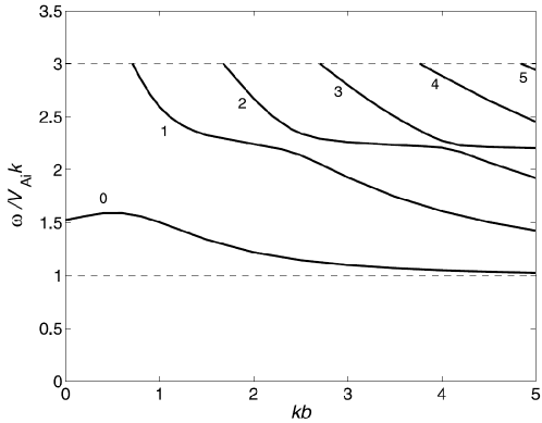
Figure 7: Dependence on the axial wavenumber $k$ of the axial phase speed ($\omega/k$) for fast sausage modes in a zero-$\beta$ cylindrical equilibrium. The equilibrium magnetic field $\bm{B}_{0}$ is uniform and axially directed in the regions $r<b$ and $r>a$, whereas $\bm{B}_{0}$ is purely azimuthal in the annulus $a<r<b$. The mass density is distributed in a such a way that the Alfv$\acute{\rm e}$n speed determined by $\bm{B}_{0}$ is piece-wise constant across $r=b$. Note that the transverse fundamental is trapped regardless of $k$. Taken from Khongorova et al. (2012) with permission.

Of interest is how well the theoretical results on FSMs in straight slabs apply. When $\alpha=-4$, a remarkable one-to-one correspondence between the curved and straight cases is seen, and the difference in the eigen-frequencies is discernible only when $L/R$ is unrealistically small (Verwichte et al. 2006a, Figures 4 and 11). On the contrary, the eigen-frequencies agree with the straight-slab results only for sufficiently small $L/R$ when $\alpha=0$, corresponding to a piece-wise constant transverse profile for the density. For this agreement to happen, however, $L/R$ does not need to be unrealistically small (Díaz et al. 2006, Figure 7). In addition, while sausage modes are indeed always leaky in this case, the damping rate can be sufficiently weak to ensure observability for sufficiently large density contrasts (Figure 8 therein). The same happens also for the FSMs examined in the study by Pascoe and Nakariakov (2016), where the equilibrium essentially pertains to the situation where $\alpha=-2$, corresponding to a piece-wise constant transverse profile for the Alfv$\acute{\rm e}$n speed. In this case, the periods of FSMs differ from the straight-slab expectations by no more than $\sim 7.5\%$ for an $L/R$ of $8.3$ and a density contrast of $50$, both values being reasonable for flare loops .

2.3.5 Energy Propagation in Sausage Modes

Given the prominence of the coronal heating problem in solar and astrophysics, one naturally asks how much energy is propagated in sausage modes (see also the review by Van Doorsselaere et al., this issue). This is particularly relevant for the lower solar atmosphere, where sausage modes have been observed to be sufficiently energetic in a considerable number of structures of various sizes, with sunspots (Dorotovič et al. 2014), pores (Grant et al. 2015), mottles (Morton et al. 2012), and chromospheric brightenings associated with plages/enhanced-network regions (Guevara Gómez et al. 2020) being examples. Theoretical examinations were therefore performed for sausage modes from the energetics perspective with photospheric and/or chromospheric applications in mind. However, they are expected to readily find applications to future high-resolution observations of sausage modes in the higher corona. Indeed, for FSMs that are in-situ generated through flow collision, the observed amplitudes can reach up to $\sim 40~{}{\rm km}~{}{\rm s}^{-1}$ for cool an dense coronal rain flows, leading to energy flux densities on the order of $10^{7}-10^{8}$ erg cm^-2 s^-1 (Antolin et al. 2018). The energy flux densities remain substantial for more “typical” coronal conditions, despite that they are roughly $2-3$ orders of magnitude lower in this case.

To calculate the energy in sausage modes, Moreels et al. (2015) used the theory that was worked out for kink modes by Goossens et al. (2013). They computed the kinetic and magnetic energy in the ER83 model with zero plasma-$\beta$. Moreels et al. (2015) additionally assumed $m=0$ symmetry and also extended the theory to non-zero plasma-$\beta$, and incorporated internal energy as well. However, the latter was not important for the energy flux in FSMs, because their energy flux is entirely in the Poynting flux $\langle\overline{\mbox{$\bm{S}$}}\rangle$. For FSMs with frequency near the cut-off frequency, the energy flux is purely in the magnetic field direction and is given by

$$\langle\overline{\mbox{$\bm{S}$}}\rangle=2\frac{\rho_{\rm i}k^{2}v_{\rm Ai}^{2}+\rho_{\rm e}k^{2}v_{\rm Ae}^{2}\ln(1/f)}{4}v_{\rm Ae}\pi R^{2}\Xi_{r}^{2}\hat{z},$$ (9)

where $\Xi_{r}$ is the maximal radial displacement at the loop boundary. In this equation $f$ plays the role of filling factor: it measures the fractional surface of density enhanced flux tubes in a cross-section of a bundle of loops (for more information and explanation, see Van Doorsselaere et al. 2014). By considering the limits $f\to 0$ (a single loop), this equation shows that the exterior part is causing troubles because of the leaky nature of FSMs. Indeed, in that limit, the Hankel functions in the exterior will not be square-integrable and lead to infinite energy. For completeness, the expressions for energy propagation in the SSMs in the long-wavelength limit is given by

$$\langle\overline{\mbox{$\bm{T}$}}\rangle=\frac{\rho_{\rm i}}{2}k^{2}c_{\rm Ti}^{2}\pi R^{2}\Xi_{z}^{2}c_{\rm Ti}\hat{z},$$ (10)

where $\Xi_{z}$ is now the longitudinal component of the displacement at the loop boundary. The energy flux is only in the internal energy flux, is only inside the loop (and thus only determined by interior loop parameters), and is once again purely along the magnetic field. For more general expressions and more detailed explanations for their derivations, see Moreels et al. (2015). These formulae were successfully used to observationally determine the energy content of sausage waves in e.g. Grant et al. (2015); Keys et al. (2018); Gilchrist-Millar et al. (2020).

3 Forward Modeling of Coronal Fast Sausage Modes

The fluid and magnetic parameters from analytical and numerical studies on coronal FSMs usually do not translate into observables in a straightforward manner, thereby necessitating proper forward modeling (see also the review by Anfinogentov et al. in this issue for forward modeling studies on other modes). This can be illustrated with the intensity ($I$) of emission lines in, say, (E)UV for which the corona is optically thin (e.g., Del Zanna and Mason 2018),

$$I=\int_{\rm LoS}\frac{\epsilon}{4\pi}ds~{}.$$ (11)

Here $s$ is the coordinate along the line of sight (LoS), and by integration $I$ collects all photons emitted from a square of size $\Delta_{\rm pixel}$ when projected onto the plane of sky (PoS). Furthermore, the emissivity $\epsilon$ is given by $N^{2}G_{\lambda 0}$ with $N$ being the electron density and $G_{\lambda 0}$ the contribution function for an emission line centered at $\lambda_{0}$ in rest frame. Substantial atomic physics is involved in $G_{\lambda 0}$, where all terms depend essentially only on the electron temperature $T$ with the possible exception of the ionic fraction ($f_{q}$) of the line-emitting ions (e.g., Shi et al. 2019c, Equation 23). In equilibrium ionization (EI), this $f_{q}$ is essentially only $T$-dependent as well, making $G_{\lambda 0}$ dependent only on $T$. Taking advantage of the simplicity of EI, Gruszecki et al. (2012, also the references therein) were the first to recognize the instrument-sensitivity of the detectability of FSMs by further assuming the $T$-profile to be uniform along an LoS. The result is that, if the pixel size $\Delta_{\rm pixel}$ substantially exceeds the loop width, then the leading-order density perturbations do not survive the LoS integration (Figure 4 therein), thereby making the detection of FSMs unlikely. Physically, this was attributed to that FSMs displace fluid parcels primarily in the transverse direction in a low-$\beta$ equilibrium but mass conservation is always maintained.

3.1 Thermal Emissions

Forward models that examine the modulation of thermal emissions by FSMs have been conducted only for emission lines in the (E)UV and only for ER83-like equilibria. A notable step forward was made by Antolin and Van Doorsselaere (2013, AVD13), who incorporated $G_{\lambda 0}$ in the examinations on how trapped FSMs modulate the Fe IX 171 Å and Fe XII 193 Å emissions detected with both imaging and spectroscopic instruments. The spatial profiles of the fluid parameters were essentially a three-dimensional representation of the eigen-solutions in an ER83 equilibrium. AVD13 noted that, unlike for photospheric conditions, the variation in the loop radius produced by the FSM tends to be $\lesssim 25$ km for typical coronal conditions (this results from the strong compressibility of FSMs, see e.g., Equation 10 in Yu et al. 2016a). The detectability of FSMs was shown by AVD13 to depend sensitively on such geometrical parameters as viewing angles of the LoS, and, in particular, on the temporal and spatial resolutions of the instrument. The issue with temporal cadence arises from the short period of FSMs, which led AVD13 to propose that the ionic fractions ($f_{q}$) may not respond instantaneously to the temperature variations to maintain ionization equilibrium. Indeed, it was shown by Shi et al. (2019a) that non-equilibrium ionization (non-EI) effects are negligible only when the angular frequencies $\omega$ of FSMs are far below the ionization and recombination frequencies ($\nu_{\rm C}$ and $\nu_{\rm R}$). This requirement is more stringent than that the wave period $P=2\pi/\omega$ be much longer than the ionization and recombination timescales ($1/\nu_{\rm C}$ and $1/\nu_{\rm R}$). Non-EI effects are therefore seen even in the study on the Fe XXI 1354 Å line emitted from flare loops, despite the high densities therein (Shi et al. 2019a). That said, the non-EI computations differ from their EI counterparts only in intensity variations, whereas the Doppler shifts and Doppler widths hardly experience any influence. Indeed, AVD13 showed that the wave modulation of spectroscopic quantities is substantial, particularly for the Doppler width.

Summing up AVD13, Shi et al. (2019c) and Shi et al. (2019a), one expects the following (E)UV signatures of fundamental trapped FSMs. Firstly, the intensity variations consistently possess the same period as the FSM. Secondly, the same is true for the variations in the Doppler shift, which nonetheless can be seen only when the loop is sampled at non-$90^{\circ}$ angles with respect to its axis. In general, a non-$90^{\circ}$ phase-difference exists between the intensity and Doppler shift profiles, with the deviation from the $90^{\circ}$ expectation from non-EI effects. Thirdly, in general the variations in the Doppler width possess two periodicities, one at the wave period ($P$) and the other at $P/2$. This behavior results from the competition between the broadening due to bulk flow (the $P/2$-periodicity) and that due to temperature variations (the $P$-periodicity), meaning that the relative importance of the two periodicities may be considerably different for different emission lines. For non-flaring conditions, the effect due to bulk flow perturbations dominates over that due to fluctuating thermal motions, leading to a dominant $P/2$-periodicity. The opposite happens for flaring conditions, resulting in a dominant $P$-periodicity. These signatures are in close agreement with the IRIS flare line Fe XXI 1354 Å observations reported by Tian et al. (2016), with some indication of the weaker $P/2$-periodicity discernible in Figure 4 therein despite the cadence issue. This agreement lends some concrete support to the interpretation of this IRIS observation in terms of a fundamental FSM (also see Table 2 in Antolin and Van Doorsselaere (2013) and Fig. 15 in Hinode Review Team et al. (2019) for a summarizing diagram of observables in non-flaring conditions).

The detailed signatures aside, the point to draw from this series of forward modeling studies on fundamental FSMs is that the spectroscopic variations are in general detectable when coronal loops are not too poorly resolved spatially. For fundamental FSMs, the periodicity found from the intensity variations faithfully reflects the wave period for trapped and leaky modes alike. This latter point was shown by Shi et al. (2019b), who also demonstrated that the damping time derived from the intensity variations can largely reflect the wave damping time if the loop temperature is not drastically different from the nominal line formation temperatures expected with equilibrium ionization.

3.2 Non-Thermal Emissions

QPPs are frequently detected in radio and microwave emissions of solar flares. However, telling their physical cause(s) and hence their connections to FSMs is non-trivial. Basically, all radio emission mechanisms can be divided into incoherent (say, gyrosynchrotron, free-free) and coherent (maser and plasma) ones, and interpreting and modeling the QPPs in radio bursts produced by different mechanisms require different approaches. As a rule, the incoherent gyrosynchrotron mechanism is responsible for the so-called microwave flaring continuum, while the coherent plasma mechanism is believed to produce the decimetric and metric radio bursts, including both the broadband continuum and various fine temporal and spectral structures in these ranges.

3.2.1 Gyrosynchrotron Microwave Emissions

In the microwave range ($\sim 3-100$ GHz), the nonthermal flare emissions are produced mainly by the incoherent gyrosynchrotron mechanism (Melrose 1968; Ramaty 1969). This mechanism is highly sensitive to the parameters characterizing the magnetic field, energetic electrons, and thermal plasmas. As such, the observed QPPs can result from both direct modulations of the emission source parameters by MHD waves and quasi-periodic injections of energetic electrons. Since the basic characteristics of QPPs, the periods for instance, can be interpreted in multiple ways, identifying their origin requires looking for more subtle features (e.g., relations between the pulsations in different spectral channels) and comparing observations with simulations. In particular, a typical solar microwave gyrosynchrotron spectrum peaks at around $\sim 10$ GHz and consists of both optically thick (below the peak frequency) and optically thin (above the peak frequency) parts, thereby implying different dependencies on the source parameters and hence, possibly, different oscillation patterns. In a sufficiently dense plasma, the spectral shape can be additionally affected by the so-called Razin effect, which suppresses the gyrosynchrotron emission at low frequencies.

Relatively simple models were adopted in the first simulations of gyrosynchrotron microwave emissions from oscillating flaring loops (Kopylova et al. 2002; Nakariakov and Melnikov 2006; Reznikova et al. 2007; Fleishman et al. 2008; Mossessian and Fleishman 2012). By simple, we mean that the simulations largely assumed a homogeneous emission source, neglected the spatial structures of the oscillations, and retained only the temporal variations of the source parameters that are typical of the considered MHD mode. Despite this, when invoking standing FSMs, this approach was able to capture the essential consequences of the oscillating axial magnetic field ($B_{\parallel}$), the defining characteristic of FSMs. For instance, concentrations of thermal and nonthermal electrons were allowed to depend on the time-varying $B_{\parallel}$. Likewise, the energies of non-thermal particles were allowed to fluctuate as happens in a time-varying magnetic trap (Mossessian and Fleishman 2012). As an exemplary result from the first simulations, the commonly observed coherent behavior of microwave QPPs in a wide range of frequencies were interpreted as an indication of high plasma densities in flaring loops, when the gyrosynchrotron emission is strongly affected by the Razin effect.

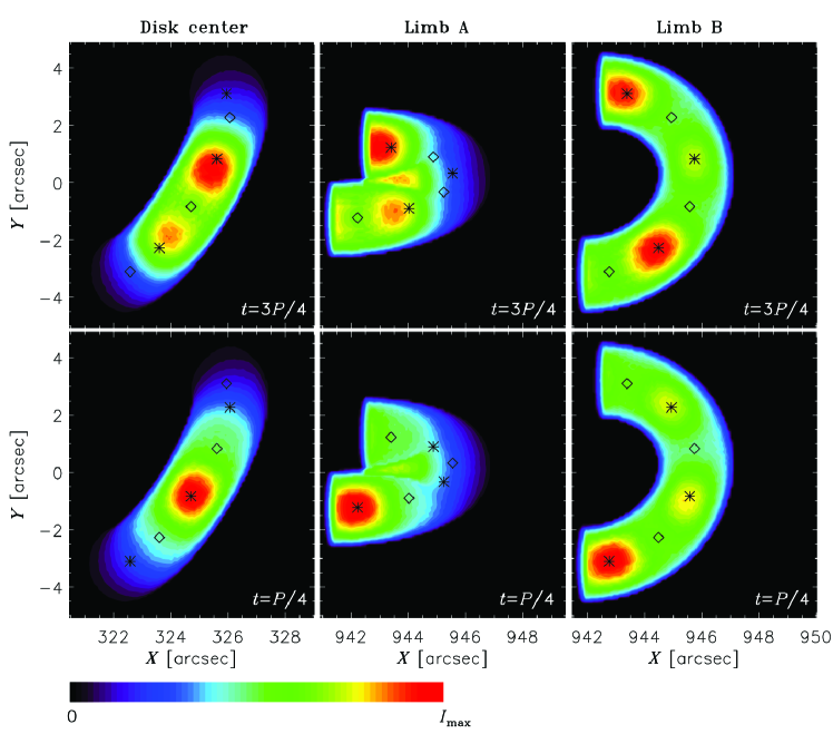
Figure 5: Two-dimensional maps of the microwave emission from a curved loop containing three standing sausage waves, for three different loop orientations and two oscillation phases. The asterisks ($\ast$) and diamonds ($\diamond$) mark the points with the maximum / minimum magnetic field at the loop axis, respectively.. Taken from Kuznetsov et al. (2015) with permission.

Later simulations, however, have revealed that the spatial structures of MHD waves need to be taken into account. Reznikova et al. (2014, 2015) and Kuznetsov et al. (2015) adopted the well-known ER83 model of MHD oscillations in an over-dense cylinder, thereby accounting for the parameter variations both along and across the cylinder, and incorporating both the axial and radial components of the magnetic field. The concentration of nonthermal electrons inside the cylinder was assumed to be proportional to the thermal plasma density . With this source model, computing the gyrosynchrotron emission required a full 3D approach, for which purpose the Fast Gyrosynchrotron Codes (Fleishman and Kuznetsov 2010) were used. Reznikova et al. (2014, 2015) considered a straight cylinder, which could be observed from different angles. Kuznetsov et al. (2015) considered a curved semi-circular loop (see Figure 5) where the viewing angle varies continuously along the loop. The following main results have been obtained:

• If the thermal plasma density is relatively low such that the Razin effect is negligible, then the high-frequency (optically thin) and low-frequency (optically thick) emissions oscillate in phase. An exception occurs in a relatively narrow band just below the spectral peak, and the oscillations therein are shifted by roughly a quarter of an MHD wavelength with respect to those at higher and lower frequencies.

• If the thermal plasma density is high, then the emission spectrum can be dominated by the Razin effect. In this case, the emissions across almost the entire spectrum oscillate in phase. An exception occurs at the lowest frequencies (much lower than the spectral peak). The oscillation phase therein reverses, and the reversal frequency depends on the viewing angle.

• The modulation depth of microwave oscillations is higher in the optically thin frequency range, reaching a few tens percent for reasonable parameters of nonthermal particles and MHD waves.

• In all cases and at all frequencies, the emission polarization (the absolute value of Stokes $V$) oscillates in phase with the intensity (Stokes $I$).

• Averaging over the visible source area (for both the optically thick and thin emissions) or along the line of sight (for the optically thin emission) reduces the amplitudes of the microwave oscillations, which limits our ability to detect and interpret them.

In solar flares, the observed microwave QPPs are usually broadband, meaning that the pulsations are synchronous at all frequencies including the optically thin and thick ranges (e.g., Reznikova et al. 2007; Fleishman et al. 2008; Inglis et al. 2008; Mossessian and Fleishman 2012). According to the above-referenced simulations, such a behavior is well consistent with the modulation of the emission by FSMs for a broad range of parameters (both low and high plasma densities). However, the same pattern is also expected for the quasi-periodic injection of energetic particles. It then follows that a reliable identification of the physical causes of QPPs requires using observations in other spectral ranges (X-ray and EUV, to name but two) and/or imaging spectroscopy microwave observations with sufficient spatial and spectral resolutions.

3.2.2 Oscillations in Zebra Patterns

Zebra patterns are an intriguing type of fine structures in the dynamic spectra of solar radio emissions observed in metric, decimetric and microwave ranges. They appear as sets of nearly parallel bright and dark stripes superimposed on broadband type IV bursts. The most common interpretation links the formation of zebra patterns to the so-called double resonance effect (Zheleznyakov and Zlotnik 1975; Kuznetsov and Tsap 2007). According to this model, individual zebra stripes are formed at the locations where the specific resonance condition is satisfied:

$$f_{\mathrm{uh}}=\sqrt{f_{\mathrm{pe}}^{2}+f_{\mathrm{ce}}^{2}}\simeq sf_{\mathrm{ce}},$$ (12)

where $f_{\mathrm{pe}}$, $f_{\mathrm{ce}}$ and $f_{\mathrm{uh}}$ are the electron plasma frequency, electron cyclotron frequency and upper-hybrid frequency, respectively. Furthermore, $s$ is an integer cyclotron harmonic number (usually $s\gg 1$). The radio emission itself is produced at the upper-hybrid frequency or its second harmonic, due to the nonlinear transformation of plasma waves excited by nonthermal electrons with a loss-cone distribution. In an inhomogeneous coronal magnetic loop (where the ratio $f_{\mathrm{pe}}/f_{\mathrm{ce}}$ is variable), condition (12) is satisfied at different heights for different harmonic numbers, which results in the formation of the characteristic striped spectrum. Since an MHD oscillation affects the local values of the magnetic field and/or plasma density (and hence $f_{\mathrm{ce}}$ and/or $f_{\mathrm{pe}}$), the locations of the double plasma resonance layers are changed accordingly, which should result in periodic oscillations (“wiggles”) of the zebra stripes. These wiggles were indeed observed in many events (e.g., Yu et al. 2013; Kaneda et al. 2018; Karlický and Yasnov 2020). The observed periods of oscillations ($\sim 0.5-2$ s) are consistent with the periods of FSMs, and the amplitude of wiggles ($\Delta f/f\sim 1-2\%$) implies a relatively low amplitude of the modulating MHD waves.

Yu et al. (2016c) simulated the modulation of zebra stripes by fast sausage oscillations. The emission source (in the equilibrium state) was modeled by a straight field-aligned overdense plasma slab (Edwin and Roberts 1982) with a constant magnetic field but gradually varying (along the slab) plasma density. After an initial perturbation, the evolution of the plasma and magnetic field parameters was simulated numerically using the Lare2D code (Arber et al. 2001). Both standing and propagating fast magnetoacoustic waves were considered. The time-dependent locations of the double plasma resonance layers and corresponding emission frequencies were computed assuming that the emission occurs at the slab axis. The simulations demonstrated that the MHD waves (with the fluctuation amplitudes of $\Delta B/B_{0}\sim 0.01-0.02$ and $\Delta\rho/\rho_{0}\sim 0.02-0.04$) are able to produce wiggles similar to the observed ones. Furthermore, standing MHD waves produce synchronous wiggles in adjacent zebra stripes, while a propagating wave leads to a delay (phase shift) between the wiggles in different stripes.

Yu et al. (2013) concluded that the quasi-periodic wiggles of the zebra pattern observed on 2006 December 13 were caused by a standing sausage oscillation. In contrast, Kaneda et al. (2018) found that the quasi-periodic oscillations in the 2011 June 21 event can be interpreted in terms of fast sausage waves propagating upward with speeds of $3000-8000$ km $\textrm{s}^{-1}$. Using observations of wiggles in the zebra pattern on 1999 February 14, Karlický and Yasnov (2020) estimated the levels of magnetic field and plasma density turbulence as $\sim 10^{-3}-10^{-2}$, and found indications that the turbulence was anisotropic. The magnetic field and plasma density in this event oscillated in phase, thus favoring fast waves.

3.2.3 Fiber Bursts

Fiber bursts (or intermediate drift bursts) are another type of fine spectral structures superimposed on the broadband type IV radio bursts (e.g., Bernold and Treumann 1983; Benz and Mann 1998). They appear in dynamic radio spectra as narrowband frequency-drifting features, often exhibit a weaker absorption stripe adjacent to the main emission stripe, and usually occur in large groups (clusters). Two features are particularly noteworthy. Firstly, the characteristic frequency drift rates of fiber bursts are intermediate between those of type II and type III bursts. Secondly, the quasi-periodic time structure of fiber clusters sometimes leads to the characteristic tadpole features in the wavelet spectra at a single frequency (e.g., Mészárosová et al. 2011; Karlický et al. 2013). These features have prompted an interpretation that fiber bursts are produced due to the modulation of the background type IV emission by propagating fast magnetoacoustic wavetrains (Kuznetsov 2006; Mészárosová et al. 2011; Karlický et al. 2013). On the other hand, the emission itself is believed to be produced by trapped nonthermal electrons with a loss-cone distribution, via the plasma emission mechanism.

Kuznetsov (2006) performed numerical simulations of the dynamic radio spectra modulated by a single propagating MHD disturbance superimposed on the large-scale (decreasing with height) profiles of the plasma density and magnetic field. The small-scale plasma density and magnetic field perturbations were assumed to vary in anti-phase. The emission was assumed to be produced at the second harmonic of the local upper-hybrid frequency $f_{\mathrm{uh}}$. The radio spectrum was affected firstly by the redistribution of the emission over frequency due to variations of the local upper-hybrid frequency caused by the MHD disturbance. Secondly, a local decrease of the magnetic field gradient in the MHD disturbance was assumed to increase the efficiency of the loss-cone instability and hence to increase the emission intensity in the corresponding region. Overall, the simulations demonstrated that MHD disturbances with propagation speeds of a few thousand ${\rm km}~{}{\rm s}^{-1}$, spatial scales of a few hundred km, and amplitudes of $\Delta\rho/\rho_{0}\sim 10^{-3}-10^{-2}$ are able to produce fiber bursts with observed parameters, including the frequency drifts, spectra and time profiles.

Karlický et al. (2013) performed similar simulations, but considered fast magnetoacoustic wavetrains consisting of multiple pulses. In contrast to the model of Kuznetsov (2006), the plasma density and magnetic field in the MHD waves were assumed to oscillate in phase, which is more adequate for the fast sausage waves. On the other hand, possible modulation of the plasma emission mechanism by the MHD wave was neglected and only the emission redistribution due to the varying upper-hybrid frequency was considered. Again, the simulations (for waves with propagation speeds of $\sim 1000~{}{\rm km}~{}{\rm s}^{-1}$, wavelengths of $\sim 200$ km, and amplitudes of $\Delta\rho/\rho_{0}=\Delta B/B_{0}=0.01$) produced the dynamic spectra with the fiber bursts (and burst clusters) very similar to the observed ones. Karlický et al. (2013) also performed numerical MHD simulations of a fast magnetoacoustic wavetrain propagating along a vertical current sheet, which allowed to reproduce the complicated time-frequency behavior (with variable frequency drifts) sometimes observed in the dynamic spectra of fiber bursts.

3.2.4 Quasi-periodic Structures in Type IIIb Bursts

Solar type III radio bursts often appear to comprise multiple narrowband slowly-drifting substructures (“striae”). Such events are sometimes called type IIIb bursts. Type III bursts are produced by relativistic electron beams propagating along open magnetic field lines, and the striae are believed to occur due to the modulation of the emission mechanism by small-scale inhomogeneities of plasma density. In other words, the radio spectrum provides an instant snapshot of the structure of the inhomogeneities. Recently, one such burst (on 2015 April 16) was observed with unprecedented spectral and temporal resolution with the Low Frequency Array (LOFAR) in the 30-80 MHz frequency range, with the fine spectral structures studied in detail by Kontar et al. (2017); Chen et al. (2018b); Kolotkov et al. (2018); Sharykin et al. (2018). In particular, Kolotkov et al. (2018) have detected quasi-periodic behavior in the frequency profile of the burst, which suggests the presence of propagating MHD waves.

Kolotkov et al. (2018) performed numerical simulations of the dynamic radio spectra, in application to the mentioned event. The emission was assumed to be produced at the local plasma frequency, and the intensity variations were caused by the redistribution of the emission over frequency due to the fluctuations of the local plasma density. The source model included the large-scale background profile of the plasma density (described by the Newkirk formula) perturbed by two propagating harmonic waves with variable wavelengths, phases, speeds and amplitudes. Comparison of the simulations with the observations (using the MCMC method) revealed two quasi-oscillatory components: the shorter one with a wavelength of $\sim 2$ Mm, speed of $\sim 657$ km $\textrm{s}^{-1}$ (which implies an oscillation period of $\sim 3$ s) and a relative amplitude of $\Delta n/n_{0}\sim 0.35\%$, and the longer one with a wavelength of $\sim 12$ Mm and relative amplitude of $\sim 5.1\%$ (the speed was not reliably determined). These wave parameters are consistent with properties of fast magnetoacoustic wavetrains.

4 Coronal Fast Sausage Modes with non-ER83-like Dispersion Features

This section is devoted to non-ER83-like equilbria, by which we mean that the FSMs hosted therein do not inherit the entire list of primary dispersion features in section 2.2. As such, this section is ordered largely in accordance with that list, and effort is taken to make different subsections as mutually exclusive as possible.

4.1 Coronal Loops with Axial Flows

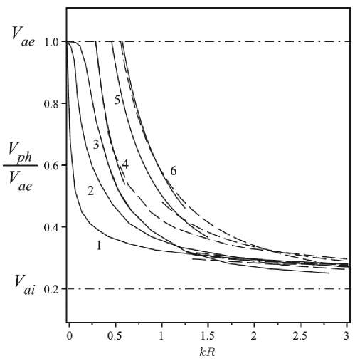
Figure 6: Dependence on the axial wavenumber $k$ of the axial phase speed ($v_{\rm ph}$) for fast sausage modes in a zero-$\beta$ cylindrical equilibrium. The equilibrium magnetic field is uniform, and a continuous density profile is realized with $f(r)$ as in Equation (8). Curves 1 to 3 pertain to an $f(r)$ of $1/[1+(r/R)^{\alpha}]$ with $\alpha=1/2,1,3/2$. Curves 4 to 6 pertain to an $f(r)$ of $\exp[-(r/R)^{\alpha}]$ with $\alpha=1,2,50$. The density contrast $\rho_{\rm i}/\rho_{\rm e}=25$, and only transverse fundamentals are considered. Cutoff wavenumbers are present in curves 4 to 6 but absent in curves 1 to 3. Taken from Lopin and Nagorny (2015b) with permission.

For loops without equilibrium flow ($\bm{v}_{0}$), one is allowed to examine only a quadrant of the $\omega-k$ plane to examine the dispersive properties of coronal FSMs. Such a symmetry is lost when $\bm{v}_{0}$ does not vanish, thereby violating Feature 1 (see the appendix of Li et al. 2013 for an illustration, also the introduction therein for early studies addressing non-zero $\bm{v}_{0}$). Focusing on coronal FSMs, the available studies seem to pertain exclusively to a time-independent field-aligned flow in straight loops, although the transverse profiles were allowed to be either step (e.g., Yu et al. 2016a) or continuous (e.g., Li et al. 2014). Of interest were standing modes in loops of length $L$, for which the axial wavenumbers ($k^{+}$ and $k^{-}$) of the component running waves need to satisfy $k^{+}+k^{-}=2\pi n/L$ for the transverse displacements at the loop border to be identically zero on the bounding photospheres. Here $k^{+}$ and $k^{-}$ are assumed to be positive, the superscripts $\pm$ refer to the directions of axial propagation, and $n=1,2,\cdots$ represents the axial harmonic number. Relative to the static case, a finite $\bm{v}_{0}$ may considerably lower the maximum length-to-radius ratio only below which can the loop support a trapped standing mode. This may be true even for loop flows with a magnitude of only a few percent of the external Alfv$\acute{\rm e}$n speed (Li et al. 2014, Figure 6). Seismologically, this means that one may deduce the upper limit of the loop flow strength if a trapped FSM is observed in a loop (e.g., Chen et al. 2014). However, the above-mentioned definition for the standing modes may prove overly restrictive. The reason is, the fluid motions on the bounding dense layers do not need to strictly follow the required pattern, given that coronal loops are usually only in quasi-equilibrium (see e.g., Gruszecki et al. 2008, for an illustration).

4.2 Coronal Loops with Axial Stratification

Feature 2 is violated if the axial distribution of the equilibrium parameters is no longer uniform. Despite that, in general the axial fundamental and its harmonics can still be unambiguously defined for standing modes with the number of anti-nodes along the axial direction. Focusing on FSMs, so far the theoretical studies addressing this aspect exclusively adopted a straight configuration, while the axial inhomogeneity is allowed to be either in the magnetic field strength or in the density. The former inhomogeneity results in a nonuniform axial distribution of the loop cross-sectional area. In the slab geometry mimicking flare loops, Pascoe et al. (2009) showed that this inhomogeneity has only a weak influence on the periods of trapped FSMs when the slab half-width expands by up to $\sim 50\%$ from footpoint to apex (e.g., Figures 6 and 8 therein). The periods in expanding slabs were found to differ only slightly from the cases with uniform cross-sections, provided that the minimal half-width in the former case is adopted to evaluate the periods in the latter. Likewise, in the cylindrical geometry, Cally and Xiong (2018) found that a non-uniform density distribution in the axial direction has little influence on the periods and damping times of leaky FSMs in AR loops, even if the loop height exceeds the gravitational scaleheight by a factor of three (Figure 7 therein). With this study and the pertinent studies on magnetic arcades (Donnelly et al. 2007; Díaz et al. 2007) , we note that although the axial inhomogeneity in density is usually attributed to gravitational stratification, no eigenmode analysis is available that explicitly incorporates buoyancy in the restoring forces for coronal FSMs.

4.3 Coronal Loops with Elliptic Cross-sections

This subsection considers an equilibrium that differs from the ER83 setup only in replacing the circular cross-section therein with an elliptic one. While apparently simple, this replacement destroys the perfect azimuthal symmetry that enables the original classification of the collective modes in terms of the azimuthal wavenumber (see Equation 1). Initiated by Ruderman (2003), the theoretical studies on the modes in this configuration proved much more involved, and were exclusively done with the elliptic coordinate system (see e.g., Erdélyi and Morton 2009; Morton and Ruderman 2011, for follow-up studies). An elliptic loop boundary is specified by the major and minor half-axes ($a$ and $b$), from which a parameter is defined as $\sigma=\sqrt{a^{2}-b^{2}}$. With this definition, we note that the only study that detailed sausage modes was offered by Erdélyi and Morton (2009, EM09 hereafter), and the dispersion relations (DRs) derived therein were complicated to such an extent that numerical solutions to the DRs were provided only for the situations where $|\mu_{\rm i,e}^{2}\sigma^{2}/4|\ll 1$. Note that the definitions for $\mu_{\rm i,e}^{2}$ were given in Equation (3), and EM09 examined only trapped modes ($\mu_{\rm e}^{2}<0$). Collective modes associated with breathing motions of the loop boundary were shown to exist, enabling them to be classified as sausage modes. Qualitatively, the dispersion curves for both fast and slow sausage modes are in close agreement with the ER83 results, evidenced by a comparison between e.g., Figures 3b and 5 in EM09 with Figure 1 here. Quantitatively, the periods of trapped FSMs differ little from the circular-cross-section cases even for an $a/b$ as large as $\sim 2.2$ (Figure 6 in EM09). The result is that, Feature 3 of FSMs is likely to be preserved rather than being violated in the equilibria with circular cross-sections. This makes the present subsection somehow different from the rest, the purpose being to show that a loss of perfect azimuthal symmetry does not necessarily makes sausage modes indistinguishable.

4.4 Coronal Loops with Continuous Transverse Density Structuring

This subsection addresses those equilibria for which either Feature 4 or Feature 5 (or both) is absent for the hosted FSMs. Replacing the step transverse density profile with a continuous one is one possibility. This has been partially addressed in Section 2.2, and the zero-$\beta$ assumption and the generic density profile $f(r)$ (Equation 8) remain relevant here. Figure 6, taken from Lopin and Nagorny (2015b), shows the dependence of the axial phase speed ($v_{\rm ph}$) on the axial wavenumber $k$ of the transverse fundamental FSMs for two profiles, one being $f(r)=1/[1+(r/R)^{\alpha}]$ (curves 1 to 3, corresponding to $\alpha=1/2,1,3/2$) and the other being $f(r)=\exp[-(r/R)^{\alpha}]$ (curves 4 to 6, corresponding to $\alpha=1,2,50$). One sees that cutoff wavenumbers are present in curves 4 to 6 but not in curves 1 to 3, thereby explicitly demonstrating that $f(r)$ needs to decrease more rapidly than $r^{-2}$ at large distances for cutoff wavenumbers to exist. For both cylindrical and slab geometries, Li et al. (2018) further showed that for arbitrary $f(r)$, the cutoff wavenumbers can always be expressed by $k_{{\rm c},l}R=d_{l}/\sqrt{\rho_{\rm i}/\rho_{\rm e}-1}$ with $d_{l}$ being some constant. When $f(r)$ decreases more (less) rapidly than $r^{-2}$ at large $r$, this $d_{l}$ is finite and $l$-dependent (vanishes regardless of $l$). When $f(r)\propto r^{-2}$ at large $r$, this $d_{l}$ is finite but independent of $l$.

Regarding Feature 5, it was already said that the monotonicity of the $v_{\rm gr}-\omega$ curves of trapped FSMs is largely determined by the transverse density gradient at the loop axis. Recall that in general $f(r)\approx 1-(r/R)^{\nu}$ close to the axis, with $\nu$ some steepness parameter. Recall further that $v_{\rm gr}$ for trapped FSMs always decreases from $v_{\rm Ae}$ with increasing $k$, whether cutoff wavenumbers exist (e.g., Vasheghani Farahani et al. 2014; Karamimehr et al. 2019) or not (e.g., Yu et al. 2017). As shown by Li et al. (2018), $v_{\rm gr}$ for $kR\gg 1$ can be approximated by $v_{\rm gr}^{2}/v_{\rm Ai}^{2}\approx 1+(1-\zeta)(c_{l}/kR)^{\zeta}$, where $c_{l}$ is some constant that depends on $l$ and $\rho_{\rm i}/\rho_{\rm e}$. The point is that, $\zeta$ is given by $2\nu/(2+\nu)$. When $\nu>2$, one finds that $\zeta>1$ and therefore the $v_{\rm gr}-\omega$ curves are non-monotonic because $v_{\rm gr}$ approaches $v_{\rm Ai}$ from below at large $k$ or equivalently large $\omega$. Likewise, $v_{\rm gr}$ approaches $v_{\rm Ai}$ from above at large $\omega$ when $\nu<2$, and the $v_{\rm gr}-\omega$ curves are likely to be monotonic. In these two situations, one is allowed to “predict” the monotonicity by using only $\nu$ out of the full specification of $f(r)$. The full specification, however, is necessary for one to deduce the monotonicity when $\nu=2$.

4.5 Coronal Loops with Magnetic Twist

This subsection addresses the equilibria supporting FSMs that do not possess Feature 4, and consequently may not inherit Feature 6. Introducing magnetic twist in the cylindrical geometry $(r,\theta,z)$, namely allowing the equilibrium magnetic field $\bm{B}_{0}$ to possess an azimuthal component, is one possibility. This twist may be introduced in the interior (e.g., Erdélyi and Fedun 2007), the exterior (e.g., Lim et al. 2018; Lopin and Nagorny 2019b), an annulus between the two (e.g., Khongorova et al. 2012), or throughout the equilibrium (e.g., Giagkiozis et al. 2015, 2016). If the ER83 equilibrium is modified only by revising $\bm{B}_{0}$ in the interior such that its $\theta$-component $B_{0\theta}(r)\propto r$, then Erdélyi and Fedun (2007) showed that the dispersive properties of trapped FSMs are hardly affected even when the maximum of $B_{0\theta}$ reaches $20\%$ of the axial magnetic field strength ($B_{0z}$) at the loop axis (Figure 10 therein). However, this is no longer true if some external twist is introduced, even if the mass density remains piece-wise constant and the axial component of $\bm{B}_{0}$ is essentially piece-wise constant (Giagkiozis et al. 2015). In this case, at least the transverse fundamental becomes trapped for arbitrary axial wavenumber $k$, provided that the magnetic twist is not extremely weak (Figure 7 therein). The same happens for the zero-$\beta$ equilibrium where the magnetic twist is introduced only in an annulus $b<r<a$, with $\bm{B}_{0}$ being purely azimuthal and proportional to $1/r$ therein (Khongorova et al. 2012). For mathematical convenience, the density was specified such that the Alfv$\acute{\rm e}$n speed as determined by $B_{0}$ is piece-wise constant across $r=b$. In this case no cutoff wavenumber exists for the transverse fundamental, for which $\omega$ is approximately

$$\omega^{2}\approx k^{2}v_{\rm Ae}^{2}\frac{\ln(a/b)}{2+\ln(a/b)}$$ (13)

for $kb\ll 1$. This happens despite that cutoff wavenumbers persist for the rest of transverse harmonics, as seen in Figure 7 which pertains to $a/b=2$ and $v_{\rm Ae}/v_{\rm Ai}=3$ (taken from Khongorova et al. 2012).

When magnetic twist is present, trapped FSMs will in general resonantly couple to the $m=0$ Alfv$\acute{\rm e}$n waves when the equilibrium parameters are allowed to vary continuously (see e.g., the review by Goossens et al. 2011, and references therein). Indeed, the resonant absorption of trapped FSMs in the Alfv$\acute{\rm e}$n continuum sets in when Giagkiozis et al. (2016) replaced the step density profile in Giagkiozis et al. (2015) with one that varies in a transition layer (TL) continuously connecting the internal and external densities. For density contrasts representative of AR loops, two sets of trapped FSMs are allowed at small $k$, one with axial phase speeds $v_{\rm ph}$ comparable to the external Alfv$\acute{\rm e}$n speed whereas $v_{\rm ph}$ for the other is close to the internal one. The former tends to resonantly damp so rapidly that it may not survive a period, whereas the latter has much larger a chance to survive several periods unless the magnetic twist is too strong (Figure 6 therein).

5 Seismology

In principle, any theoretical analysis of coronal FSMs can be of seismological use. However, any theoretical progress inevitably involves more parameters than contained in ER83. With the ER83 equilibrium apparently idealized, these additional parameters should in principle reflect steps toward reality to justify their introduction. We take the considerations of continuous transverse structuring, axial stratification, and loop curvature as self-evident. The introduction of the rest is usually justifiable as well. Take axial flows for instance. Subsonic flows have been shown to be ubiquitous in the solar atmosphere (e.g., Aschwanden 2004) and have been found in oscillating structures (e.g., Ofman and Wang 2008; Srivastava et al. 2008). Likewise, the ubiquity of magnetic twist in the solar atmosphere is evidenced by observations of, say, spicules (e.g., De Pontieu et al. 2012) and tornadoes (e.g., Wedemeyer-Böhm et al. 2012; Li et al. 2012). In particular, magnetic twists in coronal loops may result from the ubiquitous rotating network magnetic fields (e.g., Zhang and Liu 2011), or ultimately from the emergence of flux tubes out of the convection zone (e.g., Luoni et al. 2011).

That said, the observational instances of candidate coronal FSMs remain less extensive than kink modes. They largely pertain to second-scale QPPs in solar flares, be them spatially unresolved (see e.g., the list compiled in Table 1 of Aschwanden et al. 2004) or resolved (for radio observations, see e.g., Nakariakov et al. 2003; for UV and EUV observations, see e.g., Su et al. 2012, Tian et al. 2016; also the review by Zimovets et al. in this issue). As has been discussed, one primary reason for observers to look for candidate FSMs by examining this particular timescale is the persistence of Feature 4 for ER83-like equilibria, namely the existence of cutoff wavenumbers (see Equation 5). Resolving this short periodicity is readily achievable with radio instruments like NoRH (Takano et al. 1997), but is only marginally possible in (E)UV even with high-cadence instruments like IRIS (Tian et al. 2016). High-cadence measurements in white light and coronal forbidden lines are available with ground-based instruments like the Solar Eclipse Corona Imaging System (SECIS, Williams et al. 2001), but were exclusively performed at total eclipses. With the cadence issue in mind, we proceed to discuss the seismological applications that can be enabled by recent theoretical findings. For simplicity, we will restrict ourselves to zero-$\beta$ studies, and consider only transverse fundamentals. While higher transverse harmonics cannot be ruled out (e.g., Melnikov et al. 2005), to say anything definitive would require the transverse profiles of the pertinent eigen-functions to be spatially resolved, which proves demanding even for the transverse fundamental.

5.1 Standing Modes

Let us start by noting that usually three steps are involved in seismological applications of an observed oscillatory signal. Step 1, one experiments with different physical interpretations by contrasting measurables with theoretical expectations, with periods (and damping times) often of primary importance. Step 2, with a chosen interpretation for a given theoretical framework, one inverts measurables for unknowns, with the Alfv$\acute{\rm e}$n time often topping the list. Step 3, one assesses whether the derived unknowns are reasonable, with either additional physical considerations or common sense.

Going through these steps helps appreciate the advantage of the violation of Feature 4, for which purpose we consider spatially resolved observations such that the loop length ($L$) and radius ($R$) are known. In addition, focus for now on axial fundamentals in the trapped regime. In the ER83 framework, the axial phase speed $v_{\rm ph}$ in units of the internal Alfv$\acute{\rm e}$n speed ($v_{\rm Ai}$) depends only on the density contrast $\rho_{\rm i}/\rho_{\rm e}$ and $L/R$. Here $v_{\rm ph}=2L/P$ is taken as known. With the dimensionless axial wavenumber $kR=\pi R/L$ known, Equation (4) suggests that trapped modes are allowed only when $\rho_{\rm i}/\rho_{\rm e}$ exceeds some critical value $(\rho_{\rm i}/\rho_{\rm e})_{\rm crit}=[(j_{0,1}/\pi)(L/R)]^{2}+1\approx 0.59(L/R)^{2}+1$. Now consider the NoRH measurements reported by Kupriyanova et al. (2010), who found a periodicity of $P\approx 30-40$ sec in connection with a flare loop with $L\approx 25~{}{\rm Mm}$ on 21 May 2004. This event was employed by Khongorova et al. (2012, hereafter KMR12) to illustrate the limitations of the applicability of the ER83 equilibria, and we will largely follow their reasoning by further assuming that $R=2.5$ Mm and taking $P=40$ sec. As step 1, we assume that this periodicity pertains to an axial fundamental FSM in the trapped regime. To initiate step 2, we note that $v_{\rm ph}=2L/P\approx 1250~{}{\rm km}~{}{\rm s}^{-1}$, and $(\rho_{\rm i}/\rho_{\rm e})_{\rm crit}\approx 0.59(10)^{2}+1=60$. Evaluating the DR (Equation 2) indicates that $v_{\rm ph}/v_{\rm Ai}$ for this given $kR$ depends very weakly on $\rho_{\rm i}/\rho_{\rm e}$ even when it reaches $1000$. Hence $v_{\rm ph}/v_{\rm Ai}=\sqrt{(\rho_{\rm i}/\rho_{\rm e})_{\rm crit}}\approx 7.75$ regardless of the unknown $\rho_{\rm i}/\rho_{\rm e}$, yielding $v_{\rm Ai}\approx 161~{}{\rm km}~{}{\rm s}^{-1}$. Practicing step 3, one would regard this $v_{\rm Ai}$ to be too small. Evidently this issue arises because $R/P$ is small, and therefore is likely to take place in general when one employs FSMs to interpret signals with long periods .

KMR12 offered a possible way out, if FSMs are still adopted in step 1. We generalize the discussions therein, and associate the inner boundary of the annulus ($b$) with the loop radius. Figure 7 indicates that $v_{\rm ph}/v_{\rm Ai}$ depends rather weakly on $kb$ when $kb\lesssim 1$ for a combination of $[a/b,v_{\rm Ae}/v_{\rm Ai}]=[2,3]$. This enables one to relate the measured $v_{\rm ph}$ to $v_{\rm Ae}$ with Equation (13), yielding $v_{\rm Ae}\approx 2460~{}{\rm km}~{}{\rm s}^{-1}$ and consequently $v_{\rm Ai}\approx 820~{}{\rm km}~{}{\rm s}^{-1}$. Now this value of $v_{\rm Ai}$ becomes reasonable, and so is the density contrast $\rho_{\rm i}/\rho_{\rm e}=(v_{\rm Ae}/v_{\rm Ai})^{2}(a/b)^{2}=36$ (see KMR12 for details). We note that one may start with interpreting the measured periodicity with a fast kink mode in an ER83 equilibrium, and still derive reasonable values for, say, $v_{\rm Ai}$. While a detailed forward modeling study is necessary to resolve this ambiguity, the point here is that the violation of Feature 4 of FSMs in the canonical ER83 equilibria offers more seismological possibilities. Nonetheless, these possibilities come at a price, which we illustrate by formally expressing the eigenfrequency for the transverse fundamental in the KMR12 equilibrium

$$\omega=\frac{v_{\rm Ai}}{b}{\cal H}\left(\frac{v_{\rm Ae}}{v_{\rm Ai}},\frac{a}{b},kb\right)~{},$$ (14)

where ${\cal H}$ is some function dictated by the dispersion relation. With $kb=\pi b/L$ and $\omega=2\pi/P$ measurable, Equation (14) actually involves three unknowns $[v_{\rm Ae}/v_{\rm Ai},a/b,v_{\rm Ai}]$. Solving Equation (14) therefore yields a surface in the three-dimensional (3D) parameter space formed by the three unknowns, and any point on this surface is a solution to the inversion problem. The derived $v_{\rm Ai}$ in connection to the particular $[v_{\rm Ae}/v_{\rm Ai},a/b]$ is one example.

That the inversion problem is usually under-determined is not specific to coronal FSMs (see Arregui and Goossens 2019, for the case of kink modes) . More importantly, this is not to say that the unknowns cannot be constrained. Take Chen et al. (2015b) for instance, where the equilibria differs from ER83 by placing a continuous transition layer (TL) between a uniform cord and a uniform exterior. In this case Feature 4 persists, and the periods and damping times for leaky modes can be formally expressed as

$$P=\frac{R}{v_{\rm Ai}}{\cal F}_{P}\left(\frac{\rho_{\rm i}}{\rho_{\rm e}},\frac{l}{R},kR\right)~{},\\$$ (15a)

$$\tau=\frac{R}{v_{\rm Ai}}{\cal F}_{\tau}\left(\frac{\rho_{\rm i}}{\rho_{\rm e}},\frac{l}{R},kR\right)~{},\\$$ (15b)

where the functions ${\cal F}$ can be established with the dispersion relation, $l$ is the TL width, and $R$ the mean loop radius. Taking $P$, $\tau$, and $kR=\pi R/L$ as known, with Equations (15a) and (15b) one derives an inversion curve in the 3D parameter space formed by the unknowns $[\rho_{\rm i}/\rho_{\rm e},l/R,v_{\rm Ai}]$. Applying this procedure to the McLean and Sheridan (1973) measurements, Chen et al. (2015b) showed that the transverse Alfv$\acute{\rm e}$n time $R/v_{\rm Ai}$ is constrained to the range $[1.18,2.13]$ sec, despite the diversity of the profile specifications in the TL .

The under-determined situation improves when, say, the measured oscillatory signal involves more than one periodicity. These periodicities may be comparable, thereby favoring the seismological procedure that starts with their interpretation as involving more than one axial harmonic. Much has been done to exploit coronal kink overtones, with the period ratios of the axial fundamental to its first harmonic ($P_{1}/P_{2}$) being particularly useful (see e.g., the review by Andries et al. 2009). The key is, coronal kink modes tend to be observed in thin loops, meaning that $P_{1}/2P_{2}$ should be close to unity if the loops are axially uniform given the weak dispersion. It then follows that any significant deviation of $P_{1}/2P_{2}$ from unity derives from the nonuniform distribution along the axial direction of the equilibrium quantities, which may be mass density (e.g., Andries et al. 2005) or the magnetic field strength (e.g., Verth and Erdélyi 2008), along with other possibilities. Conversely, the measurement of $P_{1}/2P_{2}-1$ can be employed to infer the axial inhomogeneity lengthscale of the involved equilibrium quantity (see e.g., Arregui et al. 2013a, and references therein). In the case of coronal FSMs, a significant axial inhomogeneity is not required for $P_{1}/2P_{2}$ to deviate significantly from unity in view of the strong dispersion pertinent to both step (see Figure 1) and continuous transverse profiles (see Figure 6). For simplicity, let us consider only the case where both the axial fundamental and its first harmonic are trapped, and both are invoked in spatially resolved measurements. Now that the axial fundamental (its first harmonic) corresponds to $kR=\pi R/L$ ($kR=2\pi R/L$), the formal expression in Equation (15a) yields that $P_{1}/2P_{2}$ depends only on the unknown density contrast $\rho_{\rm i}/\rho_{\rm e}$ and the dimensionless transverse inhomogeneity lengthscale $l/R$. At this point, the measured $P_{1}/2P_{2}$ is already useful to constrain the two unknowns. If the second harmonic (to be denoted with a subscript $3$) is additionally measured, then $P_{1}/3P_{3}$ can be invoked to fully constrain $[\rho_{\rm i}/\rho_{\rm e},l/R]$ for a given profile specification. We note that the simultaneous presence of an axial fundamental FSM together with its first two harmonics is not unrealistic but has been reported in NoRH measurements (Kupriyanova et al. 2013). In addition, the measured period ratios have been seismologically exploited by Lopin and Nagorny (2015b) to yield $\rho_{\rm i}/\rho_{\rm e}$ and the transverse steepness parameter. In this latter study, a continuous transverse distribution was shown to be necessary to account for the measurements in the first place.

The periodicities in the observed multi-periodic signals may be disparate, with their interpretation more in line with modes of different physical nature. For example, Van Doorsselaere et al. (2011) invoked standing slow and fast sausage modes to interpret the multi-periodic signals in a flare on 8 Feb 2010 measured by PROBA2/LYRA, thereby deducing the plasma $\beta$ in the flare loop. We refrain from discussing this application here because of the assumed zero-$\beta$ convention. In this context we take the NoRH measurements of a limb flare on 14 May 2013, for which the oscillatory signal was shown by Kolotkov et al. (2015) to possess a number of well-defined periodicities. Two of these are of particular interest, one with a period $P_{\rm short}\approx 15$ sec and a damping time $\tau_{\rm short}\approx 90$ sec, while the other corresponding to $P_{\rm long}\approx 100$ sec and $\tau_{\rm long}\approx 250$ sec. These two signals were associated by the authors with a standing FSM and a standing fast kink mode, respectively. Adopting this interpretation and with the measured geometrical parameters ($L/R\approx 40~{}{\rm Mm}/4~{}{\rm Mm}$), Chen et al. (2015b) and Guo et al. (2016) performed a seismology by assuming that the damping of the FSM was due to lateral leakage while the kink mode was resonantly damped at the Alfv$\acute{\rm e}$n continuum. A pair of expressions for $P$ and $\tau$ identical in form to Equations (15a) and (15b) can therefore be established for the kink mode. The point is that, now there are four knowns but only three unknowns for a given profile specification. In practice, Chen et al. (2015b) neglected $P_{\rm long}$, thereby finding a unique inversion solution for each specification. The theoretically expected kink period is then computed, its deviation from $P_{\rm long}$ being a safety check. The internal Alfv$\acute{\rm e}$n speed $v_{\rm Ai}$ was shown to be constrained to a rather narrow range of $[594,658]~{}{\rm km}~{}{\rm s}^{-1}$. It is noteworthy that, rather than leaving out some measurable and then performing a safety check a posteriori, one may handle this over-determined system directly with, say, least-square minimization. However, this intuitively appealing approach has yet to be explored to our knowledge.

Technical details aside, underlying the seismological practice is that the flare loops (or coronal loops in general) that host FSMs possess fixed geometries and given thermodynamic conditions. This is admittedly at odds with the dynamic nature of the solar atmosphere, and is particularly limiting when one considers magnetic reconnections in flares. Indeed, the standard flare model leads to rapid apparent expansion of coronal loop arcades, with newly formed loops constantly appearing at the top. In this scenario it is not unreasonable to think of FSMs being generated continuously in structures that are constantly evolving, with both continuously varying geometries (in particular a length increase) and thermodynamic conditions. Assuming that wave damping occurs on a faster timescale than the expansion, one would then expect a continuous period drift in time in the detection of an apparently single sausage mode. Such a scenario was proposed as an explanation for the period increase in the high-resolution IRIS observations of a fundamental FSM (Tian et al. 2016).

5.2 Impulsively Generated Sausage Wavetrains

As proposed by Roberts et al. (1984), there is rich seismic information in the distinctive temporal signatures associated with impulsively generated sausage wavetrains (WTs hereafter). Take the SECIS measurements acquired during the 1999 total eclipse, which were analyzed in conjunction with the simultaneous SOHO/EIT data (Williams et al. 2002; Katsiyannis et al. 2003). A wavefront, defined by the intensity enhancement in the Fe XIV channel of SECIS, was found to propagate with a speed of $v_{\rm front}\sim 2100~{}{\rm km}~{}{\rm s}^{-1}$ along an AR loop with a radius of $R\sim 5~{}{\rm Mm}$  and a density contrast of $\rho_{\rm i}/\rho_{\rm e}\sim 2.5$. A periodicity of $P_{\rm front}\sim 6$ sec was detected during the passage of the intensity enhancement. These values were put to seismological practice by Roberts (2008, hereafter R08) in the framework of ER83. R08 started by associating $P_{\rm front}$ with $P^{\rm min}$ and $v_{\rm front}$ with $v_{\rm gr}^{\rm min}$, where $v_{\rm gr}^{\rm min}$ is the minimal axial group speed and $P^{\rm min}$ the characteristic periodicity where $v_{\rm gr}^{\rm min}$ is attained (see Figure 2). This association is in line with Equation (7), namely the strongest signal tends to appear when wave packages propagating with $v_{\rm gr}^{\rm min}$ arrive. R08 further assumed that $v_{\rm gr}^{\rm min}\approx v_{\rm Ai}$, and $P^{\rm min}\approx P^{\rm cutoff}$, with $P^{\rm cutoff}=(2\pi/j_{0,1})(R/v_{\rm Ai})\sqrt{1-\rho_{\rm e}/\rho_{\rm i}}$ being the period that an FSM acquires at the cutoff. This $P^{\rm cutoff}$ evaluates to $\approx 2R/v_{\rm Ai}$ for the measured $\rho_{\rm i}/\rho_{\rm e}$. Seeing $R$ as unknown, R08 then derived with $P^{\rm cutoff}$ an $R_{\rm seis}\approx 6.3~{}{\rm Mm}$. With $R$ actually measured, the R08 seismology is more like a check on how safely one may adopt the physical interpretation. We take this slightly further by noting that the inversion problem is over-determined. In an ER83 equilibrium, $v_{\rm gr}^{\rm min}/v_{\rm Ai}$ and $P^{\rm min}v_{\rm Ai}/R$ are fully determined by $\rho_{\rm i}/\rho_{\rm e}$. Taking $\rho_{\rm i}/\rho_{\rm e}$ as given, we therefore mean by over-determined that there are two knowns ($v_{\rm gr}^{\rm min}$ and $P^{\rm min}$) but only one unknown ($v_{\rm Ai}$). We proceed by solving the DR with the measured $\rho_{\rm i}/\rho_{\rm e}$, finding that $v_{\rm gr}^{\rm min}=0.887~{}v_{\rm Ai}$ and $P^{\rm min}=1.43~{}R/v_{\rm Ai}$. With the measured $v_{\rm front}$ one then finds that $v_{\rm Ai}\approx 2370~{}{\rm km}~{}{\rm s}^{-1}$, and derive an $R_{\rm seis}\approx 9.9~{}{\rm Mm}$. That this $R_{\rm seis}$ deviates more strongly from the measured value than the one derived by R08 is not surprising, because $v_{\rm gr}^{\rm min}<v_{\rm Ai}$ and $P^{\rm min}>P^{\rm cutoff}$. More importantly, this does not invalidate the interpretation of the measurements, even if one sticks to the measured values.

Implied by R08 is that the temporal signatures of WTs are determined essentially by the dispersive properties of FSMs, which in turn depend only on the equilibrium. However, time-dependent simulations indicated that these signatures depend on the details of the initial perturbations as well, the temporal (Goddard et al. 2019) and spatial extent (e.g., Shestov et al. 2015) in particular. This latter point was evident already in Equation (2.1). Let $\sigma_{z}$ ($\sigma_{r}$) denote the extent in the $z$- ($r$)-direction. Likewise, let $\sigma_{t}$ denote the temporal extent. Within the ER83 framework, $v_{\rm front}/v_{\rm Ai}$ and $P_{\rm front}v_{\rm Ai}/R$ characterizing the strongest signal in the WTs therefore depend on $[\rho_{\rm i}/\rho_{\rm e},\sigma_{t}v_{\rm Ai}/R,\sigma_{z}/R,\sigma_{r}/R]$. Consider only $\sigma_{z}$ for now. For a given $\rho_{\rm i}/\rho_{\rm e}$, the WTs will involve increasingly small $k$ and consequently small $\omega$ when $\sigma_{z}$ increases, bringing $P_{\rm front}$ increasingly close to $P^{\rm cutoff}$. The result is that, there is no difficulty to reconcile the seismologically derived values with the measurements, the key evidently being the flexibility associated with the introduction of $\sigma_{z}$.

The problem is, the flexibility may be overwhelming, making seismic information difficult to glean from observations. The discussion so far is equivalent to seismologically deriving $v_{\rm Ai}$ and $\sigma_{z}$ with the measured $P_{\rm front}$ and $v_{\rm front}$. However, the signatures of WTs depend on more parameters than just $\sigma_{z}$. In addition to $\sigma_{t}$ and $\sigma_{r}$, let us name but two. One, the distance ($h$) between the sampling point and the exciter. While having no influence on $v_{\rm front}$ or $P_{\rm front}$, the signatures of WTs in general depend on $h$ as well (see Equation 2.1). Two, a dimensionless parameter ($\alpha$) characterizing the profile steepness, which is inevitable if one replaces the step profile in ER83 with a continuous one. Varying $\alpha$ can introduce qualitative difference to the dispersive properties of FSMs, and this difference can indeed be reflected in the temporal evolution of WTs (e.g., Yu et al. 2017). Given the difficulty to measure $[h,\sigma_{t},\sigma_{r},\sigma_{z}]$, it seems rather difficult to seismologically infer the equilibrium parameters. Here we offer one possible way out, assuming that the timing of the exciter (say, a flare) is known. The idea is that while the details of the temporal evolution of WTs and the corresponding Morlet spectra depend on the details of the initial perturbation, the spectra are in general always threaded by the $\omega-h/v_{\rm gr}(\omega)$ curves. This $\omega-h/v_{\rm gr}$ profile is fully determined by $[R/v_{\rm Ai},\rho_{\rm i}/\rho_{\rm e},h/R,\alpha]$. Conversely, this set of parameters can be deduced if $\omega-h/v_{\rm gr}$ can be observationally constructed. We note that the inversion problem can be substantially simplified if $\rho_{\rm i}/\rho_{\rm e}$ is known, which was possible at least for the above-discussed SECIS measurements. We note further that the $\omega-h/v_{\rm gr}$ curve can be extracted by enhancing the frequency resolution in the Morlet spectra with, say, the synchrosqueezing transform (e.g., Wang et al. 2018, Figure 1c).

Before proceeding, we note that impulsive sausage wavetrains also have some bearing on the quasi-periodic fast propagating wavetrains (QFPs) customarily imaged with SDO/AIA. Discovered by Liu et al. (2011), these QFPs have been subject to extensive observational and numerical studies (Ofman et al. 2011, Shen and Liu 2012, Goddard et al. 2016, Kumar et al. 2017, Ofman and Liu 2018, Shen et al. 2019; see also the review by Liu and Ofman 2014). Relevant here is what leads to the observed quasi-periodicities, regarding which two possibilities arise. One is that these quasi-periodicities derive from the source of excitation, as corroborated by the coincidence of some prominent periodicities in the QFPs with those in the wave-generating flares (e.g., Liu et al. 2011; Shen et al. 2013). The other is that these quasi-periodicities derive from the dispersion introduced by the nonuniformity of the wave-guiding funnel-like features. First suggested in the observational study by Yuan et al. (2013), this second possibility is strongly reminiscent of the evolution of impulsively generated sausage wavetrains (see e.g., Pascoe et al. 2013b, 2017c, for numerical demonstrations). In reality, the quasi-periodicities in QFPs are likely to result from some combination of the two possibilities.

6 Summary and Prospects

Heavily involved in the establishment of coronal seismology (Roberts et al. 1984), coronal fast sausage modes (FSMs) have proven intriguing ever since given their dispersive properties. This review is therefore centered around the dispersion features of coronal FSMs and the seismological applications they enable. Overall, we conclude that the canonical dispersion features found in the equilibrium examined in Edwin and Roberts (1983, ER83) have been better understood physically, and further exploited seismologically. Furthermore, departures from the ER83 equilibrium may lead to qualitatively different dispersion features, as exemplified by the disappearance of cutoff wavenumbers and the resonant absorption of FSMs in the Alfv$\acute{\rm e}$n continuum. Seismologically, while the interest remains largely connected to quasi-periodic pulsations (QPPs) in solar flares, these new features broadened the range of periodicities that FSMs can be invoked to account for, and consequently offered more seismological possibilities. That said, we list a limited number of aspects that remain to be better addressed.

1. The physical connection of FSMs to flare QPPs needs to be more firmly established. Instead of theoretically examining FSMs in flare loops on an individual basis, it will be ideal to establish some self-consistent physical or numerical model where FSMs are either an outcome of or inherent ingredient in the flaring processes. If this proves too challenging, then FSMs need to be examined in model flare loops that incorporate such realistic features as curvature, multi-strandedness (Zimovets et al. 2013), significant temporal variability, and strong flows (e.g. Fletcher et al. 2011).

2. The generation of FSMs in AR loops needs to be better understood. While the time signatures of rapidly running wavetrains as measured by say, SECIS, agree remarkably well with impulsively generated wavetrains, the exciter has yet to be pinpointed. Flow collisions could play an important role in thermally unstable AR loops (Antolin et al. 2018). If the generation is connected to footpoint motions in the lower solar atmosphere, then the coupling between the lower layers and the corona needs to be addressed. As envisaged by Berghmans et al. (1996), the sausage waves thus excited may spend a considerable amount of time in the lower layers given the low Alfv$\acute{\rm e}$n speeds therein, thereby substantially increasing the periodicities. Furthermore, while sausage modes have been observed in the lower layers (e.g., Morton et al. 2012; Grant et al. 2015; Gilchrist-Millar et al. 2020), it remains to examine whether or how they are connected to coronal FSMs.

3. There is need for an extensive search for candidate FSMs in observations of both flare QPPs and AR loops in view of the recent theoretical advances, as was called for by Nakariakov and Kolotkov (2020). What we mean here is that attention needs not to be narrowed down to short periodicities inherent to the ER83-like equilibria. Rather, periodicities comparable to the longitudinal Alfv$\acute{\rm e}$n time may also pertain to FSMs. To proceed with this, however, the observational signatures of FSMs with non-ER83-like features need to be established by proper forward modeling.

4. The available candidate FSMs need to be better seismologically exploited. The seismic information imparted by the strong dispersion of FSMs, often found in theoretical studies, may be too rich for seismology to be practical. The high dimensionality of the parameter space formed by the unknowns is one primary obstacle. From this perspective, probabilistic seismology within say, the Bayesian framework should be of considerable help (Arregui 2018).

Conflict of interest

The authors declare that they have no conflict of interest.

References

- Allcock and Erdélyi (2017) Allcock M, Erdélyi R (2017) Magnetohydrodynamic Waves in an Asymmetric Magnetic Slab. Sol. Phys.292(2):35, DOI 10.1007/s11207-017-1054-y
- Andries and Goossens (2007) Andries J, Goossens M (2007) On the continuous spectrum of leaky magnetohydrodynamic modes and the associated quasimodes. Physics of Plasmas 14(5):052101, DOI 10.1063/1.2714513
- Andries et al. (2005) Andries J, Arregui I, Goossens M (2005) Determination of the Coronal Density Stratification from the Observation of Harmonic Coronal Loop Oscillations. ApJ624(1):L57–L60, DOI 10.1086/430347
- Andries et al. (2009) Andries J, Van Doorsselaere T, Roberts B, Verth G, Verwichte E, Erdélyi R (2009) Coronal Seismology by Means of Kink Oscillation Overtones. Space Sci. Rev.149(1-4):3–29, DOI 10.1007/s11214-009-9561-2
- Anfinogentov et al. (2020) Anfinogentov SA, Nakariakov VM, Pascoe DJ, Goddard CR (2020) Solar Bayesian Analysis Toolkit – a new Markov chain Monte Carlo IDL code for Bayesian parameter inference. arXiv e-prints arXiv:2005.05365, 2005.05365
- Antolin (2020) Antolin P (2020) Thermal instability and non-equilibrium in solar coronal loops: from coronal rain to long-period intensity pulsations. Plasma Physics and Controlled Fusion 62(1):014016, DOI 10.1088/1361-6587/ab5406
- Antolin and Rouppe van der Voort (2012) Antolin P, Rouppe van der Voort L (2012) Observing the Fine Structure of Loops through High-resolution Spectroscopic Observations of Coronal Rain with the CRISP Instrument at the Swedish Solar Telescope. ApJ745(2):152, DOI 10.1088/0004-637X/745/2/152, 1112.0656
- Antolin and Van Doorsselaere (2013) Antolin P, Van Doorsselaere T (2013) Line-of-sight geometrical and instrumental resolution effects on intensity perturbations by sausage modes. A&A555:A74, DOI 10.1051/0004-6361/201220784, 1303.6147
- Antolin et al. (2018) Antolin P, Pagano P, De Moortel I, Nakariakov VM (2018) In Situ Generation of Transverse Magnetohydrodynamic Waves from Colliding Flows in the Solar Corona. ApJ861(2):L15, DOI 10.3847/2041-8213/aacf98, 1807.00395
- Arber et al. (2001) Arber TD, Longbottom AW, Gerrard CL, Milne AM (2001) A Staggered Grid, Lagrangian-Eulerian Remap Code for 3-D MHD Simulations. Journal of Computational Physics 171(1):151–181, DOI 10.1006/jcph.2001.6780
- Arregui (2018) Arregui I (2018) Bayesian coronal seismology. Advances in Space Research 61(2):655–672, DOI 10.1016/j.asr.2017.09.031, 1709.08372
- Arregui and Goossens (2019) Arregui I, Goossens M (2019) No unique solution to the seismological problem of standing kink magnetohydrodynamic waves. A&A622:A44, DOI 10.1051/0004-6361/201833813, 1812.07266
- Arregui et al. (2013a) Arregui I, Asensio Ramos A, Díaz AJ (2013a) Bayesian Analysis of Multiple Harmonic Oscillations in the Solar Corona. ApJ765(1):L23, DOI 10.1088/2041-8205/765/1/L23, 1302.3393
- Arregui et al. (2013b) Arregui I, Asensio Ramos A, Pascoe DJ (2013b) Determination of Transverse Density Structuring from Propagating Magnetohydrodynamic Waves in the Solar Atmosphere. ApJ769(2):L34, DOI 10.1088/2041-8205/769/2/L34, 1304.6869
- Aschwanden (2004) Aschwanden MJ (2004) Physics of the Solar Corona. An Introduction
- Aschwanden and Peter (2017) Aschwanden MJ, Peter H (2017) The Width Distribution of Loops and Strands in the Solar Corona—Are We Hitting Rock Bottom? ApJ840(1):4, DOI 10.3847/1538-4357/aa6b01, 1701.01177
- Aschwanden et al. (2004) Aschwanden MJ, Nakariakov VM, Melnikov VF (2004) Magnetohydrodynamic Sausage-Mode Oscillations in Coronal Loops. ApJ600(1):458–463, DOI 10.1086/379789, astro-ph/0309493
- Benz and Mann (1998) Benz AO, Mann G (1998) Intermediate drift bursts and the coronal magnetic field. A&A333:1034–1042
- Berghmans et al. (1996) Berghmans D, de Bruyne P, Goossens M (1996) The Footpoint-driven Coronal Sausage Wave. ApJ472:398, DOI 10.1086/178072
- Bernold and Treumann (1983) Bernold TEX, Treumann RA (1983) The fiber fine structure during solar type IV radio bursts - Observations and theory of radiation in presence of localized whistler turbulence. ApJ264:677–688, DOI 10.1086/160641
- Cally (1986) Cally PS (1986) Leaky and Non-Leaky Oscillations in Magnetic Flux Tubes. Sol. Phys.103(2):277–298, DOI 10.1007/BF00147830
- Cally and Xiong (2018) Cally PS, Xiong M (2018) Sensitivity of coronal loop sausage mode frequencies and decay rates to radial and longitudinal density inhomogeneities: a spectral approach. Journal of Physics A Mathematical General 51(2):025501, DOI 10.1088/1751-8121/aa9755, 1711.00256
- Cargill (2009) Cargill PJ (2009) Coronal Magnetism: Difficulties and Prospects. Space Sci. Rev.144(1-4):413–421, DOI 10.1007/s11214-008-9446-9
- Chen et al. (2014) Chen SX, Li B, Xia LD, Chen YJ, Yu H (2014) Effects of Field-Aligned Flows on Standing Kink and Sausage Modes Supported by Coronal Loops. Sol. Phys.289(5):1663–1681, DOI 10.1007/s11207-013-0420-7, 1309.3484
- Chen et al. (2015a) Chen SX, Li B, Xia LD, Yu H (2015a) Periods and Damping Rates of Fast Sausage Oscillations in Multishelled Coronal Loops. Sol. Phys.290(8):2231–2243, DOI 10.1007/s11207-015-0751-7, 1507.02169
- Chen et al. (2015b) Chen SX, Li B, Xiong M, Yu H, Guo MZ (2015b) Standing Sausage Modes in Nonuniform Magnetic Tubes: An Inversion Scheme for Inferring Flare Loop Parameters. ApJ812(1):22, DOI 10.1088/0004-637X/812/1/22, %****␣Rev1.bbl␣Line␣150␣****1509.01442
- Chen et al. (2016) Chen SX, Li B, Xiong M, Yu H, Guo MZ (2016) Fast Sausage Modes in Magnetic Tubes with Continuous Transverse Profiles: Effects of a Finite Plasma Beta. ApJ833(1):114, DOI 10.3847/1538-4357/833/1/114, 1610.03254
- Chen et al. (2018a) Chen SX, Li B, Kumar S, Yu H, Shi M (2018a) Fast Standing Modes in Transversley Nonuniform Solar Coronal Slabs: The Effects of a Finite Plasma Beta. ApJ855(1):47, DOI 10.3847/1538-4357/aaab5d, 1801.09204
- Chen et al. (2018b) Chen X, Kontar EP, Yu S, Yan Y, Huang J, Tan B (2018b) Fine Structures of Solar Radio Type III Bursts and Their Possible Relationship with Coronal Density Turbulence. ApJ856(1):73, DOI 10.3847/1538-4357/aaa9bf, 1801.07545
- De Moortel and Bradshaw (2008) De Moortel I, Bradshaw SJ (2008) Forward Modelling of Coronal Intensity Perturbations. Sol. Phys.252(1):101–119, DOI 10.1007/s11207-008-9238-0
- De Pontieu et al. (2012) De Pontieu B, Carlsson M, Rouppe van der Voort LHM, Rutten RJ, Hansteen VH, Watanabe H (2012) Ubiquitous Torsional Motions in Type II Spicules. ApJ752(1):L12, DOI 10.1088/2041-8205/752/1/L12, 1205.5006
- Del Zanna and Mason (2018) Del Zanna G, Mason HE (2018) Solar UV and X-ray spectral diagnostics. Living Reviews in Solar Physics 15(1):5, DOI 10.1007/s41116-018-0015-3, 1809.01618
- Díaz (2006) Díaz AJ (2006) Fast magnetohydrodynamic oscillations in an elliptical coronal arcade. A&A456(2):737–746, DOI 10.1051/0004-6361:20065184
- Díaz et al. (2006) Díaz AJ, Zaqarashvili T, Roberts B (2006) Fast magnetohydrodynamic oscillations in a force-free line-tied coronal arcade. A&A455(2):709–717, DOI 10.1051/0004-6361:20054430
- Díaz et al. (2007) Díaz AJ, Donnelly GR, Roberts B (2007) Effect of coronal structure on loop oscillations: exponential profiles. A&A476(1):359–368, DOI 10.1051/0004-6361:20078385
- Donnelly et al. (2007) Donnelly GR, Díaz AJ, Roberts B (2007) Effect of longitudinal density structure on a straight magnetic field modelling coronal arcade oscillations. A&A471(3):999–1009, DOI 10.1051/0004-6361:20066094
- Dorotovič et al. (2008) Dorotovič I, Erdélyi R, Karlovský V (2008) Identification of linear slow sausage waves in magnetic pores. In: Erdélyi R, Mendoza-Briceno CA (eds) Waves & Oscillations in the Solar Atmosphere: Heating and Magneto-Seismology, IAU Symposium, vol 247, pp 351–354, DOI 10.1017/S174392130801507X
- Dorotovič et al. (2014) Dorotovič I, Erdélyi R, Freij N, Karlovský V, Márquez I (2014) Standing sausage waves in photospheric magnetic waveguides. A&A563:A12, DOI 10.1051/0004-6361/201220542, 1210.6476
- Edwin and Roberts (1982) Edwin PM, Roberts B (1982) Wave Propagation in a Magnetically Structured Atmosphere - Part Three - the Slab in a Magnetic Environment. Sol. Phys.76(2):239–259, DOI 10.1007/BF00170986
- Edwin and Roberts (1983) Edwin PM, Roberts B (1983) Wave Propagation in a Magnetic Cylinder. Sol. Phys.88(1-2):179–191, DOI 10.1007/BF00196186
- Edwin and Roberts (1986) Edwin PM, Roberts B (1986) Impulsively generated fast coronal pulsations. In: NASA Conference Publication, NASA Conference Publication, vol 2449, pp 347–357
- Edwin et al. (1986) Edwin PM, Roberts B, Hughes WJ (1986) Dispersive ducting of MHD waves in the plasma sheet: A source of Pi2 wave bursts. Geophys. Res. Lett.13(4):373–376, DOI 10.1029/GL013i004p00373
- Erdélyi and Fedun (2007) Erdélyi R, Fedun V (2007) Linear MHD Sausage Waves in Compressible Magnetically Twisted Flux Tubes. Sol. Phys.246(1):101–118, DOI 10.1007/s11207-007-9022-6
- Erdélyi and Morton (2009) Erdélyi R, Morton RJ (2009) Magnetohydrodynamic waves in a compressible magnetic flux tube with elliptical cross-section. A&A494(1):295–309, DOI 10.1051/0004-6361:200810318
- Fang et al. (2016) Fang X, Yuan D, Xia C, Van Doorsselaere T, Keppens R (2016) The Role of Kelvin-Helmholtz Instability for Producing Loop-top Hard X-Ray Sources in Solar Flares. ApJ833(1):36, DOI 10.3847/1538-4357/833/1/36
- Feng et al. (2011) Feng SW, Chen Y, Li B, Song HQ, Kong XL, Xia LD, Feng XS (2011) Streamer Wave Events Observed in Solar Cycle 23. Sol. Phys.272(1):119–136, DOI 10.1007/s11207-011-9814-6, 1105.4331
- Fleishman and Kuznetsov (2010) Fleishman GD, Kuznetsov AA (2010) Fast Gyrosynchrotron Codes. ApJ721(2):1127–1141, DOI 10.1088/0004-637X/721/2/1127
- Fleishman et al. (2008) Fleishman GD, Bastian TS, Gary DE (2008) Broadband Quasi-periodic Radio and X-Ray Pulsations in a Solar Flare. ApJ684(2):1433–1447, DOI 10.1086/589821, 0804.4037
- Fletcher et al. (2011) Fletcher L, Dennis BR, Hudson HS, Krucker S, Phillips K, Veronig A, Battaglia M, Bone L, Caspi A, Chen Q, Gallagher P, Grigis PT, Ji H, Liu W, Milligan RO, Temmer M (2011) An Observational Overview of Solar Flares. Space Sci. Rev.159(1-4):19–106, DOI 10.1007/s11214-010-9701-8, 1109.5932
- Gary (2001) Gary GA (2001) Plasma Beta above a Solar Active Region: Rethinking the Paradigm. Sol. Phys.203(1):71–86, DOI 10.1023/A:1012722021820
- Giagkiozis et al. (2015) Giagkiozis I, Fedun V, Erdélyi R, Verth G (2015) Axisymmetric Modes in Magnetic Flux Tubes with Internal and External Magnetic Twist. ApJ810(1):53, DOI 10.1088/0004-637X/810/1/53, 1706.09669
- Giagkiozis et al. (2016) Giagkiozis I, Goossens M, Verth G, Fedun V, Van Doorsselaere T (2016) Resonant Absorption of Axisymmetric Modes in Twisted Magnetic Flux Tubes. ApJ823(2):71, DOI 10.3847/0004-637X/823/2/71, 1706.09665
- Gilchrist-Millar et al. (2020) Gilchrist-Millar CA, Jess DB, Grant SDT, Keys PH, Beck C, Jafarzadeh S, Rield JM, Van Doorselaere T, Ruiz Cobo B (2020) Magnetoacoustic Wave Energy Dissipation in the Atmosphere of Solar Pores. arXiv e-prints arXiv:2007.11594, 2007.11594
- Goddard et al. (2016) Goddard CR, Nisticò G, Nakariakov VM, Zimovets IV, White SM (2016) Observation of quasi-periodic solar radio bursts associated with propagating fast-mode waves. A&A594:A96, DOI 10.1051/0004-6361/201628478, 1608.04232
- Goddard et al. (2019) Goddard CR, Nakariakov VM, Pascoe DJ (2019) Fast magnetoacoustic wave trains with time-dependent drivers. A&A624:L4, DOI 10.1051/0004-6361/201935401
- Goossens et al. (2011) Goossens M, Erdélyi R, Ruderman MS (2011) Resonant MHD Waves in the Solar Atmosphere. Space Sci. Rev.158(2-4):289–338, DOI 10.1007/s11214-010-9702-7
- Goossens et al. (2013) Goossens M, Van Doorsselaere T, Soler R, Verth G (2013) Energy Content and Propagation in Transverse Solar Atmospheric Waves. ApJ768(2):191, DOI 10.1088/0004-637X/768/2/191
- Grant et al. (2015) Grant SDT, Jess DB, Moreels MG, Morton RJ, Christian DJ, Giagkiozis I, Verth G, Fedun V, Keys PH, Van Doorsselaere T, Erdélyi R (2015) Wave Damping Observed in Upwardly Propagating Sausage-mode Oscillations Contained within a Magnetic Pore. ApJ806(1):132, DOI 10.1088/0004-637X/806/1/132, 1505.01484
- Gruszecki et al. (2008) Gruszecki M, Murawski K, Ofman L (2008) Standing fast magnetoacoustic kink waves of solar coronal loops with field-aligned flow. A&A488(2):757–761, DOI 10.1051/0004-6361:200809873
- Gruszecki et al. (2012) Gruszecki M, Nakariakov VM, Van Doorsselaere T (2012) Intensity variations associated with fast sausage modes. A&A543:A12, DOI 10.1051/0004-6361/201118168
- Guevara Gómez et al. (2020) Guevara Gómez JC, Jafarzadeh S, Wedemeyer S, Szydlarski M, Stangalini M, Fleck B, Keys P (2020) High-frequency oscillations in small chromospheric bright features observed with ALMA. arXiv e-prints arXiv:2008.04179, 2008.04179
- Guo et al. (2016) Guo MZ, Chen SX, Li B, Xia LD, Yu H (2016) Inferring Flare Loop Parameters with Measurements of Standing Sausage Modes. Sol. Phys.291(3):877–896, DOI 10.1007/s11207-016-0868-3, 1512.03692
- Hindman and Jain (2015) Hindman BW, Jain R (2015) Eigenmodes of Three-dimensional Magnetic Arcades in the Sun’s Corona. ApJ814(2):105, DOI 10.1088/0004-637X/814/2/105, 1511.09411
- Hinode Review Team et al. (2019) Hinode Review Team, Al-Janabi K, Antolin P, Baker D, Bellot Rubio LR, Bradley L, Brooks DH, Centeno R, Culhane JL, Del Zanna G, Doschek GA, Fletcher L, Hara H, Harra LK, Hillier AS, Imada S, Klimchuk JA, Mariska JT, Pereira TMD, Reeves KK, Sakao T, Sakurai T, Shimizu T, Shimojo M, Shiota D, Solanki SK, Sterling AC, Su Y, Suematsu Y, Tarbell TD, Tiwari SK, Toriumi S, Ugarte-Urra I, Warren HP, Watanabe T, Young PR (2019) Achievements of Hinode in the first eleven years. PASJ71(5):R1, DOI 10.1093/pasj/psz084
- Hood et al. (2013) Hood AW, Ruderman M, Pascoe DJ, De Moortel I, Terradas J, Wright AN (2013) Damping of kink waves by mode coupling. I. Analytical treatment. A&A551:A39, DOI 10.1051/0004-6361/201220617
- Hornsey et al. (2014) Hornsey C, Nakariakov VM, Fludra A (2014) Sausage oscillations of coronal plasma slabs. A&A567:A24, DOI 10.1051/0004-6361/201423524
- Inglis et al. (2008) Inglis AR, Nakariakov VM, Melnikov VF (2008) Multi-wavelength spatially resolved analysis of quasi-periodic pulsations in a solar flare. A&A487(3):1147–1153, DOI 10.1051/0004-6361:20079323
- Inglis et al. (2009) Inglis AR, Van Doorsselaere T, Brady CS, Nakariakov VM (2009) Characteristics of magnetoacoustic sausage modes. A&A503(2):569–575, DOI 10.1051/0004-6361/200912088, 1303.6301
- Jelínek and Karlický (2012) Jelínek P, Karlický M (2012) Magnetoacoustic waves in diagnostics of the flare current sheets. A&A537:A46, DOI 10.1051/0004-6361/201117883
- Kaneda et al. (2018) Kaneda K, Misawa H, Iwai K, Masuda S, Tsuchiya F, Katoh Y, Obara T (2018) Detection of Propagating Fast Sausage Waves through Detailed Analysis of a Zebra-pattern Fine Structure in a Solar Radio Burst. ApJ855(2):L29, DOI 10.3847/2041-8213/aab2a5
- Karamimehr et al. (2019) Karamimehr MR, Vasheghani Farahani S, Ebadi H (2019) Characteristics of Magnetoacoustic Waves and Coronal Seismology. ApJ886(2):112, DOI 10.3847/1538-4357/ab4b4e
- Karlický and Yasnov (2020) Karlický M, Yasnov L (2020) Estimating density and magnetic field turbulence in solar flares using radio zebra observations. A&A638:A22, DOI 10.1051/0004-6361/202037936
- Karlický et al. (2013) Karlický M, Mészárosová H, Jelínek P (2013) Radio fiber bursts and fast magnetoacoustic wave trains. A&A550:A1, DOI 10.1051/0004-6361/201220296, 1212.2421
- Katsiyannis et al. (2003) Katsiyannis AC, Williams DR, McAteer RTJ, Gallagher PT, Keenan FP, Murtagh F (2003) Eclipse observations of high-frequency oscillations in active region coronal loops. A&A406:709–714, DOI 10.1051/0004-6361:20030458, astro-ph/0305225
- Keys et al. (2018) Keys PH, Morton RJ, Jess DB, Verth G, Grant SDT, Mathioudakis M, Mackay DH, Doyle JG, Christian DJ, Keenan FP, Erdélyi R (2018) Photospheric Observations of Surface and Body Modes in Solar Magnetic Pores. ApJ857(1):28, DOI 10.3847/1538-4357/aab432, 1803.01859
- Khongorova et al. (2012) Khongorova OV, Mikhalyaev BB, Ruderman MS (2012) Fast Sausage Waves in Current-Carrying Coronal Loops. Sol. Phys.280(1):153–163, DOI 10.1007/s11207-012-0056-z
- Kolotkov et al. (2015) Kolotkov DY, Nakariakov VM, Kupriyanova EG, Ratcliffe H, Shibasaki K (2015) Multi-mode quasi-periodic pulsations in a solar flare. A&A574:A53, DOI 10.1051/0004-6361/201424988
- Kolotkov et al. (2018) Kolotkov DY, Nakariakov VM, Kontar EP (2018) Origin of the Modulation of the Radio Emission from the Solar Corona by a Fast Magnetoacoustic Wave. ApJ861(1):33, DOI 10.3847/1538-4357/aac77e, 1805.08282
- Kontar et al. (2017) Kontar EP, Yu S, Kuznetsov AA, Emslie AG, Alcock B, Jeffrey NLS, Melnik VN, Bian NH, Subramanian P (2017) Imaging spectroscopy of solar radio burst fine structures. Nature Communications 8:1515, DOI 10.1038/s41467-017-01307-8, 1708.06505
- Kopylova et al. (2002) Kopylova YG, Stepanov AV, Tsap YT (2002) Radial Oscillations of Coronal Loops and Microwave Radiation from Solar Flares. Astronomy Letters 28(11):783–791, DOI 10.1134/1.1518717
- Kopylova et al. (2007) Kopylova YG, Melnikov AV, Stepanov AV, Tsap YT, Goldvarg TB (2007) Oscillations of coronal loops and second pulsations of solar radio emission. Astronomy Letters 33(10):706–713, DOI 10.1134/S1063773707100088
- Kumar et al. (2017) Kumar P, Nakariakov VM, Cho KS (2017) Quasi-periodic Radio Bursts Associated with Fast-mode Waves near a Magnetic Null Point. ApJ844(2):149, DOI 10.3847/1538-4357/aa7d53, 1706.09988
- Kupriyanova et al. (2020) Kupriyanova E, Kolotkov D, Nakariakov V, Kaufman A (2020) Quasi-Periodic Pulsations in Solar and Stellar Flares. Review. Solar-Terrestrial Physics 6(1):3–23, DOI 10.12737/stp-61202001
- Kupriyanova et al. (2010) Kupriyanova EG, Melnikov VF, Nakariakov VM, Shibasaki K (2010) Types of Microwave Quasi-Periodic Pulsations in Single Flaring Loops. Sol. Phys.267(2):329–342, DOI 10.1007/s11207-010-9642-0
- Kupriyanova et al. (2013) Kupriyanova EG, Melnikov VF, Shibasaki K (2013) Spatially Resolved Microwave Observations of Multiple Periodicities in a Flaring Loop. Sol. Phys.284(2):559–578, DOI 10.1007/s11207-012-0141-3
- Kuznetsov (2006) Kuznetsov AA (2006) Generation of Intermediate Drift Bursts by Magnetohydrodynamic Waves in the Solar Corona. Sol. Phys.237(1):153–171, DOI 10.1007/s11207-006-0122-5
- Kuznetsov and Tsap (2007) Kuznetsov AA, Tsap YT (2007) Loss-Cone Instability and Formation of Zebra Patterns in Type IV Solar Radio Bursts. Sol. Phys.241(1):127–143, DOI 10.1007/s11207-006-0351-7
- Kuznetsov et al. (2015) Kuznetsov AA, Van Doorsselaere T, Reznikova VE (2015) Simulations of Gyrosynchrotron Microwave Emission from an Oscillating 3D Magnetic Loop. Sol. Phys.290(4):1173–1194, DOI 10.1007/s11207-015-0662-7, 1502.06716
- Li et al. (2013) Li B, Habbal SR, Chen Y (2013) The Period Ratio for Standing Kink and Sausage Modes in Solar Structures with Siphon Flow. I. Magnetized Slabs. ApJ767(2):169, DOI 10.1088/0004-637X/767/2/169, 1303.1689
- Li et al. (2014) Li B, Chen SX, Xia LD, Yu H (2014) Standing sausage modes in coronal loops with plasma flow. A&A568:A31, DOI 10.1051/0004-6361/201323352, 1406.4688
- Li et al. (2018) Li B, Guo MZ, Yu H, Chen SX (2018) Impulsively Generated Wave Trains in Coronal Structures. II. Effects of Transverse Structuring on Sausage Waves in Pressurelesss Slabs. ApJ855(1):53, DOI 10.3847/1538-4357/aaaf19, 1802.04651
- Li et al. (2012) Li X, Morgan H, Leonard D, Jeska L (2012) A Solar Tornado Observed by AIA/SDO: Rotational Flow and Evolution of Magnetic Helicity in a Prominence and Cavity. ApJ752(2):L22, DOI 10.1088/2041-8205/752/2/L22, 1205.3819
- Lim et al. (2018) Lim D, Nakariakov VM, Moon YJ (2018) Sausage oscillations in a plasma cylinder with a surface current. Journal of Atmospheric and Solar-Terrestrial Physics 175:49–55, DOI 10.1016/j.jastp.2018.04.013
- Lim et al. (2020) Lim D, Nakariakov VM, Yu DJ, Cho IH, Moon YJ (2020) Higher Radial Harmonics of Sausage Oscillations in Coronal Loops. ApJ893(1):62, DOI 10.3847/1538-4357/ab7d3d
- Liu et al. (2019) Liu J, Nelson CJ, Snow B, Wang Y, Erdélyi R (2019) Evidence of ubiquitous Alfvén pulses transporting energy from the photosphere to the upper chromosphere. Nature Communications 10:3504, DOI 10.1038/s41467-019-11495-0
- Liu and Ofman (2014) Liu W, Ofman L (2014) Advances in Observing Various Coronal EUV Waves in the SDO Era and Their Seismological Applications (Invited Review). Sol. Phys.289(9):3233–3277, DOI 10.1007/s11207-014-0528-4, 1404.0670
- Liu et al. (2011) Liu W, Title AM, Zhao J, Ofman L, Schrijver CJ, Aschwanden MJ, De Pontieu B, Tarbell TD (2011) Direct Imaging of Quasi-periodic Fast Propagating Waves of ~2000 km s-1 in the Low Solar Corona by the Solar Dynamics Observatory Atmospheric Imaging Assembly. ApJ736(1):L13, DOI 10.1088/2041-8205/736/1/L13, 1106.3150
- Lopin and Nagorny (2014) Lopin I, Nagorny I (2014) Fast-sausage oscillations in coronal loops with smooth boundary. A&A572:A60, DOI 10.1051/0004-6361/201424546
- Lopin and Nagorny (2015a) Lopin I, Nagorny I (2015a) Fast Waves in Smooth Coronal Slab. ApJ801(1):23, DOI 10.1088/0004-637X/801/1/23
- Lopin and Nagorny (2015b) Lopin I, Nagorny I (2015b) Sausage Waves in Transversely Nonuniform Monolithic Coronal Tubes. ApJ810(2):87, DOI 10.1088/0004-637X/810/2/87
- Lopin and Nagorny (2019a) Lopin I, Nagorny I (2019a) Dispersion of sausage waves in coronal waveguides with transverse density structuring. MNRAS488(1):660–675, DOI 10.1093/mnras/stz1737
- Lopin and Nagorny (2019b) Lopin I, Nagorny I (2019b) MHD Pulsations of Cylindrical Coronal Loops with Tangential Magnetic Discontinuity. ApJ882(2):134, DOI 10.3847/1538-4357/ab32dc
- Lopin and Nagorny (2020) Lopin I, Nagorny I (2020) Oscillations of a coronal plasma slab excited by an external source. MNRAS496(3):3035–3042, DOI 10.1093/mnras/staa1654
- Luoni et al. (2011) Luoni ML, Démoulin P, Mandrini CH, van Driel-Gesztelyi L (2011) Twisted Flux Tube Emergence Evidenced in Longitudinal Magnetograms: Magnetic Tongues. Sol. Phys.270(1):45–74, DOI 10.1007/s11207-011-9731-8
- Magyar and Nakariakov (2020) Magyar N, Nakariakov VM (2020) Standing Kink Waves in Sigmoid Solar Coronal Loops: Implications for Coronal Seismology. ApJ894(2):L23, DOI 10.3847/2041-8213/ab8e36, 2004.14083
- McLaughlin et al. (2018) McLaughlin JA, Nakariakov VM, Dominique M, Jelínek P, Takasao S (2018) Modelling Quasi-Periodic Pulsations in Solar and Stellar Flares. Space Sci. Rev.214(1):45, DOI 10.1007/s11214-018-0478-5, 1802.04180
- McLean and Sheridan (1973) McLean DJ, Sheridan KV (1973) A Damped Train of Regular Metre-Wave Pulses from the Sun. Sol. Phys.32(2):485–489, DOI 10.1007/BF00154961
- McLean et al. (1971) McLean DJ, Sheridan KV, Stewart RT, Wild JP (1971) Regular Pulses from the Sun and a Possible Clue to the Origin of Solar Cosmic Rays. Nature234(5325):140–142, DOI 10.1038/234140a0
- Meerson et al. (1978) Meerson BI, Sasorov PV, Stepanov AV (1978) Pulsations of type IV solar radio emission: the bounce-resonance effects. Sol. Phys.58(1):165–179, DOI 10.1007/BF00152562
- Melnikov et al. (2005) Melnikov VF, Reznikova VE, Shibasaki K, Nakariakov VM (2005) Spatially resolved microwave pulsations of a flare loop. A&A439(2):727–736, DOI 10.1051/0004-6361:20052774
- Melrose (1968) Melrose DB (1968) The Emission and Absorption of Waves by Charged Particles in Magnetized Plasmas. Ap&SS2(2):171–235, DOI 10.1007/BF00651567
- Mészárosová et al. (2009a) Mészárosová H, Karlický M, Rybák J, Jiřička K (2009a) “Drifting tadpoles” in wavelet spectra of decimetric radio emission of fiber bursts. A&A502(2):L13–L15, DOI 10.1051/0004-6361/200912487
- Mészárosová et al. (2009b) Mészárosová H, Karlický M, Rybák J, Jiřička K (2009b) Tadpoles in Wavelet Spectra of a Solar Decimetric Radio Burst. ApJ697(2):L108–L110, DOI 10.1088/0004-637X/697/2/L108
- Mészárosová et al. (2011) Mészárosová H, Karlický M, Rybák J (2011) Magnetoacoustic Wave Trains in the 11 July 2005 Radio Event with Fiber Bursts. Sol. Phys.273(2):393–402, DOI 10.1007/s11207-011-9794-6
- Mészárosová et al. (2014) Mészárosová H, Karlický M, Jelínek P, Rybák J (2014) Magnetoacoustic Waves Propagating along a Dense Slab and Harris Current Sheet and their Wavelet Spectra. ApJ788(1):44, DOI 10.1088/0004-637X/788/1/44
- Moreels et al. (2015) Moreels MG, Van Doorsselaere T, Grant SDT, Jess DB, Goossens M (2015) Energy and energy flux in axisymmetric slow and fast waves. A&A578:A60, DOI 10.1051/0004-6361/201425468
- Morton and Ruderman (2011) Morton RJ, Ruderman MS (2011) Kink and fluting modes of stratified coronal magnetic loops with elliptical cross-sections. A&A527:A53, DOI 10.1051/0004-6361/201016028, 1011.2377
- Morton et al. (2012) Morton RJ, Verth G, Jess DB, Kuridze D, Ruderman MS, Mathioudakis M, Erdélyi R (2012) Observations of ubiquitous compressive waves in the Sun’s chromosphere. Nature Communications 3:1315, DOI 10.1038/ncomms2324, 1306.4124
- Mossessian and Fleishman (2012) Mossessian G, Fleishman GD (2012) Modeling of Gyrosynchrotron Radio Emission Pulsations Produced by Magnetohydrodynamic Loop Oscillations in Solar Flares. ApJ748(2):140, DOI 10.1088/0004-637X/748/2/140, 1112.0609
- Nakariakov and Kolotkov (2020) Nakariakov VM, Kolotkov DY (2020) Magnetohydrodynamic waves in the solar corona. Annual Review of Astronomy and Astrophysics 58(1):null, DOI 10.1146/annurev-astro-032320-042940
- Nakariakov and Melnikov (2006) Nakariakov VM, Melnikov VF (2006) Modulation of gyrosynchrotron emission in solar and stellar flares by slow magnetoacoustic oscillations. A&A446(3):1151–1156, DOI 10.1051/0004-6361:20053944
- Nakariakov and Melnikov (2009) Nakariakov VM, Melnikov VF (2009) Quasi-Periodic Pulsations in Solar Flares. Space Sci. Rev.149(1-4):119–151, DOI 10.1007/s11214-009-9536-3
- Nakariakov and Roberts (1995a) Nakariakov VM, Roberts B (1995a) Magnetosonic Waves in Structured Atmospheres with Steady Flows, I. Sol. Phys.159(2):213–228, DOI 10.1007/BF00686530
- Nakariakov and Roberts (1995b) Nakariakov VM, Roberts B (1995b) On Fast Magnetosonic Coronal Pulsations. Sol. Phys.159(2):399–402, DOI 10.1007/BF00686541
- Nakariakov and Verwichte (2005) Nakariakov VM, Verwichte E (2005) Coronal Waves and Oscillations. Living Reviews in Solar Physics 2(1):3, DOI 10.12942/lrsp-2005-3
- Nakariakov et al. (2003) Nakariakov VM, Melnikov VF, Reznikova VE (2003) Global sausage modes of coronal loops. A&A412:L7–L10, DOI 10.1051/0004-6361:20031660
- Nakariakov et al. (2004) Nakariakov VM, Arber TD, Ault CE, Katsiyannis AC, Williams DR, Keenan FP (2004) Time signatures of impulsively generated coronal fast wave trains. MNRAS349(2):705–709, DOI 10.1111/j.1365-2966.2004.07537.x
- Nakariakov et al. (2012) Nakariakov VM, Hornsey C, Melnikov VF (2012) Sausage Oscillations of Coronal Plasma Structures. ApJ761(2):134, DOI 10.1088/0004-637X/761/2/134
- Nisticò et al. (2014) Nisticò G, Pascoe DJ, Nakariakov VM (2014) Observation of a high-quality quasi-periodic rapidly propagating wave train using SDO/AIA. A&A569:A12, DOI 10.1051/0004-6361/201423763
- Ofman and Liu (2018) Ofman L, Liu W (2018) Quasi-periodic Counter-propagating Fast Magnetosonic Wave Trains from Neighboring Flares: SDO/AIA Observations and 3D MHD Modeling. ApJ860(1):54, DOI 10.3847/1538-4357/aac2e8, 1805.00365
- Ofman and Wang (2008) Ofman L, Wang TJ (2008) Hinode observations of transverse waves with flows in coronal loops. A&A482(2):L9–L12, DOI 10.1051/0004-6361:20079340
- Ofman et al. (2011) Ofman L, Liu W, Title A, Aschwanden M (2011) Modeling Super-fast Magnetosonic Waves Observed by SDO in Active Region Funnels. ApJ740(2):L33, DOI 10.1088/2041-8205/740/2/L33
- Oliver et al. (2015) Oliver R, Ruderman MS, Terradas J (2015) Propagation and Dispersion of Sausage Wave Trains in Magnetic Flux Tubes. ApJ806(1):56, DOI 10.1088/0004-637X/806/1/56, 1502.01330
- Owen et al. (2009) Owen NR, De Moortel I, Hood AW (2009) Forward modelling to determine the observational signatures of propagating slow waves for TRACE, SoHO/CDS, and Hinode/EIS. A&A494(1):339–353, DOI 10.1051/0004-6361:200810828
- Oxley et al. (2020) Oxley W, Zsámberger NK, Erdélyi R (2020) Standing MHD Waves in a Magnetic Slab Embedded in an Asymmetric Plasma Environment: Slow Surface Waves. ApJ890(2):109, DOI 10.3847/1538-4357/ab67b3
- Pagano et al. (2019) Pagano P, Van Damme HJ, Antolin P, De Moortel I (2019) MHD simulations of the in situ generation of kink and sausage waves in the solar corona by collision of dense plasma clumps. A&A626:A53, DOI 10.1051/0004-6361/201935539, 1905.03749
- Pasachoff and Ladd (1987) Pasachoff JM, Ladd EF (1987) High-Frequency Oscillations in the Corona Observed at the 1983 Eclipse. Sol. Phys.109(2):365–372, DOI 10.1007/BF00160659
- Pasachoff and Landman (1984) Pasachoff JM, Landman DA (1984) High Frequency Coronal Oscillations and Coronal Heating. Sol. Phys.90(2):325–330, DOI 10.1007/BF00173960
- Pascoe and Nakariakov (2016) Pascoe DJ, Nakariakov VM (2016) Standing sausage modes in curved coronal slabs. A&A593:A52, DOI 10.1051/0004-6361/201526546
- Pascoe et al. (2007) Pascoe DJ, Nakariakov VM, Arber TD (2007) Sausage Oscillations in Multishell Coronal Structures. Sol. Phys.246(1):165–175, DOI 10.1007/s11207-007-9055-x
- Pascoe et al. (2009) Pascoe DJ, Nakariakov VM, Arber TD, Murawski K (2009) Sausage oscillations in loops with a non-uniform cross-section. A&A494(3):1119–1125, DOI 10.1051/0004-6361:200810541
- Pascoe et al. (2013a) Pascoe DJ, Hood AW, De Moortel I, Wright AN (2013a) Damping of kink waves by mode coupling. II. Parametric study and seismology. A&A551:A40, DOI 10.1051/0004-6361/201220620
- Pascoe et al. (2013b) Pascoe DJ, Nakariakov VM, Kupriyanova EG (2013b) Fast magnetoacoustic wave trains in magnetic funnels of the solar corona. A&A560:A97, DOI 10.1051/0004-6361/201322678
- Pascoe et al. (2014) Pascoe DJ, Nakariakov VM, Kupriyanova EG (2014) Fast magnetoacoustic wave trains in coronal holes. A&A568:A20, DOI 10.1051/0004-6361/201423931
- Pascoe et al. (2016) Pascoe DJ, Goddard CR, Nisticò G, Anfinogentov S, Nakariakov VM (2016) Coronal loop seismology using damping of standing kink oscillations by mode coupling. A&A589:A136, DOI 10.1051/0004-6361/201628255
- Pascoe et al. (2017a) Pascoe DJ, Anfinogentov S, Nisticò G, Goddard CR, Nakariakov VM (2017a) Coronal loop seismology using damping of standing kink oscillations by mode coupling. II. additional physical effects and Bayesian analysis. A&A600:A78, DOI 10.1051/0004-6361/201629702
- Pascoe et al. (2017b) Pascoe DJ, Goddard CR, Anfinogentov S, Nakariakov VM (2017b) Coronal loop density profile estimated by forward modelling of EUV intensity. A&A600:L7, DOI 10.1051/0004-6361/201730458
- Pascoe et al. (2017c) Pascoe DJ, Goddard CR, Nakariakov VM (2017c) Dispersive Evolution of Nonlinear Fast Magnetoacoustic Wave Trains. ApJ847(2):L21, DOI 10.3847/2041-8213/aa8db8
- Pascoe et al. (2017d) Pascoe DJ, Russell AJB, Anfinogentov SA, Simões PJA, Goddard CR, Nakariakov VM, Fletcher L (2017d) Seismology of contracting and expanding coronal loops using damping of kink oscillations by mode coupling. A&A607:A8, DOI 10.1051/0004-6361/201730915
- Pascoe et al. (2018) Pascoe DJ, Anfinogentov SA, Goddard CR, Nakariakov VM (2018) Spatiotemporal Analysis of Coronal Loops Using Seismology of Damped Kink Oscillations and Forward Modeling of EUV Intensity Profiles. ApJ860(1):31, DOI 10.3847/1538-4357/aac2bc
- Pascoe et al. (2019) Pascoe DJ, Hood AW, Van Doorsselaere T (2019) Coronal loop seismology using standing kink oscillations with a lookup table. Frontiers in Astronomy and Space Sciences 6:22, DOI 10.3389/fspas.2019.00022
- Ramaty (1969) Ramaty R (1969) Gyrosynchrotron Emission and Absorption in a Magnetoactive Plasma. ApJ158:753, DOI 10.1086/150235
- Reznikova et al. (2007) Reznikova VE, Melnikov VF, Su Y, Huang G (2007) Pulsations of microwave flaring emission at low and high frequencies. Astronomy Reports 51(7):588–596, DOI 10.1134/S1063772907070086
- Reznikova et al. (2014) Reznikova VE, Antolin P, Van Doorsselaere T (2014) Forward Modeling of Gyrosynchrotron Intensity Perturbations by Sausage Modes. ApJ785(2):86, DOI 10.1088/0004-637X/785/2/86
- Reznikova et al. (2015) Reznikova VE, Van Doorsselaere T, Kuznetsov AA (2015) Perturbations of gyrosynchrotron emission polarization from solar flares by sausage modes: forward modeling. A&A575:A47, DOI 10.1051/0004-6361/201424548
- Roberts (2000) Roberts B (2000) Waves and Oscillations in the Corona - (Invited Review). Sol. Phys.193:139–152, DOI 10.1023/A:1005237109398
- Roberts (2008) Roberts B (2008) Progress in coronal seismology. In: Erdélyi R, Mendoza-Briceno CA (eds) Waves & Oscillations in the Solar Atmosphere: Heating and Magneto-Seismology, IAU Symposium, vol 247, pp 3–19, DOI 10.1017/S1743921308014609
- Roberts et al. (1983) Roberts B, Edwin PM, Benz AO (1983) Fast pulsations in the solar corona. Nature305(5936):688–690, DOI 10.1038/305688a0
- Roberts et al. (1984) Roberts B, Edwin PM, Benz AO (1984) On coronal oscillations. ApJ279:857–865, DOI 10.1086/161956
- Rosenberg (1970) Rosenberg H (1970) Evidence for MHD Pulsations in the Solar Corona. A&A9:159
- Rosner et al. (1978) Rosner R, Tucker WH, Vaiana GS (1978) Dynamics of the quiescent solar corona. ApJ220:643–645, DOI 10.1086/155949
- Ruan et al. (2019) Ruan W, Xia C, Keppens R (2019) Extreme-ultraviolet and X-Ray Emission of Turbulent Solar Flare Loops. ApJ877(1):L11, DOI 10.3847/2041-8213/ab1f78
- Ruderman (2003) Ruderman MS (2003) The resonant damping of oscillations of coronal loops with elliptic cross-sections. A&A409:287–297, DOI 10.1051/0004-6361:20031079
- Ruderman (2009) Ruderman MS (2009) On the vertical and horizontal transverse oscillations of curved coronal loops. A&A506(2):885–893, DOI 10.1051/0004-6361/200912652
- Samanta et al. (2016) Samanta T, Singh J, Sindhuja G, Banerjee D (2016) Detection of High-Frequency Oscillations and Damping from Multi-slit Spectroscopic Observations of the Corona. Sol. Phys.291(1):155–174, DOI 10.1007/s11207-015-0821-x, 1511.07160
- Schrijver (2007) Schrijver CJ (2007) Braiding-induced Interchange Reconnection of the Magnetic Field and the Width of Solar Coronal Loops. ApJ662(2):L119–L122, DOI 10.1086/519455
- Selwa et al. (2011) Selwa M, Solanki SK, Ofman L (2011) The Role of Active Region Loop Geometry. II. Symmetry Breaking in Three-dimensional Active Region: Why are Vertical Kink Oscillations Observed so Rarely? ApJ728(2):87, DOI 10.1088/0004-637X/728/2/87
- Sharykin et al. (2018) Sharykin IN, Kontar EP, Kuznetsov AA (2018) LOFAR Observations of Fine Spectral Structure Dynamics in Type IIIb Radio Bursts. Sol. Phys.293(8):115, DOI 10.1007/s11207-018-1333-2, 1806.01046
- Shen and Liu (2012) Shen Y, Liu Y (2012) Observational Study of the Quasi-periodic Fast-propagating Magnetosonic Waves and the Associated Flare on 2011 May 30. ApJ753(1):53, DOI 10.1088/0004-637X/753/1/53, 1204.6649
- Shen et al. (2019) Shen Y, Chen PF, Liu YD, Shibata K, Tang Z, Liu Y (2019) First Unambiguous Imaging of Large-scale Quasi-periodic Extreme-ultraviolet Wave or Shock. ApJ873(1):22, DOI 10.3847/1538-4357/ab01dd, 1901.08199
- Shen et al. (2013) Shen YD, Liu Y, Su JT, Li H, Zhang XF, Tian ZJ, Zhao RJ, Elmhamdi A (2013) Observations of a Quasi-periodic, Fast-Propagating Magnetosonic Wave in Multiple Wavelengths and Its Interaction with Other Magnetic Structures. Sol. Phys.288(2):585–602, DOI 10.1007/s11207-013-0395-4, 1307.6099
- Shestov et al. (2015) Shestov S, Nakariakov VM, Kuzin S (2015) Fast Magnetoacoustic Wave Trains of Sausage Symmetry in Cylindrical Waveguides of the Solar Corona. ApJ814(2):135, DOI 10.1088/0004-637X/814/2/135, 1510.07908
- Shestov et al. (2017) Shestov SV, Nakariakov VM, Ulyanov AS, Reva AA, Kuzin SV (2017) Nonlinear Evolution of Short-wavelength Torsional Alfvén Waves. ApJ840(2):64, DOI 10.3847/1538-4357/aa6c65, 1705.02790
- Shi et al. (2019a) Shi M, Li B, Huang Z, Chen SX (2019a) Synthetic Emissions of the Fe XXI 1354 Å Line from Flare Loops Experiencing Fundamental Fast Sausage Oscillations. ApJ874(1):87, DOI 10.3847/1538-4357/ab07b8, 1902.06087
- Shi et al. (2019b) Shi M, Li B, Huang Z, Chen SX (2019b) Synthetic Extreme-ultraviolet Emissions Modulated by Leaky Fast Sausage Modes in Solar Active Region Loops. ApJ883(2):196, DOI 10.3847/1538-4357/ab3d42, 1908.07131
- Shi et al. (2019c) Shi M, Li B, Van Doorsselaere T, Chen SX, Huang Z (2019c) Non-equilibrium Ionization Effects on Extreme-ultraviolet Emissions Modulated by Standing Sausage Modes in Coronal Loops. ApJ870(2):99, DOI 10.3847/1538-4357/aaf393, 1811.08571
- Smith et al. (1997) Smith JM, Roberts B, Oliver R (1997) Magnetoacoustic wave propagation in current sheets. A&A327:377–387
- Soler et al. (2013) Soler R, Goossens M, Terradas J, Oliver R (2013) The Behavior of Transverse Waves in Nonuniform Solar Flux Tubes. I. Comparison of Ideal and Resistive Results. ApJ777(2):158, DOI 10.1088/0004-637X/777/2/158, 1309.3423
- Spruit (1982) Spruit HC (1982) Propagation Speeds and Acoustic Damping of Waves in Magnetic Flux Tubes. Sol. Phys.75(1-2):3–17, DOI 10.1007/BF00153456
- Srivastava et al. (2008) Srivastava AK, Zaqarashvili TV, Uddin W, Dwivedi BN, Kumar P (2008) Observation of multiple sausage oscillations in cool post-flare loop. MNRAS388(4):1899–1903, DOI 10.1111/j.1365-2966.2008.13532.x, 0806.0897
- Su et al. (2012) Su JT, Shen YD, Liu Y, Liu Y, Mao XJ (2012) Imaging Observations of Quasi-periodic Pulsations in Solar Flare Loops with SDO/AIA. ApJ755(2):113, DOI 10.1088/0004-637X/755/2/113
- Takano et al. (1997) Takano T, Nakajima H, Enome S, Shibasaki K, Nishio M, Hanaoka Y, Shiomi Y, Sekiguchi H, Kawashima S, Bushimata T, Shinohara N, Torii C, Fujiki K, Irimajiri Y (1997) An Upgrade of Nobeyama Radioheliograph to a Dual-Frequency (17 and 34 GHz) System, vol 483, p 183. DOI 10.1007/BFb0106457
- Terradas et al. (2005) Terradas J, Oliver R, Ballester JL (2005) On the excitation of trapped and leaky modes in coronal slabs. A&A441(1):371–378, DOI 10.1051/0004-6361:20053198
- Terradas et al. (2007) Terradas J, Andries J, Goossens M (2007) On the Excitation of Leaky Modes in Cylindrical Loops. Sol. Phys.246(1):231–242, DOI 10.1007/s11207-007-9067-6
- Thackray and Jain (2017) Thackray H, Jain R (2017) Fast magnetohydrodynamic waves in a solar coronal arcade. A&A608:A108, DOI 10.1051/0004-6361/201731193
- Tian et al. (2016) Tian H, Young PR, Reeves KK, Wang T, Antolin P, Chen B, He J (2016) Global Sausage Oscillation of Solar Flare Loops Detected by the Interface Region Imaging Spectrograph. ApJ823(1):L16, DOI 10.3847/2041-8205/823/1/L16, 1605.01963
- Van Doorsselaere et al. (2009) Van Doorsselaere T, Verwichte E, Terradas J (2009) The Effect of Loop Curvature on Coronal Loop Kink Oscillations. Space Sci. Rev.149(1-4):299–324, DOI 10.1007/s11214-009-9530-9
- Van Doorsselaere et al. (2011) Van Doorsselaere T, De Groof A, Zender J, Berghmans D, Goossens M (2011) LYRA Observations of Two Oscillation Modes in a Single Flare. ApJ740(2):90, DOI 10.1088/0004-637X/740/2/90
- Van Doorsselaere et al. (2014) Van Doorsselaere T, Gijsen SE, Andries J, Verth G (2014) Energy Propagation by Transverse Waves in Multiple Flux Tube Systems Using Filling Factors. ApJ795(1):18, DOI 10.1088/0004-637X/795/1/18
- Van Doorsselaere et al. (2016) Van Doorsselaere T, Kupriyanova EG, Yuan D (2016) Quasi-periodic Pulsations in Solar and Stellar Flares: An Overview of Recent Results (Invited Review). Sol. Phys.291(11):3143–3164, DOI 10.1007/s11207-016-0977-z, 1609.02689
- Vasheghani Farahani et al. (2014) Vasheghani Farahani S, Hornsey C, Van Doorsselaere T, Goossens M (2014) Frequency and Damping Rate of Fast Sausage Waves. ApJ781(2):92, DOI 10.1088/0004-637X/781/2/92
- Verth and Erdélyi (2008) Verth G, Erdélyi R (2008) Effect of longitudinal magnetic and density inhomogeneity on transversal coronal loop oscillations. A&A486(3):1015–1022, DOI 10.1051/0004-6361:200809626
- Verwichte et al. (2006a) Verwichte E, Foullon C, Nakariakov VM (2006a) Fast magnetoacoustic waves in curved coronal loops. A&A446(3):1139–1149, DOI 10.1051/0004-6361:20053955
- Verwichte et al. (2006b) Verwichte E, Foullon C, Nakariakov VM (2006b) Fast magnetoacoustic waves in curved coronal loops. II. Tunneling modes. A&A449(2):769–779, DOI 10.1051/0004-6361:20054398
- Wang et al. (2018) Wang F, Deng H, Li B, Feng S, Bai X, Deng L, Yang Y, Xue Z, Wang R (2018) High-frequency Oscillations in the Atmosphere above a Sunspot Umbra. ApJ856(1):L16, DOI 10.3847/2041-8213/aab4f3, 1803.09046
- Wang and Ofman (2019) Wang T, Ofman L (2019) Determination of Transport Coefficients by Coronal Seismology of Flare-induced Slow-mode Waves: Numerical Parametric Study of a 1D Loop Model. ApJ886(1):2, DOI 10.3847/1538-4357/ab478f, 1909.10910
- Wedemeyer-Böhm et al. (2012) Wedemeyer-Böhm S, Scullion E, Steiner O, Rouppe van der Voort L, de La Cruz Rodriguez J, Fedun V, Erdélyi R (2012) Magnetic tornadoes as energy channels into the solar corona. Nature486(7404):505–508, DOI 10.1038/nature11202
- Williams et al. (2001) Williams DR, Phillips KJH, Rudawy P, Mathioudakis M, Gallagher PT, O’Shea E, Keenan FP, Read P, Rompolt B (2001) High-frequency oscillations in a solar active region coronal loop. MNRAS326(2):428–436, DOI 10.1046/j.1365-8711.2001.04491.x
- Williams et al. (2002) Williams DR, Mathioudakis M, Gallagher PT, Phillips KJH, McAteer RTJ, Keenan FP, Rudawy P, Katsiyannis AC (2002) An observational study of a magneto-acoustic wave in the solar corona. MNRAS336(3):747–752, DOI 10.1046/j.1365-8711.2002.05764.x
- Yu et al. (2015) Yu H, Li B, Chen SX, Guo MZ (2015) Kink and Sausage Modes in Nonuniform Magnetic Slabs with Continuous Transverse Density Distributions. ApJ814(1):60, DOI 10.1088/0004-637X/814/1/60, 1510.05747
- Yu et al. (2016a) Yu H, Chen SX, Li B, Xia LD (2016a) Period ratios for standing kink and sausage modes in magnetized structures with siphon flow on the Sun. Research in Astronomy and Astrophysics 16(6):92, DOI 10.1088/1674-4527/16/6/092, 1601.01803
- Yu et al. (2016b) Yu H, Li B, Chen SX, Xiong M, Guo MZ (2016b) Impulsively Generated Sausage Waves in Coronal Tubes with Transversally Continuous Structuring. ApJ833(1):51, DOI 10.3847/1538-4357/833/1/51, 1610.04316
- Yu et al. (2017) Yu H, Li B, Chen SX, Xiong M, Guo MZ (2017) Impulsively Generated Wave Trains in Coronal Structures. I. Effects of Transverse Structuring on Sausage Waves in Pressureless Tubes. ApJ836(1):1, DOI 10.3847/1538-4357/836/1/1, 1612.09479
- Yu and Chen (2019) Yu S, Chen B (2019) Possible Detection of Subsecond-period Propagating Magnetohydrodynamics Waves in Post-reconnection Magnetic Loops during a Two-ribbon Solar Flare. ApJ872(1):71, DOI 10.3847/1538-4357/aaff6d, 1901.05379
- Yu et al. (2013) Yu S, Nakariakov VM, Selzer LA, Tan B, Yan Y (2013) Quasi-periodic Wiggles of Microwave Zebra Structures in a Solar Flare. ApJ777(2):159, DOI 10.1088/0004-637X/777/2/159, 1309.5777
- Yu et al. (2016c) Yu S, Nakariakov VM, Yan Y (2016c) Effect of a Sausage Oscillation on Radio Zebra-pattern Structures in a Solar Flare. ApJ826(1):78, DOI 10.3847/0004-637X/826/1/78, 1608.04289
- Yuan et al. (2013) Yuan D, Shen Y, Liu Y, Nakariakov VM, Tan B, Huang J (2013) Distinct propagating fast wave trains associated with flaring energy releases. A&A554:A144, DOI 10.1051/0004-6361/201321435
- Yuan et al. (2015) Yuan D, Van Doorsselaere T, Banerjee D, Antolin P (2015) Forward Modeling of Standing Slow Modes in Flaring Coronal Loops. ApJ807(1):98, DOI 10.1088/0004-637X/807/1/98, 1504.07475
- Zaitsev and Stepanov (1982) Zaitsev VV, Stepanov AV (1982) On the Origin of the Hard X-Ray Pulsations during Solar Flares. Soviet Astronomy Letters 8:132–134
- Zajtsev and Stepanov (1975) Zajtsev VV, Stepanov AV (1975) On the origin of pulsations of type IV solar radio emission. Plasma cylinder oscillations (I). Issledovaniia Geomagnetizmu Aeronomii i Fizike Solntsa 37:3–10
- Zhang and Liu (2011) Zhang J, Liu Y (2011) Ubiquitous Rotating Network Magnetic Fields and Extreme-ultraviolet Cyclones in the Quiet Sun. ApJ741(1):L7, DOI 10.1088/2041-8205/741/1/L7, 1109.5003
- Zheleznyakov and Zlotnik (1975) Zheleznyakov VV, Zlotnik EY (1975) Cyclotron wave instability in the corona and origin of solar radio emission with fine structure. III. Origin of zebra-pattern. Sol. Phys.44(2):461–470, DOI 10.1007/BF00153225
- Zimovets et al. (2013) Zimovets IV, Kuznetsov SA, Struminsky AB (2013) Fine structure of the sources of quasi-periodic pulsations in “single-loop” solar flares. Astronomy Letters 39(4):267–278, DOI 10.1134/S1063773713040063
- Zsámberger et al. (2018) Zsámberger NK, Allcock M, Erdélyi R (2018) Magneto-acoustic Waves in a Magnetic Slab Embedded in an Asymmetric Magnetic Environment: The Effects of Asymmetry. ApJ853(2):136, DOI 10.3847/1538-4357/aa9ffe