Broadband Quasi-Periodic Radio and X-ray Pulsations in a Solar Flare

Abstract

We describe microwave and hard X-ray observations of strong quasiperiodic pulsations from the GOES X1.3 solar flare on 15 June 2003. The radio observations were made jointly by the Owens Valley Solar Array (OVSA), the Nobeyama Polarimeter (NoRP), and the Nobeyama Radioheliograph (NoRH). Hard X-ray observations were made by the Ramaty High Energy Solar Spectroscopic Imager (RHESSI). Using Fourier analysis, we study the frequency- and energy-dependent oscillation periods, differential phase, and modulation amplitudes of the radio and X-ray pulsations. Focusing on the more complete radio observations, we also examine the modulation of the degree of circular polarization and of the radio spectral index. The observed properties of the oscillations are compared with those derived from two simple models for the radio emission. In particular, we explicitly fit the observed modulation amplitude data to the two competing models. The first model considers the effects of MHD oscillations on the radio emission. The second model considers the quasi-periodic injection of fast electrons. We demonstrate that quasiperiodic acceleration and injection of fast electrons is the more likely cause of the quasiperiodic oscillations observed in the radio and hard X-ray emission, which has important implications for particle acceleration and transport in the flaring sources.

1 Introduction

Oscillations and quasi-periodic pulsations (QPPs) have been observed in the radio emission from solar flares and associated phenomena for many years (Young et al. 1961). Several types of pulsation phenomena have been noted. At meter wavelengths (m-$\lambda$) certain type IV and moving type IV radio bursts produce exceptionally regular and deeply modulated pulsations with bandwidths $\Delta f/f>1$ (Abrami, 1970, 1972; Rosenberg, 1970, 1972; McLean et al., 1971; McLean & Sheridan, 1973; Trottet et al., 1981; Karlický & Bárta, 2007). At m-$\lambda$ and decimeter wavelengths (dm-$\lambda$), rapid QPPs occur with periods of 10s to 100s of ms. These typically have rapidly varying amplitudes, variable periods, and bandwidths $\Delta f/f\ \raise 3.0pt\hbox{$<$}\kern-8.5pt\raise-2.0pt\hbox{$\sim$}\ 1$ (e.g., Young et al., 1961; Dröge, 1967; Gotwols, 1972; Elgarøy & Sveen, 1973; Dröge, 1977; Pick & Trottet, 1978; Bernold, 1980; Slottje, 1981; Aschwanden et al., 1985; Aschwanden & Benz, 1986; Li et al., 1987; Zlobec et al., 1987; Stepanov & Yurovsky, 1990; Kurths et al., 1991; Yurovsky, 1991; Aschwanden et al., 1995; Fleishman et al., 2002a, b; Magdalenić et al., 2002; Benz et al., 2005; Mészárosová et al., 2005; Chen & Yan, 2007). Finally, QPPs are observed in microwaves (cm-$\lambda$) with periods $\tau\sim 10s$, often in association with QPPs in hard X-rays (HXR; e.g., Parks & Winckler, 1969; Janssens et al., 1973; Zaitsev & Stepanov, 1982a; Kane et al., 1983; Nakajima et al., 1983; Asai et al., 2001; Grechnev et al., 2003; Nakariakov et al., 2003; Stepanov et al., 2004; Melnikov et al., 2005).

A number of models have been proposed to account for the various types of oscillations and QPPs observed at radio wavelengths (e.g., Chiu, 1970; Zaitsev & Stepanov, 1975a, 1982b; Nakariakov et al., 2003; Karlický & Bárta, 2007), see also review by Aschwanden (1987), and references therein. Generally speaking, for radio emission attributed to coherent radiation processes (e.g., fast dm-$\lambda$ pulsations), QPPs are believed to result from nonlinear, self-organizing wave-wave or wave-particle interactions (e.g., Zaitsev & Stepanov, 1975b; Meerson et al., 1978; Bardakov & Stepanov, 1979; Aschwanden & Benz, 1988; Fleishman et al., 1994; Korsakov & Fleishman, 1998). For radio emission attributed to incoherent gyrosynchrotron radiation from energetic electrons (certain type IV and cm-$\lambda$ emissions) QPPs are believed to result from modulation of the source parameters (such as the energetic electron distribution, the magnetic field strength, the line of sight, etc.) via MHD oscillations (kink, sausage, or torsional modes) and/or modulation of electron acceleration and injection.

The most recent observations of cm-$\lambda$ QPPs have been performed with high spatial resolution in two dimensions by the Nobeyama Radioheliograph (NoRH) at 17 and 34 GHz (Nakariakov et al. 2003; Melnikov et al. 2005). In some cases, both cm-$\lambda$ and hard X-ray imaging observations have been available (Asai et al. 2001, Grechnev et al. 2003). These have yielded new insights into the morphology and the spatial association of the pulsating source(s). Interestingly, these analyses have all concluded that MHD oscillations may play a fundamental role in modulating the observed gyrosynchrotron emission, although the possibility of the quasiperiodic injection has never been definitely excluded (see recent review papers, Nakariakov & Stepanov, 2007; Nindos & Aurass, 2007, for further details). Here, we also analyze cm-$\lambda$ observations of QPPs in a solar flare. In contrast to the recent studies cited, however, these observations include excellent spectroscopic coverage across the cm-$\lambda$ range as well as several HXR energy bands observed by RHESSI. We perform a Fourier analysis of the radio and X-ray observations of QPPs and characterize the properties of the pulsations. In addition, we consider the spectral index and polarization of the total and modulated radio emission. With this detailed information, we are able to distinguish between the possible causes of the QPPs. The data lead us to conclude that the QPPs, at least in this instance, and possibly more generally, are the result of quasi-periodic acceleration and injection of electrons rather than MHD oscillations.

2 Observations

The GOES X1.3 solar flare occurred near the limb (S07, E80) in NOAA active region 10386 on 2003 June 15. In soft X-rays, the flare commenced at 23:25 UT, and achieved its maximum at 23:56 UT. Fortuitously, the time was such that the flare could be simultaneously observed by both the Owens Valley Solar Array (OVSA) in California, and the Nobeyama Radio Polarimeters (NoRP) and the Nobeyama Radioheliograph (NoRH) in Japan. In addition, the flare was observed in HXRs by the Ramaty High Energy Solar Spectroscopic Imager (RHESSI). A single SOHO/EIT 195Å image is available during the flare at 23:46:16 UT.

2.1 Instrumentation

The OVSA interferometer (Hurford et al., 1984; Gary & Hurford, 1994) is a solar-dedicated array composed of two 27 m antennas and, at the time, four 2 m antennas. The array typically observes 40 frequency channels distributed logarithmically over the frequency range 1 – 18 GHz. The field of view of the 27 m antennas is $\theta_{27}=46.5/f_{9}$ arcmin, where $f_{9}$ is the observing frequency in GHz. The 27 m antennas therefore resolve the Sun over most of the observable frequency range and must be pointed to specific targets of interest on the solar disk. The field of view of the 2 m antennas is $\theta_{2}=10.5/f_{9}$ deg, which does not significantly resolve the solar disk over the OVSA frequency range.

In the case of the June 15 flare, the array was pointed at AR 10380 (S16W36) and not at AR 10386 so the data from the 27 m antennas are not useful. We instead rely on observations by the 2 m antennas. However, due to the fact that the flare occurred late in the observing day at OVSA, and because the number of baselines is insufficient to adequately image the source with the 2 m antennas, we only make use of total power spectra here. Moreover, the antennas reached their hour angle limit near the end of the flare and the antennas stopped tracking the target active region (AR 10380) located at the western part of the solar disk. Consequently, the radio source moved in the 2 m field of view so that the array beam moved towards the radio source as a function of time. Two corrections to the total power flux as a function of frequency were made: one to correct for the fact that the antennas were not pointing at AR 10386, and another to correct for the motion of the source relative to the 2 m primary beam taper. These corrections were minor at low frequencies but became important at high frequencies. The total power data were acquired with a time resolution of 4 s. No polarization data are available because OVSA polarimetry at the time required the use of the 27 m antennas.

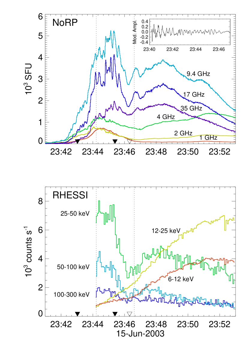
Figure 1: Top: NoRP light curves. The normalized modulation at 9.4 GHz is shown in the inset. The inverted triangles indicate the times shown in Figure 2, the open triangle indicating the time of the EIT 195Å image. Bottom: RHESSI light curves for the same time range. The vertical dashed lines indicate the time range selected for analysis.

The NoRP (Torii et al., 1979; Nakajima et al., 1985) provides total power data in total and circularly polarized intensity (Stokes parameters I and V) at 1, 2, 3.75, 9.4, 17, 35, and 80 GHz with a time resolution as high as 0.1 s. For the purposes of the analysis presented here, the data were averaged to a time resolution of 1 s. The NoRP data broaden the spectral range covered by the radio observations and provide a useful check against discrete OVSA frequency channels as well as constraints on the polarization of the observed emission. In the present case the quality of the 80 GHz data were insufficient for quantitative analysis. An overview of the NoRP observations is shown in the top panel of Figure 1.

The flare was also observed by the NoRH (Nakajima et al., 1994), which images the Sun at 17 and 34 GHz with a time resolution as high as 0.1 s. Again, in the present case, the data were averaged to a time resolution of 1 s. A time series of maps was then created in each frequency band spanning the duration of the flare. The maps were created using the AIPS software package. The AIPS task IMAGR was used to produce each map and to deconvolve the point spread function of the NoRH (the ”dirty beam”). The snapshot data were uniformly weighted, which enhances the weight given to the long antennas baselines relative to the short baselines, thereby improving the angular resolution with which the radio emission can be imaged. In the present case, the angular resolution of the maps is $15.4"\times 12.8"$ and $7.8"\times 7.1"$ at 17 and 34 GHz, respectively.

Data from RHESSI (Lin et al., 2002) are available beginning at approximately 22:44 UT. In fact, RHESSI was off-pointed from the Sun to observe the Crab nebula during June 14-15 and the flare was 1.2 to 1.5 degrees off axis, well outside the normal field of view (G. Hurford 2006, private communication). HXR photon counts were nevertheless accumulated during each half rotation of the spacecraft when its collimating grids were favorably oriented toward the flare. The data were corrected for the varying off-axis grid transmission and detector illumination and converted to one corrected count rate per spacecraft rotation. HXR light curves were obtained in five energy bands (6-12 keV, 12-25 keV, 25-50 keV, 50-100 keV, and 100-300 keV) starting at 23:42:11 UT with a time resolution of approximately 4 s. We have not imaged the data, nor do we rely on the HXR data for spectroscopic analysis. We only make use of quantities that are independent of calibration, as described further in the next section. An overview of the RHESSI data is shown in the bottom panel of Figure 1.

To summarize, our data set includes 1-18 GHz total flux density (Stokes I) spectra from OVSA, measurements of total flux and circularly polarized flux (Stokes V) from NoRP, imaging measurements at 17 (I/V) and 34 (I) GHz from NoRH, and HXR light curves in five photon energy ranges from RHESSI. We now examine the properties of the pulsations in the radio and HXR wavelength regimes.

2.2 Data Analysis and Results

2.2.1 Radio Mapping

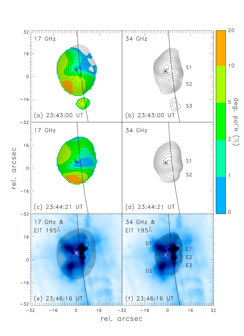
Figure 2: Overview of the radio source imaged by the NoRH at the times indicated by inverted triangles in Figure 1. The solid arc indicates the solar limb. Radio contours are at intervals of $2^{(n+1)/2}$ percent of the peak brightness temperature of each map, where $n=1,2,...12$. Color contours show the degree of polarization at 17 GHz. Panels (a) and (b) show contour maps of the 17 and 34 GHz source during the rise phase, when the peak brightness temperatures are $3.4\times 10^{7}$ K and $3.2\times 10^{6}$ K, respectively; panels (c) and (d) show the same at the time of flux maximum, when the peak brightness temperatures are $3.0\times 10^{8}$ K and $5.5\times 10^{7}$ K, respectively; panels (e) and (f) show the same superposed on the EIT 195Å. The brightness temperature maxima are $1.0\times 10^{8}$ K and $3.0\times 10^{7}$ K, respectively. The asterisk in each case shows the mean position of the quasi-periodic pulsations.

The NoRH imaging observations at 17 and 34 GHz are summarized in Figure 2 where contour maps in each frequency are shown during the rise phase (Figure 2a,b), the flux maximum (Figure 2c,d), and near the end of the first major peak of the flare when a single image from SOHO EIT at 195Å is available (Figure 2e,f). The corresponding times are indicated by inverted triangles in Figure 1. The peak brightness temperatures at each time and in each band are given in the figure caption. While a time series of such maps is available in each frequency band with a time resolution of 1 s, it is neither necessary nor practical to reproduce them all here.

The FWHM angular size of the 17 GHz source varies between $\approx\!22"\times 25"$ and $\approx\!25"\times 33"$ during the course of the flare, while the 34 GHz source varies between $\approx\!17"\times 19"$ and $\approx\!19"\times 22"$. The source is not well-resolved at 17 GHz since the angular resolution is $15.4"\times 12.8"$. The angular resolution at 34 GHz is $7.8"\times 7.1"$, however, and the source is better resolved. Figure 2b shows the 34 GHz source at 23:43:00 UT; it is composed of three components labeled S1, S2, and S3. Source S3 remains very faint during the course of the event and is not visible in subsequent images. Source S1 may correspond to a coronal loop structure, whereas source S2 is compact and unresolved. S1 is the dominant source in all contour maps shown in Figure 2 and, indeed, is the dominant source in all maps over the time range indicated by the vertical dashed lines in Figure 1. As we show in §2.2.3, it is also the source of the QPPs.

The EIT 195Å image obtained at 23:46:16 UT is complex, showing three compact bright patches inside the solar limb (labeled E1, E2, and E3); E1 and E2 are slightly saturated. Above the limb, two diffuse patches of emission are seen. It is possible that sources E1, E2, D1, and S1 are associated with a single loop or loop system, with E1 and E2 marking the footpoints. Sources E3, D2, and S2 may be associated with a separate loop or loop system that extends to the southeast. We note that soft X-ray images from the GOES 12 Soft-X-ray Imager (SXI) are also available. We find that at the time of radio maximum the SXR emission appears to originate from a single diffuse source, similar in appearance and location to the 17 GHz source. For this reason, we do not reproduce the SXI data here. The SXI data are consistent with our identification of S1 being the dominant source during the first major peak of the flare.

Maps of Stokes V are available from the NoRH at 17 GHz, and shown by the color contour map in Figure 2a and c. We find that the angular resolution at 17 GHz is insufficient to enable us to use the Stokes V maps as a basis to draw any firm conclusions regarding source morphology. We also note that since the source is near the limb, the aspect angle is far from optimum for this purpose. While we are unable to draw definite conclusions regarding the detailed source morphology in the 17 and 34 GHz bands, we can conclude that the flux density of the radio source is dominated by S1 in each band. Based on its morphology at 34 GHz (Figure 2b) we suggest that S1 may be a coronal loop.

We now turn to a more quantitative analysis of the radio and HXR QPPs. We return to the question of the source morphology in §2.2.3.

2.2.2 Modulation Amplitudes

In order to characterize the QPPs in the radio bands, we calculate the modulation power $P(f)$ and the modulation amplitude $m(f)=\sqrt{P(f)}$ for each frequency:

$$P(f)=\left<S^{2}(f,t)\right>=\frac{1}{T}\int\limits_{0}^{T}S^{2}(f,t)dt,$$ (1)

where

$$S(f,t)=\frac{F(f,t)-\left<F(f,t)\right>}{\left<F(f,t)\right>}$$ (2)

is the normalized modulation of the signal, $f$ is the frequency in GHz, $t$ is the time in seconds, $F(f,t)$ is the total flux density at frequency $f$. Similarly, a modulation amplitude can be defined for the RHESSI HXR bands, with $F(f,t)$ replaced by $C(E,t)$, where $C$ represents the photon counts s^-1 in a given energy band $E$. The brackets denote a running average of the original signal over time. The modulation amplitude is a measure of the variation of the emission with respect to the running average. While the averaging time used here for the running average is 20 s, the analysis is insensitive to the precise value used. The inset to Figure 1 shows the normalized modulation at 9.4 GHz from the beginning of the impulsive phase at 23:40 UT through the first major peak. We note the clear decline in modulation amplitude from the onset of the emission, when the modulation is $\ \raise 3.0pt\hbox{$>$}\kern-8.5pt\raise-2.0pt\hbox{$\sim$}\ 30\%$ of the mean flux, to the time of the flare maximum and later when the modulation amplitude is $\approx 10\%$ of the mean. Figure 3 displays the spectral dependence of the radio and HXR modulation amplitudes calculated for the time period 23:44:11-23:46:35 UT.

2.2.3 Fourier Analysis

The use of Fourier analysis to study radio pulsations is described by Fleishman et al. (2002a, b), who used it to study millisecond pulsations of coherent radio emission, and by Melnikov et al. (2005), who used it to study QPPs from a flare observed by the NoRH. We apply and extend that approach here, considering both multi-frequency radio and HXR data. We confine our attention to the time range 23:44:11-23:46:35 UT demarcated in Figure 1 by vertical dotted lines. The start time is determined by the availability of RHESSI data. The end time corresponds to the end of the first major peak of the cm-$\lambda$ and HXR emission (Figure 1). The results obtained for the radio emission were nevertheless checked and found to be stable against shifts in the starting and/or ending time of the interval analyzed.

The power spectrum and phase were computed from the Fourier transform of the normalized modulation for each frequency in the OVSA and NoRP data. The normalized modulation and the corresponding power spectrum are displayed for each frequency observed by the NoRP and for the nearest corresponding OVSA frequency in Figure 4. We note the presence of several peaks in each spectrum. The two most significant peaks at the optically thin frequencies of 17 and 35 GHz correspond to power at periods of $\approx\!14.5$ s and $\approx\!18.4$  s. The most significant peak at lower (optically thick) frequencies corresponds to a period near 21 s.

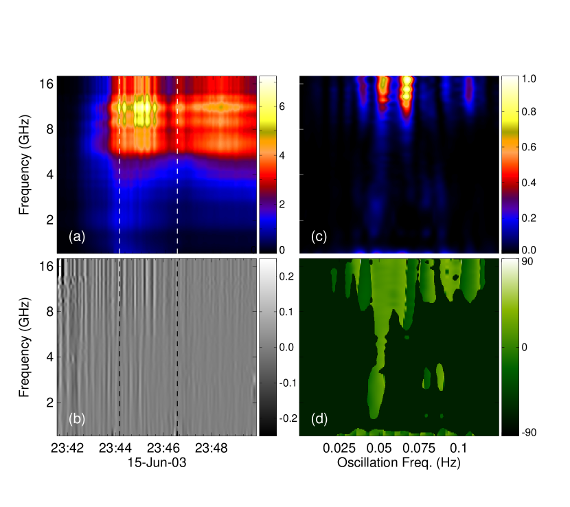
Figure 5: a) OVSA dynamic spectrum of the 1-18 GHz total intensity. The units of the intensity wedge to the right of the panel are 1000 SFU; b) the normalized modulation of the 1-18 GHz radio emission as a function of time and frequency. The scale ranges from $-25\%$ to +25%; c) the Fourier amplitude of the normalized modulation as a function of oscillation frequency and radio frequency for the time interval shown between the vertical dashed lines in panels a and b. The maximum amplitude has been scaled to 1.0; d) the Fourier phase of the normalized modulation as a function of oscillation frequency and radio frequency, again for the time range shown by the vertical dashed lines in panels a and b. The phases are scaled from $-90^{\circ}$ to $+90^{\circ}$.

Figure 5 shows a more comprehensive display of the radio oscillations in total power and their Fourier amplitudes and phases. Panel (a) shows the dynamic spectrum of the total flux density between 1-18 GHz observed by OVSA, while panel (b) shows the normalized modulation as a function of time and frequency. Panel (c) shows the Fourier amplitude of the normalized modulation as a function of the observing frequency and oscillation frequency for the time range selected for analysis. The two main amplitude peaks and subsidiary peaks are clearly seen. The corresponding phase of these peaks is shown in panel (d), indicating phase coherence over the frequency range considered. In agreement with the NoRP data, the OVSA data show a systematic change in the oscillation frequency of the dominant peak from approximately 18.4 to 21 s between 18 and 1 GHz. The phase and the corresponding time delays are shown as a function of frequency in Figure 6 for both the NoRP and OVSA data. We find that the relative phase and delay is such that lower frequencies lead higher frequencies. We note that a standard cross-correlation analysis reveals the same trends as Fourier analysis does.

We now return to the radio imaging observations obtained by the NoRH at 17 and 34 GHz to localize the primary source of the radio pulsations. We have Fourier analyzed the time series of maps in both frequency bands on a pixel by pixel basis. In this case, we are interested in which pixels dominate the net QPP amplitude (or power) and we therefore Fourier analyze $F(x,y,f,t)-\langle F(x,y,f,t)\rangle$, where the brackets again denote the running time average, for all pixels $(x,y)$ at $f=17$ and 34 GHz for the time range 23:44:11–23:46:35 UT. The result is maps of the Fourier amplitude (or power) and phase for each frequency $\tau_{P}^{-1}$ contributing to the QPPs at each spatial location. We find that the 17 and 34 GHz power spectra at the location of S1 in Figure 2 look remarkably similar to those shown for the NoRP total power measurements made at 17 and 35 GHz, shown in Figure 4.

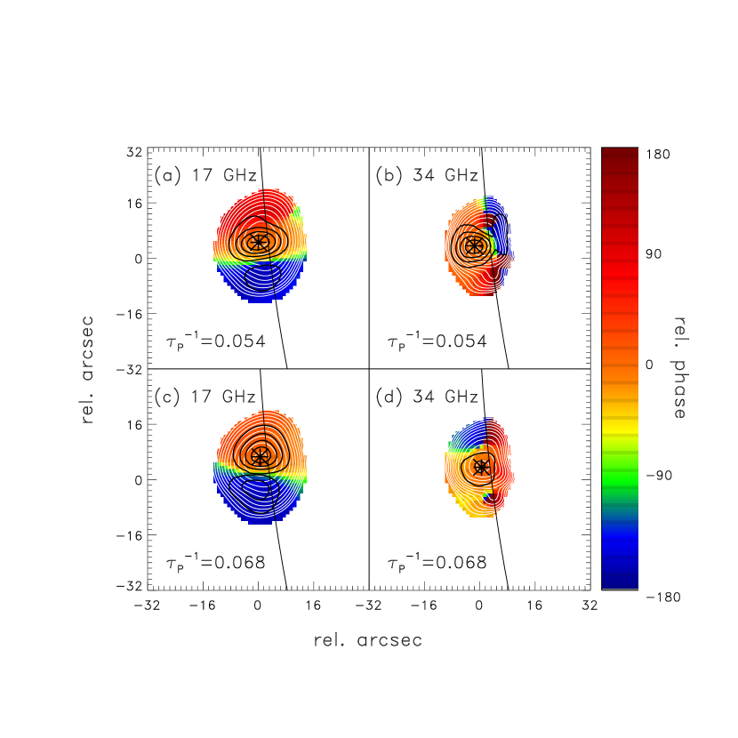
Figure 7: Each panel shows the Fourier phase (color), amplitude (black contours), and flux density at the maximum of the flare (white contours) at the radio frequency and Fourier frequency indicated. The phase in each case is referred to that at the location of the amplitude maximum, and ranges between $\pm 180^{\circ}$ (note that the dark blue and the dark red regions, showing the phase difference about 360^∘, correspond to physically the same phase). The amplitude contours are shown at 0.2, 0.4, 0.6, and 0.8 times the maximum in each panel. The white contours are the same as those shown in Figure 2c (for panels a and c) and the same as those shown in Figure 2d (for panels b and d).

Consider the two dominant peaks in the power spectra shown in Figure 4 at 9.4, 17, and 35 GHz, at frequencies corresponding to periods of 14.5 and 18.8 s. We show maps of the Fourier amplitude and phase at these two frequencies in Figure 7. The black contours represent the Fourier amplitude and the asterisk indicates the location of the amplitude maximum. The color represents the phase relative to that at the location of the asterisk in each case with dark blue representing $-180^{o}$ and dark red representing $+180^{o}$ phase shifts. The white contours show the flux density at the time of flux maximum and are identical to those show in Figure 2c,d. Figure 7 shows that the peaks at periods of 14.5 and 18.4 s are essentially co-located at both 17 and 34 GHz, that their amplitude maxima coincide with the location of S1 in Figure 2, and that they are spatially phase coherent; that is, the phase of each peak does not vary appreciably in the vicinity of the amplitude maximum in each case. We conclude that not only is the total flux at 17 and 34/35 GHz dominated by S1, the QPPs originate in S1.

Turning now to the HXR data, we also Fourier analyzed each of the five RHESSI energy ranges. Figure 8 shows the HXR normalized modulations and the corresponding power spectra for each energy range. The 17 GHz normalized modulation and power spectrum is over-plotted on four energy bands showing strongest modulations in order to compare the radio and HXR spectra. It is clear that the two most prominent peaks in the radio spectra are present in the HXR spectra, too, as well as some subsidiary peaks. The frequencies of the two main HXR peaks correspond to periods of 15 s and 19 s, similar but marginally somewhat longer than the two dominant periods in the optically thin radio emission. We again compute the (relative) phase and delay for each energy range (Figure 9). We find that the higher energy ranges tend to be progressively delayed relative to the lower energy channels.

In the remaining observational subsections we direct our attention to total power measurements of the radio emission, as observed by OVSA and NoRP, and the HXR count rates as observed by RHESSI. The optically thin radio flux density is clearly dominated by S1, as are the QPPs. Given that the dominant peak in the QPP spectra near 20 s persists at all radio frequencies between roughly 1-35 GHz in a phase coherent fashion, we conclude that the QPP source is likely localized to S1 at all frequencies. While the location of the HXR source or sources is unknown, given the similarity between the radio and HXR QPPs, they are likely intimately related, both temporally, and spatially.

2.2.4 Partial modulation amplitudes

Besides the above, the Fourier analysis allows consideration of the total modulation power (1) and the partial modulation of the signal by each pulsating component described by a Fourier peak with a finite bandwidth. The need to consider the partial modulation amplitude arises because more than one significant Fourier peak is present in the power spectrum. It is not immediately clear whether the same, or different, physical processes are responsible for each peak, e.g., some might be the result of quasiperiodic injection of fast electrons, others of MHD oscillations.

To introduce the partial modulation amplitudes we apply a fundamental property of the Fourier transform, i.e., Parceval’s identity:

$$\sum_{i=0}^{N_{i}-1}S^{2}(f,t(i))\equiv N_{tot}\sum_{n=0}^{N_{tot}-1}\mid S(f,\nu(n))\mid^{2},$$ (3)

where $N_{i}$ is the total number of the measurements in the time domain and $N_{tot}$ is the total number of the oscillation frequencies $\nu(n)$ where the Fourier amplitudes are determined. Accordingly, combining this equivalence with the definition of the total modulation power (1), we can express the modulation amplitude as a sum over all Fourier harmonics:

$$m(f)=\left(\frac{N_{tot}}{N_{i}}\sum_{n=0}^{N_{tot}-1}\mid S(f,\nu(n))\mid^{2}\right)^{1/2}.$$ (4)

The total modulation amplitude, $m(f)$, related to contribution of all available Fourier harmonics is given in Figure 3. Here we consider the partial modulation amplitudes, $m_{p}(f)$, related to modulation of the radio emission by a limited region of Fourier harmonics from $n_{1}$ to $n_{2}$ covering each of the main Fourier peaks, defined as follows:

$$m_{p}(f)=\left(2\frac{N_{tot}}{N_{i}}\sum_{n=n_{1}}^{n_{2}}\mid S(f,\nu(n))\mid^{2}\right)^{1/2},$$ (5)

where the factor 2 is related to the fact that each partial oscillation consists of two Fourier peaks with identical intensities and opposite phases.

Figure 10 displays the frequency dependence of the partial modulation amplitudes, corresponding to the two main Fourier peaks. Remarkably, the partial modulation amplitudes for all significant Fourier peaks determined with OVSA and NoRP data display similar spectral behavior, i.e., they look qualitatively similar to each other and to the total modulation amplitude presented in Figure 3. We conclude that all of the Fourier peaks are due to the same physical process.

2.2.5 Spectral Index Variations

Direct measurement of the brightness temperature of $3\times 10^{8}$ K at 17 GHz by NoRH at the time of flux maximum suggests that the corresponding brightness temperature at the spectral peak (around 10 GHz) exceeded $2\times 10^{9}$ K. This high value indicates that the spectral peak in our radio burst is formed due to the gyrosynchrotron self-absorption, rather than by Razin suppression. The observed radio emission spectrum from a flare is often characterized by a power law $F(f)\propto f^{-\beta}$, where $\beta$ is the spectral index (e.g., Bastian et al., 1998). For those frequencies where the emission is optically thin, $\beta>0$, we adopt $\beta_{\rm thin}=\beta$, and for those frequencies where the emission is optically thick, $\beta<0$, we adopt $\beta_{\rm thick}=-\beta$, so that both indices are positive. The radio spectra from OVSA and NoRP indicate that the spectral maximum of the source is $\lesssim\!10$ GHz. We have therefore formed $\beta_{\rm thin}$ using the NoRP 17 and 35 GHz observations, which are optically thin, and $\beta_{\rm thick}$ using the NoRP 3.75 and 9.4 GHz observations, which are optically thick (in fact, the 9.4 GHz emission is probably only partly optically thick, which results in a spectral index that is somewhat smaller than the true optically thick spectral index). Figure 11a shows the two spectral indices and their modulation in time. The solid line shows $\beta_{\rm thin}$ whereas the dashed line shows $\beta_{\rm thick}$ for the time range analyzed throughout this paper. $\beta_{\rm thin}$ declines systematically with time (i.e., the optically thin radio spectrum hardens) while $\beta_{\rm thick}$ remains roughly constant, but both show fluctuations similar to those seen in the radio time profile. Figure 11b shows the normalized modulation of $\beta_{\rm thin}$ and compares it with that of the 17 GHz emission. We note that the two are highly correlated. When the 17 GHz total flux is high, the spectral index is larger and the spectrum is therefore steeper (softer) and vise versa. Such a spectral behavior seems to be opposite to the standard soft-hard-soft evolution observed in individual HXR peaks (Benz et al., 2005). Figure 11c shows the same for $\beta_{\rm thick}$ and the 9.4 GHz total flux. The correlation is again excellent.

2.2.6 Polarization Variations

Finally, we consider the polarized radio emission. The degree of circular polarization, defined as $\rho_{c}(f)=V(f)/I(f)$, is plotted for 9.4 and 17 GHz in Figure 12a. The degree of polarization is quite low: only $\approx 1.5\%$ at 9.4 GHz and $5-10\%$ at 17 GHz, the latter showing a systematic decrease with time. Nevertheless, given the excellent signal to noise ratio, the normalized modulation of $\rho_{c}$ can be formed for both frequencies. Figure 12b compares the normalized oscillating component of $\rho_{\nu}$ at 9.4 GHz with that of the 9.4 GHz total flux. Figure 12c presents the same for 17 GHz. We find that the degree of polarization is anti-correlated with the radio QPPs in both cases. In other words, when the radio intensity is high, the degree of polarization is lower and when the radio intensity is low, the degree of polarization is greater.

2.3 Summary of Results

It is useful to summarize the key results from our analysis:

1. The radio and HXR flare emission display QPPs that are highly correlated with each other.

2. The radio and HXR QPPs are characterized by several significant peaks in their power spectra. The two dominant peaks correspond to periods near 15 and 20 s.

3. Both the radio flux density and the QPPs are dominated by source S1, shown in Figures 2 and 7.

4. Each of the Fourier peaks is due to the same physical process, as indicated by our partial modulation analysis.

5. The relative phase of each dominant peak shows a small, systematic shift as a function of radio frequency. The sense of the phase shift is such that the low radio frequencies lead the higher radio frequencies. A similar behavior is observed in the phase of the two dominant HXR peaks although here, it is the lower energy bands that lead the higher energy bands.

6. The total modulation power displays a systematic trend with frequency in the radio domain, the maximum modulation occurring at around 15 GHz. That is, the maximum power of the QPPs occurs somewhat above the spectral turnover.

7. Variation in the spectral index of the optically thin radio emission is correlated with variations in the radio emission. The sense of the correlation is such that the radio spectrum is steeper during QPP peaks. This is opposite from the usual soft-hard-soft behavior for X-ray peaks.

8. Variation in the degree of circular polarization, $\rho_{c}$, is anticorrelated with that in the radio flux at 9.4 and 17 GHz; i.e., $\rho_{c}$ is lowest during QPP peaks.

In light of the above findings, we now consider whether the observed QPPs are the result of MHD loop oscillations in the source, or whether they are more consistent with the quasi-periodic injection of energetic electrons into the source. Unlike many other studies, the whole body of the data available for the event under analysis allows making a firm conclusion about this.

3 Data interpretation

Electrons are accelerated and injected into coronal magnetic loops during flares. Due to the fact that coronal magnetic loops have a weaker magnetic field at the loop top than at their foot points, they act as magnetic traps. Whether an electron is trapped or not is determined by its pitch angle. The critical angle that determines precipitating vs. trapped electrons is given by $\alpha_{\rm lc}=\arcsin(B_{\rm inj}/B_{\rm loss})$, where $B_{\rm inj}$ is the magnetic field strength where the electrons are injected and $B_{\rm loss}$ is the magnetic field strength at the chromospheric height in the foot point where the electrons are collisionally removed from the trap. Electrons with sufficiently large pitch angles $\alpha>\alpha_{\rm lc}$ are trapped in the magnetic loop until they are scattered, by Coulomb collisions or wave-particle interactions, to sufficiently small pitch angles $\alpha<\alpha_{\rm lc}$, or are thermalized due to in situ Coulomb collisions. Electrons with pitch angles $\alpha<\alpha_{\rm lc}$ immediately propagate to the chromosphere, where they collide with cold ions and produce HXRs via nonthermal bremsstrahlung. Both trapped and precipitating electrons emit radio waves via nonthermal gyrosynchrotron emission. This basic picture is referred to as the ”trap plus precipitation” (TPP; Melrose & Brown, 1976) or the ”direct precipitation and trap plus precipitation” (DPTPP; Aschwanden, 1998; Aschwanden et al., 1998, 1999) model.

3.1 QPPs as the Result of MHD Oscillations

As discussed in §1, radio and HXR QPPs have been interpreted in terms of variations in the magnetic field and/or variations in the electron distribution function due to acceleration and injection. Magnetic field variations are generally attributed to MHD oscillations. A number of recent studies of cm-$\lambda$ and HXR QPPs have concluded that MHD oscillations may be the cause (Asai et al. 2001; Grechnev et al. 2003; Nakariakov et al. 2003; Melnikov et al. 2005). Among the possible oscillation modes considered were the (standing) sausage, kink, and torsional modes. Grechnev et al., studying the same event as Asai et al. (1998 November 10), also consider the possibility of magnetic field variations caused by the launch of impulsively generated, propagating MHD waves (Roberts et al., 1984) and conclude that the QPPs studied may result from either propagating MHD waves or torsional oscillations, although quasi-periodic modulation of the electron acceleration could not be definitively excluded due to lack of spectral information. Nakariakov et al. and Melnikov et al. both suggest that the QPP event of 2000 January 12 can be accounted for in terms of global sausage mode oscillations.

Can the QPPs observed from the 2003 June 15 flare be understood in terms of MHD oscillations? Certainly, the dominant periods in the oscillations are not inconsistent with possible MHD modes. As noted in §2.2, several peaks are present in the power spectra. The two strongest peaks in the radio and HXR emission have periods near 15 and 20 s. Previous authors have shown that these periods are consistent with sausage mode oscillations, fast-mode waves, and torsional oscillations (e.g., Grechnev et al. 2003). However, we can exclude each of these possibilities in the present case through consideration of the radio spectroscopic data and its polarization properties.

First, a sausage mode oscillation or the launch of fast-mode MHD waves results in a periodic compression and expansion of the magnetic flux tube in which the radiating electrons reside. Magnetic flux conservation requires a corresponding variation in the magnetic field strength and hence, a modulation of the gyrosynchrotron emissivity and the absorption coefficient. Although, the source volume and the number density of the fast electrons will be oscillating, their product will stay constant. An immediate consequence of a sausage mode oscillation is a $180^{\circ}$ phase difference between the optically thick and optically thin emission. To see this, we take the nonthermal distribution of electrons to be a power law, with $n_{nt}(E)dE\propto NE^{-\delta}dE$. Dulk (1985) gives approximate expressions for the gyrosynchrotron emissivity $\eta_{f}$, absorption coefficient $\kappa_{f}$, effective temperature $T_{eff}$, and the degree of circular polarization $\rho_{c}$, for a power law distribution of electrons that usefully illustrate the parametric dependences. For optically thin emission at a fixed frequency the radio emission $F(f)\sim\eta_{f}\propto N\ B\ s^{1.22-0.9\delta}(\sin\theta)^{-0.43+0.65\delta}$, where $s=f/f_{Be}$ is the harmonics of the electron gyrofrequency $f_{Be}=eB/2\pi m_{e}c$; $N$ is the total number of nonthermal electrons above some threshold energy $E_{\circ}$; and $\theta$ is the angle between the magnetic field vector and the line of sight. For a fixed frequency $f$, the relation implies $F(f)\propto B^{0.9\delta-0.22}$. Hence, for any plausible value of $\delta$, the optically thin emission increases with increasing magnetic field strength. In contrast, for optically thick emission at a fixed frequency, $F(f)\sim\eta_{f}/\kappa_{f}\propto T_{eff}\propto s^{0.5+0.085\delta}(\sin\theta)^{-0.36-0.06\delta}$. Again, for fixed conditions, $F(f)\propto B^{-0.5-0.085\delta}$ and the optically thick emission decreases with increasing magnetic field.

For a global sausage mode oscillation, therefore, variations in the optically thick emission are expected to be anticorrelated with those seen in the optically thin emission. The same conclusion can be drawn for propagating waves in the magnetic loop. However, as shown in §2.2.1 and Figure 6, this is not the case. Instead of a large, 180-degree sharp phase shift from optically thick to optically thin frequencies, only a slow gradual variation of oscillation phase is seen. One can easily check that, similar to the global sausage mode, the low spatial harmonics of the sausage mode loop oscillations fail to provide a reasonable fit to the phase variations presented in Figure 6 even in the case of nonuniform magnetic loop.

Consider instead a torsional oscillation which results in a variation of the magnetic field vector to the line of sight. For optically thin emission, the dependence of the emissivity on the angle $\theta$ between the line of sight and the magnetic field vector is $\eta_{f}\propto(\sin\theta)^{-0.43+0.65\delta}$ while for optically thick emission we have $T_{eff}\propto(\sin\theta)^{-0.36-0.06\delta}$. Again, we expect the optically thick and optically thin emission to be anti-correlated, which is not observed.

The polarization data can in principle constrain the underlying physical model (e.g., Altyntsev et al., 2008). However, the radio source is located close to the limb so that the polarization can be strongly affected by propagation effects and, moreover, the source is not well spatially resolved, see Figure 2. Therefore, we only rely here on the relative variations and trends of the degree of polarization rather than on its absolute value. The degree of circular polarization from optically thin emission is $\rho_{c}\propto s^{-0.78+0.55\cos\theta}\propto B^{0.78-0.55\cos\theta}$ (Dulk 1985) so it is expected to increase with magnetic field and hence, with the emissivity. Therefore, variations in $\rho_{c}$ should be correlated with variations in the flux density in optically thin frequencies if MHD oscillations are relevant. The observations show, however, that $\rho_{c}$ is instead anticorrelated with flux variation at 17 GHz (Figure 12).

Understanding the time variation of the spectral index and its correlation with radio emission (Figure 11) is also problematic in the context of MHD oscillations. While variations in the magnetic field due to oscillations yield variations in the (perpendicular component) of the electron energy due to betatron acceleration, no change is expected in the electron spectral index $\delta$ of a power-law distribution of electrons (see, e.g., Bogachev & Somov, 2007) and therefore, no change in the radio spectral index at optically thin frequencies. However, oscillations of the magnetic field can give rise to radio spectral index variations at fixed frequencies because for stronger magnetic field the spectral peak moves towards higher frequencies, making the spectrum at fixed frequencies above the peak slightly flatter. In our event, however, the radio spectrum is steeper when the emission is stronger.

Finally, consider whether MHD oscillations can provide a reasonable quantitative fit to the spectral behavior of the modulation amplitude. To achieve this goal we start from a uniform source model, whose radio emission is described by simplified Dulk and Marsh formulae (Dulk, 1985). Although those formulae have a somewhat limited range of applicability, they nevertheless provide useful insights into the parametric dependences and corresponding trends. Note that the use of the Dulk and Marsh approximation means that we did not consider the Razin-effect, but rather assume that the spectral peak is determined by the effect of optical thickness, which is directly confirmed by the high brightness temperature determined from imaging radio measurements, (see caption to Figure 2).

To model an MHD oscillation, we assume sinusoidal oscillations of the magnetic field at the source

$$B=B_{0}+\Delta B\sin\omega t.$$ (6)

Note, that depending on the specific mode of the magnetic oscillations, some other parameters of the source (volume, density etc.) may or may not oscillate. Although we examined a few particular cases, we present here a model with a simple loop oscillation (i.e., global sausage mode) taking into account the conservation of the magnetic flux through the source, which implies: $S\propto B_{0}/B$, where $S$ is the source area, and $N_{e}\propto B/B_{0}$. Other models that we have considered yield similar conclusions.

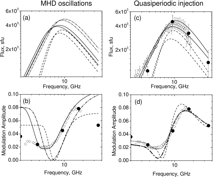
Figure 13: Model gyrosynchrotron spectra (the pairs show two extremes as the spectrum oscillates for each case) and modulation amplitudes for the cases of MHD global sausage mode oscillations (left) and quasiperiodic injection (right). Dashed curves are calculated for a uniform model, while the dash-dotted and solid curves for simplified inhomogeneous models. In the left column the non-uniform spectra differ from each other: dash-dotted curves provide good spectrum fit (a), but fail to account the modulation amplitude (b), while solid curves suggest the best fit to the modulation amplitude (b), but fail to provide a reasonable spectrum fit (a). The solid curve in the panel (d), providing an excellent fit to the data, is calculated for the inhomogeneous model with an unrelated noise contribution added with the frequency-independent rms value of 1.7$\%$. The corresponding solid and dash-dotted spectra are undistinguishable in the panel (c). The diamonds show the OVSA data, while the filled circles show the NoRP data. A composite observed spectrum (diamonds and circles) displayed in panel (c) shows the mean values of the radio flux as observed for the first 80 s of the analyzed data fragments, while the corresponding error bars display the whole range of the flux variation during these 80 s. We do not show this spectrum in panel (a) to keep it clearly readable.

Specifically, dashed curves in Figure 13 are calculated for the uniform model, which are in obvious disagreement with the data. Although we are able to match a considerable part of the modulation amplitude curve, the model and observations clearly diverge at low and high frequencies. A possible reason for this is oversimplified model relying on an uniform radio source. Indeed, we have clear observational evidence of the source inhomogeneity: the observed optically thick spectrum is much flatter ($\sim f^{1.5}$) than the theoretical one for the uniform source ($\sim f^{2.5-3}$).

Accordingly, to improve the spectral fit to the data, we introduce a simplified non-uniform model, which takes into account the source inhomogeneity assuming slower (than for the uniform case) increase of the gyrosynchrotron optical depth with frequency decrease to match the observed low-frequency slope of the spectrum. Specifically, we adopted $\tau=\tau_{0}(f/9~{}\hbox{GHz})^{1.1}$, where $\tau_{0}$ is the optical depth for the uniform source (Dulk & Marsh, 1982). To justify this simplified non-uniform model we note that in the optically thick case the emission comes from a thin layer having the optical depth of about 1 in both uniform and inhomogeneous cases. In the inhomogeneous case, however, the physical size of this layer can decrease more slowly than in the uniform case, giving rise to a flatter low-frequency spectrum, which is taken into account within our simplified model.

The corresponding model (dash-dotted curves) gives a reasonable spectral fit, but does not at all improve the fit of the modulation amplitude vs frequency. Adding some portion of unrelated noise to the model improves the fit slightly. The model providing the best fit (solid lines) to the observed modulation amplitude yields $B_{0}\approx 540$ G and $\Delta B/B_{0}\approx 0.06$ and a low level of the unrelated noise 1.7$\%$. However, if we tweak the model for the best fit to the modulation amplitude data (solid line), the model gives a poor fit to the power spectrum. In particular, the model spectral peak frequency is significantly lower than the observed one. In contrast, if we match the observed spectrum (dash-dotted line), we cannot get a reasonable fit to the modulation amplitude. Overall, irrespectively to the details adopted, the model of the MHD oscillation strongly overestimates the modulation amplitude at low and high frequencies.

We conclude that while the periods of the QPPs at HXR and radio wavelengths are consistent with MHD modes that could be supported by a coronal magnetic loop, a more detailed analysis of the observations shows that MHD oscillations fail to account for most of the observed properties of the QPPs. We conclude that MHD loop oscillations are not relevant to the flare studied here.

3.2 QPPs as a Result of Electron Acceleration and Injection

We now consider whether quasi-periodic electron acceleration and injection can satisfactorily account for the observations. In particular, we suggest that each peak in the radio and HXR emission corresponds to a discrete injection of fresh electrons into the magnetic loop. The modulation amplitude of the radio emission, which is comparable with that of HXR emission, as well as the short decay time of the radio pulses, suggest that the newly injected fast electrons have a rather short life time, a few seconds. It is unlikely that the short electron life time is due to Coulomb losses in the loop, since this would require a rather high plasma density $n>3\times 10^{11}$ cm^-3 that would, in turn, result in strong Razin suppression of the radio emission at low frequencies and also in a spectral peak well above 10 GHz, which are not observed. Therefore, the most probable reason of the rapid loss of the energetic electrons is emptying of the loss-cone by precipitation. This idea, corresponding to the DPTPP model, has several consequences.

First, the correlation between the radio and HXR emission is easily explained. With each new injection of electrons into the trap, the optically thin emission increases as $F(f)\propto N$ and the electrons filling the loss cone directly precipitate from the loop, producing enhanced HXR emission. Those electrons with large enough pitch angles accumulate in the trap, where their energy distribution is expected to collisionally harden.

In contrast to the case of MHD oscillations, the phase of the Fourier components is not expected to change between optically thick and thin emission. Moreover, the amplitude of the oscillation is expected to greatly diminish as emission transitions from optically thin to optically thick radio emission. The observations are qualitatively consistent with these expectations. This alone is sufficient to argue strongly for quasi-periodic injection of particles as the cause of the oscillations. However, the observations are sufficiently complete that we can investigate the oscillations in greater detail. Specifically, the phase of the dominant Fourier peak varies systematically from high to low frequencies, corresponding to a relative timing delay between frequencies. The sense of the delay is such that high frequencies/energies lag low frequencies/energies. Since the radio frequencies/X-ray energies are, broadly speaking, proportional to electron energy, these observations imply that the acceleration and injection of higher energy electrons in each oscillation lag the lower energy electrons. It automatically follows that the spectral index of the injected electrons must be modulated.

These ideas can be captured in a simplified phenomenological model of the periodic injection of energetic electrons into the magnetic loop. The number density of nonthermal electrons $N_{e}$ is taken to be a superposition of periodically injected electrons $\Delta N_{e}$ and those electrons that have accumulated in the magnetic trap $N_{e0}$:

$$N_{e}=N_{e0}+\Delta N_{e}|\sin\omega t|.$$ (7)

In addition, we assume that the electron spectral index at the source varies almost synchronously with the number density, although with a small phase shift, which agrees with that in Figure 11:

$$\delta=\delta_{0}+\Delta\delta|\sin(\omega t+\varphi_{\delta})|.$$ (8)

The relative variation of the spectral index, $\Delta\delta/\delta=0.08$, and the phase $\varphi_{\delta}\approx\pi/16$ are taken to provide a change in radio spectral index $\Delta\beta/\beta\approx 0.08$ and the corresponding time shift that agrees with Figure 11b, while the value $\Delta N_{e}(>100~{}keV)/N_{e}(>100~{}keV)\approx 0.6$ is selected to match the modulation amplitude in the range of the radio spectral peak. The magnetic field at the source is taken to be $B=650$ G, which provides the correct radio flux density and spectral peak frequency $f_{\rm peak}$ near $\sim\!10$ GHz.

Figure 13, right column, displays the spectra and the modulation amplitude for the quasi-periodic injection model along with the respective measurements. As in the previous section, dashed curves in Figure 13 are calculated for a uniform model, and are in qualitative agreement with the observed modulation amplitude. However, the fit to the observed spectrum can be improved using a non-uniform model, as has been explained in the previous section.

The simplified non-uniform model simultaneously gives a reasonable spectral fit (dash-dotted curves) and a better approximation to the modulation amplitude vs. frequency. The remaining discrepancy near the minimum of the curve is surprisingly low. It can be adjusted by adding 1.7$\%$ unrelated noise as was also necessary for the MHD model in Figure 13b. This level is only about 20-30 sfu at the frequencies near the minimum. Such a small residual oscillation does not affect the spectrum itself (Figure 13c). The corresponding (solid) curve provides an excellent fit to the modulation amplitude data (Figure 13d) showing that the simplified model can account for the observations assuming only quasi-periodic injection of the fast electrons into the radio source. Although we fit here the total modulation amplitude of the radio emission, we note that all partial modulation amplitudes (including those given in Figure 10) behave qualitatively similarly, therefore, all oscillations found in the radio data should be ascribed to the same process.

To account for the observed anti-correlation between flux density variations and polarization (Figure 12a), we find a natural explanation in a systematic variation in pitch-angle anisotropy of the electrons. Fleishman & Melnikov (2003) have shown that the degree of polarization of optically thin gyrosynchrotron emission at a fixed frequency increases as the degree of perpendicular anisotropy in the electron distribution function increases. Assuming for simplicity that the electrons are injected with an isotropic distribution, after some time the loss cone will empty due to escape of electrons from the trap, and the pitch angle distribution of the remaining, trapped electrons becomes anisotropic, leading to an increase in polarization.

To summarize, we find that the observed properties of the QPPs in the 15 June 2003 flare are consistent with the quasi-periodic injection of energetic electrons into a coronal magnetic loop. The injected electrons show an evolution wherein more energetic electrons are delayed relative to less energetic electrons. This manifests itself in a quasi-periodic modulation of the index $\delta$. With each fresh injection of electrons, those with small pitch angles directly precipitate from the trap, producing HXR emission. The distribution of those electrons that remain trapped collisionally hardens (Melnikov, 1994), yielding systematic trends in the radio spectral index $\beta_{\rm thin}$ and $\rho_{c}$, both of which decrease in time for optically thin emission. All of the essential features of the radio and HXR QPPs are consistent with the DPTPP picture.

4 Discussion

In this paper we present a detailed quantitative analysis of the radio and HXR QPPs in a solar flare and fit the data assuming two competing models – one model involving MHD loop oscillations and the other model involving quasiperiodic injection/acceleration of nonthermal electrons. We find, using the complete spectral information available for this event, that it is not possible to get a consistent fit to the data within the magnetic oscillation model. By comparison, the model with quasiperiodic particle injection offers an excellent fit to the variations in radio flux density, power-law index, and polarization, as well as their correlations with each other and with hard X-ray QPPs.

Although in principle one might expect a loop with quasi-periodic injection to respond with MHD oscillations of some type, our analysis of partial modulation amplitude suggests that all of the significant periods (peaks of the Fourier spectrum) are due to quasi-periodic injection of the fast electrons into the source. This fact implies that the magnetic loop comprising the radio source either is a rather bad resonator or has no eigen-mode in the considered range of the oscillation periods (in essence, above 0.2 s). Indeed, if the loop could support the corresponding oscillations, it would respond on the quasi-periodic particle injection by displaying an appropriate eigen-mode of the loop oscillation, which is not observed.

The modulation amplitude of the gyrosynchrotron (GS) emission, which is comparable with that of HXR emission, as well as the short decay time of the radio pulses, suggest that the newly injected fast electrons have a rather small life time (  $<$$\sim$   few s). That short life time can hardly be provided by the Coulomb losses in the loop, since this would require a high plasma density $n>3\times 10^{11}$cm^-3 resulting in strong Razin suppression, which we have argued is inconsistent with the observations. Therefore, the most probable reason for the rapid loss of the energetic electrons is emptying of the loss-cone by precipitation, which also accounts for the excellent degree of correlation between the radio and HXR QPPs and the polarization properties of the event.

Finally, we note that this event is similar in many respects to the celebrated flare of 7 June 1980, discussed in great detail by Kane et al. (1983). In particular, Kane et al. also reported an anti-correlation between the degree of polarization and the flux density at 17 GHz. Because the spectral peak of the emission in that event was $\gtrsim 17$ GHz, so that optical depth effects may be important, we choose 9.4 GHz in our event for a direct comparison. The 9.4 GHz emission for the 15 Jun 2003 event, like the 17 GHz emission for the 7 Jun 1980 flare, is marginally optically thick. The normalized modulations of the intensity and polarization at 9.4 GHz in our event are indeed anti-correlated (see Figure 12), and similar in value to those at 17 GHz in the 1983 event. Although Kane et al. do not suggest an interpretation of the polarization oscillations, they conclude that quasiperiodic electron acceleration and injection are responsible for the 1983 event. We find that the variation of the angular particle distribution during the quasiperiodic electron injection results naturally in the oscillations of the degree of polarization, as observed in both Kane’s and our events, which eventually confirms the Kane et al. choice in favor of the quasiperiodic injection/acceleration in that event.

5 Conclusions

We described an oscillating event observed with high spectral resolution in the microwave range and analyzed it by applying and developing further the Fourier method presented earlier by Fleishman et al. (2002b, a); Melnikov et al. (2005). We developed the idea of partial modulation amplitudes, expressed as the modulation amplitude in each particular Fourier peak of finite bandwidth, using the Parseval identity. In the general case the method is capable of distinguishing different simultaneous contributions to the overall modulation of the radio emission, which might be especially powerful when both MHD oscillations and quasiperiodic electron injection contribute to QPPs of the radio emission. For our event this method showed that all of the Fourier harmonics have the same characteristics, i.e. are all due to quasiperiodic injection of the electrons in the radio source. Thus, we conclude that for this event MHD oscillations play no role. Possibly, this result calls into question some previous studies, which concluded that MHD oscillations play a key role in the radio and HXR QPPs, but which did not have the complete spectral information needed to apply our method of analysis.

Specifically, QPPs in our event had the following characteristics:

$\bullet$ The Fourier spectrum at each observing frequency is composed of a few significant peaks, corresponding to a few oscillation quasi-periods.

$\bullet$ None of the main radio Fourier peaks could be interpreted as the result of MHD loop oscillations.

$\bullet$ Several measures, e.g., modulation amplitudes of the flux density as a function of radio frequency or photon energy, the relative phases of the oscillations as a function of frequency, the spectral indices of the radio emission, and the degree of polarization are inconsistent with MHD loop oscillations, but are fully consistent with quasi-periodic acceleration and injection of electrons as the cause of the observed radio and X-ray QPPs.

$\bullet$ Rather strong QP energy release and particle injection appears not to have excited MHD oscillations, hence, the corresponding loop is a rather bad resonator in the range of oscillation frequencies under discussion.

The spatial resolution of the available data is insufficient to address the physical cause of the observed quasiperiodic injection of fast electrons. Several mechanisms have been advanced in the literature, such as a nonlinear self-organizing regime of the electron acceleration (e.g., Aschwanden, 1987) or bursty reconnection during a plasmoid ejection (Kliem et al., 2000) or during the interaction of current carrying loops (Sakai & Ohsawa, 1987). In any case, acceleration of fast electrons in the form of distinct, quasi-periodic injections seems to be rather common in solar flares, see, e.g., (Aschwanden et al., 1998; Benz et al., 2005; Altyntsev et al., 2008). In many events, the accumulation of the electrons in the magnetic loop due to the trapping effect results in smooth light curves, making it difficult to distinguish the contributions from these distinct injections. In some favorable conditions, however, when these injections are comparable in strength, more or less equidistant in time, and the fraction of directly precipitating electrons is relatively large, such repetitive electron injections manifest themselves as pronounced broadband pulsations of the radio emission, as in the instance considered in this paper.

We conclude that radio and X-ray spectral data, when available, should be used along with imaging observations to firmly determine whether QPPs are produced by quasiperiodic injection of fast electrons into a magnetic loop or some MHD oscillating mode of the loop. The method of partial modulation amplitudes should even be able to distinguish cases when both processes are operating simultaneously.

Figure 3: The modulation amplitude of the radio emission (left) obtained with OVSA (diamonds in both this and further figures) and NoRP (filled circles in both this and further figures) calculated with Eq.(1) for the selected time interval and of X-ray emission (asterisks, right in both this and further figures).

Figure 4: The normalized modulation of the NoRP and OVSA data (left) and the corresponding power spectra (right). The two most prominent peaks in the top three panels of the power spectra correspond to periods $\tau_{P}$ of approximately 19 s and 15 s. A lower-amplitude peak appears at a period of approximately 10 s. The lower three panels (note the change of scale) display a common peak near a period $\tau_{P}\approx 21$ s.

Figure 6: Phase differences and corresponding time delays for two main Fourier peaks. The mean value of the frequency-dependent period (see Figure 5) indicated on top of each panel is taken to calculate the time delay.

Figure 8: The normalized modulations of the RHESSI data (left) and the corresponding power spectra (right). The normalized modulation of the NoRP 17 GHz emission is plotted as a thin solid line over the 12-25, 25-50, 50-100, and 100-300 keV normalized modulations in the left panel. The 17 GHz power spectrum is plotted as a dashed line on the corresponding HXR power spectra.

Figure 9: Phase differences and corresponding time delays for two main Fourier peaks available in Figure 8.

Figure 10: Partial modulation amplitudes related to limited range of Fourier harmonics around two main Fourier peaks ($\tau_{P}\approx$19 s, left, and $\tau_{P}\approx$15 s, right).

Figure 11: a) The solid line shows the spectral index of optically thin emission $\beta_{\rm thin}$, calculated between 17 and 35 GHz. The dashed line shows the spectral index of optically thick emission $\beta_{\rm thick}$, calculated between 3.75 and 9.4 GHz. b) The normalized modulation of the optically thin spectral index $\beta_{\rm thin}$ compared with that of the 17 GHz emission. c) The normalized modulation of the optically thick spectral index $\beta_{\rm thick}$ compared with that of the 9.4 GHz emission.

Figure 12: a) Degree of polarization of the 17 GHz (solid) and 9.4 GHz (dotted) emission; b) The normalized modulation of the 9.4 GHz degree of polarization (solid) compared with that of the 9.4 GHz total flux (dotted); c) The normalized modulation of the 17 GHz degree of polarization (solid) compared with that of the 17 GHz total flux (dotted).

References

- Abrami (1970) Abrami, A. 1970, Sol. Phys., 11, 104
- Abrami (1972) —. 1972, Nature, 238, 25
- Altyntsev et al. (2008) Altyntsev, A. T., Fleishman, G. D., Huang, G.-L., & Melnikov, V. F. 2008, ApJ, 677, 1367
- Asai et al. (2001) Asai, A., Shimojo, M., Isobe, H., Morimoto, T., Yokoyama, T., Shibasaki, K., & Nakajima, H. 2001, ApJ, 562, L103
- Aschwanden (1987) Aschwanden, M. J. 1987, Sol. Phys., 111, 113
- Aschwanden (1998) —. 1998, ApJ, 502, 455
- Aschwanden & Benz (1986) Aschwanden, M. J. & Benz, A. O. 1986, A&A, 158, 102
- Aschwanden & Benz (1988) —. 1988, ApJ, 332, 466
- Aschwanden et al. (1999) Aschwanden, M. J., Fletcher, L., Sakao, T., Kosugi, T., & Hudson, H. 1999, ApJ, 517, 977
- Aschwanden et al. (1995) Aschwanden, M. J., Montello, M. L., Dennis, B. R., & Benz, A. O. 1995, ApJ, 440, 394
- Aschwanden et al. (1998) Aschwanden, M. J., Schwartz, R. A., & Dennis, B. R. 1998, ApJ, 502, 468
- Aschwanden et al. (1985) Aschwanden, M. J., Wiehl, H. J., Benz, A. O., & Kane, S. R. 1985, Sol. Phys., 97, 159
- Bardakov & Stepanov (1979) Bardakov, V. M. & Stepanov, A. V. 1979, Soviet Astronomy Letters, 5, 247
- Bastian et al. (1998) Bastian, T. S., Benz, A. O., & Gary, D. E. 1998, ARA&A, 36, 131
- Benz et al. (2005) Benz, A. O., Grigis, P. C., Csillaghy, A., & Saint-Hilaire, P. 2005, Sol. Phys., 226, 121
- Bernold (1980) Bernold, T. 1980, A&AS, 42, 43
- Bogachev & Somov (2007) Bogachev, S. A. & Somov, B. V. 2007, Astronomy Letters, 33, 54
- Chen & Yan (2007) Chen, B. & Yan, Y. 2007, Sol. Phys., 246, 431
- Chiu (1970) Chiu, Y. T. 1970, Sol. Phys., 13, 420
- Dröge (1967) Dröge, F. 1967, Z. Astrophys., 66, 214
- Dröge (1977) —. 1977, A&A, 57, 285
- Dulk (1985) Dulk, G. A. 1985, ARA&A, 23, 169
- Dulk & Marsh (1982) Dulk, G. A. & Marsh, K. A. 1982, ApJ, 259, 350
- Elgarøy & Sveen (1973) Elgarøy, Ø. & Sveen, O. P. 1973, Sol. Phys., 32, 231
- Fleishman et al. (2002a) Fleishman, G. D., Fu, Q. J., Huang, G.-L., Melnikov, V. F., & Wang, M. 2002a, A&A, 385, 671
- Fleishman et al. (2002b) Fleishman, G. D., Fu, Q. J., Wang, M., Huang, G.-L., & Melnikov, V. F. 2002b, Phys. Rev. Lett., 88, 251101
- Fleishman & Melnikov (2003) Fleishman, G. D. & Melnikov, V. F. 2003, ApJ, 587, 823
- Fleishman et al. (1994) Fleishman, G. D., Stepanov, A. V., & Yurovsky, Y. F. 1994, Sol. Phys., 153, 403
- Gary & Hurford (1994) Gary, D. E. & Hurford, G. J. 1994, ApJ, 420, 903
- Gotwols (1972) Gotwols, B. L. 1972, Sol. Phys., 25, 232
- Grechnev et al. (2003) Grechnev, V. V., White, S. M., & Kundu, M. R. 2003, ApJ, 588, 1163
- Hurford et al. (1984) Hurford, G. J., Read, R. B., & Zirin, H. 1984, Sol. Phys., 94, 413
- Janssens et al. (1973) Janssens, T. J., White, K. P., & Broussard, III, R. M. 1973, Sol. Phys., 31, 207
- Kane et al. (1983) Kane, S. R., Kai, K., Kosugi, T., Enome, S., Landecker, P. B., & McKenzie, D. L. 1983, ApJ, 271, 376
- Karlický & Bárta (2007) Karlický, M. & Bárta, M. 2007, A&A, 464, 735
- Kliem et al. (2000) Kliem, B., Karlický, M., & Benz, A. O. 2000, A&A, 360, 715
- Korsakov & Fleishman (1998) Korsakov, V. B. & Fleishman, G. D. 1998, Radiophysics and Quantum Electronics, 41, 28
- Kurths et al. (1991) Kurths, J., Benz, A. O., & Aschwanden, M. J. 1991, A&A, 248, 270
- Li et al. (1987) Li, H.-W., Zlobec, P., & Messerotti, M. 1987, Sol. Phys., 111, 137
- Lin et al. (2002) Lin, R. P., Dennis, B. R., Hurford, G. J. et al. 2002, Sol. Phys., 210, 3
- Magdalenić et al. (2002) Magdalenić, J., Zlobec, P., Messerotti, M., & Vršnak, B. 2002, in ESA Special Publication, Vol. 506, Solar Variability: From Core to Outer Frontiers, ed. J. Kuijpers, 331–334
- McLean & Sheridan (1973) McLean, D. J. & Sheridan, K. V. 1973, Sol. Phys., 32, 485
- McLean et al. (1971) McLean, D. J., Sheridan, K. V., Steward, R. T., & Wild, J. P. 1971, Nature, 234, 140
- Meerson et al. (1978) Meerson, B. I., Sasorov, P. V., & Stepanov, A. V. 1978, Sol. Phys., 58, 165
- Melnikov (1994) Melnikov, V. F. 1994, Radiophysics and Quantum Electronics, 37, 557
- Melnikov et al. (2005) Melnikov, V. F., Reznikova, V. E., Shibasaki, K., & Nakariakov, V. M. 2005, A&A, 439, 727
- Melrose & Brown (1976) Melrose, D. B. & Brown, J. C. 1976, MNRAS, 176, 15
- Mészárosová et al. (2005) Mészárosová, H., Rybák, J., Zlobec, P., Magdalenić, J., Karlický, M., & Jiřička, K. 2005, in ESA Special Publication, Vol. 600, The Dynamic Sun: Challenges for Theory and Observations
- Nakajima et al. (1983) Nakajima, H., Kosugi, T., Kai, K., & Enome, S. 1983, Nature, 305, 292
- Nakajima et al. (1994) Nakajima, H., Nishio, M., Enome, S., Shibasaki, K., Takano, T., Hanaoka, Y., Torii, C., Sekiguchi, H., Bushimata, T., Kawashima, S., Shinohara, N., Irimajiri, Y., Koshiishi, H., Kosugi, T., Shiomi, Y., Sawa, M., & Kai, K. 1994, IEEE Proceedings, 82, 705
- Nakajima et al. (1985) Nakajima, H., Sekiguchi, H., Sawa, M., Kai, K., & Kawashima, S. 1985, PASJ, 37, 163
- Nakariakov et al. (2003) Nakariakov, V. M., Melnikov, V. F., & Reznikova, V. E. 2003, A&A, 412, L7
- Nakariakov & Stepanov (2007) Nakariakov, V. M. & Stepanov, A. V. 2007, in Lecture Notes in Physics, Berlin Springer Verlag, Vol. 725, Lecture Notes in Physics, Berlin Springer Verlag, ed. K.-L. Klein & A. L. MacKinnon, 221–250
- Nindos & Aurass (2007) Nindos, A. & Aurass, H. 2007, in Lecture Notes in Physics, Berlin Springer Verlag, Vol. 725, Lecture Notes in Physics, Berlin Springer Verlag, ed. K.-L. Klein & A. L. MacKinnon, 251–277
- Parks & Winckler (1969) Parks, G. K. & Winckler, J. R. 1969, ApJ, 155, L117
- Pick & Trottet (1978) Pick, M. & Trottet, G. 1978, Sol. Phys., 60, 353
- Roberts et al. (1984) Roberts, B., Edwin, P. M., & Benz, A. O. 1984, ApJ, 279, 857
- Rosenberg (1970) Rosenberg, H. 1970, A&A, 9, 159
- Rosenberg (1972) —. 1972, Sol. Phys., 25, 188
- Sakai & Ohsawa (1987) Sakai, J.-I. & Ohsawa, Y. 1987, Space Science Reviews, 46, 113
- Slottje (1981) Slottje, C. 1981, Atlas of Fine Structures of Dynamic Spectra of Solar Type IV-dm and Some Type II Radio Bursts (The Netherlands: Dwingeloo, 1981)
- Stepanov et al. (2004) Stepanov, A. V., Kopylova, Y. G., Tsap, Y. T., Shibasaki, K., Melnikov, V. F., & Goldvarg, T. B. 2004, Astronomy Letters, 30, 480
- Stepanov & Yurovsky (1990) Stepanov, A. V. & Yurovsky, Y. F. 1990, Soviet Astronomy Letters, 16, 106
- Torii et al. (1979) Torii, C., Tsukiji, Y., Kobayashi, S., Yoshimi, N., Tanaka, H., & Enome, S. 1979, Proc. of the Res. Ist. of Atmospherics, Nagoya Univ., 26, 129
- Trottet et al. (1981) Trottet, G., Kerdraon, A., Benz, A. O., & Treumann, R. 1981, A&A, 93, 129
- Young et al. (1961) Young, C. W., Spencer, C. L., Moreton, G. E., & Roberts, J. A. 1961, ApJ, 133, 243
- Yurovsky (1991) Yurovsky, Y. F. 1991, Soviet Astronomy Letters, 17, 268
- Zaitsev & Stepanov (1975a) Zaitsev, V. V. & Stepanov, A. V. 1975a, Issledovaniia Geomagnetizmu Aeronomii i Fizike Solntsa, 37, 3
- Zaitsev & Stepanov (1975b) —. 1975b, Issledovaniia Geomagnetizmu Aeronomii i Fizike Solntsa, 37, 11
- Zaitsev & Stepanov (1982a) —. 1982a, Soviet Astronomy Letters, 8, 132
- Zaitsev & Stepanov (1982b) —. 1982b, Soviet Astronomy, 26, 340
- Zlobec et al. (1987) Zlobec, P., Messerotti, M., Comari, M., Li, H.-W., & Barry, M. B. 1987, Sol. Phys., 114, 375