Spin-wave dispersion and exchange stiffness in Nd₂Fe₁₄B and $R$Fe₁₁Ti ($R$=Y, Nd, Sm) from first-principles calculations

Abstract

We theoretically investigate spin-wave dispersion in rare-earth magnet compounds by using first-principles calculations and a method we call the reciprocal-space algorithm (RSA). The value of the calculated exchange stiffness for Nd₂Fe₁₄B is within the range of reported experimental values. We find that the exchange stiffness is considerably anisotropic when only short-range exchange couplings are considered, whereas inclusion of long-range couplings weakens the anisotropy. In contrast, $R$Fe₁₁Ti ($R$=Y, Nd, Sm) shows large anisotropy in the exchange stiffness.

I Introduction

Finite-temperature properties of magnetic materials are one of the central interests in the development of permanent magnets not only from a fundamental point of view but also from a technological point of view, because magnets are used at and above room temperature in industrial applications. Modern high-performance permanent magnets are rare-earth magnets, and their main phases are rare-earth transition-metal compounds. The magnet compound Nd₂Fe₁₄B is the main phase of the neodymium magnet, which is often said to be the strongest magnet. $R$Fe₁₂-type compounds with a ThMn₁₂-type structureHirayama et al. (2017) have also attracted attention as potential main phases of magnets for surpassing the neodymium magnet.

Spin-wave frequency is a fundamental quantity for studying magnetic properties at finite temperatures. It is a collective and elementary excitation in magnetic materials. The curvature of its lowest branch at the $\Gamma$ point is called the spin-wave stiffness and is proportional to the exchange stiffness. Experimentally, the spin-wave stiffness can be measured directly by neutron scattering or by deduction from the magnetization curve versus temperature on basis of Bloch’s $T^{3/2}$ law.

For example, the exchange stiffness of Nd₂Fe₁₄B as determined by neutron scattering experiments was reported by Mayer et al.Mayer et al. (1991, 1992) and by Ono et al.Ono et al. (2014) In addition, inelastic neutron scattering was recently reported in a study by Naser et al.Naser et al. (2020) Although Mayer et al. observed no significant difference in the spin-wave dispersion along the $a$ direction and the $c$ direction, Naser et al. argued that the exchange stiffness has significant anisotropy below room temperature, where the stiffness in the $c$ direction ($A_{z}$) is smaller than in the $a$ direction ($A_{x}$).

From a theoretical point of view, the exchange stiffness is a basic input parameter in micromagnetic simulations. Although experimental values are used in most simulations, recent efforts have been made to determine the exchange stiffness theoretically based on first-principles calculations. Toga et al. derived a classical Heisenberg model of Nd₂Fe₁₄B from the results of density functional calculations.Toga et al. (2018) The model thus obtained was analyzed by Monte Carlo simulation to determine the exchange stiffness at finite temperatures. The exchange stiffness was found to have significant anisotropy with $A_{z}<A_{x}$. Gong et al. also performed a similar simulation and obtained a qualitatively similar result.Gong et al. (2019, 2020) However, Toga et al. noted that the anisotropy was greatly weakened when they considered more interactions between spins, which is examined in the present paper.

Previous reports on the exchange stiffness in Nd₂Fe₁₄B have significant variation, ranging from 6.6 pJ/m Ono et al. (2014) to 18 pJ/m Naser et al. (2020). A direct approach to spin-wave dispersion from theory can offer key information for resolving the problem by estimating the exchange stiffness from the spin-wave stiffness. There are several schemes based on first-principles calculations for spin-waves, such as those with frozen magnon approaches Halilov et al. (1998); Van Schilfgaarde and Antropov (1999); Shallcross et al. (2005); Yu et al. (2008), those with perturbational approaches based on multiple scattering theoryOguchi et al. (1983); Liechtenstein et al. (1987); Mryasov et al. (1996); Pajda et al. (2001); Šipr et al. (2019), and those based on direct calculations of magnetic susceptibilityOkumura et al. (2019). However, these methods are computationally heavy and do not seem to be practical for systems containing more than a few atoms in the unit cell. Pajda et al.Pajda et al. (2001) pointed out that even for bcc Fe, fcc Co, and fcc Ni, calculation of the spin-wave stiffness is time-consuming and convergence with respect to the spatial cutoff for bond lengths is very slow.

To resolve these problems, we recently developed the reciprocal-space algorithm (RSA), an accelerated computational scheme for spin-wave dispersion Fukazawa et al. (2019) based on Liechtenstein’s method.Liechtenstein et al. (1987) The scheme completes calculation of the dispersion without performing inverse Fourier transform to obtain the spatial representation of magnetic interactions. This optimization makes the scheme much faster, and allows it to deal with larger systems than previous methods can handle.

In the present work, we apply the scheme to Nd₂Fe₁₄B and $R$Fe₁₁Ti ($R$ = Y, Nd, Sm). As mentioned above, the anisotropy in the exchange stiffness has been a topic of focus in many publications.Toga et al. (2018); Gong et al. (2020); Naser et al. (2020) Our results suggest that the anisotropy in Nd₂Fe₁₄B is much smaller than previous results, and that it is rather isotropic. In contrast, RFe₁₁Ti exhibits significant anisotropy in its exchange stiffness in our results. We discuss this difference in anisotropy between Nd₂Fe₁₄B and a ThMn₁₂-type compound in relation to differences in the unit cell. We also show the angular integrated spin-wave dispersion ($E$–$|q|$ dispersion) for comparison with diffraction experiments with polycrystalline and powder samples.

II Methodology

We perform first-principles calculations based on density functional theory within the local density approximation Hohenberg and Kohn (1964); Kohn and Sham (1965). We use the Korringa-Kohn-Rostoker (KKR) Green function method. The spin-orbit coupling (SOC) is not included explicitly, but SOC for f-electrons at the rare-earth sites is implicitly considered as a trivalent open core obeying Hund’s rules. The self-interaction correctionPerdew and Zunger (1981) is also applied to those f-electrons.

We calculate magnetic couplings according to Liechtenstein’s formula,Liechtenstein et al. (1987) in which the coupling $J_{(i,a)(j,b)}$ between the $i$th site in the $a$th cell and the $j$th site in the $b$th cell is written as

$$J_{(i,a)(j,b)}=\frac{1}{4\pi}\Im\int^{\epsilon_{\mathrm{F}}}_{-\infty}d\epsilon\,\mathrm{Tr}\,\Delta_{i}T^{(i,a)(j,b)}_{\uparrow}\Delta_{j}T^{(j,b)(i,a)}_{\downarrow},$$ (1)

where $\epsilon_{\mathrm{F}}$ denotes the Fermi energy, $T^{(i,a)(j,b)}_{\sigma}$ is the scattering-path operator of the $\sigma$-spin electron from the $(i,a)$ site to the $(j,b)$ site, and $\Delta_{i}$ describes the spin-rotational perturbation and is defined as $\Delta_{i}=t^{-1}_{i,\uparrow}-t^{-1}_{i,\downarrow}$ where $t_{i,\sigma}$ denotes the t-matrix of the $\sigma$-spin potential of the $i$th site. Although the variables $\Delta_{i}$ and $T^{(i,a)(j,b)}_{\sigma}$ are functions of the angular momenta and energy, for simplicity we omitted explicitly showing these dependencies. The trace is taken with respect to the angular momenta, and the integral is with respect to the energy.

As we describe below, the Fourier transform of $J_{(i,a)(j,b)}$ is needed for calculating the spin-wave dispersion:

$$J_{i,j}(\vec{q})=\frac{1}{N}\sum_{a}J_{(i,0)(j,a)}e^{-i\vec{q}\cdot(\vec{R}_{a}-\vec{R}_{0})},$$ (2)

where $\vec{R}_{a}$ denotes the position of the $a$th cell. We directly calculate $J_{i,j}(\vec{q})$ in reciprocal space. This benefits the precision because the KKR scheme involves calculation of the scattering-path operator in reciprocal space, and transformation of the operator into real space introduces additional errors. However, the perturbation $\Delta_{i}$ is a $\delta$-like local quantity, and can be transformed to reciprocal space without any loss of precision: $\Delta_{i}(\vec{q})=\Delta_{i}$. The transformed expression of Eq. (1) is as follows:

$$J_{i,j}(\vec{q})=\frac{1}{4\pi}\Im\sum_{\vec{k}}\int^{\epsilon_{\mathrm{F}}}_{-\infty}d\epsilon\,\mathrm{Tr}\,\Delta_{i}T^{i,j}_{\uparrow}(\vec{k}+\vec{q})\Delta_{j}T^{j,i}_{\downarrow}(\vec{k}).$$ (3)

We can construct the classical Heisenberg model by using the values of $J_{(i,a),(j,b)}$ as follows:

$$H=-\sum_{l=(a,i)}\sum_{\begin{subarray}{c}m=(b,j)\\ m\neq l\end{subarray}}J_{lm}\,\vec{e}_{l}\cdot\vec{e}_{m},$$ (4)

where $\vec{e}$ denotes the unit vector that indicates the direction of the spin moment of the site. We fix the spin moment $S_{i}$ to the value at the ground state, and thus the spin vector is $\vec{S}_{(a,i)}=S_{i}\vec{e}_{(a,i)}$. We renormalize the magnetic coupling into the form $\tilde{J}_{(a,i)(b,j)}=J_{(a,i)(b,j)}/(S_{i}S_{j})$. As a result, the Hamiltonian is cast into the form

$$H=-\sum_{l=(a,i)}\sum_{m=(b,j)}\tilde{J}_{lm}\,\vec{S}_{l}\cdot\vec{S}_{m}.$$ (5)

Based on the semi-classical treatmentHalilov et al. (1998), the energy of spin-waves for a wave vector $\vec{q}$ can be obtained as eigenvalues of the matrix in which the $(i,j)$ component is

$$F_{ij}(\vec{q}) =2\delta_{i,j}\sum_{k}S_{k}\tilde{J}_{i,k}(\vec{0})-2S_{i}\tilde{J}_{i,j}(\vec{q})$$ (6)

$$=2\delta_{i,j}\sum_{k}J_{i,k}(\vec{0})/S_{i}-2J_{i,j}(\vec{q})/S_{j}.$$ (7)

We obtain the spin-wave dispersion by diagonalizing this matrix using the values of $J$ calculated by Eq. (3).

We calculate the spin-wave stiffness by fitting a quadratic function from the curvature of the lowest branch around the $\Gamma$ point. To compare the RSA with the spatial method, the spin-wave stiffness is also estimated by the following matrix, which is valid when $q\ll 1$:

$$F_{ij}(\vec{q})\simeq \frac{2}{S_{j}N}\sum_{a}\left(\delta_{ij}\sum_{k}J_{(i,0)(k,a)}-J_{(i,0)(j,a)}\right)$$

$$-\sum_{a}J_{(i,0)(j,a)}\left(i\vec{q}\cdot(\vec{R}_{a}-\vec{R}_{0})+\frac{1}{2}|\vec{q}\cdot(\vec{R}_{a}-\vec{R}_{0})|^{2}\right).$$ (8)

However, this estimate is numerically unstable because the Fourier interpolation confines the curve onto the given points and errors in $F_{ij}(\vec{q})$ generate fictitious high harmonics, which directly lead to errors in the curvature. In contrast, the quadratic regression that we use is more robust against the errors. In addition, we do not have to calculate the spatial $J_{(i,a)(j,b)}$ and do not need to consume memory to store them. Although calculation of the convolution in Eq. (3) is straightforward, it is also possible to use the fast Fourier transform to calculate $F_{ij}(\vec{q})$ when there is enough memory.

These methods are applied to Nd₂Fe₁₄B [space group: P4₂/mnm (#136)] and $R$Fe₁₁Ti ($R$=Y, Nd, Sm). The latter systems are obtained by replacing one of the Fe(8i) sites with Ti in $R$Fe₁₂ having the ThMn₁₂ structure [space group: I4/mmm (#139)]. We adopt lattice parameters from previous studies obtained by numerical optimization using first-principles calculations. The parameters for Nd₂Fe₁₄B are taken from Ref. Tatetsu et al., 2018, and those for $R$Fe₁₁Ti are from Ref. Harashima et al., 2015.

III Results and Discussion

The above-mentioned scheme enables us to calculate the spin-wave dispersion of Nd₂Fe₁₄B, which contains 68 atoms in a unit cell. Figure 1 shows the calculated results. Although this scheme can give branches associated with high excitation energy, we should focus on low-energy excitations when comparing these results with experimental ones because the Heisenberg model we used in the calculation is not valid for describing excitations with high energy transfer. We hereafter discuss the lowest branch of spin waves around the $\Gamma$ point through its spin-wave stiffness.

Figure 1: Spin-wave dispersion for Nd₂Fe₁₄B.

Table 1 shows the spin-wave stiffness $D$ for Nd₂Fe₁₄B. The curvature of the lowest branch around the $\Gamma$ point along the $a^{*}$ axis ($D_{a}$), along the $b^{*}$ axis ($D_{b}$) and along the $c^{*}$ axis ($D_{c}$) are also shown in the table. The spin-wave stiffness is converted to exchange stiffness by the following equation:Fukazawa et al. (2019)

$$A_{i^{\prime}}=\rho D_{i}/4\quad[(i,i^{\prime})=(a,x),(b,y),(c,z)],$$ (9)

where $\rho$ is the number of Bohr magnetons per unit-cell volume.

The exchange stiffness $A$ and the components in the $x$-, $y$- and $z$-direction ($A_{x}$, $A_{y}$ and $A_{z}$, respectively) are shown in Table 2. These results are within the range of experimental values by Ono et al. (6.6 pJ/m) and Naser et al. (18 pJ/m) for Nd₂Fe₁₄B.

In our results, the anisotropy ratio $A_{z}/A_{x}$ of the exchange stiffness is approximately 1.1. Our prediction is much more isotropic than Monte Carlo simulations with ab initio modeling, which gave $A_{z}/A_{x}\sim 0.8$ at the lowest temperature.Toga et al. (2018); Gong et al. (2020) This deviation can be attributed to their use of spatial $J_{ij}$. Figure 2 shows the anisotropy ratio calculated by diagonalizing the approximate $F_{ij}$ of Eq. (8) while varying the cutoff on the $i$–$j$ distance. At the spatial cutoff of 3.5 Å, which is the value used in Ref. Toga et al., 2018, the value of $A_{x}$ becomes larger than $A_{z}$ and the anisotropy is inversely overestimated due to the artificial cutoff. Note that RSA does not have this kind of spatial cutoff.

Figure 2: Anisotropy in the exchange stiffness for Nd₂Fe₁₄B calculated by Eq. (8). The horizontal axis shows the spatial cutoff for $J_{ij}$. The horizontal dotted line shows the anisotropy ratio obtained by the RSA calculation.

Our results using RSA support the experimental observation by Mayer et al.Mayer et al. (1992) that there are no identifiable differences between the dispersion along the $a^{*}$ and $c^{*}$ axis although they did not quantitatively estimate the isotropy.

Table 1: Values of spin-wave stiffness $D$ for Nd₂Fe₁₄B, $R$Fe₁₁Ti, and SmFe₁₂. $D_{a}$ is the curvature along the $a^{*}$ axis of the bottom branch around the $\Gamma$ point, $D_{b}$ along the $b^{*}$ axis, and $D_{c}$ along the $c^{*}$ axis. The values are in units of meVŲ.

Formula	$D_{a}$	$D_{b}$	$D_{c}$	$D=\sqrt[3]{D_{a}D_{b}D_{c}}$
Nd2Fe14B	190	190	215	198
YFe11Ti	117	167	249	170
NdFe11Ti	178	158	262	195
SmFe11Ti	172	168	271	199
SmFe12Fukazawa et al. (2019)	91.6	91.6	194	118 (meVÅ2)

Table 2: Values of exchange stiffness $A$ for Nd₂Fe₁₄B, $R$Fe₁₁Ti and SmFe₁₂. $A_{x}$ is the exchange stiffness associated with spin waves along the $x$ axis, $A_{y}$ along the $y$ axis, and $A_{z}$ along $z$ axis. The values are in units of pJ/m.

Formula	$A_{x}$	$A_{y}$	$A_{z}$	$A=\sqrt[3]{A_{x}A_{y}A_{z}}$
Nd2Fe14B	10.3	10.3	11.7	10.7
YFe11Ti	5.7	8.1	12.1	8.3
NdFe11Ti	10.0	8.9	14.7	10.9
SmFe11Ti	8.6	8.4	13.5	9.9
SmFe12Fukazawa et al. (2019)	5.6	5.6	7.2	11.9 (pJ/m)

We also show the values of stiffness for $R$Fe₁₁Ti in Tables 1 and 2. The Ti element is located at the Fe(8i) site of $R$Fe₁₂ that is next to the $R$ atom along the $a$ axis, as in the notation of Harashima et al.Harashima et al. (2015) The unit cell is orthorhombic, and the curvatures along the $a$ and $b$ axes do not coincide by symmetry. In these $R$Fe₁₂ systems, the stiffness along the $c$ axis is significantly larger than along the $a$ and $b$ axes, which has also been seen in Sm(Fe,Co)₁₂.Fukazawa et al. (2019)

We previously reported in Ref. Fukazawa et al., 2019 that distortion of the Bravais lattice has an effect on the anisotropy of the spin-wave stiffness even when the values of $J_{ij}$ are fixed. In the case of the transformations $a\rightarrow\alpha a$ and $c\rightarrow\gamma c$, the $D_{c}/D_{a}(\equiv R)$ value is transformed to $(\gamma/\alpha)^{2}R$ by the distortion. This must not be confused with taking a supercell, which involves band folding but does not change the curvatures. It is noteworthy that the conventional cell of Nd₂Fe₁₄B stacked 3 times along the $c$ axis ($a=8.791$ Å, $c=36.42$ Å, $D_{c}/D_{a}=1.1$) has a similar length to the conventional cell of SmFe₁₂ stacked 8 times along the $c$ axis ($a=8.533$ Å, $c=37.45$ Å, $D_{c}/D_{a}=1.3$). The lengths of SmFe₁₂ become identical to Nd₂Fe₁₄B when a tetragonal distortion of $\alpha=1.03$ and $\gamma=0.97$ is applied to SmFe₁₂. This distortion multiplies the factor of $(\gamma/\alpha)^{2}=0.89$ to the anisotropy ratio, $D_{c}/D_{a}$, and makes the ratio more isotropic: $R=1.2$, which corresponds to Nd₂Fe₁₄B.

To visualize the anisotropy, we calculate angular integrated spin-wave dispersions according to Eq. (22) in Appendix B. Figure 3 shows the density of states for Nd₂Fe₁₄B and $R$Fe₁₁Ti as functions of the absolute value, $q$, of the wave vector and the energy, $E$. These dispersions correspond to diffraction of polycrystalline and powder samples.

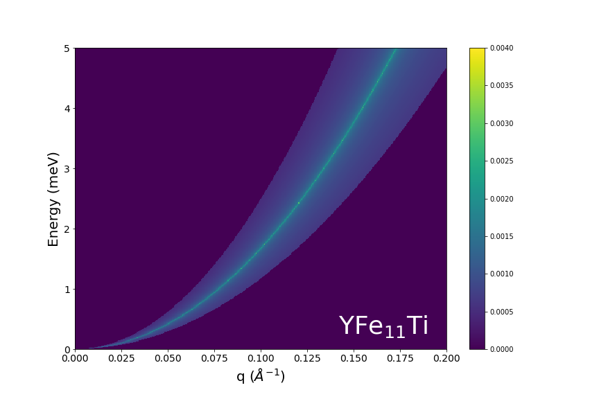
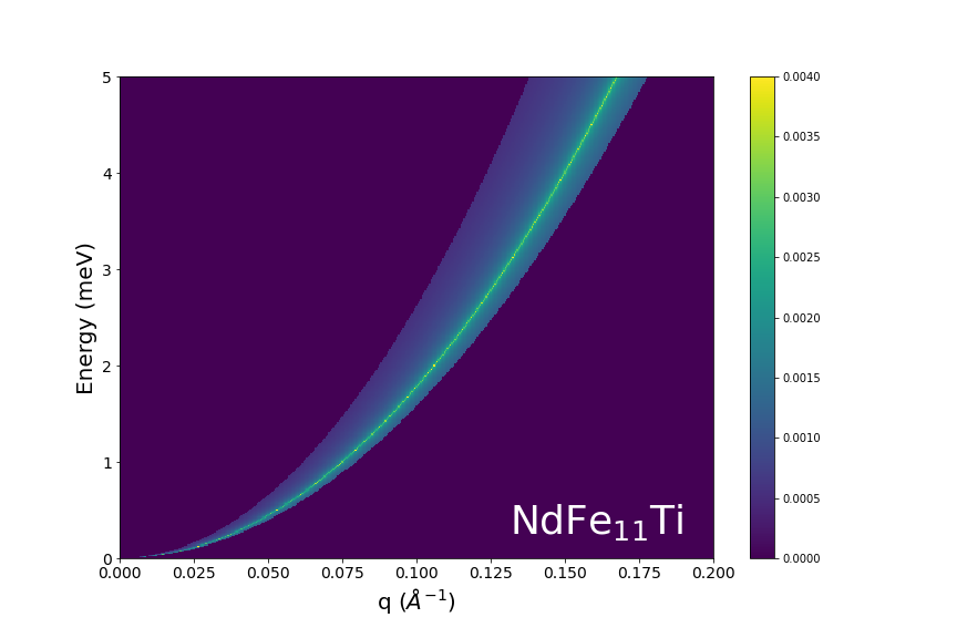
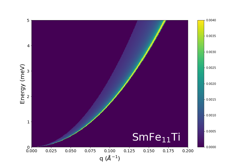
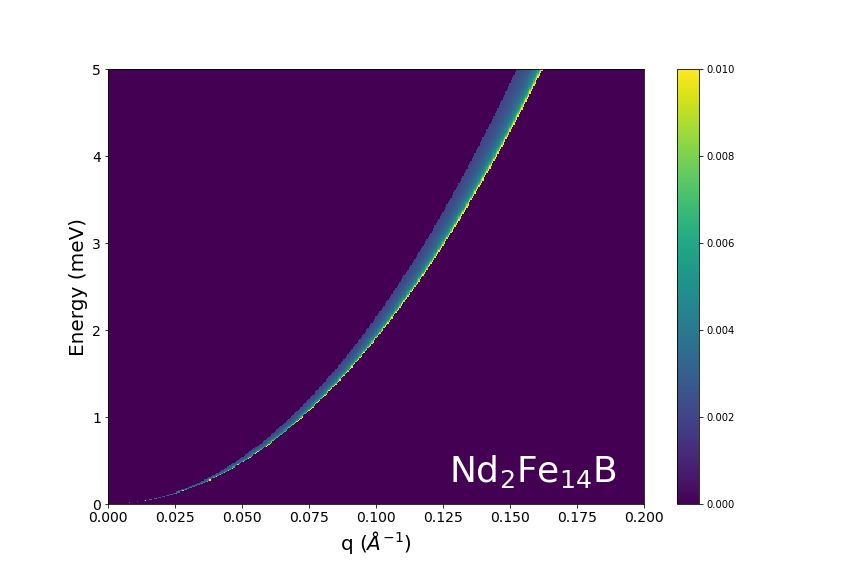
Figure 3: (Color online) Angular-integrated spin-wave dispersion for $R$Fe₁₁Ti and Nd₂Fe₁₄B. These color maps show the density of states $I(q,E)$ of Eq. (22) where the horizontal axis denotes the absolute value of a wave vector, $q$, and the vertical axis is the energy, $E$.

As mentioned in Appendix B, the lower edge of the finite-DOS region is given by $E=D_{\min}q^{2}$ and the upper edge by $E=D_{\max}q^{2}$, where $D_{\min}=\min(D_{a},D_{b},D_{c})$ and $D_{\max}=\max(D_{a},D_{b},D_{c})$. Therefore, the anisotropy of the spin-wave stiffness is reflected in the smearing of the dispersion in these figures. The smearing in Nd₂Fe₁₄B is much smaller than the measurement errors in the neutron scattering experiment by Ono et al.Ono et al. (2014). Hawai et al. recently performed inelastic neutron diffraction experiments for $R$Fe₁₁Ti.Hawai et al. Although anisotropy could not be seen in their data due to uncertainties in the experiment, further development of neutron scattering techniques will hopefully resolve the existence of the anisotropy.

IV Conclusion

We presented the spin-wave dispersion for Nd₂Fe₁₄B and $R$Fe₁₁Ti obtained using first-principles calculations. Our recently developed RSA, an accelerated scheme for spin-wave dispersion that is based on the Liechtenstein formula and its use in reciprocal space, enabled these calculations in practical time. We discuss the anisotropy of the exchange stiffness in Nd₂Fe₁₄B. Our results suggest that the anisotropy in the exchange stiffness of Nd₂Fe₁₄B is much smaller than the values obtained by previous Monte Carlo simulations. We also demonstrated that the spatial cutoff can be a crucial factor in the precision when estimating the anisotropy. However, $R$Fe₁₁Ti has a strong anisotropy in our estimation of the spin-wave stiffness. We also showed the angular integrated dispersion of the spin-waves, which corresponds to diffraction of polycrystalline and powder samples. We pointed out that the anisotropy can be seen as smearing of the $E$–$q$ dispersion, and this is comparable with neutron scattering experiments.

Appendix A Convergence with respect to the number of $k$ points in Fe and Co

We examine the convergence of the calculation for bcc-Fe and hcp-Co with respect to the number of $k$-points. Figure 4 shows the spin-wave dispersion obtained by our calculation. The solid lines are for the calculations with the largest number of $k$-points. The overall behavior of the curve agrees with previous studiesHalilov et al. (1998); Pajda et al. (2001). The dashed curves show the results with a smaller number of $k$-points, and the dash-dotted curves with an even smaller number.

In the case of Fe, we need a large number of $k$-points to reproduce the description of the spin-wave dispersion with $18\times 18\times 18$ $k$-points (solid). The dot-dashed curve shows the dispersion with $8\times 8\times 8$ $k$-points (dot-dashed), which is the cheapest calculation among the three and has a significant deviation from the solid curve. With $12\times 12\times 12$ $k$-points (dashed), some features such as the depth of the dip on the $\Gamma$–H line are missing. However, we confirmed that the curves with $14\times 14\times 14$ $k$-points appear much closer to the solid curve. In the case of Co, convergence is much faster owing to the smallness of the Brillouin zone, and $9\times 9\times 9$ $k$-points seem to be enough.

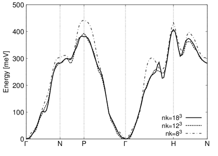
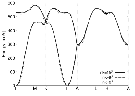
Figure 4: Spin-wave dispersion in (Top) bcc-Fe and (Bottom) hcp Co. The solid lines are from the calculations with the largest number of $k$-points (nk): $18\times 18\times 18$ for Fe; $15\times 15\times 15$ for Co. The dashed lines and the dash-dot lines are for smaller nk.

Figure 5 shows the convergence of the spin-wave stiffness—the curvature around the $\Gamma$ point in the lowest branch—with respect to the number of $k$-points. The filled circles show the results when the SCF potential was obtained with the same number of $k$-points as used in the spin-wave calculation. The spin-wave stiffness appears well-behaved as a function of the number of $k$-points and converges rapidly.

Figure 5: Convergence of the spin-wave stiffness with respect to the number of the $k$-points (nk) where nk for SCF is the same as the spin-wave calculation (filled circle), and where nk is fixed to 1000 (open circle). Note that the horizontal axis is in log scale.

We also show the results for the SCF potential fixed to that obtained with $10\times 10\times 10$ $k$-points as open circles. By comparison, we observe that the quality of the potential does not have much effect on the spin-wave stiffness.

Appendix B $E$–$q$ dispersion of spin-waves

To compare the theoretical results with experimental results for polycrystalline and powder samples, we perform angular integration of the following energy dispersion:

$$E=D_{a}q_{a}^{2}+D_{b}q_{b}^{2}+D_{c}q_{c}^{2}\quad(0\leq D_{a}\leq D_{b}\leq D_{c}),$$ (10)

which is adequate when the low-energy excitations are of interest. The inequality for the coefficients does not deteriorate the generality because it is always satisfied by exchanging the labels of axes.

It is obvious that there are states only when $D_{a}q^{2}\leq E\leq D_{c}q^{2}$ holds. We divide the problem into 3 cases: (i) $D_{a}q^{2}\leq E<D_{b}q^{2}$, (ii) $E=D_{b}q^{2}$, and (iii) $D_{b}q^{2}<E\leq D_{c}q^{2}$. In the case of (i), by eliminating $q_{a}^{2}$ in $E$ with $q_{a}^{2}=q^{2}-q_{b}^{2}-q_{c}^{2}$, we can obtain

$$\frac{x^{2}}{\alpha^{2}}+\frac{y^{2}}{\beta^{2}}=\epsilon^{2}\quad(0<\alpha\leq\beta),$$ (11)

$$z^{2}=q^{2}-x^{2}-y^{2},$$ (12)

with

$$\alpha=\sqrt{\frac{1}{D_{c}-D_{a}}},\quad\beta=\sqrt{\frac{1}{D_{b}-D_{a}}},\quad\epsilon=\sqrt{E-D_{a}q^{2}},$$ (13)

$$x=q_{c},\quad y=q_{b},\quad z=q_{a}.$$ (14)

In the case of (ii), we can immediately obtain

$$(D_{b}-D_{a})q_{a}^{2}=(D_{c}-D_{b})q_{c}^{2}$$ (15)

by eliminating $q_{b}$ in $E$. In the case of (iii), by eliminating $q_{c}^{2}$ in $E$ with $q_{c}^{2}=q^{2}-q_{a}^{2}-q_{b}^{2}$, we can obtain the same set of equations as Eq. (11) and Eq. (12) with

$$\alpha=\sqrt{\frac{1}{D_{c}-D_{a}}},\quad\beta=\sqrt{\frac{1}{D_{c}-D_{b}}},\quad\epsilon=\sqrt{D_{c}q^{2}-E},$$ (16)

$$x=q_{a},\quad y=q_{b},\quad z=q_{c}.$$ (17)

Therefore, we can express the equations for the possible sets of $q_{a},q_{b},q_{c}$ by a single set of equations—Eq. (11) and Eq. (12)—except for the singular point at which (ii) $E=D_{b}q^{2}$ holds.

When considering the density of states of spin-waves, we can disregard case (ii) because it has a measure of zero in the integral with respect to energy. Let us consider a solution $\vec{P}=(x,y,z)$ of (11) and (12) in the $z>0$ region. By the following transform:

$$x =\epsilon\alpha\cos\theta,$$ (18)

$$y =\epsilon\beta\sin\theta,$$ (19)

this vector can be expressed as follows:

$$\vec{P}=\left(\epsilon\alpha\cos\theta,\epsilon\beta\sin\theta,\sqrt{q^{2}-\epsilon^{2}(\alpha^{2}\cos^{2}\theta+\beta^{2}\sin^{2}\theta)}\right).$$ (20)

When $\Delta E$ and $\Delta q$ are infinitesimal numbers, the number of states within the energy range from $E$ to $E+\Delta E$ and within the momentum range from $q$ to $q+\Delta q$ can be expressed as

$$I(q,E)\Delta E\Delta q=\frac{2V}{8\pi^{3}}\int^{\pi}_{-\pi}d\theta\left|\frac{\partial(x,y,z)}{\partial(q,E,\theta)}\right|\Delta E\Delta q$$ (21)

where $V$ denotes the system volume. The factor of two is necessary because there is another solution $(x,y,-z)$ in $z<0$. By straightforward calculation, we can obtain an expression with the complete elliptic integral of the first kind, $K(k)$, as follows:

$$I(q,E)=\frac{V}{\pi^{3}}\,\alpha\beta\frac{q}{\sqrt{q^{2}-\epsilon^{2}\alpha^{2}}}\,K\left(\sqrt{\frac{(\beta^{2}-\alpha^{2})\epsilon^{2}}{q^{2}-\epsilon^{2}\alpha^{2}}}\right),$$ (22)

An outline of this is shown in Fig. 6. Although we can also write the elliptic modulus, $k=\sqrt{{(\beta^{2}-\alpha^{2})\epsilon^{2}}/{(q^{2}-\epsilon^{2}\alpha^{2})}}$, in terms of the variables in Eq. (10), the expressions for cases (i) and (iii) are different:

$$k^{2} ={(\beta^{2}-\alpha^{2})\epsilon^{2}}/{(q^{2}-\epsilon^{2}\alpha^{2})}$$

$$=\begin{dcases}\frac{D_{c}-D_{b}}{D_{c}q^{2}-E}\frac{E-D_{a}q^{2}}{D_{b}-D_{a}}&\text{Case (i)}\\ \frac{D_{b}-D_{a}}{E-D_{a}q^{2}}\frac{D_{c}q^{2}-E}{D_{c}-D_{b}}&\text{Case (iii)}\end{dcases},$$ (23)

with which one can observe $0\leq k^{2}<1$. When $E$ is fixed, $k$ is a monotonically increasing function of $q$ in case (i) while $k$ is monotonically decreasing in case (iii). Because $K(k)$ is also a monotonically increasing function, we observe

$$I(E)\leq\lim_{E\rightarrow D_{b}q^{2}}I(E)=I(D_{b}q^{2}).$$ (24)

Therefore, the density of states is most intense along the line of $E=D_{b}q^{2}$.

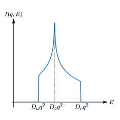
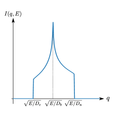
Figure 6: Outlines of $I(q,E)$ in Eq. (22) where (Left) $q$ is fixed and (Right) $E$ is fixed.

References

- Hirayama et al. (2017) Y Hirayama, Y K Takahashi, S Hirosawa, and K Hono, “Intrinsic hard magnetic properties of Sm(Fe1-xCox)12 compound with the ThMn12 structure,” Scripta Materialia 138, 62–65 (2017).
- Mayer et al. (1991) HM Mayer, M Steiner, N Stüer, H Weinfurter, K Kakurai, B Dorner, Per-Anker Lindgård, KN Clausen, S Hock, and W Rodewald, “Inelastic neutron scattering measurements on Nd2Fe14B single crystals,” Journal of magnetism and magnetic materials 97, 210–218 (1991).
- Mayer et al. (1992) HM Mayer, M Steiner, N Stüer, H Weinfurter, B Dorner, Per-Anker Lindgård, KN Clausen, S Hock, and R Verhoef, “Inelastic neutron scattering measurements on Nd2Fe14B and Y2Fe14B single crystals,” Journal of Magnetism and Magnetic Materials 104, 1295–1297 (1992).
- Ono et al. (2014) K Ono, N Inami, K Saito, Y Takeichi, M Yano, T Shoji, A Manabe, A Kato, Y Kaneko, D Kawana, et al., “Observation of spin-wave dispersion in Nd-Fe-B magnets using neutron Brillouin scattering,” Journal of Applied Physics 115, 17A714 (2014).
- Naser et al. (2020) H Naser, C Rado, G Lapertot, and S Raymond, “Anisotropy and temperature dependence of the spin-wave stiffness in nd 2 fe 14 b: An inelastic neutron scattering investigation,” Physical Review B 102, 014443 (2020).
- Toga et al. (2018) Yuta Toga, Masamichi Nishino, Seiji Miyashita, Takashi Miyake, and Akimasa Sakuma, “Anisotropy of exchange stiffness based on atomic-scale magnetic properties in the rare-earth permanent magnet nd 2 fe 14 b,” Physical Review B 98, 054418 (2018).
- Gong et al. (2019) Qihua Gong, Min Yi, Richard F. L. Evans, Bai-Xiang Xu, and Oliver Gutfleisch, “Calculating temperature-dependent properties of permanent magnets by atomistic spin model simulations,” Phys. Rev. B 99, 214409 (2019).
- Gong et al. (2020) Qihua Gong, Min Yi, Richard F. L. Evans, Oliver Gutfleisch, and Bai-Xiang Xu, “Anisotropic exchange in Nd–Fe–B permanent magnets,” Materials Research Letters 8, 89–96 (2020), https://doi.org/10.1080/21663831.2019.1702116 .
- Halilov et al. (1998) S V Halilov, H Eschrig, A Y Perlov, and P M Oppeneer, “Adiabatic spin dynamics from spin-density-functional theory: Application to Fe, Co, and Ni,” Physical Review B 58, 293 (1998).
- Van Schilfgaarde and Antropov (1999) M Van Schilfgaarde and VP Antropov, “First-principles exchange interactions in fe, ni, and co,” Journal of applied physics 85, 4827–4829 (1999).
- Shallcross et al. (2005) S. Shallcross, A. E. Kissavos, V. Meded, and A. V. Ruban, “An ab initio effective hamiltonian for magnetism including longitudinal spin fluctuations,” Phys. Rev. B 72, 104437 (2005).
- Yu et al. (2008) P. Yu, X. F. Jin, J. Kudrnovský, D. S. Wang, and P. Bruno, “Curie temperatures of fcc and bcc nickel and permalloy: Supercell and green’s function methods,” Phys. Rev. B 77, 054431 (2008).
- Oguchi et al. (1983) T. Oguchi, K. Terakura, and A. R. Williams, “Band theory of the magnetic interaction in mno, mns, and nio,” Phys. Rev. B 28, 6443–6452 (1983).
- Liechtenstein et al. (1987) A I Liechtenstein, M I Katsnelson, V P Antropov, and V A Gubanov, “Local spin density functional approach to the theory of exchange interactions in ferromagnetic metals and alloys,” Journal of Magnetism and Magnetic Materials 67, 65–74 (1987).
- Mryasov et al. (1996) ON Mryasov, Arthur J Freeman, and AI Liechtenstein, “Theory of non-heisenberg exchange: Results for localized and itinerant magnets,” Journal of applied physics 79, 4805–4807 (1996).
- Pajda et al. (2001) Marek Pajda, J Kudrnovskỳ, I Turek, Vaclav Drchal, and Patrick Bruno, “Ab initio calculations of exchange interactions, spin-wave stiffness constants, and Curie temperatures of Fe, Co, and Ni,” Physical Review B 64, 174402 (2001).
- Šipr et al. (2019) O. Šipr, S. Mankovsky, and H. Ebert, “Spin wave stiffness and exchange stiffness of doped permalloy via ab initio calculations,” Phys. Rev. B 100, 024435 (2019).
- Okumura et al. (2019) H Okumura, K Sato, and T Kotani, “Spin-wave dispersion of 3 d ferromagnets based on quasiparticle self-consistent g w calculations,” Physical Review B 100, 054419 (2019).
- Fukazawa et al. (2019) Taro Fukazawa, Hisazumi Akai, Yosuke Harashima, and Takashi Miyake, “First-principles study of spin-wave dispersion in Sm(Fe1-xCox)12,” Journal of Magnetism and Magnetic Materials 469, 296–301 (2019).
- Hohenberg and Kohn (1964) Pierre Hohenberg and Walter Kohn, “Inhomogeneous electron gas,” Physical Review 136, B864 (1964).
- Kohn and Sham (1965) Walter Kohn and Lu Jeu Sham, “Self-consistent equations including exchange and correlation effects,” Physical Review 140, A1133 (1965).
- Perdew and Zunger (1981) J. P. Perdew and Alex Zunger, “Self-interaction correction to density-functional approximations for many-electron systems,” Phys. Rev. B 23, 5048–5079 (1981).
- Tatetsu et al. (2018) Yasutomi Tatetsu, Yosuke Harashima, Takashi Miyake, and Yoshihiro Gohda, “Role of typical elements in (, C, N, O, F),” Phys. Rev. Materials 2, 074410 (2018).
- Harashima et al. (2015) Yosuke Harashima, Kiyoyuki Terakura, Hiori Kino, Shoji Ishibashi, and Takashi Miyake, “First-principles study of structural and magnetic properties of R(Fe,Ti)12 and R(Fe,Ti)12N (R= Nd, Sm, Y),” in Proceedings of Computational Science Workshop 2014 (CSW2014), JPS Conference Proceedings, Vol. 5 (2015) p. 1021.
- (25) Takafumi Hawai, Masao Yano, Tetsuya Shoji, Hiraku Saito, Tetsuya Yokoo, Shinichi Itoh, and Kanta Ono, “Spin-wave for material design of rare-earth magnets,” private communication.