IMPULSIVELY GENERATED SAUSAGE WAVES IN CORONAL TUBES WITH TRANSVERSALLY CONTINUOUS STRUCTURING
Abstract
The frequency dependence of the longitudinal group speeds of trapped sausage waves plays an important role in determining impulsively generated wave trains, which have often been invoked to account for quasi-periodic signals in coronal loops. We examine how the group speeds () depend on angular frequency () for sausage modes in pressureless coronal tubes with continuous transverse density distributions by solving the dispersion relation pertinent to the case where the density inhomogeneity of arbitrary form takes place in a transition layer of arbitrary thickness. We find that in addition to the transverse lengthscale and density contrast , the group speed behavior depends also on the detailed form of the density inhomogeneity. For parabolic profiles, always decreases with first before increasing again, as happens for the much studied top-hat profiles. For linear profiles, however, the behavior of the curves is more complex. When , the curves become monotonical for large values of . On the other hand, for higher density contrasts, a local maximum exists in addition to a local minimum when coronal tubes are diffuse. With time-dependent computations, we show that the different behavior of group speed curves, the characteristic speeds and in particular, is reflected in the temporal evolution and Morlet spectra of impulsively generated wave trains. We conclude that the observed quasi-periodic wave trains not only can be employed to probe such key parameters as density contrasts and profile steepness, but also have the potential to discriminate between the unknown forms of the transverse density distribution.
1 INTRODUCTION
The past two decades have seen rapid progress in the field of solar magneto-seismology (SMS, for recent reviews, see e.g., Nakariakov & Verwichte 2005; Banerjee et al. 2007; De Moortel & Nakariakov 2012; Wang 2016; Nakariakov et al. 2016). Among the rich variety of the low-frequency waves observed in the Sun’s atmosphere, flare-related quasi-periodic fast propagating (QFP) wave trains have received much attention (see Liu & Ofman 2014, for a recent review). Their quasi-periods usually ranging from to secs, these wave trains were discovered (Liu et al. 2011) and extensively observed in images acquired with the Atmospheric Imaging Assembly on board the Solar Dynamics Observatory (SDO/AIA, Liu et al. 2012; Yuan et al. 2013; Shen et al. 2013; Nisticò et al. 2014; also see Lemen et al. 2012 for the description of the instrument). On the other hand, quasi-periodic signals in coronal emissions presumably from density-enhanced loops have been known since the 1960’s (e.g., Parks & Winckler 1969, Frost 1969, Rosenberg 1970, McLean & Sheridan 1973; see Table 1 of Aschwanden et al. 1999 for a comprehensive compilation of measurements prior to 2000). The quasi-periods of a considerable fraction of these signals were of the order of seconds. While these measurements were largely spatially unresolved, more recent high-cadence instruments imaging the corona at total eclipses also indicated the presence in coronal loops of quasi-periodic signals both with seconds (Williams et al. 2001, 2002; Katsiyannis et al. 2003) and with seconds (Samanta et al. 2016). In addition, quasi-periodic pulsations (QPPs) in the lightcurves of solar flares with similar periods have also been measured using imaging instruments such as the Nobeyama Radioheliograph (NoRH, e.g., Asai et al. 2001; Nakariakov et al. 2003; Melnikov et al. 2005; Kupriyanova et al. 2013), SDO/AIA (e.g., Su et al. 2012), and more recently with the Interface Region Imaging Spectrograph (IRIS, Tian et al. 2016; see also De Pontieu et al. 2014 for the description of IRIS).
Interestingly, quasi-periodic waves are not necessarily connected to quasi-periodic activities of the sources but can also be attributed to their impulsive generation (see Jiao et al. 2015 and Samanta et al. 2015 for recent observational evidence, Yang et al. 2015 and Yuan et al. 2016 for numerical demonstrations). As explained by Roberts et al. (1983, 1984), the key here is wave dispersion. For simplicity, consider fast sausage waves in a density-enhanced coronal loop where the transverse density distribution is in a top-hat fashion, characterized by the internal () and external values (). Let and denote the internal and external Alfvén speeds, respectively (). It is well-known that two regimes exist for sausage waves, depending on how the axial wavenumber compares with some critical value . The leaky regime arises when , whereby waves lose their energy by radiating fast waves into the surroundings (Meerson et al. 1978; Spruit 1982; Cally 1986). When , however, the trapped regime results and wave energy is well confined to coronal loops. Trapped sausage waves are substantially dispersive such that when the angular frequency increases from , the axial group speed first decreases to a local minimum at , before increasing towards . Graphically speaking, this means that the curve comprises two portions: in one portion a horizontal line representing a constant intersects the curve at a single point (), whereas multiple intersections exist in the other (). Let the first (second) portion be labeled “S” (“M”), short for “single” (“multiple”). Roberts et al. (1984) predicted that in response to an impulsive internal axisymmetric source, the signal in the loop at a distance sufficiently far away comprises three phases (see also Edwin & Roberts 1986, for a heuristic discussion). For the time interval , wavepackets in portion S are relevant and individual wavepackets with progressively low group speeds arrive consecutively. Portion M then becomes relevant when , whereby multiple wavepackets with the same group speed but different frequencies arrive simultaneously. The signal now is expected to be stronger than in the first phase due to the superposition of multiple wavepackets. When , no incoming wavepackets are expected, resulting in some decaying signal oscillating at an angular frequency . These three phases are traditionally termed the periodic, quasi-periodic and decay (or Airy) phases.
The theoretically expected evolution of impulsively generated sausage waves has been shown to be robust by both analytical and numerical studies. Examining the response of a transversally discontinuous coronal tube to localized, axisymmetric, footpoint motions, Berghmans et al. (1996) showed analytically that an alternative interpretation of the periodic phase is that wavefronts that initially leak out of the tube will return back in view of the continuity of the transverse Lagrangian displacement. Also examining coronal tubes with top-hat transverse density profiles, the more recent analytical study by Oliver et al. (2015) showed that impulsively generated waves can be examined in terms of the partition of the energy contained in the initial perturbation between proper and improper modes. On the other hand, impulsively generated sausage waves have also been numerically examined in both coronal slabs (Murawski & Roberts 1993, 1994; Nakariakov et al. 2004; Pascoe et al. 2013; Yu et al. 2016b) and coronal tubes (Selwa et al. 2007; Shestov et al. 2015), for which the density is transversally distributed in a continuous manner. What these studies suggest is that, while such factors as the axial extent of the initial perturbation (Oliver et al. 2015) and density profile steepness (Nakariakov et al. 2004; Shestov et al. 2015) are important, impulsively generated wave trains can still to a large extent be understood in the framework proposed by Roberts et al. (1984). In particular, the numerical studies by Nakariakov et al. (2004) and Shestov et al. (2015) showed that the period and amplitude modulations in the wave trains transform into tadpole-shaped Morlet spectra. This spectral feature was actually seen in both radio (e.g., Jelinek & Karlicky 2010; Karlický et al. 2013) and optical measurements (e.g., Katsiyannis et al. 2003; Samanta et al. 2016).
The temporal and wavelet features of impulsively generated waves can help yield such key information as the internal Alfvén speed, density contrast between loops and their surroundings, as well as the location of the source (e.g., Roberts et al. 1984; Roberts 2008). However, such applications are primarily based on the theoretical results for fast sausage waves in coronal tubes with a top-hat transverse density profile (Edwin & Roberts 1983). While theoretical results are known for a limited number of continuous density profiles, they are either not fully developed (Edwin & Roberts 1988) or have not been applied to the context of impulsively generated waves (Lopin & Nagorny 2014, 2015). In an effort of developing a more general theory for sausage waves, we worked in the framework of cold MHD and examined coronal tubes with transverse density profiles that comprise a uniform cord, an external uniform medium, and a transition layer (TL) connecting the two (Chen et al. 2015, hereafter Paper I). The TL can be of arbitrary width and the density profile therein can be of arbitrary form. We further showed that it is straightforward to eliminate the requirement for the density profile to involve a uniform cord (Guo et al. 2016). The present manuscript intends to make a fuller use of the theory developed in Paper I, and to examine how different prescriptions for the transverse density profiles influence the properties of impulsively generated sausage waves.
This manuscript is organized as follows. Section 2 extends some previous theoretical studies on sausage waves in coronal tubes with two simple density profiles. The purpose is to offer some new analytical results such that the the frequency dependence of the group speeds can be better understood. Section 3 builds on our Paper I and provides a detailed examination on how different profile choices impact the group speed curves. The consequences on the temporal evolution of impulsively generated waves are also discussed therein with the aid of time-dependent computations. Finally, Section 4 closes this manuscript with our summary and some concluding remarks.
2 SAUSAGE WAVES IN CORONAL LOOPS WITH TWO SIMPLE DENSITY PROFILES
In view of applications to the solar corona where gas pressure is usually much smaller than magnetic pressure, we adopt the cold MHD description in which the gas to magnetic pressure ratio is taken to be zero. We model coronal loops as straight magnetic tubes with a mean radius and directed in the -direction in a cylindrical coordinate system . The magnetic field is uniform and also in the -direction, . We proceed with a standard eigenmode analysis by assuming that all perturbations are proportional to . Note that both and are taken to be real, given that only trapped modes are of interest here. In addition, only the lowest-order sausage waves will be examined throughout.
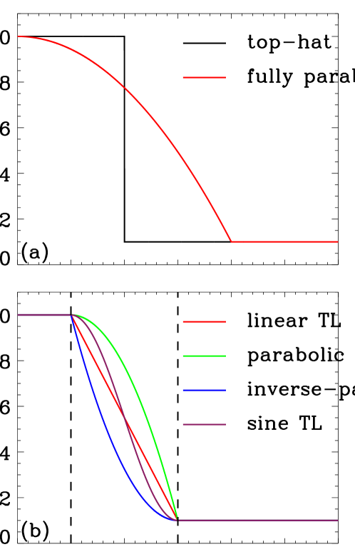
As stated in the introduction, this study will be focused on the effects of different transverse density profiles on impulsively generated sausage waves. However, it is evidently impossible to exhaust all possible choices for the largely unknown form of density distribution. We therefore choose to examine a set of profiles that are often invoked in examinations of kink modes (e.g., Ruderman & Roberts 2002; Van Doorsselaere et al. 2004; Soler et al. 2014). Figure 1 displays the chosen profiles where for illustration purposes, a value of is adopted for the density contrast , the ratio of the density at the loop axis to that far from the loop. The profiles in Figure 1b pertains to Section 3 and will be explained therein. This section will examine the two profiles in Figure 1a where they are labeled “top-hat” and “fully parabolic”. As will be shown, compact closed-form expressions can be found for sausage waves in coronal loops with these two simple profiles.
2.1 Top-hat Profiles
Let us start with a top-hat transverse density profile (illustrated by the black curve in Figure 1a),
| (3) |
where the subscripts and denote the internal and external values, respectively. The dispersion relation (DR) for trapped sausage waves reads (e.g., Edwin & Roberts 1983)
| (4) |
where () represents Bessel function of the first kind (modified Bessel function of the second kind) with . In addition,
| (5) |
in which is the Alfvén speed. To proceed, let and denote the axial phase and group speeds, respectively.
2.2 Fully Parabolic Profiles
Now consider a continuous density profile given by
| (10) |
where denotes the loop-external-medium interface, with being the mean tube radius. For future reference, let this profile be denoted by “fully parabolic”, which is illustrated by the red curve in Figure 1a. A similar profile was considered by Pneuman (1965), where the external medium was taken to be vacuum (). Omitting the details, we extend the mathematical procedure therein to account for a finite , with the resulting DR reading
| (11) |
where
In addition,
is Kummer’s function. When deriving Equation (11), we have used the fact that
Approximate expressions for and at large can also be found by generalizing the results of Pneuman (1965) where . For the lowest order sausage waves, we find that rapidly approaches zero with increasing . Consequently,
| (12) |
and
| (13) |
As in the top-hat case, one expects to see that () approaches from above (below).
2.3 Group Speed Curves
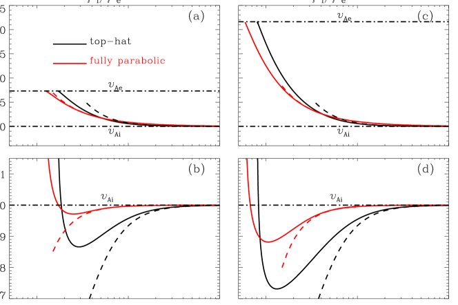
Figure 2 presents the dependence of the phase (the upper row) and group (lower) speeds for both a top-hat (the black curves) and a fully parabolic (red) profile. For illustration purposes, two values, (the left column) and (right), are adopted for the density ratio . In addition to the full numerical solutions to the DRs (the solid lines), we also plot their approximate expressions for large axial wavenumbers (dashed). From Figures 2a and 2c one sees that for both profiles, trapped waves exist only when exceeds some critical value , beyond which decreases monotonically with and approaches as expected. In addition, one sees that for both density contrasts, the dimensionless critical wavenumber is smaller for the fully parabolic than for the top-hat profile. Actually this is true for in an extensive range between and . As for the group speeds, one sees from Figures 2b and 2d that decreases sharply first with before increasing towards for large . The asymptotic dependence of both and for the fully parabolic profile is well approximated by the analytical expressions (12) and (13). For instance, when , the red dashed lines can hardly be told apart from the solid ones when . For the top-hat profiles, however, one sees that the black dashed curves converge to the solid ones only for sufficiently large . When , this happens for . The reason for the different performance of the approximate expressions at large is that the density contrast does not appear in Equations (6) and (7) for top-hat profiles, whereas it is explicitly involved for fully parabolic profiles (see Equations 12 and 13).
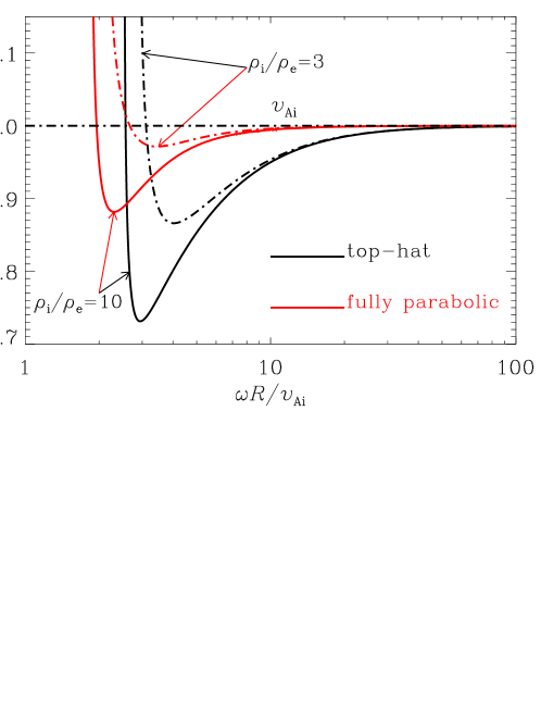
The wavenumber dependence is readily translated into frequency dependence, which is displayed in Figure 3. Once again two different density contrasts, (the dash-dotted curves) and (solid) are shown for illustration purposes. One sees the typical behavior for to posses a local minimum . This behavior is well-known for top-hat profiles (Roberts et al. 1983, 1984), and from Equation (7) we know that this dependence of the group speed curves holds regardless of the density contrast, even though only two values are examined here. However, the group speed curves for fully parabolic profiles are qualitatively different from the only relevant study where was shown to increase monotonically with from zero to when (Pneuman 1965, Figure 2). In this regard, the red curves in Figure 3 show that a finite , or physically speaking the finite elasticity of the external medium, is crucial for to posses a local minimum (see also the discussion in Edwin & Roberts 1988, Section 3.2). In addition, the asymptotic expression (13) indicates that such a local minimum exists for arbitrary , as long as it is finite.
3 SAUSAGE WAVES IN CORONAL TUBES WITH ARBITRARY DENSITY PROFILES
At this point, we note that both top-hat and fully parabolic profiles lead to the classical group speed curves possessing a local minimum, and this behavior holds for arbitrary density contrasts as long as the external density does not vanish. Let () denote the tendency for to increase (decrease) with . Then typically one sees this behavior. However, will other possibilities appear for some other density profiles? This is addressed in the present section.
3.1 Profile Description and Dispersion Relation
We choose to examine some density profiles adopted in Paper I, where the transverse density distribution comprises a transition layer (TL) of width connecting a uniform cord and a uniform external medium,
| (17) |
The profile between is such that the equilibrium density decreases continuously from the internal value to the external one . Evidently, the thickness of this TL (), a measure of profile steepness, is bounded by and . In this sense, the dimensionless parameter can be used to distinguish between thin (with, say, ) and thick (with ) transition layers. Two prescriptions will be explored here,
| (20) |
For an illustration of these two profiles, please see Figure 1b where and are arbitrarily chosen to be and , respectively. We note that the profile labeled “parabolic TL” recovers the fully parabolic profile (10) when approaches .
The DR for sausage waves for arbitrary prescriptions of in a TL of arbitrary thickness was given by Equation (17) in Paper I. Focusing on trapped waves, one can readily reformulate this DR as
| (21) |
Here and have already been defined by Equation (5). In addition, and . Furthermore, and denote two linearly independent solutions for the Lagrangian displacement in the TL. Both are expressed as a regular series expansion around ,
Without loss of generality, we choose
The rest of the coefficients and are given by Equation (11) in paper I, and contain the information on the density distribution. Furthermore, the prime ′ denotes the derivative of with respect to .
3.2 Group Speed Curves
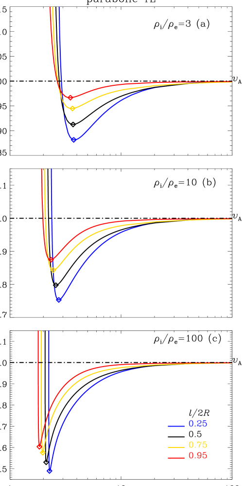
Let us first examine parabolic TL profiles, which approach top-hat profiles when , and approach fully parabolic profiles when . Now that for these two extremes the group speed curves are both of the classical type, one expects that the frequency dependence of will not be qualitatively different when varies between and . Figure 4 shows that this is indeed the case: for a number of arbitrarily chosen and , always first sharply decreases with before increasing towards . Furthermore, one sees that the group speed curves in the portion before reaching the local minima (where ) become increasingly steep when increases. This happens because gets increasingly close to the angular frequency () at the cutoff wavenumber. Take for instance. It turns out that when (), () and () (here and hereafter in units of ). For comparison, reads when , in which case is found to be .
The group speed behavior is further examined in Figure 5 where (a) the minimum group speed () and (b) the angular frequency at which this minimum is attained () are shown by equally spaced contours in the space spanned by and . One sees from Figure 5a that at a given density contrast, tends to increase with , while it decreases with when is fixed. Examining Figure 5b, one sees that while tends to decrease with at a fixed , its dependence on is different at different values of . For , hardly varies with . However, for larger density contrasts, tends to decrease with , with the tendency becoming increasingly prominent when increases. We note by passing that for typical active region loops, the density contrast tends to lie between and (e.g., Aschwanden et al. 2004). Furthermore, density contrasts as large as are not unrealistic but have been observationally deduced for, say, prominences (e.g., Patsourakos & Vial 2002; Labrosse et al. 2010).
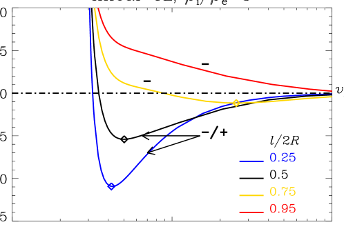
How about linear TL profiles? Figure 6 displays the dependence of for a number of as given by the curves in different colors. Here a rather modest density ratio of is chosen. Comparing the blue and black curves corresponding to and , respectively, one sees that , the angular frequency where the group speed attains its minimum, increases when the density profile becomes more diffuse. In fact, when (the red curve), moves out to infinity, and hence the “” label. We note that for coronal slabs with transverse density distributions describable by the generalized Epstein profile, Edwin & Roberts (1988, Figure 2) and Nakariakov & Roberts (1995) showed that the group speed curves also experience a transition from the “” to the “” type when the density profile becomes less steep than the symmetric Epstein one. What is interesting here is that, the existence of this transition depends not only on the profile steepness (or equivalently, the transverse lengthscale), but also on how the density distribution is described. When parabolic TL profiles are adopted, Figure 5 indicates that the group speed curves are exclusively of the “” type. It is necessary to point out that, when , the group speed curve in yellow is labeled with a “” symbol despite that it does attain a minimum. The reason is that, this minimum is smaller than by no more than and is attained at some rather large frequency. In fact, is as large as in this case. As will be demonstrated by further time-dependent computations (see Figure 13), the temporal evolution of impulsively generated sausage waves pertinent to this combination of parameters closely resembles the case where a local minimum is absent.
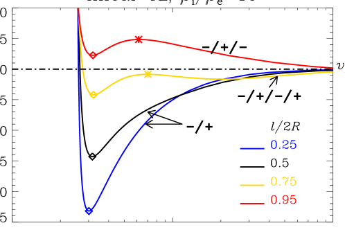
More complications arise for higher density contrasts, as shown by Figure 7 where . In addition to the “” behavior (see e.g., the case where ), can also behave in a “” () or a “” () manner. Evidently, these “” and “” cases are characterized by the existence of a local maximum attained at some , marked by the asterisks. Note that the case labeled “” possesses a second local minimum whose value lies between and the first minimum. In what follows, by “minimum” we always refer to the first local minimum wherever applicable.
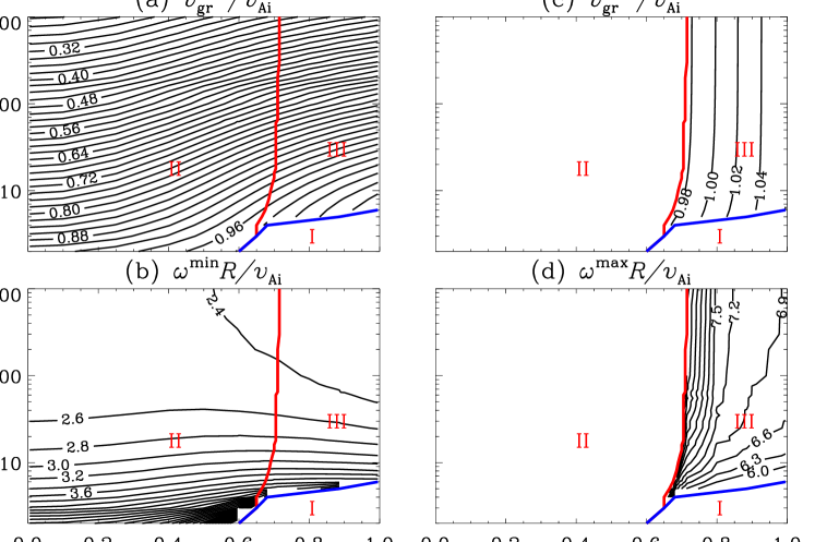
Figure 8 displays the distribution in the space of some parameters characterizing the group speed curves. The left (right) column concerns the first minimum (maximum). The red and blue curves represent the boundaries separating different types of group speed curves, and roughly divide this parameter space into three regions. The ones marked I, II, and III correspond to the cases where the group speed curves possess no extremum, one minimum, and more than one extrema. Note that in region I, for combinations of adjacent to the left border, the group speed curves look similar to the yellow curve in Figure 6, meaning that a local minimum does exist. However, in these cases the minima are exclusively less than by no more than , and further time-dependent computations indicate that the corresponding impulsively generated waves behave as if the minima were absent.
Examine the left column first. Figure 8a suggests that increases with but decreases with . On the other hand, from Figure 8b one sees that for low density contrasts with , increases with and a tiny increase in tends to lead to an extremely rapid increase in when the blue curve is approached from left (note the extremely closely packed contours there). In addition, one sees that in the region labeled III, tends to decrease with , even though this tendency is discernible only when . Now consider the right column. One sees from Figure 8c that tends to increase with but shows little dependence on . Furthermore, Figure 8d indicates that tends to decrease with but increase with .
3.3 Temporal Evolution of Impulsively Generated Sausage Waves
The analytical and numerical results presented in the previous sections suggest that the behavior of the group speed curves is qualitatively different with different prescriptions of the density distribution. However, one may question whether these characteristics can indeed be reflected in the temporal and wavelet signatures of impulsively generated waves. Before examining this, let us bear in mind that the temporal evolution of impulsively generated waves is sensitive not only to behavior of the group speed curves, but also relies on the details of the imposed initial perturbation (Oliver et al. 2015; Shestov et al. 2015). Let us further recall that according to Edwin & Roberts (1986), one way for characterizing the curve is to distinguish between the S and M portions, for which a horizontal line representing a constant intersects the curve at one point (multiple points). For the classical “” type, portion M is relevant when , the superposition of multiple wavepackets therein making the signal stronger than in the earlier stage. Actually the “” case is similar in the sense that the M portion also corresponds to , the only difference being that here should be interpreted as the first local minimum (e.g., the yellow curve in Figure 7). Let us consider what happens for the “” type, for which (e.g., the red curve in Figure 7). Now that the onset of portion M corresponds to a group speed of , one expects that plays a role in regulating the amplitude modulation. Likewise, for the monotical “” type (e.g., the red curve in Figure 6), one expects that the decay phase will not occur given the absence of a local extremum. In this regard, one way to bring out the influence of different types of group speed curves is to examine whether the corresponding characteristic speeds can be discerned in the impulsively generated wave trains.
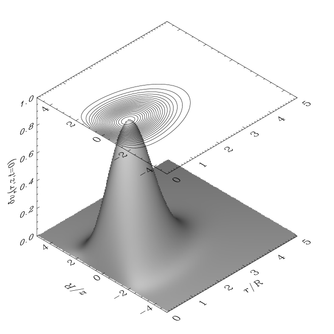
We now examine how pressureless coronal tubes respond to an impulsive, localized, axisymmetric source. To this end, we developed a simple finite-difference code, second order accurate in both space and time, to solve the aximmetrical version of linearized ideal MHD equations in the plane. The computational domain extends from to in the radial (transverse) direction, and from to in the axial (longitudinal) direction. The boundaries and are placed sufficiently far such that they are irrelevant in determining the perturbations. On the other hand, the boundary condition at the tube axis is specified in accordance with the parity of sausage modes. We specify the equilibrium density profile according to Equation (17). To initiate our computations, an initial perturbation is applied only to the transverse velocity around the origin, namely,
| (22) |
This initial perturbation is similar in form to what was adopted in Shestov et al. (2015), and ensures the parity of the generated wave trains by not displacing the loop axis. Furthermore, a constant is introduced such that the right-hand side attains a maximum of unity. Here and determine the extent to which the initial perturbation spans in the transverse and longitudinal directions, respectively. To make sure that primarily the lowest-order modes are excited, and are both chosen to equal , with the corresponding spatial profile of the initial perturbation shown in Figure 9. The details of our numerical code will be presented elsewhere, here it suffices to say that it has been validated via an extensive set of test problems, including computations of both standing and propagating modes. In addition, adopting a finer grid does not introduce any discernible difference to our computational results.
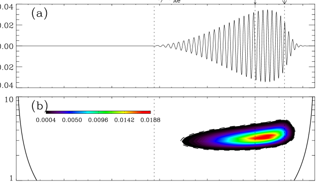
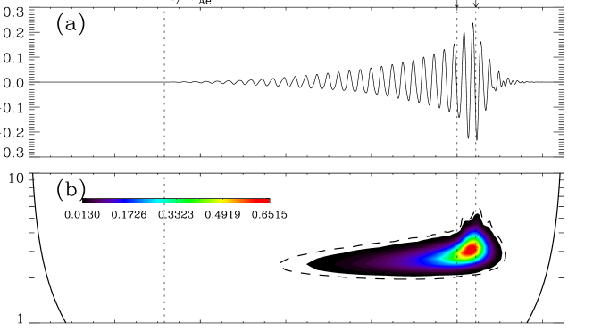
Let us start with an examination of the linear transition layer profile, and choose a combination of such that the group speed curve belongs to the “” type. Figure 10 displays (a) the temporal evolution and (b) the corresponding Morlet spectrum of the density perturbation sampled at a distance along the tube axis. This spectrum is created by using the standard wavelet toolkit devised by Torrence & Compo (1998). Note that the vertical axis in Figure 10b corresponds to angular frequency, and the black solid curve represents the cone of influence. In addition, the dashed contour represents the confidence level, computed by assuming a white-noise process for calculating the mean background spectrum (see section 4 in Torrence & Compo 1998). The dotted vertical lines correspond to the arrival times of wavepackets traveling at the internal () and external () Alfvén speeds as well as the local minimum (see the blue curve in Figure 6). In agreement with the reasoning by Edwin & Roberts (1986), one sees that the onset of the most significant power almost coincides with , which marks the start of the M portion of the group speed curve. Furthermore, the interval with strong power almost ends at , beyond which the signal evolves into the decay phase as expected. One can also see that the Morlet power for shows only a rather insignificant increase in frequency with time, the reason being that in this time interval the arriving wavepackets (with group speeds between and ) correspond to a rather narrow frequency range. When , the tendency for the Morlet power to increase with time is more obvious due to the arrival and superposition of wavepackets of higher frequencies (see the blue curve in Figure 6). In fact, the frequency modulation in the Morlet power spectra to be presented can all be understood from the behavior of the corresponding group speed curves.
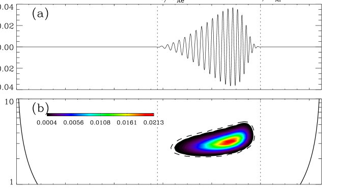
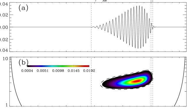
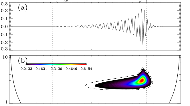
Still examining a linear transition layer profile with , Figure 11 shows what happens when the “” type arises by choosing to be . In this case, only and are relevant. One sees that marks the end of virtually any Morelet power, in agreement with the expectation that the decay phase will not be present due to the absence of a local minimum in the corresponding group speed curve. However, one may have noticed that for the parabolic transition layer profile with the same parameters, the group speed curve is not remarkably different in that the minimum is not too far from (actually , see the red curve in Figure 4a). The dispersion pertinent to is not significant, and one may see the group speed curve as being monotonically decreasing, as is the case for the relevant linear profile. One may then ask whether it is possible to discern this subtle difference between the linear and parabolic profiles. To address this, Figure 12 examines the pertinent parabolic case, from which one sees that indeed shows up by marking the end of the most significant Morlet power. In addition, now the decay phase is present due to the existence of , despite that it is indeed very close to . Another case that needs to be contrasted here is the linear transition layer profile with and . As shown by Figure 13, one sees that in this case the temporal evolution of the Morlet power is similar to what happens when . In particular, even though in this case a local minimum does exist as shown by the yellow curve in Figure 6, the decay phase is so weak that it does not show up in the Morlet power (see the part for in Figure 13b). Actually this behavior is typical of the temporal signatures of impulsively generated waves for linear transition layer profiles with combinations of not far the left border in region I of Figure 8. And that is why we place these combinations in region I, in which the group speed curves, strictly speaking, should be monotonical and possess no extremum.
The question now is what causes the difference between Figures 12 and 13? The corresponding group speed curves indicate that while the local minima are both close to , the specific locations of the dimensionless angular frequencies where these minima are attained are different by almost an order of magnitude. As a result, the dimensionless wavenumbers pertinent to these frequencies are substantially different. To be specific, this reads for the parabolic TL profile with , whereas it reads for the linear TL profile with . Given that the initial perturbation as given by Equation (22) primarily excites wavepackets with longitudinal wavenumbers not too large relative to , the wavepackets with pertinent to Figure 12 are substantially stronger than those pertinent to Figure 13. Consequently, the Morlet power for in Figure 13 is negligible whereas it is not so in Figure 12. In this sense, the difference between the two figures highlights the importance of the description of the initial perturbation in determining the temporal signatures of impulsively generated sausage waves, as was pointed out by Oliver et al. (2015) and Shestov et al. (2015).
Now turn to a linear transition layer profile with and , for which the group speed curve is labeled “” in Figure 7. The temporal and spectral signatures of the corresponding impulsively generated wave trains are given by Figure 14, where one can see that these signatures are similar to what happens in the “” case in the sense that marks the end of the most significant Morlet power. The reason for this similarity is that the M portion in the group speed curve corresponds to , the extra maximum and minimum being irrelevant in this case because they lie between and .
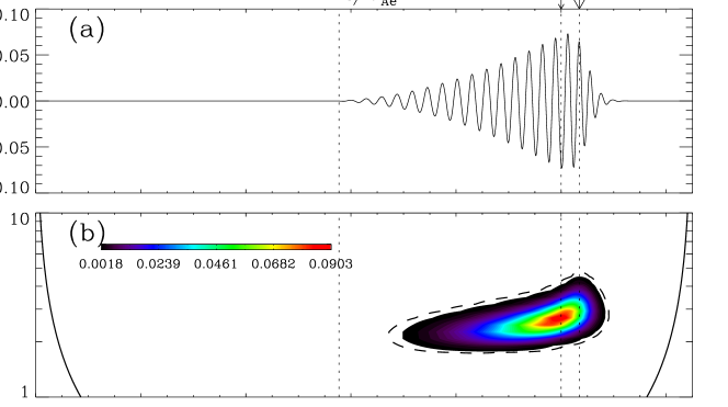
How about the “” type? To show this, let us examine a linear transition layer profile with and . The corresponding group speed diagram (the red curve in Figure 7) indicates that the M portion starts where the group speed equals . From the temporal evolution and Morelet spectrum as presented in Figure 15, one sees that indeed characterizes the onset of the most significant power. We note that higher-order sausage modes are likely to have been excited for the interval , but they cannot account for the increase in the most significant part of the Morlet power. The reason is, the critical wavenumber for the second branch is , resulting in an angular frequency of . However, the majority of the Morlet power corresponds to some , meaning that the increase in Morelet power derives from the superposition of wavepackets with along the group speed curve for the lowest-order mode. Now move on to the vertical line representing . One sees that it marks the start of the decay phase, and consequently the Morelet power starts to decrease at this point.
4 SUMMARY
Quasi-periodic propagating disturbances have been seen in a substantially number of coronal structures. While intuitively speaking this quasi-periodicity has to do with quasi-periodicities in the wave sources, it is equally possible to be caused by an impulsive driver. In this latter scenario, the frequency dependence of the longitudinal group speed is crucial for determining the temporal and spectral signatures of impulsively generated disturbances. On the other hand, while top-hat transverse density profiles have been extensively examined, little is known on how other density distributions may impact the group speed diagrams. To address this issue, we focused on sausage modes throughout, and started with an analytical study on the fully parabolic profile to show that the group speed diagrams are qualitatively the same as in the case of top-hat profiles. Both show the classical “” dependence on angular frequency . We then contrasted two more general profiles, labeled “parabolic” and “linear”, by capitalizing on our previous theoretical study on sausage waves in coronal tubes with transverse density profiles that comprise a uniform cord, a uniform external medium, and a transition layer (TL) connecting the two. Here two parameters are relevant, one being the density contrast between coronal tubes and their surroundings, and the other being the dimensionless TL width where is the mean tube radius.
For parabolic profiles, the group speed shows the typical “” behavior regardless of and . However, for linear profiles, shows a much richer variety of dependence. For low density contrasts with , the curves experience a transition from the “” to the “” type when exceeds some critical value. On the other hand, for higher density contrasts, the “” and “” types arise, meaning that the curves can posses a local maximum in addition to a minimum . With time-dependent computations, we further showed that the different behavior of group speed curves, the characteristic speeds and in particular, is indeed reflected in the temporal evolution and Morlet spectra of impulsively generated wave trains.
Given that the density structuring transverse to coronal loops remains largely unknown, it is reasonable to ask how representative the presented group speed diagrams are. In the present study, we detailed the linear profiles and showed that the dependence other than the “” behavior takes place in a rather extensive range. In fact, we have also experimented with the profiles labeled “inverse parabolic” and “sine” in our Paper I (illustrated in Figure 1b), and found that the results are qualitatively similar to the “linear” and “parabolic” cases, respectively. While it is admittedly impossible to exhaust the possible prescriptions for the transverse density distribution, our computations suggest that the group speed curves can indeed behave in a manner different from the classical “” type. On top of that, these characteristics can be discerned in the corresponding temporal and spectral evolution of impulsively generated wave trains. Observationally, this means that these wave trains can be employed not only to probe such parameters as density contrasts and density profile steepness, but also to tell the form that best describes the transverse density distribution.
References
- Asai et al. (2001) Asai, A., Shimojo, M., Isobe, H., Morimoto, T., Yokoyama, T., Shibasaki, K., & Nakajima, H. 2001, ApJ, 562, L103
- Aschwanden et al. (1999) Aschwanden, M. J., Fletcher, L., Schrijver, C. J., & Alexander, D. 1999, ApJ, 520, 880
- Aschwanden et al. (2004) Aschwanden, M. J., Nakariakov, V. M., & Melnikov, V. F. 2004, ApJ, 600, 458
- Banerjee et al. (2007) Banerjee, D., Erdélyi, R., Oliver, R., & O’Shea, E. 2007, Sol. Phys., 246, 3
- Berghmans et al. (1996) Berghmans, D., de Bruyne, P., & Goossens, M. 1996, ApJ, 472, 398
- Cally (1986) Cally, P. S. 1986, Sol. Phys., 103, 277
- Chen et al. (2015) Chen, S.-X., Li, B., Xiong, M., Yu, H., & Guo, M.-Z. 2015, ApJ, 812, 22
- De Moortel & Nakariakov (2012) De Moortel, I. & Nakariakov, V. M. 2012, Philosophical Transactions of the Royal Society of London Series A, 370, 3193
- De Pontieu et al. (2014) De Pontieu, B., Title, A. M., Lemen, J. R., Kushner, G. D., Akin, D. J., Allard, B., Berger, T., Boerner, P., Cheung, M., Chou, C., Drake, J. F., Duncan, D. W., Freeland, S., Heyman, G. F., Hoffman, C., Hurlburt, N. E., Lindgren, R. W., Mathur, D., Rehse, R., Sabolish, D., Seguin, R., Schrijver, C. J., Tarbell, T. D., Wülser, J.-P., Wolfson, C. J., Yanari, C., Mudge, J., Nguyen-Phuc, N., Timmons, R., van Bezooijen, R., Weingrod, I., Brookner, R., Butcher, G., Dougherty, B., Eder, J., Knagenhjelm, V., Larsen, S., Mansir, D., Phan, L., Boyle, P., Cheimets, P. N., DeLuca, E. E., Golub, L., Gates, R., Hertz, E., McKillop, S., Park, S., Perry, T., Podgorski, W. A., Reeves, K., Saar, S., Testa, P., Tian, H., Weber, M., Dunn, C., Eccles, S., Jaeggli, S. A., Kankelborg, C. C., Mashburn, K., Pust, N., Springer, L., Carvalho, R., Kleint, L., Marmie, J., Mazmanian, E., Pereira, T. M. D., Sawyer, S., Strong, J., Worden, S. P., Carlsson, M., Hansteen, V. H., Leenaarts, J., Wiesmann, M., Aloise, J., Chu, K.-C., Bush, R. I., Scherrer, P. H., Brekke, P., Martinez-Sykora, J., Lites, B. W., McIntosh, S. W., Uitenbroek, H., Okamoto, T. J., Gummin, M. A., Auker, G., Jerram, P., Pool, P., & Waltham, N. 2014, Sol. Phys., 289, 2733
- Edwin & Roberts (1983) Edwin, P. M. & Roberts, B. 1983, Sol. Phys., 88, 179
- Edwin & Roberts (1986) Edwin, P. M. & Roberts, B. 1986, in NASA Conference Publication, Vol. 2449, NASA Conference Publication, ed. B. R. Dennis, L. E. Orwig, & A. L. Kiplinger
- Edwin & Roberts (1988) —. 1988, A&A, 192, 343
- Frost (1969) Frost, K. J. 1969, ApJ, 158, L159
- Guo et al. (2016) Guo, M.-Z., Chen, S.-X., Li, B., Xia, L.-D., & Yu, H. 2016, Sol. Phys., 291, 877
- Jelinek & Karlicky (2010) Jelinek, P. & Karlicky, M. 2010, IEEE Transactions on Plasma Science, 38, 2243
- Jiao et al. (2015) Jiao, F., Xia, L., Li, B., Huang, Z., Li, X., Chandrashekhar, K., Mou, C., & Fu, H. 2015, ApJ, 809, L17
- Karlický et al. (2013) Karlický, M., Mészárosová, H., & Jelínek, P. 2013, A&A, 550, A1
- Katsiyannis et al. (2003) Katsiyannis, A. C., Williams, D. R., McAteer, R. T. J., Gallagher, P. T., Keenan, F. P., & Murtagh, F. 2003, A&A, 406, 709
- Kupriyanova et al. (2013) Kupriyanova, E. G., Melnikov, V. F., & Shibasaki, K. 2013, Sol. Phys., 284, 559
- Labrosse et al. (2010) Labrosse, N., Heinzel, P., Vial, J.-C., Kucera, T., Parenti, S., Gunár, S., Schmieder, B., & Kilper, G. 2010, Space Sci. Rev., 151, 243
- Lemen et al. (2012) Lemen, J. R., Title, A. M., Akin, D. J., Boerner, P. F., Chou, C., Drake, J. F., Duncan, D. W., Edwards, C. G., Friedlaender, F. M., Heyman, G. F., Hurlburt, N. E., Katz, N. L., Kushner, G. D., Levay, M., Lindgren, R. W., Mathur, D. P., McFeaters, E. L., Mitchell, S., Rehse, R. A., Schrijver, C. J., Springer, L. A., Stern, R. A., Tarbell, T. D., Wuelser, J.-P., Wolfson, C. J., Yanari, C., Bookbinder, J. A., Cheimets, P. N., Caldwell, D., Deluca, E. E., Gates, R., Golub, L., Park, S., Podgorski, W. A., Bush, R. I., Scherrer, P. H., Gummin, M. A., Smith, P., Auker, G., Jerram, P., Pool, P., Soufli, R., Windt, D. L., Beardsley, S., Clapp, M., Lang, J., & Waltham, N. 2012, Sol. Phys., 275, 17
- Li et al. (2014) Li, B., Chen, S.-X., Xia, L.-D., & Yu, H. 2014, A&A, 568, A31
- Liu & Ofman (2014) Liu, W. & Ofman, L. 2014, Sol. Phys., 289, 3233
- Liu et al. (2012) Liu, W., Ofman, L., Nitta, N. V., Aschwanden, M. J., Schrijver, C. J., Title, A. M., & Tarbell, T. D. 2012, ApJ, 753, 52
- Liu et al. (2011) Liu, W., Title, A. M., Zhao, J., Ofman, L., Schrijver, C. J., Aschwanden, M. J., De Pontieu, B., & Tarbell, T. D. 2011, ApJ, 736, L13
- Lopin & Nagorny (2014) Lopin, I. & Nagorny, I. 2014, A&A, 572, A60
- Lopin & Nagorny (2015) —. 2015, ApJ, 810, 87
- McLean & Sheridan (1973) McLean, D. J. & Sheridan, K. V. 1973, Sol. Phys., 32, 485
- Meerson et al. (1978) Meerson, B. I., Sasorov, P. V., & Stepanov, A. V. 1978, Sol. Phys., 58, 165
- Melnikov et al. (2005) Melnikov, V. F., Reznikova, V. E., Shibasaki, K., & Nakariakov, V. M. 2005, A&A, 439, 727
- Murawski & Roberts (1993) Murawski, K. & Roberts, B. 1993, Sol. Phys., 144, 101
- Murawski & Roberts (1994) —. 1994, Sol. Phys., 151, 305
- Nakariakov et al. (2004) Nakariakov, V. M., Arber, T. D., Ault, C. E., Katsiyannis, A. C., Williams, D. R., & Keenan, F. P. 2004, MNRAS, 349, 705
- Nakariakov et al. (2003) Nakariakov, V. M., Melnikov, V. F., & Reznikova, V. E. 2003, A&A, 412, L7
- Nakariakov et al. (2016) Nakariakov, V. M., Pilipenko, V., Heilig, B., Jelínek, P., Karlický, M., Klimushkin, D. Y., Kolotkov, D. Y., Lee, D.-H., Nisticò, G., Van Doorsselaere, T., Verth, G., & Zimovets, I. V. 2016, Space Sci. Rev., 200, 75
- Nakariakov & Roberts (1995) Nakariakov, V. M. & Roberts, B. 1995, Sol. Phys., 159, 399
- Nakariakov & Verwichte (2005) Nakariakov, V. M. & Verwichte, E. 2005, Living Reviews in Solar Physics, 2
- Nisticò et al. (2014) Nisticò, G., Pascoe, D. J., & Nakariakov, V. M. 2014, A&A, 569, A12
- Oliver et al. (2015) Oliver, R., Ruderman, M. S., & Terradas, J. 2015, ApJ, 806, 56
- Parks & Winckler (1969) Parks, G. K. & Winckler, J. R. 1969, ApJ, 155, L117
- Pascoe et al. (2013) Pascoe, D. J., Nakariakov, V. M., & Kupriyanova, E. G. 2013, A&A, 560, A97
- Patsourakos & Vial (2002) Patsourakos, S. & Vial, J.-C. 2002, Sol. Phys., 208, 253
- Pneuman (1965) Pneuman, G. W. 1965, Physics of Fluids, 8, 507
- Roberts (2008) Roberts, B. 2008, in IAU Symposium, Vol. 247, Waves & Oscillations in the Solar Atmosphere: Heating and Magneto-Seismology, ed. R. Erdélyi & C. A. Mendoza-Briceno, 3–19
- Roberts et al. (1983) Roberts, B., Edwin, P. M., & Benz, A. O. 1983, Nature, 305, 688
- Roberts et al. (1984) —. 1984, ApJ, 279, 857
- Rosenberg (1970) Rosenberg, H. 1970, A&A, 9, 159
- Ruderman & Roberts (2002) Ruderman, M. S. & Roberts, B. 2002, ApJ, 577, 475
- Samanta et al. (2015) Samanta, T., Pant, V., & Banerjee, D. 2015, ApJ, 815, L16
- Samanta et al. (2016) Samanta, T., Singh, J., Sindhuja, G., & Banerjee, D. 2016, Sol. Phys., 291, 155
- Selwa et al. (2007) Selwa, M., Murawski, K., Solanki, S. K., & Wang, T. J. 2007, A&A, 462, 1127
- Shen et al. (2013) Shen, Y.-D., Liu, Y., Su, J.-T., Li, H., Zhang, X.-F., Tian, Z.-J., Zhao, R.-J., & Elmhamdi, A. 2013, Sol. Phys., 288, 585
- Shestov et al. (2015) Shestov, S., Nakariakov, V. M., & Kuzin, S. 2015, ApJ, 814, 135
- Soler et al. (2014) Soler, R., Goossens, M., Terradas, J., & Oliver, R. 2014, ApJ, 781, 111
- Spruit (1982) Spruit, H. C. 1982, Sol. Phys., 75, 3
- Su et al. (2012) Su, J. T., Shen, Y. D., Liu, Y., Liu, Y., & Mao, X. J. 2012, ApJ, 755, 113
- Tian et al. (2016) Tian, H., Young, P. R., Reeves, K. K., Wang, T., Antolin, P., Chen, B., & He, J. 2016, ApJ, 823, L16
- Torrence & Compo (1998) Torrence, C. & Compo, G. P. 1998, Bulletin of the American Meteorological Society, 79, 61
- Van Doorsselaere et al. (2004) Van Doorsselaere, T., Andries, J., Poedts, S., & Goossens, M. 2004, ApJ, 606, 1223
- Wang (2016) Wang, T. J. 2016, Washington DC American Geophysical Union Geophysical Monograph Series, 216, 395
- Williams et al. (2002) Williams, D. R., Mathioudakis, M., Gallagher, P. T., Phillips, K. J. H., McAteer, R. T. J., Keenan, F. P., Rudawy, P., & Katsiyannis, A. C. 2002, MNRAS, 336, 747
- Williams et al. (2001) Williams, D. R., Phillips, K. J. H., Rudawy, P., Mathioudakis, M., Gallagher, P. T., O’Shea, E., Keenan, F. P., Read, P., & Rompolt, B. 2001, MNRAS, 326, 428
- Yang et al. (2015) Yang, L., Zhang, L., He, J., Peter, H., Tu, C., Wang, L., Zhang, S., & Feng, X. 2015, ApJ, 800, 111
- Yu et al. (2016a) Yu, H., Chen, S.-X., Li, B., & Xia, L.-D. 2016a, Research in Astronomy and Astrophysics, 16, 007
- Yu et al. (2016b) Yu, S., Nakariakov, V. M., & Yan, Y. 2016b, ApJ, 826, 78
- Yuan et al. (2013) Yuan, D., Shen, Y., Liu, Y., Nakariakov, V. M., Tan, B., & Huang, J. 2013, A&A, 554, A144
- Yuan et al. (2016) Yuan, D., Su, J., Jiao, F., & Walsh, R. W. 2016, ApJS, 224, 30