The Width Distribution of Loops and Strands in the Solar Corona – Are we Hitting Rock Bottom ?

Abstract

In this study we analyze Atmospheric Imaging Assembly (AIA) and Hi-C images in order to investigate absolute limits for the finest loop strands. We develop a model of the occurrence-size distribution function of coronal loop widths, characterized by the lower limit of widths $w_{min}$, the peak (or most frequent) width $w_{p}$, the peak occurrence number $n_{p}$, and a power law slope $a$. Our data analysis includes automated tracing of curvi-linear features with the OCCULT-2 code, automated sampling of the cross-sectional widths of coronal loops, and fitting of the theoretical size distribution to the observed distribution. With Monte-Carlo simulations and variable pixel sizes $\Delta x$ we derive a first diagnostic criterion to discriminate whether the loop widths are unresolved $(w_{p}/\Delta x\approx 2.5\pm 0.2)$, or fully resolved (if $w_{p}/\Delta x\lower 1.72218pt\hbox{$\;\buildrel>\over{\scriptstyle\sim}\;$}2.7$). For images with resolved loop widths we can apply a second diagnostic criterion that predicts the lower limit of loop widths as a function of the spatial resolution. We find that the loop widths are marginally resolved in AIA images, but are fully resolved in Hi-C images, where our model predicts a most frequent (peak) value at $w_{p}\approx$ 550 km, in agreement with recent results of Brooks et al. This result agrees with the statistics of photospheric granulation sizes and thus supports coronal heating mechanisms operating on the macroscopic scale of photospheric magneto-convection, rather than nanoflare braiding models on unresolved microscopic scales.

1 INTRODUCTION

The solar corona is permeated by invisible magnetic field lines, which can be illuminated by filling with hot coronal plasma, also called “coronal loops” or “strands”. They are supposedly field-aligned in regions with a low plasma-$\beta$ parameter. The geometry of such coronal loops can be characterized by the curvi-linear 3-D coordinates $[x(s),y(s),z(s)]$ of a potential or non-potential magnetic field line (as a function of the loop length coordinate $s$) along the loop axis, and by the cross-sectional width variation $w(s)$ in transverse direction to the loop axis. Both properties are controlled by the magnetic field. Since cross-field transport is inhibited in a low plasma-$\beta$ corona, plasma can only move along field lines, and thus the spatial organization of the coronal heating mechanism is to some extent preserved in the cross-sectional geometry and topology of loop cross-sections. In particular, we are interested in the size of the thinnest loop strands, which have been postulated in so-called “nanoflare heating” scenarios and may be detected now with the most recent instruments with the highest spatial resolution. Thus we are interested in the spatial organization and statistical distributions of loop cross sections, which may provide us clues about the geometry of the elusive coronal heating mechanism.

Previous studies on the width of coronal loop cross-sections have been focused on the finest widths that could be spatially resolved with a particular telescope (i.e., Bray and Loughhead 1985; Loughhead et al. 1985; Aschwanden and Nightingale 2005; Winebarger et al. 2013; Peter et al. 2013), unresolved strands as substructures of loops (Patsourakos and Klimchuk 2007; Aschwanden and Boerner 2011; Schmelz et al. 2013), spatial variations of loop widths $w(s)$ along loops (Wang and Sakurai 1998; Klimchuk 2000; Watko and Klimchuk 2000; Lopez-Fuentes and Klimchuk 2010), temporal loop width variations (Aschwanden and Schrijver 2011), magnetic modeling of loop width variations (Petrie 2006; Schrijver 2007; Bellan 2003; Peter and Bingert 2012), or cross-field transport of energy (Winglee et al. 1988; Amendt and Benford 1989; Chae 2002; Ruderman 2003; Georgoulis and LaBonte 2004; Vasquez and Hollweg 2004; Voitenko and Goossens 2004, 2005; Galloway et al. 2006; Ruderman et al. 2008; Erdelyi and Morton 2009; Pascoe et al. 2009; Kontar et al. 2011; Bian et al. 2011; Morton and Ruderman 2011; Arregui and Asensio-Ramos 2014; Arregui et al. 2015; Kaneko et al. 2015; Ruderman 2015). Summaries on the width of coronal loops are given in the textbooks of Bray et al. (1991; Chapters 2 and 3) or Aschwanden (2004; Chapter 5.4.4).

While theoretical models require the knowledge of the relevant coronal heating mechanisms, which are still elusive at this time, there exists essentially no theoretical prediction of the statistical distribution of loop widths in the solar corona that could be tested with current high-resolution data. However, it has been demonstrated in recent work that the statistical distributions of physical parameters in nonlinear energy dissipation processes can be modeled in terms of self-organized criticality (SOC) models (Bak, Tang, and Wiesenfeld 1987), in geology (e.g., sand piles or earthquakes), as well as in a large number of astrophysical phenomena (e.g., solar and stellar flares, pulsar glitches, soft X-ray gamma repeaters, blazars, etc., for a recent review see Aschwanden et al. 2016). In essence, SOC is a critical state of a nonlinear energy dissipation system that is slowly and continuously driven towards a critical value of a system-wide instability threshold, producing scale-free, fractal-diffusive, and intermittent avalanches with powerlaw-like size distributions (Aschwanden 2014). If we consider coronal heating events on the most basic level, in the sense of an elementary energy dissipation episode in a single loop structure, it is not much different in a solar flare or in a nanoflare (for scale-free or self-similar processes), and may be produced by the same physical mechanisms (of magnetic reconnection, plamsa heating, and cooling by thermal conduction and radiative loss), except that flares have a higher degree of spatial complexity (with multiple loops and strands) than nanoflares (within a single strand). The power law behavior in the temporal and spatial distributions of the Ohmic heating simulated in a 3D MHD model has been interpreted in terms of a SOC system specifically for the case of coronal heating (Bingert and Peter 2013). Almost every (nonlinear) instability produces ”avalanching events” over some scale-free range, in contrast to the statistics of linear random events that usually form a Gaussian probability distribution with a preferred typical (spatial) scale. Therefore, the measurement of the statistical distribution of loop widths should tell us at least whether the underlying coronal heating mechanism is a linear random process (leading to a Gaussian distribution) or a nonlinear dissipative process (leading to a power law distribution).

A size distribution exhibits a power law function over a restricted range $[x_{1},x_{2}]$ only (called the “inertial range” or “scale-free range”), and is bound by a lower limit $x_{1}$ for the smallest observed size, and by an upper limit $x_{2}$ for the largest and rarest observed size, often close to the system size. The lower limit is affected by the sensitivity threshold of the observations and the instrumental spatial resolution. The finite spatial resolution modifies the measured width also, in a predictable manner, as it can be modeled with the point spread function of the imaging instrument. These effects have never been modeled for loop width measurements, which is now possible in large statistical samples, thanks to powerful new tools of automated loop recognition software that has been developed recently (Aschwanden, De Pontieu, and Katrukha 2013a).

We will use recent high-resolution data from the Atmospheric Imaging Assembly (AIA) instrument (Lemen et al. 2012) onboard the Solar Dynamics Observatory (SDO) (Pesnell et al. 2011), and Hi-C data (Kobayashi et al. 2014) to test theoretical predictions of loop width distributions. In Section 2 we start with an analytical description of statistical width distributions. In Section 3 we describe the applied data analysis method, which includes automated pattern recognition and Principal Component Analysis (CPA) techniques. In Section 4 we conduct Monte-Carlo simulations of our automated loop width detection algorithm, in Section 5 we apply this algorithm to high-resolution AIA/SDO and Hi-C images, in Section 6 we discuss the results in the light of previous loop width measurements, and in Section 7 we present the conclusions.

2 ANALYTICAL TREATMENT

The physical parameter of interest here is the “loop width”, which we will define in terms of the equivalent width of the radial loop cross-sectional flux profile $F(r)$ in Section 3.2 (Eq. 14), being equivalent to the full width at half maximum (FWHM). In order to model size distributions of loop widths in a realistic manner we have to include threshold effects due to the finite sensitivity and spatial resolution of the instruments, which are characterized in terms of a point spread function.

2.1 The Scale-Free Probability Conjecture

As mentioned in the introduction, the statistics of nonlinear energy dissipation events often exhibit a power law-like function in their size distribution. A most general testable prediction that can be made for scale-free nonlinear energy dissipation processes is the so-called scale-free probability conjecture (Aschwanden 2012), which universally applies to self-organized criticality (SOC) systems (Bak et al. 1987), and predicts a power law distribution $N(L)$ for length scales $L$,

$$N(L)\ dL\propto L^{-D}\ dL\ ,$$ (1)

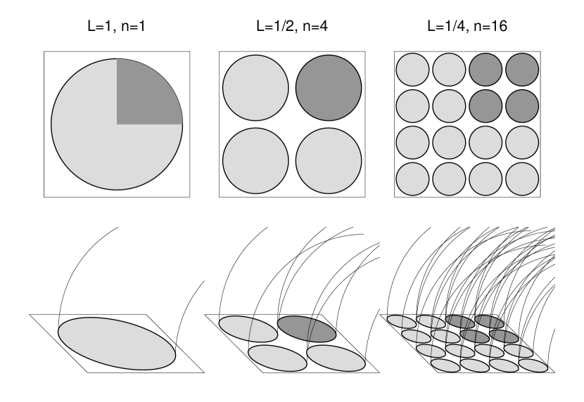
Figure 1: 2-D view (top panels) and 3-D view of an array of loop cross-sections that illustrate the reciprocal relationship between the loop width $w$ and the number $n(w)$ of loops that can be packed into a given area with a size of $L=1$. For the half size $L=1/2$ (middle panels), a total of $n=4$ loops can be fitted in. For the quarter size $L=1/4$ (right panels), a total of $n=16$ loops can be fitted in. Even when the active area of loop heating (dark grey areas) has a smaller fraction than unity ($q=0.25$ here), the relative probability of active loops with a given width $w$ is invariant.

where $D$ is the Euclidean dimension of the system. If we use the widths $w$ of coronal loops as the length scale of the cross-sectional area over which an “avalanching” mechanism dissipates energy and heats a particular coronal loop, the Euclidean dimension of cross-sectional areas is $D=2$, and thus a power law distribution of $N(w)\propto w^{-2}$ is expected. The diagram shown in Fig. 1 depicts 3 sets of loops (with widths of $w$=1, 1/2 and 1/4), which are packed into 2-D areas with identical sizes ($L=1$), yielding bundles of $n$=1, 4, and 16 strands, as expected from the size distribution specified in Eq. (1). Even when a fraction of the packing area is used only (e.g., $q=0.25$ as illustrated with dark-grey loop areas in Fig. 1), the relative probability or size distribution follows the same statistical power law relationship as specified in Eq. (1).

2.2 Thresholded Power Law Distributions

The scale-free range of a size distribution (for instance of widths $x$) exhibits an ideal power law function for the differential occurrence frequency distribution, which is characterized with a power law slope $a$,

$$N(x)\ dx\propto x^{-a}\ dx\ .$$ (2)

However, there are at least four natural effects that produce a deviation from an ideal power law size distribution, which includes: (1) A physical threshold of an instability; (2) incomplete sampling of the smallest events below a theshold; (3) contamination by an event-unrelated background; and (4) truncation effects at the largest events due to a finite system size, which all can be modeled with a so-called “thresholded power law” distribution function, also called Pareto [type II] or Lomax distribution (Lomax 1954),

$$N(x)\ dx\propto(x+x_{0})^{-a}\ dx\ ,$$ (3)

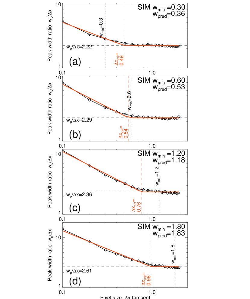
Figure 8: The peak widths (normalized by the pixel size) $w_{p}/\Delta x$, are shown as a function of the pixel size $\Delta x$, measured from 20 simulated size distributions with pixel sizes of $\Delta x=0.1\hbox{${}^{\prime\prime}$},...,2.0\hbox{${}^{\prime\prime}$}$, for four sets of numerical simulations, with $w_{min}=0.3\hbox{${}^{\prime\prime}$}$ pixel (a), $w_{min}=0.6\hbox{${}^{\prime\prime}$}$ pixel (b), $w_{min}=1.2\hbox{${}^{\prime\prime}$}$ pixels (c), and $w_{min}=1.8\hbox{${}^{\prime\prime}$}$ pixels (d). The simulated values are indicated with diamonds, and best-fit models are overlaid with red solid curves. The simulated minimum loop widths $w_{min}$ are indicated with black vertical lines, while the predicted values $w_{pred}$ are shown with red (dashed) vertical lines, predicted by the critical value $w_{p}/\Delta x=3.0$ (horizontal black dashed line).

which was found to fit flux distributions of solar and stellar flare data well, in the scale-free range $x\lower 1.72218pt\hbox{$\;\buildrel>\over{\scriptstyle\sim}\;$}x_{0}$ (Aschwanden 2015). The additive constant $x_{0}$ turns a power law function into a constant for small values $x\ll x_{0}$ at the left side of a size distribution (Fig. 2a; dashed curve), a feature that fits some data, but not all. Examples for different phenomena are shown in Fig. 8 of Aschwanden (2015), based on data presented in Clauset et al. (2009). The functional shapes of size distributions are shown in Fig. 2, which shows the ideal power law slope at $x\gg x_{0}$ (Eq. 2; thin solid line in Fig. 2a), and the thresholded power law function (Eq. 3; dashed line in Fig. 2a), where the threshold is set at $x_{0}/w_{min}=2.5$, all shown on a log-log scale in Fig. 2.

2.3 Minimum Loop Widths

Since we are going to analyze the contributions of the thinnest loop strands to the size distribution of loop widths, we have to include a number of effects that set a lower limit on the measurement of loop widths, such as the finite instrumental spatial resolution and loop background noise, which we discuss in more detail with a quantitative example in Section 2.5. At this point we combine these effects into the variable $w_{min}$, which represents an absolute lower limit in the theoretical model distribution of loop widths $w$. The effectively detected loop width (or observed loop width) $w$ can be defined in terms of adding the true loop width $w_{true}$ and the combined broadening effects expressed in $w_{min}$ in quadrature,

$$w=\sqrt{w_{true}^{2}+w_{min}^{2}}\ ,$$ (4)

so that the true width $w_{true}$ can be obtained from the observables $w$ and $w_{min}$,

$$w_{true}=\sqrt{w^{2}-w_{min}^{2}}\ .$$ (5)

Substituting the variable $x(w)$ into the thresholded distribution function $N(w)dw=N(x[w])$ $|dx/dw|\ dw$ (Eq. 3), where we denote $x=w_{true}$ (in Eq. 5) and $w_{min}=x_{0}$ (in Eq. (3)), and inserting its derivative, $dx/dw=w/\sqrt{w^{2}-w_{min}^{2}}$, we obtain then the theoretical size distribution $N(w)$ of apparent (or modeled observed) loop widths $w$,

$$N(w)\ dw\propto\left\{\begin{array}[]{ll}0&{\rm for}\ w\leq w_{min}\\ w\ \left(w^{2}-w_{min}^{2}\right)^{-1/2}\left(\sqrt{(w^{2}-w_{min}^{2})}+w_{min}\right)^{-a}\ dw&{\rm for}\ w>w_{min}\end{array}\right.\ .$$ (6)

which is shown in Fig. 2a (dash-dotted line) as a function of the normalized width $w/w_{min}$. Thus, the spatial resolution causes an upturn with an excess above the thresholded power law distribution right near $w/w_{min}\lower 1.72218pt\hbox{$\;\buildrel>\over{\scriptstyle\sim}\;$}1$, while no events are detected below the limit $w/w_{min}=1$. However, the sharp peak at $w/w_{min}=1$ may not be observable, because the loop width measurements have inherently some uncertainties that smooth out such sharp peaks in the observed size distributions, and show the most frequent detections at a peak value of $w_{p}/w_{min}\approx 2.5$, rather than at the absolute limit $w/w_{min}=1$ (see numerical simulations in Section 4 and point-spread functions of EUV imaging instruments, compiled in Table 3 and references therein).

2.4 Power Law with a Smooth Cutoff

In our data analysis, the width $w$ of a loop cross-section is measured from the equivalent width of a Gaussian-like loop flux profile, where a local background is subtracted with a lowpass filter, and the high-frequency data noise is filtered out with a highpass filter. This method, as well as many others, produce uncertainties in the loop width measurement of order of one pixel for the thinnest loop strands, mainly because the true background flux profile is unknown and perturbed by data noise. As a consequence, the size distribution of loop widths exhibits a smooth drop-off towards the minimum value at $w\lower 1.72218pt\hbox{$\;\buildrel>\over{\scriptstyle\sim}\;$}w_{min}$.

In order to provide a realistic analytical model of a size distribution that can reproduce such an absolute cutoff value we have to replace the threshold parameter $w_{\mathrm{min}}$ with a reciprocal function $1/(w-w_{min})$ that has a singularity at $w=w_{\mathrm{min}}$,

$$N(w)\ dw=n_{0}\left({w+{w_{0}^{2}\over(w-w_{min})}}\right)^{-a}\ dw\ ,$$ (7)

where we introduced an arbitrary constant $w_{0}$, to be determined. This type of distribution contains the desired singularity at $w=w_{min}$, and setting it to zero for smaller values $w<w_{min}$ enforces an absolute lower cutoff at $w=w_{min}$.

We explore the maximum of this distribution function by setting the derivative to zero, i.e., $dN/dw|_{w=w_{p}}=0$, and find that the peak value $w_{p}$ of the distribution function (Eq. 7) is related to the constant $w_{0}$ by,

$$w_{0}=(w_{p}-w_{min})\ ,$$ (8)

while the maximum value $N_{p}$ of the distribution function at $w_{p}$ amounts to,

$$N_{p}=N(w=w_{p})=n_{0}(2w_{p}-w_{min})^{-a}\ .$$ (9)

Inserting the constant $w_{0}$ (Eq. 8) into the distribution function $N(w)$ (Eq. 7) yields then,

$$N(w)\ dw=\left\{\begin{array}[]{ll}0&{\rm for}\ w\leq w_{min}\\ n_{0}\left({w+{(w_{p}-w_{min})^{2}\over(w-w_{min})}}\right)^{-a}\ dw&{\rm for}\ w>w_{min}\end{array}\right.\ .$$ (10)

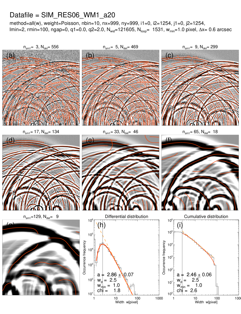
Figure 6: Seven bipass-filtered images (grey scale) with filters of $n_{sm1}=2,4,8,16,32,64,128$ pixels, produced from the original image shown in Fig. 5a. The automated loop detection is visualized with red curves in each of the 7 filters. The differential and cumulative size distributions of the histogrammed loop widths (histograms with error bars) are fitted with the theoretical distribution function consisting of a power law with a smooth cutoff (Fig. 2b), defined in Eq. (11) (red curves). The power law slope is indicated with a dashed orange line.

This definition of a size distribution has the following properties, which are illustrated in Fig. 2: (1) The distribution has two regimes, a scale-free range at large values $(w_{p}<w<w_{max})$ that follows a power law function, and a smooth cutoff range at small values $(w_{min}<w<w_{p})$; (2) A peak of the distribution $N_{p}=n(w=w_{p})$ at the value $w=w_{p}$; (3) The size distribution is completely defined in the entire range of $(w_{min}<w<w_{max})$ with an absolute lower cutoff at $w\approx w_{min}$; (4) The distribution function can be represented with four parameters ($n_{0},w_{0},w_{min},a)$, or more conveniently expressed in terms of the peak parameters, $(N_{p},w_{p},w_{min},a)$, with $N_{p}=n_{0}(2w_{p}-w_{min})^{-a}$ and $w_{p}=w_{min}+w_{0}$. Since the parameter $w_{min}$ is a constant for a given instrument, only the three parameters $(n_{0},a,w_{p})$ need to be optimized in a fitting procedure for each data set. A family of such size distributions with various peak values $w_{p}$ is depicted in Fig. 2b. We will see that this type of power law distribution with a smooth cutoff range $[w_{min},w_{p}]$ suits the observed size distributions much better (Figs. 6h, 10h, 14h) than the thresholded power law function with the threshold constant $x_{0}=w_{min}$ (Eq. 3), or the sharply peaked power law function with a lower cutoff at the spatial resolution $w_{min}$ (Eq. 6).

2.5 Loop Width Broadening Effects

Let us discuss the physical meaning of the minimum loop width $w_{min}$ that we introduced in the previously defined theoretical distributions. The major contribution to the minimum detected loop width is the instrumental point-spread function $w_{psf}$. Typically, the instrumental point-spread function of EUV or soft X-ray telescopes amounts to $w_{psf}\approx 2.0-2.5$ pixels of the CCD detectors, mostly dictated by the electronic charge spreading. For instance, the azimuthally-averaged point-spread function of the Transition Region and Coronal Explorer (TRACE) has been determined with a blind iterative deconvolution technique to be $\approx$2.5 pixels, or $1.25\hbox{${}^{\prime\prime}$}$ (Golub et al. 1999).

In addition, the measured loop widths are affected by data noise in the subtracted background counts in every pixel, which is most severe for faint loops on top of a strongly varying background, especially since we apply a high-pass filtering technique (rather than a Gaussian fitting of loop cross-section profiles). From numerous tests we evaluated that this loop width broadening component has a standard deviation of $w_{noise}\approx 1$ pixel. A more detailed discussion of this quantity including Quiet-Sun background counts, Poissonian photon noise, readout noise, digitization noise, lossless compression, pedestal dark current, integer subtraction, and spike residuals is given for the TRACE instrument in Aschwanden et al. (2000c).

Combining these loop width broadening effects by summing in quadrature we specify an observed loop width $w$ by,

$$w^{2}=w_{true}^{2}+w_{psf}^{2}+w_{noise}^{2}\ ,$$ (11)

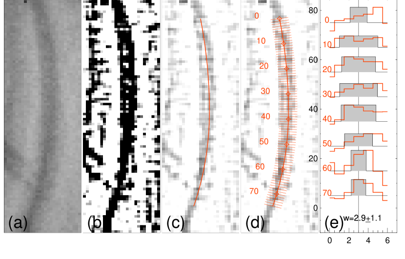
Figure 4: Example of loop width measurements along a loop segment: (a) flux of original AIA image; (b) bipass-filtered image with highpass filter of $n_{sm1}=3$ pixels and lowpass filter $n_{sm2}=5$ pixels; (c) Automated loop tracings above a noise threshold (of 2 standard deviations of background) with OCCULT-2 code; (d) Curved array along a traced loop (red curve) with a width range of $n_{w}=n_{sm1}+4=7$ pixels; (e) Interpolated cross-sectional flux profiles (red histograms) in perpendicular direction to the loop axis, with equivalent-width measurements (grey rectangles), yielding a mean width of $w=2.9\pm 1.1$ pixels.

where $w_{true}$ represents the unknown true width for a given loop segment. A quantitative example is illustrated in Fig. 4e, where a mean FWHM width of $w=2.9\pm 1.1$ pixels is measured from 75 loop cross-sections. If we estimate a point-spread function width of $w_{psf}=2.5$ pixels, a data noise component of $w_{noise}\approx 1.0$ pixel, we obtain with Eq. (11) a true loop width of $w_{true}=[w^{2}-w_{psf}^{2}-w_{noise}^{2}]^{1/2}\approx[2.9^{2}-2.5^{2}-1.0^{2}]^{1/2}\approx 1.1$ pixels. Thus, the expected minimum observed loop width for unresolved loop strands (with $w_{true}\ll 1$ pixel) is $w_{min}=[w_{psf}^{2}+w_{noise}^{2}]^{1/2}\approx 2.7$ pixels.

In summary, the following symbols are used for loop widths: $w$ is generally used for the observed (or modeled observed) loop width, $w_{true}$ is the true (fully resolved) loop width, $w_{min}$ is the minimum width in the theoretical model distribution, $w_{sim}$ is the simulated loop width, $w_{psf}$ is the point-spread function, and $w_{noise}$ is the broadening due to background subtraction data noise. In the numerical simulations, an instrumental point-spread function with a width of $w_{psf}=2.5$ pixels is applied.

3 DATA ANALYSIS METHOD

Our data analysis method consists of two major steps: (1) The automated loop detection, and (2) a Principal Component Analysis (PCA) applied to generate loop width distributions.

3.1 Automated Loop Detection

The automated detection of features with a large range of spatial scales is not trivial, especially when small and large structures coexist and blend into each other, or overlap with each other, as it is the case for a solar corona image with many different loops along any given line-of-sight.

We make use of an already existing automated loop detection code, the so-called Oriented Coronal CUrved Loop Tracing code OCCULT-2 (Aschwanden et al. 2008c, 2013a; Aschwanden 2010), which is customized for automated detection of curvi-linear coronal (or chromospheric) loops (or fibrils) with relatively large curvature radii, compared with their cross-sectional width. The numerical code, written in the Interactive Data Language (IDL) is publicly available in the SolarSoftware (SSW) library, with a tutorial given at http://www.lmsal.com/$\sim$aschwand/software/tracing/tracing$\_$tutorial1.html . The OCCULT-2 code can be applied to any 2-D image with an intensity (or flux) distribution $F(x,y)$, from which the cartesian coordinates $[x(s),y(s)]$ of a set of 2-D curvi-linear structures as a function of their length coordinate $s$ are determined. Applications range from solar EUV images of the Transition Region And Coronal Explorer (TRACE), AIA/SDO, H$\alpha$ images of the Swedish Solar Telescope (SST), to microscopic images of microtubule filaments in live cells in biophysics (Aschwanden et al. 2013a). We provide in the following a brief description of the OCCULT-2 code.

The original image is first filtered with a highpass filter (with a smoothing 2-D box car with a length of $n_{sm1}$ pixels), and with a lowpass filter (with a smoothing 2-D box car with a length of $n_{sm2}$), which together act as a highpass filter for curvi-linear structures with a (transverse) length scale range of $[n_{sm1},n_{sm2}]$, where the bipass-filtered image is defined as,

$$F_{bipass}(x,y)=smooth{[F(x,y),n_{sm1}]}-smooth{[F(x,y),n_{sm2}]}\ .$$ (12)

The highpass filtering of an image is also known as unsharp masking.

The numerical algorithm of automated curvi-linear pattern detection works as follows. First, the image location $[x_{1},y_{1}]$ of the maximum flux $F_{max}(x_{1},y_{1})=max[(F_{bipass}(x,y)]$ is detected, from where the search of the first structure (with the highest contrast) starts, by detecting the directional angle $\alpha([x_{1},y_{1}])$ of the local ridge (Fig. 3),

$$\alpha([x_{1}(s),y_{1}(s)]=\arctan{\left({dy/ds\over dx/ds}\right)}\ .$$ (13)

In addition, the curvature radius $r_{curv}(x_{0},y_{0})$ of the local ridge is determined also in order to obtain a second-order polynomial approximation of the traced loop structure. A geometric diagram of the parameterized first and second-order elements measured in a single point of a curvi-linear ridge is shown in Fig. 3. Then the same direction is extrapolated in second-order as an approximate prediction for the continuation of the loop direction. The exact direction of the traced loop segment at the next loop coordinate $s_{i+1}=s_{i}+\Delta s$ is then evaluated by maximizing the cross-correlation coefficient between the (generally gaussian-like) subsequent loop cross-sectional profile $F[r,\alpha(s_{i+1})]$ compared with the previous profile $F[r,\alpha(s_{i})]$. If the direction of the loop tangent is ${\bf s}=[dx/ds,dy/ds]$, the perpendicular direction is defined by ${\bf r}=[-dy/ds,dx/ds]$, along which the cross-sectional loop profile $F(r)$ is defined. The automated loop detection continues from $s_{i}$ to $s_{i+1}=s_{i}+\Delta x$ in the first loop segment step, and then from $s_{i+1}$ to $s_{i+2}$ in the second loop segment step, and so forth. The end of the first half loop segment occurs when the bipass-filtered flux values drop below a selectable threshold (typically set at one standard deviation of the flux of the background variation). The code traces then the second half of the loop segment in the same way, except in reverse direction, starting from the initial maximum value at $[x_{1},y_{1}]$. Once the end of the second half loop segment is reached, both the first and second half segments are joined together in the same direction, which constitutes the coordinates $[x(s_{i}),y(s_{i})],i=0,...,n_{p}$ with $n_{p}$ points of the full loop segment. The image area that covers the coordinates of the first loop, with a margin of $\pm n_{sm1}$ pixels in $x$ and $y$-direction, is then erased in the bipass-filtered image, so that an already traced loop segment is not used multiple times in the tracing of a new structure. This procedure of detecting the first loop is then continued at the location of the next image maximum $[x_{2},y_{2}]$ and repeated for the structure with the second-highest contrast, and so forth, until the zero floor or a preset threshold value in the bipass-filtered image is reached. In the end the code produces a list of $[x_{j}(s_{i}),y_{j}(s_{i})]$ loop coordinates for $j=1,...,n_{j}$ loop segments, each one containing $i=1,....,n_{i}$ coordinate points.

There are a few control parameters that can be set in the OCCULT-2 code, such as the maximum number of traced structures $n_{struc}$ per image or wavelength, the highpass filter $n_{sm1}$, the lowpass filter $n_{sm2}$, the minimum accepted loop length $l_{min}$, the minimum allowed curvature radius $r_{min}$, the field line step $\Delta s$ along the (projected) loop coordinate, the flux threshold $q_{thresh1}$ (in units of the median value of positive fluxes in the original image), the filter flux threshold $q_{thresh2}$ (in units of the median value in the positive bipass-filtered fluxes), the maximum allowed gap $n_{gap}$ with zero or negative fluxes along a traced ridge. In our analysis we choose the following default control parameters: $n_{sm1}=1,...,64$ pixels, $n_{sm2}=n_{sm1}+2$ pixels, $l_{min}=2$ pixels, $r_{min}=100$ pixels, $\Delta s=1$ pixel, $q_{thresh,1}=0$, $q_{thresh,2}$=2, and $n_{gap}=0$. We will present some parametric studies in Section 4 in order to investigate systematic trends of the algorithm.

3.2 Principal Component Analysis

The OCCULT-2 code applies a bipass-filter to an image $F(x,y)$, consisting of a highpass filter with a selectable smoothing boxcar length $n_{sm1}$, and a lowpass filter with a boxcar length $n_{sm2}$. Such a bipass filter selects only structures within the width range of $[n_{sm1},n_{sm2}]$ in the automated pattern recognition algorithm. The narrowest possible width for a bipass filter is $n_{sm2}=n_{sm1}+2$, which yields a highest sensitivity to detect structures with a width of $w\approx(n_{sm1}+n_{sm2})/2$. For instance, if we set a lowpass filter of $n_{sm1}=2$, the highpass filter is $n_{nsm2}=n_{sm1}+2=4$, and the selected loop widths are $w\approx(n_{sm1}+n_{sm2})/2=(2+4)/2=3\pm 1$. An example of an automatically traced loop with extraction of the loop width profiles in perpendicular direction to the loop axis is shown in Fig. 4. The actual loop width $w$ at a given loop location $s_{i}$ along a loop is measured from the equivalent width $w$ of the loop cross-sectional flux profile $F(r)$,

$$w={\int F(r)dr\over max[F(r)]}\ ,$$ (14)

where the coordinate $r$ is defined in perpendicular direction to the local loop axis $s$, and the value $F_{ij}=F(s_{i},r_{j})$ at a particular location $(s_{i},r_{j})$ is obtained from bilinear extrapolation in the 2-D image $F(x,y)$. In the example shown in Fig. 4e, the mean loop width is found to be $w=2.9\pm 1.1$ pixels, where the uncertainty mostly results from the point-spread function, the noisy background, and multiple overlapping loop strands. The automated measurement of loop widths is performed in steps of $\Delta s=1$ pixels along each loop segment, which typically yields 10-100 times more width measurements than loop detections.

For the detection of structures with cross-sectional widths covering a range of two decades, we can select a series of independent filter width components that are increasing by powers of two,

$$n_{sm1,k}=2^{k}\ ,\qquad k=0,1,...6\ ,$$ (15)

which essentially corresponds to the orthogonal basis functions in Fourier transforms or in Principal Component Analysis (PCA) techniques (e.g., Jackson 2003). PCA techniques have been applied to solar physics data sets in various ways (e.g., Lawrence et al. 2004; Casini et al. 2005; Cadavid et al. 2008; Zharkova et al. 2012). Hence, we can run the automated loop detection for every image multiple times with independent (orthogonal) bipass filters $n_{sm1,k}$, in order to obtain a completely sampled range of width measurements. The smallest smoothing boxcar width ($n_{sm1,0}=1$ pixel) approximately corresponds to the instrumental resolution, while an upper limit of $n_{sm1,6}=2^{6}=64$ pixels covers about two orders of magnitude in the range of width measurements, with $w_{max}=2^{6}=64$ pixels.

The choice of filters by powers of 2 yields a uniform distribution of widths $w_{i},i=0,...,6$ on a logarithmic scale, $log{(w)}$. The OCCULT-2 code yields then a number of detected loop structures $N_{i},i=0,...,6$ for each selected width $w_{i}$. This yields directly a frequency occurrence distribution (or size distribution) $N(w)$ of loop structures, which is generally displayed on a $log(N)-log(S)$ (Number versus Size) plot. In other words, the option of width filters in the OCCULT-2 code can be directly used for the measurement of size distributions $N(w)$. Of course, structures that are detected on relatively large scales of $w\gg 1$ Mm, are likely to consist of more complex structures (e.g., arcades of loops), rather than traditional field-aligned monolithic loops. The size distributions can have different functional shapes, each one being a characteristic of the underlying physical process. For instance, random measurements of linear processes yield a Gaussian normal distribution, while nonlinear dissipative processes yield a power law distribution. By measuring the size distribution, we obtain thus a diagnostic of the underlying (linear or nonlinear) physical generation mechanism.

4 MONTE-CARLO SIMULATIONS

In order to test and validate the numerical code to measure the size distributions $N(w)$ of loop widths $w$ within a specified range, we present a basic Monte-Carlo simulation (Section 4.1), and investigate the effect of finite spatial resolution on the inferred loop width size distribution $N(w)$ (Section 4.2).

4.1 Basic Monte-Carlo Simulation

We generate a thresholded power law size distribution of loop widths, with a threshold at $w_{0}$ (according to Eq. 3), where the symbol $w_{sim}$ stands here for the simulated fully resolved loop widths,

$$N(w_{sim})\ dw_{sim}\propto(w_{sim}+w_{0})^{-a}\ dw_{sim}\qquad{\rm for}\ w_{sim}\geq w_{min}\ ,$$ (16)

with a power law index of $a=2$, bound by the range $[w_{min},w_{max}]$. Such a distribution can be produced by using the transformation (e.g., Section 7.1 in Aschwanden 2011; Eq. 15 in Aschwanden 2015),

$$w_{sim,i}=\left[(1-\rho_{i})(w_{min}+w_{0})^{(1-a)}+\rho_{i}(w_{max}+w_{0})^{(1-a)}\right]^{(1/(1-a)}-w_{0}\ ,$$ (17)

where $\rho_{i}$ are random numbers uniformly distributed in the interval $[0<\rho_{i}<1]$. Such a set of values $w_{sim,i}$ forms then a size distribution $N(w_{sim})$ of widths in form of a power law function. The peak value of the cross-sectional loop profiles $F(r)$ are chosen according to the emission measure definition in an optically thin plasma,

$$F_{i}\propto\int n_{e}^{2}\ dz\propto\langle n_{e}^{2}\rangle w_{sim,i}\propto w_{sim,i}\ ,$$ (18)

where the mean electron density $\langle n_{e}\rangle$ is assumed to be independent of the loop width, which means that the flux increases proportionally to the column depth $w=\int dz$, being equal to the loop width $w_{sim,i}$ for circular loop cross-sections. Note that the simulated loop widths $w_{sim,i}$ defined in Eqs. (16-18) are fully resolved, because each simulated loop strand is made up of numerical sub-strands with a width of 1 pixel.

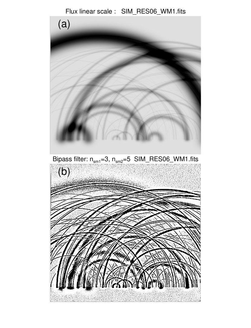
Figure 5: (a): Monte-Carlo simulation of loop image with 128 randomly distributed loops that have a power law distribution of loop widths $N(w_{sim})\propto(w_{sim}+w_{0})^{-a}$ with a power law slope $a=2.0$ and resolution $w_{0}=1$ pixel; (b): Bipass-filtered image with filters $n_{sm1}=3$ and $n_{sm2}=5$, which filters out structures with widths of $w=4\pm 1$.

A spatial 2-D image $F(x,y)$ is then composed by superposing the brightness distributions of semi-circular loops (as shown in Fig. 5), each one consisting of a space-filling bundle of loop strands with a total Gaussian cross-section of width $w_{sim,i}$ (Eq. 17) and flux $F_{i}$ (Eq. 18). The loop positions are randomly distributed in 2-D space with a fixed height of the curvature center (of the semi-circular loops) in photospheric height. In this set up we simulate a total of $n=128$ loop bundles, where the strands have a cutoff or minimal width of $w_{0}=1$ pixel, projected into a 2-D image with a size of $1000\times 1000$ pixels. In addition, the simulated images are convolved with a 2D Gaussian kernel that has a FWHM of $w_{psf}=2.5$ pixels in order to mimic a realistic instrumental point-spread function. The peak count rate is $10^{5}$ photons per pixel, and a background with random noise of 10% is added. An example of such a simulated image is shown in Fig. 5a, along with a bipass-filtered rendering in Fig. 5b. The added random noise is visible in the filtered image in Fig. 5b.

We perform now a validation test of the capability to retrieve the underlying power law distribution function of loop widths as follows. We apply seven bipass filters with $n_{sm1}=2^{i}=1,2,4,8,16,32,64$ and $n_{sm2}=n_{sm1}+2$ to produce seven bipass-filtered images with different filter widths. This corresponds to the principal component analysis (PCA) described in Section 3.2. We run the automated loop detection code OCCULT-2 on each of the 7 images, using a threshold of $q_{2}=2.0$ standard deviations (in the bipass-filtered image), we require a minimum length of $l_{min}=2$ pixels for the selected loop length segments, and show the detected loop tracings in Fig. 6 (red curves), which appear to be fairly complete in all filters, as judged by visual detection. Comparing the detected structures with the theoretically simulated image (Fig. 5a) on a pixel-by-pixel basis, we find that 80% of the simulated image pixels are retrieved with the correct values, using the automated OCCULT-2 code. Then we fit the histograms of loop widths, which includes 152,564 loop widths measurements in 1254 loop segments detected in 7 different filter images. For the power law slopes of the resulting width distributions we find the values of $a=2.82\pm 0.07$ for the differential frequency distribution (Fig. 6h), and a similar value from the cumulative frequency distribution (Fig. 6i).

The specific value of the power law slope $a$ cannot easily be retrieved with our method, since most loops show up in multiple width filters, and thus are counted multiple times with different widths. We tested input values of the power law slope in the range of $a=1.5-4.0$ in the simulations, but obtained invariably values of $a\approx 2.7\pm 0.2$ after auto-detection with our multi-scale sampling method. A method for the power law slope retrieval can in principle be designed by eliminating multiple countings of loops, but this requires a unique definition of the mathematical function of loop cross-section profiles, which is an ambiguous task and is not necessary for the measurement of the size distribution of the smallest loop strands here.

Inspecting the peak of the size distribution of widths $N(w_{sim})$, we find a peak width of $w_{p}/w_{min}=3.0$ (Figs. 6h, 6i). The reduced chi-square value of $\chi=1.9$ (Fig. 6h) is satisfactory for the fit of the differential size distribution, given the simple analytical model used here (Eq. 10).

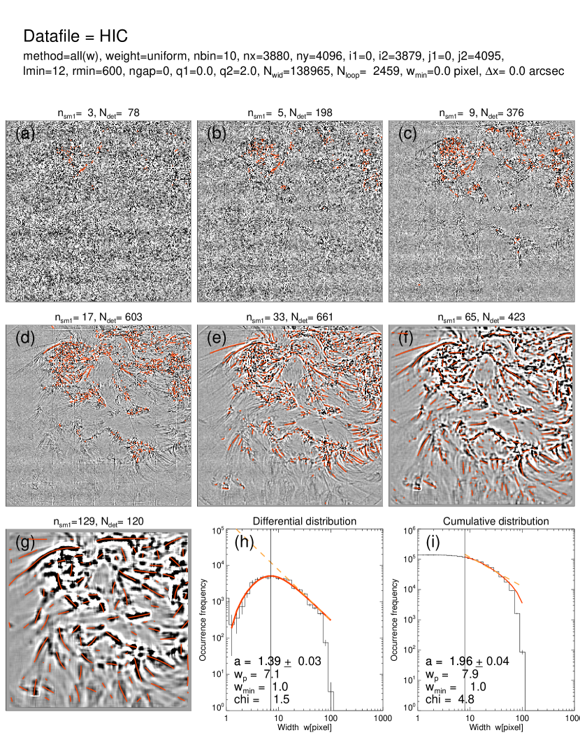
Figure 13: Seven bipass-filtered images (grey scale) with filters of $n_{sm1}=2,4,8,16,32,64,128$ pixels and automated loop tracings (red curves), obtained from the HiC image at a wavelength of 193 Å as shown in Fig. 11a. Otherwise similar representation as in Fig. 6.

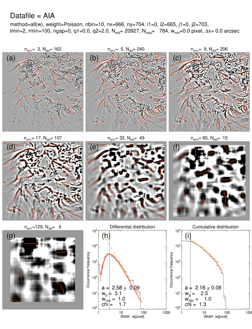
Figure 14: Seven bipass-filtered images (grey scale) with filters of $n_{sm1}=2,4,8,16,32,64,128$ pixels and automated loop tracings (red curves), obtained from the AIA/SDO image at a wavelength of 193 Å. Otherwise similar representation as in Fig. 13.

Thus this test demonstrates that we can (1) measure a complete size distribution of loop widths within a range of about two orders of magnitude above the instrumental resolution limit, (2) retrieve the functional shape of a power law function (although not the exact value of the power law slope), and (3) detect the rollover of a smooth cutoff in the range of $1\leq w_{sim}/w_{min}\lower 1.72218pt\hbox{$\;\buildrel<\over{\scriptstyle\sim}\;$}3$ pixels near the resolution limit $w_{min}$. Comparing simulated loop images (Fig. 6) with observed images (Figs. 13-14), however, we notice that the numerical simulations contain idealized loops only, without taking temperature inhomogeneities into account, such as “moss structures” at the footpoints of hot soft X-ray emitting loops (e.g., Berger et al. 1999). The present study therefore does not discriminate between “classical coronal loops” and “loop-like transition region phenomena”, nor does it disentangle the 3D topology of nested loop structures. Nevertheless, the sampling is complete in the 2D image plane (thanks to the automated loop detection algorithm), and thus no ad hoc assumptions of loop selection criteria are applied, which makes it more suitable to compare with theoretical models of statistical distributions, rather than a hand-picked sample of selected (loop) structures.

4.2 Detecting the Cutoff of the Smallest Loop Strands

The detection of a lower cutoff for the widths of the smallest loop strands depends crucially on the spatial resolution or pixel size of the image. In a Monte-Carlo simulation we can vary the spatial resolution and study the effect of the spatial resolution limit on the detection of the finest loop strands. In the basic example shown in Fig. 6 we have chosen a minimum loop strand width of $w_{min}=1$ image pixel, and sampled the size distribution in the range between $w_{min}=1$ and $w_{max}=10^{2}$ pixels (Figs. 6h and 6i). We note that the resulting differential occurrence frequency distribution shown in Fig. 6h exhibits a peak at a width ratio of $w_{p}/w_{min}\approx 3.0$. It turns out that this ratio of the peak width to the pixel size is a persistent feature in our simulations of power law distributions $N(w_{sim})$ of loop widths, for samples with unresolved structures down to the pixel size $\Delta x$.

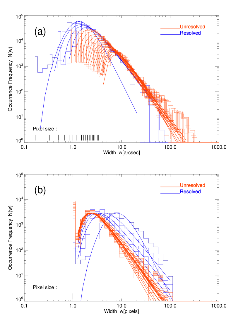
Figure 7: (a) A set of 20 size distributions from identical Monte-Carlo simulations is shown (with a minimum loop width of $w_{min}=0.6\hbox{${}^{\prime\prime}$}$, but different pixel sizes or spatial resolutions (for $\Delta x=0.1\hbox{${}^{\prime\prime}$},0.2\hbox{${}^{\prime\prime}$},...,2.0\hbox{${}^{\prime\prime}$}$). The obtained size distributions are rendered as histograms, the analytical fits of the unresolved cases ($w_{min}<\Delta x$) with red curves, and the resolved cases ($w_{min}>\Delta x$) with blue curves. (b) The fits are normalized by their pixel sizes and peak occurrence rates in diagram (b), which shows the universal shape (red curves) for the unresolved cases.

In order to investigate the universality of this ratio of the peak value $w_{p}$ of a size distribution $N(w_{sim})$ to the pixel size $\Delta x$ we perform 20 numerical simulations of identical 2-D images (the same as shown in Fig. 5a), but with 20 different pixel sizes, from $\Delta x=0.1\hbox{${}^{\prime\prime}$}$ to $\Delta x=2.0$ ^′′, while the scaling of the standard simulation shown in Fig. 6 corresponds to an AIA pixel with $\Delta x=0.6\hbox{${}^{\prime\prime}$}$. For conversion into units of Mm we use the scaling $1\hbox{${}^{\prime\prime}$}$ (arcsec)=0.725 Mm. We overlay the histograms and power law fits of the 20 size distributions with different pixel sizes in Fig. 7a, which shows a systematic shift of the peak with pixel size. However, when we normalize the size distributions $N(w_{sim})$ to the pixel size $\Delta x$ on the x-axis, and to the peak value $N_{p}=N(w_{sim}=w_{p}$) on the y-axis, we see that the peaks line up at a peak value of $w_{p}\approx 3.0\Delta x$ (Fig. 7b), and thus the normalized size distribution of loop widths exhibits a universal shape. However, this is only true for distributions that do not resolve the finest loop strands (red curves in Fig. 7), when the smallest loop width is smaller than the pixel size, while the distributions with pixel sizes smaller than the finest loop widths exhibit a larger ratio $w_{p}/\Delta x\lower 1.72218pt\hbox{$\;\buildrel>\over{\scriptstyle\sim}\;$}3.0$ of the peak width to the pixel size, because there is a relative scarcity of detected loops at small widths $w_{sim}$. Thus we can use the ratio $w_{p}/\Delta x$ as a diagnostic for discriminating which size distributions resolve, or do not resolve, the smallest loop strands.

In order to quantify this new diagnostic criterion we perform $4\times 20$ Monte-Carlo simulations, for four different cutoffs $w_{min}$ of the loop width distributions, $w_{min}=0.3\hbox{${}^{\prime\prime}$}$, $0.6\hbox{${}^{\prime\prime}$}$, $1.2\hbox{${}^{\prime\prime}$}$, and $1.8\hbox{${}^{\prime\prime}$}$, and for 20 different spatial resolutions $\Delta x=0.1\hbox{${}^{\prime\prime}$},0.2\hbox{${}^{\prime\prime}$},...,2.0\hbox{${}^{\prime\prime}$}$. For each of the 80 simulated images we repeat the automated loop detection, produce the size distributions of loop widths, and measure the ratio of the peak width to the pixel size, $w_{p}/\Delta x$. The results of these ratios as a function of the pixel size are plotted in Fig. 8 (black diamonds). From the four plots in Fig. 8 we see that each function $w_{p}/\Delta x$ exhibits two regimes, a fully resolved regime at $w<w_{min}$ on the left, and an unresolved regime at $w>w_{min}$ on the right side. We can model this dependence of the peak width $q_{w}=w_{p}/\Delta x$ on the spatial resolution $\Delta x$ with the function $q_{w}(\Delta x)$,

$$q_{w}=\sqrt{\left({w_{min}\over\Delta x}\right)^{2}+\left(w_{psf}\right)^{2}}\ ,$$ (19)

for which best fits are shown in Fig. (8) (red curves), yielding approximate values for the point-spread function ($w_{psf}\approx 2.5$ pixels) and the minimum width $w_{min}$ for each of the 4 simulations. A more accurate value for the minimum width $w_{min}$ is obtained by interpolating the fitted function at the critical value $q_{w}=3.0$ pixels, which is the separator between the fully resolved and unresolved regimes. For the 4 cases simulated in Fig. 8 we used minimum loop widths of $w_{min}=0.3\hbox{${}^{\prime\prime}$}$, $0.6\hbox{${}^{\prime\prime}$}$, $1.2\hbox{${}^{\prime\prime}$}$, and $1.8\hbox{${}^{\prime\prime}$}$, while the predicted values inferred from the critial value $q_{w}=3.0$ are $w_{min}^{pred}=0.35\hbox{${}^{\prime\prime}$}$, $0.51\hbox{${}^{\prime\prime}$}$, $0.72\hbox{${}^{\prime\prime}$}$, and $2.07\hbox{${}^{\prime\prime}$}$, and thus agree with the values used in the numerical simulation within $\lower 1.72218pt\hbox{$\;\buildrel<\over{\scriptstyle\sim}\;$}30\%$.

In summary, our numerical simulations demonstrate that rebinning an image with different pixel sizes and sampling of the resulting size distributions of loop widths is capable to predict the minimum width $w_{min}$ at the cutoff of the finest loop strands contained in the image, using the diagnostic of the peak width ratio to the pixel size, $w_{p}/\Delta x$. The applied range of rebinned pixel sizes should not extend below the instrumental pixel size of the image, because there is no information on finer scales in the image. If the finest structures are all unresolved at full resolution, the peak width ratio has a constant value of $w_{p}/\Delta x\lower 1.72218pt\hbox{$\;\buildrel<\over{\scriptstyle\sim}\;$}3.0$. If the peak width ratio is larger, this indicates that the finest loop strands are resolved and the critical limit $\Delta x$ or minimum loop width $w_{min}$ can be determined from the inversion of $q_{w}(\Delta x)$ (Eq. 19). This diagnostic gives us a reliable tool to determine the size $w_{min}$ of the smallest loop strands in the corona, in the case of resolved structures, or an upper limit in case of unresolved structures. If this cutoff is detected on a macroscopic scale, we can conclude that we hit “the rock bottom of the smallest loop strands”.

5 DATA ANALYSIS OF OBSERVATIONS

In the following we analyze EUV images from AIA/SDO (Section 5.1), and from the Hi-C rocket flight (Section 5.2). Since we are interested in the finest detectable loop strands in the solar corona, these two data sets are selected because of their highest spatial resolution that is available from simultaneous EUV observations.

5.1 AIA/SDO

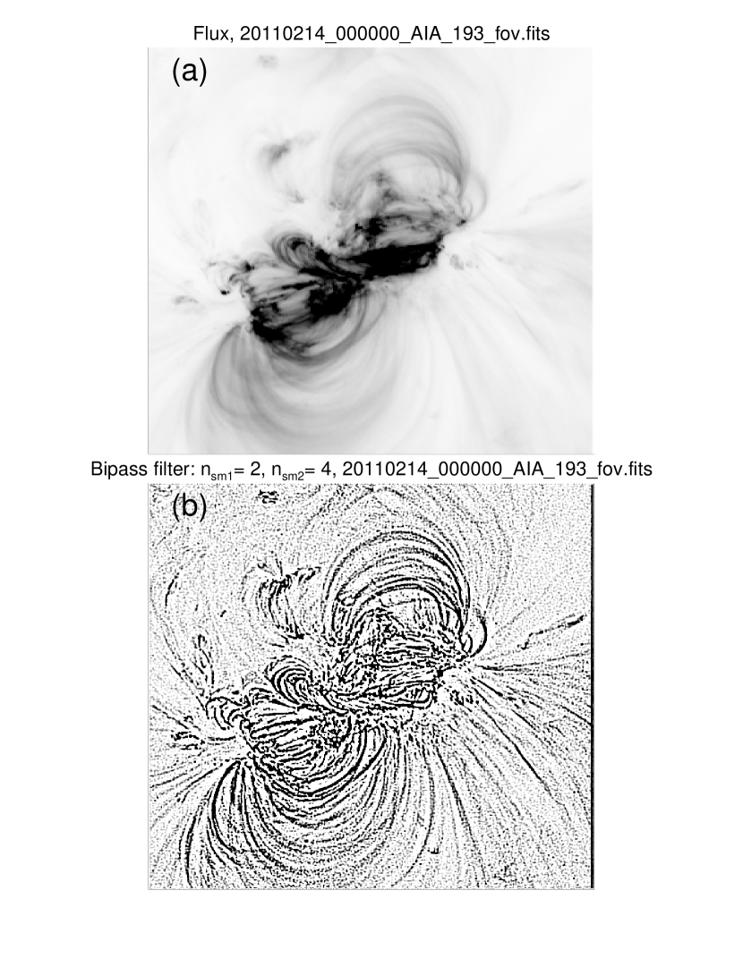
Figure 9: (a) EUV image observed with AIA/SDO on 2011-Feb-14, 00:00:00 UT, at a wavelength of 193 Å. The grey scale is inverted (black for bright emission) and the flux is rendered on a linear scale. (b): Bipass-filtered image with filters $n_{sm1}=1$ and $n_{sm2}=3$, which filters out structures with widths of $w=3\pm 1$. The image has a size of $486\times 486$ and a linear extent of 211 Mm.

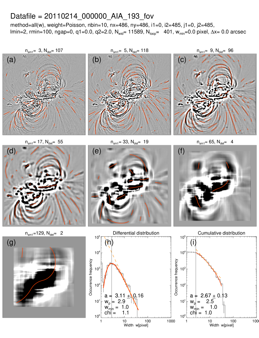
Figure 10: Seven bipass-filtered images (grey scale) with filters of $n_{sm1}=2,4,8,16,32,64,128$ pixels and automated loop tracings (red curves), obtained from the AIA/SDO image at a wavelength of 193 Å as shown in Fig. 9. Otherwise similar representation as in Fig. 6.

We analyze AIA images from 2011 February 14, 00:00 UT, in the six coronal wavelengths 94, 131, 171, 193, 211, and 335 Å. The AIA images have a full image size of 4096$\times$4096 pixels, with a pixel size of 0.6^′′, corresponding to a spatial resolution of $w_{res}=0.6\hbox{${}^{\prime\prime}$}\times 2.5$ pixels $\times$ 0.725 Mm $\approx$ 1.1 Mm on the solar surface). The time cadence of AIA is 12 s. For the automated pattern recognition we cut out a subimage with a field-of-view of 0.3 solar radii (or 487$\times$487 pixels), centered on the active region NOAA 11158, which has a heliographic position of S20 and E27 to W38 during the observed 6 days. One example is shown for 2011 Feb 14 in Figs. 9 and 10. The same active region is subject of over 40 published studies (for a list of references see Section 5.1.1. in Aschwanden, Sun, and Liu 2014). Descriptions of the SDO spacecraft and the AIA instrument can be found in Pesnell et al. (2011) and Lemen et al. (2012).

In each AIA image (at 6 wavelengths) we run the automated loop recognition code OCCULT-2 separately, sampling the number of loops ($n_{loop}$) and detected loop widths ($n_{wid}$), and performed power law fits for both the differential and cumulative size distributions. The results of the total number of detected loops $n_{loop}$, the power law slopes $a_{diff}$ and $a_{cum}$, and the goodness-of-fit $\chi^{2}$-values are listed in Table 1.

When we compare the results from AIA (Fig. 10) with those of our numerical simulation (Fig. 6), we find similar values for the power law slope $a\approx 3.1$, and the peak width $w_{p}\approx 2.9$ pixels, which confirms that our design of Monte-Carlo simulations closely reproduces the functional shape of the observed coronal loop width distributions. A new insight of this study is how the spatial resolution affects the occurrence frequency distribution $N(w)$ in the range from $w=1$ pixel to the peak of the size distribution of $w_{p}\lower 1.72218pt\hbox{$\;\buildrel<\over{\scriptstyle\sim}\;$}2.9$ pixels, which can be diagnosed from the normalized peak width value $w_{p}/\Delta x$.

For the power law slopes of the loop width distributions, averaged over all AIA wavelengths, we found mean values of $a_{diff}=2.7\pm 0.3$ and $a_{cum}=2.3\pm 0.4$ (Table 1), which corroborates the consistency between the differential and cumulative power law fitting method. The variation of the power law slope among different wavelengths is of order 10% (Table 1). The measured power law slopes $a$ can be understood as the fractal dimension of the geometric volume of an active region, because the simulated loop bundles are not space-filling, although the strands inside a loop bundle are space-filling. If an active region would be solidly filled with loops, we would expect a fractal dimension that corresponds to an Euclidean dimension of $a=D=3$. On the other side, if all detected loops are located in a 2-D layer with a fixed width in the third dimension, for instance caused by gravitational stratification, the expectation would be a Euclidean dimension of $a=D=2$. The fact that we find a power law index with a mean value $a\approx 2.7\pm 0.3$ indicates that the spatial distribution of measured loop cross-sections is fractal. In comparison, a fractal dimension of $D_{3}=2.0\pm 0.5$ has been inferred from 3-D modeling of 20 solar flare events (Aschwanden and Aschwanden 2008a,b).

5.2 Hi-C

We turn now to coronal images with the highest spatial resolution ever recorded, which were obtained during a rocket flight by the High-resolution Coronal Imager (Hi-C) on 2012 July 11. Instrumental descriptions are available from Kobayashi et al. (2014) and Cirtain et al. (2013). We use an image recorded at 18:54:16 UT, in the wavelength band of 193 Å, which is dominated by the Fe XII line originating around $T\approx 1.5$ MK. The image has a size of $3880\times 4096$ pixels, with a pixel size of $0.1\hbox{${}^{\prime\prime}$}$ (corresponding to 73 km/pixel), covering a field-of-view of 300 Mm ($\approx 0.37R_{\odot}$) squared, and was sampled with an exposure time of 2 s. The same image was analyzed previously by Peter et al. (2013).

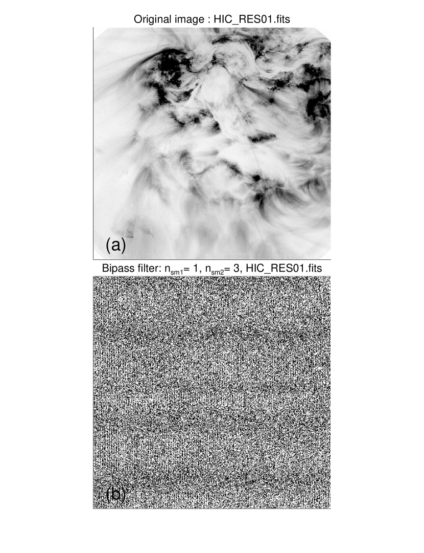
Figure 11: (a) EUV image observed with Hi-C on 2012-Jul-11, 18:54:16 UT, at a wavelength of 193 Å. The grey scale is inverted (black for bright emission) and the flux is rendered on a linear scale. (b): Bipass-filtered image with filters $n_{sm1}=1$ and $n_{sm2}=3$, which selects structures with a widths of $w\approx 140$ km. Note that the filtered image mostly shows random noise without any coherent loop strand structures.

We present the analyzed image in Fig. 11a, which contains a sunspot (in the upper half of the image), moss regions (in the upper left quadrant), as well as coronal loops in the periphery of an active region (bottom right quadrant), which are analyzed in Peter et al. (2013).

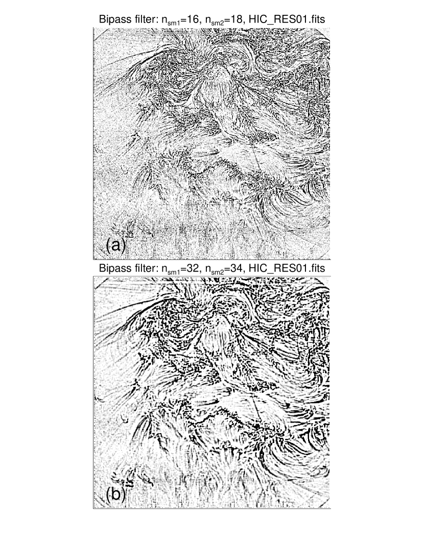
Figure 12: The same Hi-C image as shown in Fig. 9a, but filtered with $n_{sm1}=16$ and $n_{sm2}=18$, selecting structures with widths of $w\approx 1200$ km (a), and filtered with with $n_{sm1}=32$ and $n_{sm2}=34$, selecting structures with widths of $w\approx 2500$ km (b).

The structures hidden in the image can be enhanced by bipass filtering (Eq. 12), as revealed in Fig. 12a with a bipass filter of $n_{sm1}=16$ and $n_{sm2}=18$, which is most sensitive to structures with a width of $w=17\times 0.1\hbox{${}^{\prime\prime}$}\times 725$ km = 1200 km, or in Fig. 12b with a bipass filter of $n_{sm1}=32$ and $n_{sm2}=34$, which is most sensitive to structures with a width of $w=33\times 0.1\hbox{${}^{\prime\prime}$}\times 725$ km = 2400 km. However, filtering at the highest resolution, as shown in Fig. 11a with a bipass filter of $n_{sm1}=1$ and $n_{sm2}=3$, being most sensitive to structures with a width of $w=2\times 0.1\hbox{${}^{\prime\prime}$}\times 725$ km = 145 km, reveals no significant structures above the noise level anywhere (Fig. 11b), which is a surprising result that we will scrutinize in the following analysis in more detail.

In Fig. 13 we show the automated loop detection applied to the $3880\times 4096$ pixel full resolution HiC image, using the 7 bipass filters from $n_{sm1}=2$ to $n_{sm2}=128$. Almost no significant structure is seen at the highest resolution (Fig. 13a and 13b), while a maximum of $N_{det}=661$ structures is detected at the filter $n_{sm1}=32$ (Fig. 13e). The resulting size distribution of widths shows a peak width of $w_{p}/\Delta x=7.1$ pixels (Fig. 13h), which according to our numerical simulations is indicative of fully resolved width structures at the smallest scale of $w_{min}=1$ pixel or $0.1\hbox{${}^{\prime\prime}$}$, because we would expect a peak width of $w_{p}/\Delta x\approx 2.5$ for unresolved structures at full resolution.

5.3 Hi-C and AIA Comparisons

A comparison of the Hi-C image with the simultaneous and cospatial AIA image at the identical wavelength of 193 Å has been studied in Peter et al. (2013), from which we use the same images, which have been coaligned and corrected for a rotation of $1.9^{\circ}$. The only difference between these two images is the pixel size, with $0.1\hbox{${}^{\prime\prime}$}$ for Hi-C, and $0.6\hbox{${}^{\prime\prime}$}$ for AIA, being a factor of 5.8 different. AIA images have been taken 3 s before and 6 s after the Hi-C image. The results of our inter-comparison are tabulated in Table 2.

We perform an identical analysis of the AIA image (Fig. 14) as we did for the Hi-C image (Fig. 13). In the AIA image, significant structures are already visible at the full resolution (Fig 14a), which are comparable with those seen in the Hi-C image in the $n_{sm1}=17$ filter (Fig. 13d). Inspecting the size distribution of loop widths obtained in the AIA image, we find also a different peak width of $w_{p}/\Delta x=3.1$ (Fig. 14h), which indicates according to our numerical simulations that the finest structures are barely resolved in the AIA image at its full resolution ($0.6\hbox{${}^{\prime\prime}$}$), while they appear to be fully resolved in the Hi-C image at its full resolution ($0.1\hbox{${}^{\prime\prime}$}$).

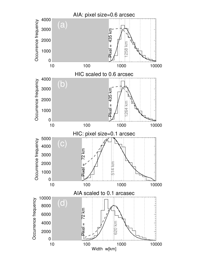
Figure 15: Comparison of width size distributions $N(w)$ (histograms) with fits of the model of Eq. 11 (solid curve), and corrected for finite resolutions (dashed curve), obtained with AIA (a), HiC scaled to AIA resolution (b), HiC (c), and AIA scaled to HiC resolution (d). The grey areas indicate width ranges where no structures can be resolved. The vertical dotted lines indicate the discrete width filters $n_{sm1}=2,4,8,...,128$.

In Fig. 15 we show a juxtaposition of the size distributions of the AIA image with an original pixel size of $0.6\hbox{${}^{\prime\prime}$}$ (Fig. 15a), the AIA image degraded to the Hi-C resolution of $0.1\hbox{${}^{\prime\prime}$}$ (Fig. 15d), the Hi-C image with the original pixel size of $0.1\hbox{${}^{\prime\prime}$}$ (Fig. 15c), and the Hi-C image re-scaled to the AIA resolution of $0.6\hbox{${}^{\prime\prime}$}$ (Fig. 15b). We find that the size distributions of widths are almost identical for equal pixel sizes, such as AIA and the rescaled Hi-C image with $0.6\hbox{${}^{\prime\prime}$}$ pixels (Figs. 15a and 15b), or the Hi-C and the rescaled AIA image with $0.1\hbox{${}^{\prime\prime}$}$ pixels (Figs. 15c and 15d). This means that there is essentially the same information stored for equal pixel sizes if all structures are resolved at this pixel size, which however would not be the case for unresolved structures. Further we find that rescaling of the same instrument does not preserve the peak width $w_{p}$, or the normalized peak width $w_{p}/\Delta x$, as it can be seen in the comparison of AIA (Fig. 15a) and the rescaled AIA (Fig. 15d), or in the comparison of Hi-C (Fig. 15c) and the rescaled Hi-C image (Fig. 15b). The results of this inter-comparison are summarized in Table 2. This is all consistent with our method that the peak width ratio $w_{p}/\Delta x$ can be used in the rescaling of the same image as a diagnostic for discriminating whether the finest structures in an image are resolved or not.

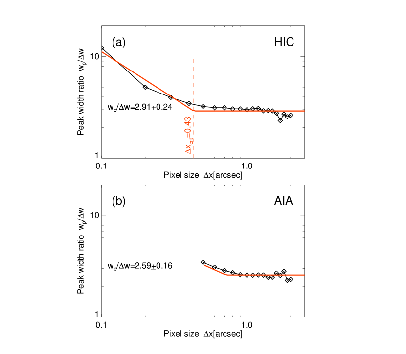
Figure 16: The peak width $w_{p}$ (of the width size distribution) is shown as a function of the pixel size $\Delta x\geq 0.1\hbox{${}^{\prime\prime}$}$ for the analyzed HI-C image (a), and for $\Delta x\geq 0.6\hbox{${}^{\prime\prime}$}$ for the simultaneously observed AIA image (b). At $w_{p}/\Delta x=3.0$, a minimum width of $\Delta x=0.77\hbox{${}^{\prime\prime}$}\approx 550$ km is found for the Hi-C image, below which loop structures are over-resolved with Hi-C. AIA resolves the structures at $\Delta x\lower 1.72218pt\hbox{$\;\buildrel<\over{\scriptstyle\sim}\;$}0.58\hbox{${}^{\prime\prime}$}$ = 420 km marginally.

In the results of the numerical simulations presented in Fig. 8, we demonstrated that the peak width ratio has a constant value of $w_{p}/\Delta x\approx 2.5$ for unresolved structures when the image is rescaled to different pixel sizes $\Delta x$, while the ratio increases to higher values at the highest resolution (of one pixel size) for images with fully resolved structures. For this experiment we rebin the Hi-C image from a pixel size of $\Delta x=0.1\hbox{${}^{\prime\prime}$}$ to $\Delta x=2.0\hbox{${}^{\prime\prime}$}$ in 20 equidistant steps of $\Delta x_{i}=0.1\times i,i=1,...,20$. Thus the rescaled image varies in the number of pixels from $3880\times 4096$ pixels down to $194\times 205$, but covers the same field-of-view and thus the same structures. We repeat for each of the 20 rescaled Hi-C images the automated pattern recognition algorithm and the sampling of width histograms, from which we extract the peak width ratio $w_{p}/\Delta x$ and plot it as a function of the pixel size $\Delta x$ (Fig. 16a). We find that the ratio is near-constant for large pixel sizes, while it increases to smaller pixel sizes. The separation point between fully resolved and unresolved loop widths can be read from the critical value $w_{p}/\Delta x=3.0$ on the y-axis, which yields a value of $\Delta x=0.77\hbox{${}^{\prime\prime}$}$ on the horizontal axis, corresponding to $w_{p}\approx 550$ km. Thus we conclude that the structures detected with Hi-C have the most frequent width value of $w_{p}\approx 550$ km, while thinner loop strands becoming rapidly sparser below this limit.

We repeat the same experiment with the AIA image for full-resolution (down to 1 pixel) and show the results in Fig. 16b. If we employ the same critial value of $w_{p}/\Delta x=3.0$ on the y-axis, we can read of a value of $\Delta x=0.58$ ^′′, which corresponds to $\Delta x=420$ km, which agrees with the value from Hi-C $\Delta x=550$ km within $\approx 25\%$. Thus, the AIA data indicate that all structures are mostly unresolved, but become marginally resolved at the full resolution of 1 AIA pixel, i.e., $\Delta x\approx 0.6\hbox{${}^{\prime\prime}$}$. Only with the additional information of Hi-C we can conclude that most structures are resolved below the AIA resolution.

The ratio of the detected (or observed) loop width $w$ to the true (or simulated) loop width $w_{true}$ follows from Eq. (4), i.e., $w=\sqrt{w_{true}^{2}+w_{min}^{2}}$, as visualized in Fig. 17. From Fig. 17 we can read off the ratio of the peak widths $w_{p}$ to the minimum width $w_{min}$, which is found to be $w_{p}/w_{min}=6.4$ for AIA, and $w_{p}/w_{min}=19.4$ for Hi-C, while we would expect a ratio of $w_{p}/w_{min}\approx 2.5$ for instruments that do not resolve the loop strands. Thus the diagram shown in Fig. 17 tells us that Hi-C fully resolves the bulk of loop strands, while AIA resolves most of them too, but only by a small margin compared with a non-resolving instrument.

6 DISCUSSION

6.1 Comparison with Previous Loop Width Measurements

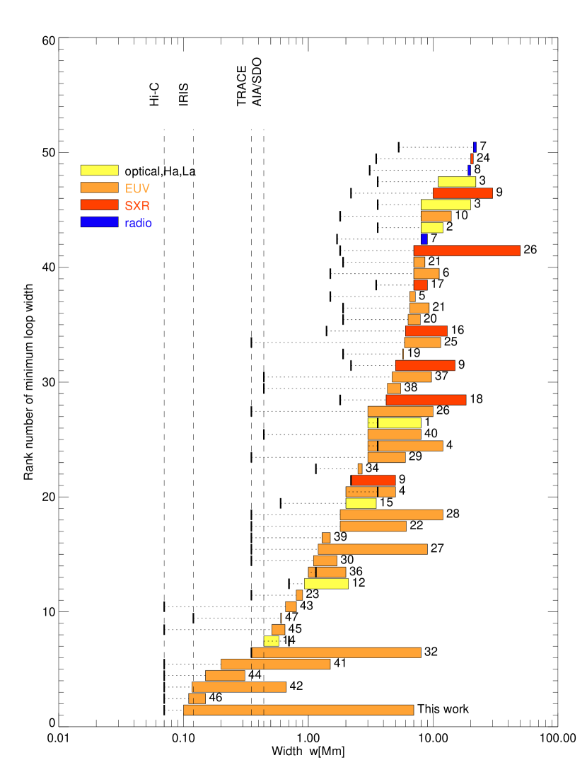
Figure 18: Compilation of loop width measurements from literature during 1963-2016: The measured ranges are represented by a block, colored by wavelength regimes (yellow=optical, H$\alpha$, L$\alpha$; orange=EUV, red=SXR, and blue=radio), labeled with the reference number given in Table 3, and sorted by the increasing minimum width on the y-axis. The instrumental pixel size (or resolution if pixel size is not known) is indicated with a black thick bar for each measurement. Automatically detected structures with widths of $w\lower 1.72218pt\hbox{$\;\buildrel>\over{\scriptstyle\sim}\;$}2$ Mm in this study are suspected to represent more complex structures than traditional loops.

We provide a comprehensive compilation of 52 studies that dealt with coronal loop width measurements in Table 3, with a graphical visualization in Fig. 18. Summaries of loop width measurements can also be found in Bray et al. (1991; Chapters 2 and 3), Aschwanden (1995), and Aschwanden (2004; Chapter 5.4.4). The graphical representation in Fig. 18 divides the loop width measurements in 4 wavelength regimes by color (optical + H$\alpha$ + Ly$\alpha$, EUV, soft X-rays, and radio), and ranks the width ranges by the smallest detected width in ascending order. There are several trends visible in this overview. Minimum loop widths have been measured from $w\approx 20$ Mm down to $w_{min}\approx 0.1$ Mm. The finest loop widths have been detected preferentially in EUV, while the loop widths measured in soft X-rays and optical wavelengths tend to be significantly larger, and are found to be largest in radio wavelengths. This can be explained because coronal loops in EUV and soft X-rays are produced by optically thin bremsstrahlung, which yields a better contrast than the partially optically thick free-free and gyroresonance emission in radio wavelengths.

In Table 3 we also list the pixel size $w_{pix}$ and the spatial resolution $w_{res}$ of the instruments. In Fig. 18 we can clearly see at one glance that the smallest loop widths are almost always measured a significant factor above the instrumental pixel sizes, which is partially explained by the point-spread function that typically amounts to 2.5 pixels in current EUV imagers (TRACE, AIA/SDO, STEREO, IRIS, Hi-C). Interestingly, the same ratio of $w_{p}/\Delta x\approx 2.5$ is also found in our present work, which corresponds to the optimum detection efficiency of our automated loop tracing algorithm (using bipass filters) in the case of the Monte-Carlo simulations, besides the effects of the point-spread function in the analyzed AIA and Hi-C data. Since every loop width measurement is subject to noise in the background, which causes some scatter in the order of a pixel size, for instance $w\approx 2.9\pm 1.1$ (pixels) in the example shown in Fig. 4. The lowest width measurements can be as low as $w\lower 1.72218pt\hbox{$\;\buildrel>\over{\scriptstyle\sim}\;$}1$ pixel using the equivalent-width method (Eq. 14). Some measurements shown in Fig. 18 exhibit even smaller widths than one pixel, because the authors attempted to determine the true width after deconvolution of the point-spread function, i.e., $w_{true}\approx\sqrt{w^{2}-w_{res}^{2}}$ (Eq. 4 and Fig. 17).

Virtually all studies that report loop width measurements are based on a single loop or a small number of visually selected (hand-picked) loops, which may contain the smallest features visible in an image, but they are not representative samples that would allow us to derive the entire width distribution of all coronal loops seen in an image. Our work thus represents a unique method that completely samples the entire size distribution function $N(w)dw$ over a range of about two orders of magnitude, characterized by the peak value ($w_{p}$), a smooth cutoff range $[w_{min},w_{p}]$ down to the minimum width value $(w_{min})$, and by a power law function in the upper part $[w_{p},w_{max}]$ up to the maximum size $(w_{max})$. Consequently, the range of loop widths measured in the present study ($w\approx 0.1-10$ Mm) entails all previous EUV measurements of loop widths, as it can be seen at one glance in Fig. 18.

However, we may ask whether the distribution of loop sizes continues at the low end if a future instrument faciliates a higher spatial resolution. Based on our peak width diagnostic criterion, this can only be the case if we measure a value of $w_{p}\approx 2.5\pm 0.2$ for the peak in the size distribution with the current highest-resolution instruments. The Hi-C measurements with 0.1^′′resolution, based on $n_{wid}=138,965$ individual loop width measurements (Fig. 13) indicate a peak width ratio of $w_{p}/\Delta x=7.1$ (Fig. 13h), which clearly suggests that most detected structures are fully resolved at $\Delta x=0.1\hbox{${}^{\prime\prime}$}$ resolution, while the most common loop width (which is given by the peak $w=w_{p}$ in the size distribution), amounts to $\Delta x=0.77\hbox{${}^{\prime\prime}$}$ (or $\Delta x\approx 550$ km; Fig. 16a). This does not exclude the possible measurement of smaller loops, but smaller loops are expected to be less common than loops with a mean width of $w_{p}\approx 550$ km, according to our criterion. Smaller loops have indeed been measured from recent Hi-C studies, e.g., $w=200-1500$ km (Peter et al. 2013), $w=117-667$ km (Brooks et al. (2013), $w=150-310$ km (Morton and McLaughlin 2013), or $w=120-150$ km (Brooks et al. (2016). Our prediction is that loops at $w\approx 550$ km are the most frequently occurring loops and form the peak of the size distribution, if sufficient spatial resolution is available, requiring $\Delta x\leq w_{p}/2.5\approx 120$ km (or $\approx 0.16\hbox{${}^{\prime\prime}$}$). This implies that a statistical analysis of IRIS data (De Pontieu et al. 2014) should be able to reproduce the peak at $w_{p}\approx 550$ km (or 0.77^′′). Most interestingly, Brooks et al. (2013) show an occurrence distribution of 91 hand-picked loops observed with Hi-C with a minimum Gaussian width of $\sigma_{w}=90$ km (FWHM=212 km) and an average Gaussian width of $\sigma_{w}=272$ km (FWHM=640 km), which is fully consistent with our result of a peak width (FWHM) of $w_{p}\approx 550$ km based on three orders of magnitude larger statistics. Winebarger et al. (2014) conducted a statistical analysis of the noise characteristics of a Hi-C image and concluded that 70% of the pixels in each Hi-C image do not show evidence for significant substructures, which confirms the scarcity of thinner loop strands than observed so far (see also Fig. 11b, where no structures except data noise is visible). Moreover, Peter et al. (2013) demonstrate that some of the loops seen in Hi-C are essentially resolved with AIA and appear to have a smooth Gaussian-like cross-section.

6.2 Consequences for Coronal Heating Models

There are two schools of coronal heating models: (1) The macroscopic view considers monolithic coronal loops that have heating cross-sections commensurable with the size of magneto-convection cells ($w\approx 300-1000$ km), and thus are mostly resolved with current EUV imagers (TRACE, AIA, IRIS, Hi-C); and (2) the microscopic view that postulates unresolved nanoflare strands that cannot be resolved with current instrumentation. Our continuously developing technology has faciliated tremendous improvements in astronomical high-resolution observations, so that the available spatial resolution improved by a factor of about 300 over the last 35 years. In particular, the measurement of coronal loop diameters improved from $w\approx 30$ Mm (Davis and Krieger 1982) down to $w\approx 0.1$ Mm with the current Hi-C observations (Peter et al. 2013; Brooks et al. 2013, 2016). Our new finding of a preferred spatial scale of $w_{p}\approx 550$ km for coronal loops calls for a physical explanation of this particular value. This peak width value $w_{p}$ separates the two regimes of a smooth cutoff range ($w<w_{p}$) and of a scale-free power law distribution at larger values ($w>w_{p}$).

One obvious physical scale is the granulation structure of the photosphere, discovered by Sir William Herschel in 1801. The spatial size of the time-varying granulation is measured by a combination of high-pass and low-pass filtering in the spatial frequency domain with subsequent thresholding, which segments granular and intergranular lanes. Alternative procedures are “lane-finding” schemes that are based on local gradient detection (Spruit et al. 1990). With the latter method, the smallest granules, near the observational limit, were found to have a most frequent size of 290 km. The size distribution peaks at $w_{p}=290$ km, then shows a slow decline in number up to a diameter near 1500 km, and then a rapid decline towards the largest granule sizes (Brandt 2001). Modern measurements with the New Solar Telescope at Big Bear, show a peak in the occurrence distribution of granule sizes shifted further down to $w\approx 150$ km (Abramenko et al. 2012).

If we adopt the magneto-convection of photospheric granular cells as the primary driver of local magnetic reconnection processes (in the chromosphere, transition region, and corona), for instance see numerical MHD simulations by Gudiksen et al. (2005) or Bingert and Peter (2013), we would expect a congruence between the magnetic reconnection area and the cross-sectional loop heating area (Aschwanden et al. 2007a,b). The diffusion region of a local magnetic reconnection process essentially defines the spatial scale of a local heating event, and therefore the cross-sectional area of a coronal loop. Our new result of a preferred cross-sectional scale of $w_{p}\approx 550$ km, which appears to be perfectly comparable with the most frequent granular scale, adds an additional constraint to the geometry of the heating process, besides ten other arguments that have been discussed earlier in the context of the coronal heating paradox (Aschwanden et al. 2007a,b).

The second school of thought deals with unresolved “microscopic” structures. The “nanoflare heating” scenario (Klimchuk 2006) builds on Parker’s (1988) conjecture that tangential misalignments of the magnetic field between adjacent flux tubes sporadically reconnect, driven by the braiding random motion of coronal loop footpoints in the photosphere. Since magneto-convection of the photosphere plays an important role as driver for magnetic braiding, which applies to both schools, the major difference between the monolithic and the nanoflare heating scenario is mostly the assumed spatial scale of the heating region, which contrasts the macroscopic view versus the microscopic view. There is a general consensus that broad loops are likely to consist of bundles of finer strands, as alluded to in Fig. 1, but the crucial question remains what the finest scale of a composite loop is. In the scale-free regime of a width distribution, a power-law like distribution function is generally observed that extends from $w_{max}$ down to the peak value $w_{p}$, where it breaks down by some unknown cutoff mechanisms. If nanoflares on finer scales exist, we would expect that the power law function extends to lower values than the observed cutoff, while the apparent peak width occurs at $w_{p}/\Delta x\approx 2.5$ due to the finite resolution. However, our crucial observation of $w_{p}/\Delta x\gg 2.5$ in Hi-C data contradicts this assumption that most frequent nanoflare strands exist at smaller spatial scales than $w<550$ km. This implies a physical limit, similar to the observed lower limit of granule sizes. Therefore we conclude that the Hi-C data are not consistent with a nanoflare scenario with most frequent loop strands at $w_{p}<550$ km. In addition, current nanoflare scenarios have difficulties to explain the isothermality of macroscopic loops (Aschwanden and Nightingale 2005; Aschwanden 2008), but see recent modifications in terms of “nanoflare storm” scenarios (Klimchuk 2015).

The best efforts to model Parker’s nanoflare scenario do not show a clear structuring across the (large-scale) magnetic field. In the turbulent (reduced) MHD model of Rappazzo et al. (2008) current sheets (along the large-scale magnetic field) form throughout the computational domain. No obvious structuring of the current sheets into bundles are found, where the heating is concentrated and which (in a more realistic model) could give rise to a coronal loop. So there is the need for an external process that would lead to a cross-field scale producing loops of finite width, and the photospheric magneto-convection is a good candidate for this.

6.3 Consequences for Coronal Density Measurements

Besides the consequences of loop width statistics on coronal heating models, there are numerous implications for coronal electron density measurements also. The emission measure of optically thin plasma, observed in EUV and soft X-rays, depends on the column depth, which is set equal to loop diameters for coronal loops with a circular cross-section. Thus, the density in coronal loops can only be determined if their diameter or width is known, such as SXT/Yohkoh measurements of soft X ray-bright flare loops (Aschwanden and Benz 1997). Therefore, measurements of coronal widths are essential for all theoretical models that require an electron density, such as calculations of the thermal energy, coronal filling factors, gyro-synchrotron emissivity, Alfvén speed, or coronal seismology. Such consequences will be discussed elsewhere.

7 CONCLUSIONS

In this study we explore the distribution of coronal loop widths with the AIA/SDO and the Hi-C instrument, which provide the highest spatial resolution available among current solar EUV imagers. Particular emphasis is given to the simultaneous data gathered during the Hi-C rocket flight on 2012 July 11. The scientific motivation for this study is the investigation of limits on the finest loop strands, which represent the “rosetta stone” of coronal heating models in discriminating microscopic (nanoflare strands) versus macroscopic (monolithic) loops. For this purpose we calculate analytical functions for the expected size distribution of loop widths, conduct numerical Monte-Carlo simulations to develop a diagnostic tool to discriminate whether the finest detected loop strands are spatially resolved or not, and analyze AIA and Hi-C data to apply this diagnostic tool to find fundamental limits on the smallest loop strands. We briefly summarize the results and conclusions in the following.

1. Automated loop detection: We apply the OCCULT-2 code for the automated detection of curvi-linear structures in EUV images from AIA and Hi-C. This code is able to measure $\approx 10^{5}$ loop widths in a Hi-C image. While previous loop widths have been measured only in small numbers and produced non-representative samples, this code allows us to obtain complete size distributions of loop widths, extending over two orders of magnitude, which was not possible with previous manual methods.

2. Principal Component Analysis: We applied bipass filters (consisting of a low-pass and high-pass filter), with a series of independent filter width components that increase by a factor of two over two orders of magnitude, which corresponds to orthogonal basis functions in principal component analysis methods. This range of spatial scales is suitable to reconstruct power law-like size distributions of loop widths.

3. The size distribution of loop widths: While no coronal loop model exists that predicts the size distribution of loop widths, we make use of the self-organized criticality approach, which predicts a power law function with a slope that depends on the (spatial) fractal dimension of a nonlinear energy dissipation system. We generalize the ideal power law function by including threshold effects and corrections due to finite instrumental spatial resolution. We introduce a smooth (lower) cutoff, which leads to a new analytical formulation of the size distribution function over the entire range $[w_{min},w_{max}]$, characterized by 4 free parameters: the minimum width $w_{min}$, the peak width $w_{p}$, the peak number $n_{0}$, and the power law slope $a$.

4. The peak width diagnostic: From Monte-Carlo simulations of EUV images with numerous loops that follow a prescribed power law distribution with a lower cutoff and random fluxes we explore how the peak width (or most frequently occurring width) $w_{p}$ depends on the lower cutoff in the width distribution of loop strands, using different pixel sizes $\Delta x$ (to mimic different spatial resolutions). We find that loop distributions that have a peak at $w_{p}/\Delta x\approx 2.5\pm 0.2$ contain unresolved strands, while larger width ratios indicate resolved structures at a pixel size $\Delta x$. In the case of resolved structures, we find a relationship between the minimum strand width $w_{min}$ and the critical resolution $\Delta x$ that separates the two regimes of resolved and unresolved loop widths, i.e., $w_{p}/\Delta x=3.0$, which can be used to diagnose the lower cutoff of a completely sampled loop width distribution.

5. Marginally resolved loop widths with AIA: The AIA 193 Å image rescaled to pixel sizes ranging from $0.6\hbox{${}^{\prime\prime}$}$ to $20.0\hbox{${}^{\prime\prime}$}$ yields size distributions of loop cross-section widths that have a peak at an invariant ratio of $w_{p}/\Delta x=2.59\pm 0.16$, while a slightly higher value is obtained near the full resolution, which indicates according to our numerical simulations that the structures are marginally resolved at the full resolution of $\Delta x=0.6\hbox{${}^{\prime\prime}$}$, and that the most frequent value of the loop size distribution has a value of $w_{min}\lower 1.72218pt\hbox{$\;\buildrel>\over{\scriptstyle\sim}\;$}420$ km.

6. Resolved loop widths with Hi-C: The Hi-C 193 Å image that was observed simultaneously with the AIA 193 Å image, sampled at full resolution of $\Delta x=0.1\hbox{${}^{\prime\prime}$}$, yields a size distribution of loop widths peaking at $w_{p}/\Delta x=7.1$, which indicates according to our numerical simulations that all structures are over-resolved at the full resolution. When we re-scale the Hi-C image in the range of $\Delta x=0.1\hbox{${}^{\prime\prime}$}-20.0\hbox{${}^{\prime\prime}$}$, we find a most frequent loop width of $\Delta x\approx 550$ km.

7. Comparison with previous loop measurements: We identified 52 studies that contain loop width measurements, observed in optical, H$\alpha$, Ly$\alpha$, soft X-rays (SXR), extreme ultra-violet (EUV), and radio wavelengths, which report values over a range of $w=0.1-30$ Mm. All previous measurements were carried out on single loops or a small number of loops, while this study samples for the first time loop cross-sections over a scale range of two orders of magnitude in each image. The finest loop widths have been detected with IRIS and Hi-C have a lower limit of $w_{min}\lower 1.72218pt\hbox{$\;\buildrel>\over{\scriptstyle\sim}\;$}100$ km and a peak value of the most frequently observed (resolved) loop width of $w_{p}\approx 550$ km. The closest confirmation is the Hi-C study of Brooks et al. (2013), which shows 91 loops with a low cutoff of $w\lower 1.72218pt\hbox{$\;\buildrel>\over{\scriptstyle\sim}\;$}200$ km and a peak at $w_{p}\approx 640$ km.

8. Consequences for coronal heating models: The coronal loop widths inferred here, with a peak value of $w_{p}\approx 550$ km and a minimum of $w_{min}\approx 100$ km agrees with the size of the most frequently occurring granule sizes in the photosphere. We conclude that this geometric congruence supports coronal heating models that are driven by photospheric magneto-convection and operate most frequently on a macroscopic scale of $w\approx 550$ km, rather than nanoflare heating models that involve unresolved loop strands beyond the spatial resolution of current instrumentation.

This is the first study that finds an absolute lower limit on the width of coronal loops, based on automated measurements with large statistics, from which the size distribution of loop widths can be sampled and diagnostic criteria can be derived that are capable to distinguish whether the finest loops observed in a high-resolution image are resolved or not, for a given instrument. Since a size distribution contains much more information than a single case measurement, this statistical approach with automated loop detection and size distribution modeling offers more powerful tools to test coronal heating models than previous single point measurements, which all are not representative samples of the entirity of all coronal loops. If the inferred absolute lower limit on loop widths holds up in complementary future studies, we may conclude that we are hitting the rock bottom of loop width sizes. A major consequence may be the irrelevance of (hypothetical) unresolved nanoflare structures.

Table 1: Measurement of the power law slope of loop width distribution functions obtained in different wavelengths of the AIA image of 2011 Feb 14, 00:00 UT: The number of detected loops $n_{loop}$, measured widths $n_{wid}$, the power law slope of the differential frequency distribution $a_{diff}$, and of the cumulative frequency distribution $a_{cum}$, and the goodness-of-fit values $\chi_{diff}$ and $\chi_{cum}$.

Wave	Number	Number	Power law	Power law	Goodness	Goodness
length	of loops	of widths	slope	slope	of fit	of fit
	$n_{loop}$	$n_{wid}$	$a_{diff}$	$a_{cum}$	$\chi_{diff}$	$\chi_{cum}$
[Å]
94	80	2653	2.5$\pm$0.3	1.8$\pm$0.2	0.8	1.0
131	199	5796	2.7$\pm$0.2	2.6$\pm$0.2	1.0	2.2
171	463	15017	2.7$\pm$0.1	2.8$\pm$0.1	1.1	1.9
193	401	11589	3.1$\pm$0.2	2.7$\pm$0.1	1.1	1.0
211	310	9232	2.7$\pm$0.2	2.2$\pm$0.1	0.8	2.7
335	125	3871	2.4$\pm$0.2	1.9$\pm$0.2	0.8	1.1
Mean			2.7$\pm$0.3	2.3$\pm$0.4

Table 2: Measurement of the power law slope of loop width distribution functions obtained from simultaneous HiC and AIA 193 A images scaled to each others pixel size: the number of detected loops $n_{loop}$, measured widths $n_{wid}$, the normalized peak width $w_{p}/\Delta x$, the power law slope of the differential frequency distribution $a_{diff}$, and of the cumulative frequency distribution $a_{cum}$, and the goodness-of-fit values $\chi_{diff}$ and $\chi_{cum}$.

Instrument	Pixel	Number	Number	Peak	Power law	Power law	Goodness	Goodness
	size	of loops	of widths	width	slope	slope	of fit	of fit
		$n_{loop}$	$n_{wid}$	$w_{p}$	$a_{diff}$	$a_{cum}$	$\chi_{diff}$	$\chi_{cum}$
	(arcsec)
AIA	0.6	784	20,927	3.1	2.6$\pm$0.1	2.2$\pm$0.1	1.7	1.3
HIC & AIA pixels	0.6	770	20,629	2.9	2.6$\pm$0.1	2.3$\pm$0.1	1.7	1.7
HIC	0.1	2459	138,965	7.1	1.4$\pm$0.1	2.0$\pm$0.1	1.5	4.8
AIA & HIC pixels	0.1	3205	188,926	8.3	2.7$\pm$0.1	2.5$\pm$0.1	…	…
Mean					2.3$\pm$0.6	2.3$\pm$0.2

Table 3: Compilation of coronal loop width measurements in chronological order.

Object	Pixel	Spatial	Loop	Wavelength	Instrument	Ref.
	size	resolution	width
	$w_{pix}$ [Mm]	$w_{res}$ [Mm]	$w_{loop}$ [Mm]	$\lambda$ [Å]
green corona loops	…	…	$3-8$	5303	Dunn/SacPeak	1
large green corona loops	…	…	$8-12$	5303	Dunn/SacPeak	2
green corona loops	…	3.6	$11-22$	5303	Pic-du-Midi	3
red corona structures	…	3.6	$8-20$	6374	Pic-du-Midi	3
cool loops	…	3.6	$2-5$	1032 O VI	Skylab	4
cool loops	…	3.6	$<2$	465 Ne VII	Skylab	4
hot loops	…	3.6	$3-12$	1032 Mg X	Skylab	4
hot loops	…	3.6	$3-12$	465 Si XII	Skylab	4
loop prominence	…	1.5	$6.5-7.2$	160-630	Skylab	5
active region loop	…	1.5	$7-11$	Fe XVI	Skylab	6
radio loop structure	…	5.3	$22$	11 cm	NRAO	7
radio loop structure	…	1.7	$9$	3.7 cm	NRAO	7
active region loops	…	3.1	$20$	20 cm	VLA	8
active region core loops	2.2	…	$<2.2-5$	SXR	ASE rocket	9
compact volume loops	2.2	…	$5-15$	SXR	ASE rocket	9
outward extending loops	2.2	…	$10-30$	SXR	ASE rocket	9
hot coronal loops	…	1.8	$8-14$	170-630	Skylab	10
coronal loops	…	3.1	$16-20$	20 cm	VLA	11
active region loops	…	0.7	$0.93-2.1$	H$\alpha$	CSIRO	12,13
very thin loops (chrom)	…	0.7	$0.44-0.58$	H$\alpha$	CSIRO	14
very thin loops (photo)	…	0.7	$<0.13-0.32$	H$\alpha$	CSIRO	14
coronal loops	0.6	0.7	$2-3.5$	Ly$\alpha$	LMSAL rocket	15
X-ray loops	…	1.4	$6-13$	8-65	ASE rocket	16
soft X-ray loops	3.5	…	$7-9$	SXR	SXT/Yohkoh	17
soft X-ray flare loops	…	1.8	$4.2-18.4$	SXR	SXT/Yohkoh	18
active region loop	1.9	…	$5.8$	171, 195	EIT/SOHO	19
active region loops	1.9	…	$7.1\pm 0.8$	171	EIT/SOHO	20
active region loops	1.9	…	$7.8\pm 0.8$	195	EIT/SOHO	21
active region loops	1.9	…	$7.9\pm 1.4$	284	EIT/SOHO	21
nanoflare loops	0.35	0.82	$1.8-6.1$	171, 195	TRACE	22
postflare arcade loops	0.35	0.82	$0.9$	171, 195	TRACE	23
soft X-ray loop	3.5	…	$21$	SXR	SXT/Yohkoh	24
oscillating loops	0.35	0.82	$8.7\pm 2.8$	171, 195	TRACE	25
nanoflare loops	0.35	0.82	$3-10$	171, 195	TRACE	26
nanoflare loops	…	1.8	$7-50$	SXR	SXT/YOHKOH	26
oscillating loops	0.35	0.82	$5.1\pm 3.9$	171, 195	TRACE	27
cooling loops	0.35	0.82	$1.8-12.0$	171, 195	TRACE	28
heated loop	0.35	0.82	$3-6$	171, 195	TRACE	29
elementary loops	0.35	0.82	$1.4\pm 0.3$	171, 195, 284	TRACE	30,31
cool $(<0.1$ MK) loops	0.09	0.22	$0.7-2.2$	1216	VAULT	32
cooling loops	0.35	0.82	$<0.35-8.0$	171, 195	TRACE	33
3D-reconstructed loops	1.15	2.30	$2.6\pm 0.1$	171,195,284	EIT/STEREO	34,35
coronal loops	0.35	0.82	$0.7-2.2$	171,195	TRACE	36
3D-reconstructed loops	1.15	2.30	$<1.0\pm 1.0$	171,195,284	EIT/STEREO	37
coronal loops	0.44	0.98	$4.7-9.7$	94-335	AIA/SDO	38
oscillating loop	0.44	0.98	$4.9\pm 0.6$	94-335	AIA/SDO	39
cooling loops	0.35	0.82	$1.29-1.50$	171, 195	TRACE	40
coronal loops	0.73	…	$0.7-1.9$	195	EIS/Hinode	41
coronal rain	0.06	0.14	$0.31$	6563	CRISP	42
auto-detected loops	0.44	0.98	$3-8$	94-335	AIA/SDO	43
coronal loops	0.07	0.22	$0.2-1.5$	193	Hi-C	44
coronal loops	0.07	0.22	$0.117-0.667$	193	Hi-C	45
inter-moss loops	0.07	0.22	$0.675-0.803$	193	Hi-C	46
oscillating loops	0.07	0.22	$0.15-0.31$	193	Hi-C	47
filament threads	0.07	0.22	$0.58\pm 0.07$	193	Hi-C	48
finely structured corona	0.07	0.22	$>0.22$	193	Hi-C	49
coronal rain	0.06	0.14	$0.15-0.28$	6563	CRISP	50
coronal rain	0.08	0.15	$0.32-0.57$	3968	SOT/Hinode	50
coronal rain	0.12	0.30	$0.44-0.72$	2796	IRIS	50
coronal rain	0.12	0.30	$0.40-0.62$	1330	IRIS	50
coronal rain	0.12	0.30	$0.46-0.70$	1400	IRIS	50
coronal rain	0.44	0.98	$1.02-1.24$	304	AIA/SDO	50
coronal rain	0.44	0.98	$0.51-1.52$	304	AIA/SDO	50
coronal rain	0.44	0.98	$1.19-2.36$	171	AIA/SDO	50
coronal rain	0.44	0.98	$1.17-2.73$	193	AIA/SDO	50
fine structure loops	0.12	0.30	$0.12-0.15$	1400	IRIS	51
penumbral jets	0.07	0.22	$<0.6$	193	Hi-C	52

Figure 2: (a) Analytical function of an ideal power law (thin solid line), a thresholded power law with a threshold $x_{0}/w_{min}=2.5$ (dashed curve), a thresholded power law with a finite spatial resolution $w_{\mathrm{min}}$ (dash-dotted curve), and a power law function with a smooth cutoff peaking at $w_{p}/w_{min}=2.5$ according to Eq. 11 (thick solid line). The minimum value at $w_{min}$ and the sampling threshold at $x_{0}/w_{min}=2.5$ are indicated with vertical dotted lines. (b) A family of power law functions with smooth cutoffs and peaks at $w_{p}/w_{min}=1,2,...,20$ (Eq. 11).

Figure 3: The geometry of automated curvi-linear feature tracking is shown, starting at a local flux maximum location $(x_{0},y_{0})$, where the linear direction of the local ridge is measured (angle $\alpha$) and a set of circular segments within a range of curvature radii is fitted to the local ridge (thick linestyle). The locations $(xr_{i},yr_{i}),i=0,...,19$ mark the centers of the curvature radii (Aschwanden, De Pontieu, and Katrukha 2013a).

Figure 17: Detected (or observed) loop width ratio $w_{p}/w_{min}$ as a function of simulated (or true) loop widths $w_{true}$ are shown, simulated with different true loop widths $w_{true}$. The diamonds represent the ratios of the peak widths $w_{p}$ to the minimum widths $w_{min}$ of seven simulated width distributions. The horizontal line indicates the limit of spatially unresolved structures, which yields an asymptotic value of $w_{p}/w_{min}\approx 2.5\hbox{${}^{\prime\prime}$}$. The dotted line indicates equivalence between simulated and detected loop widths. The dashed line indicates the relationship $w_{det}=\sqrt{w_{true}^{2}+w_{min}^{2}}$ (Eq. 4).

References

- (1)
- (2)
- (3) Abramenko, V.I., Yurchyshyn, V.B., Goode, P.R., Kitiashvili, I.N., and Kosovichev, A.G. 2012, ApJ 756, L27.
- (4) Alexander, C.E., Walsh, R.W., Regnier, S., Cirtain, J., Winebarger, A.R., Golub, L., Kobayashi, K., Platt, S., et al. 2013, ApJ 775, L32.
- (5) Amendt, P. and Benford, G. 1989, ApJ 341, 1082.
- (6) Antolin, P., Vissers, G., Pereira, M.D., Rouppe van der Voort, L., Scullion, E. 2015, ApJ 806, 81.
- (7) Antolin, P. and Rouppe van der Voort, L. 2012, 745, 152.
- (8) Arregui, I. and Asensio-Ramos, A. 2014, A&A 565, A78.
- (9) Arregui, I., Soler, R., and Asensio Ramos, A. 2015, ApJ 811, 104.
- (10) Aschwanden, M.J. 1995, Lecture Notes in Physics, 444, 13.
- (11) Aschwanden, M.J. and Benz, A.O. 1997, ApJ 480, 825.
- (12) Aschwanden, M.J., Neupert, W.N., Newmark, J., Thompson,B.J., Brosius, J.W., Holman, G.D., Harrison, R.A., Bastian, T.S., et al. 1998, in Proc. ”Three-Dimensional Structure of Solar Active Regions”, (eds. C.Alissandrakis and B.Schmieder), ASP: San Francisco, ASP Conf. Ser. Vol. 155, 145.
- (13) Aschwanden, M.J., Newmark, J.S., Delaboudiniere, J.P., Neupert, W.M., Klimchuk, J.A., Gary, G.A., Portier-Fornazzi, F., and Zucker,A. 1999, ApJ 515, 842.
- (14) Aschwanden, M.J., Alexander, D., Hurlburt, N., Newmark, J.S., Neupert, W.M., Klimchuk, J.A., and G.A. Gary 2000a, ApJ 531, 1129.
- (15) Aschwanden, M.J., Tarbell, T., Nightingale, R., Schrijver, C.J., Title, A., Kankelborg, C.C., Martens, P.C.H., and Warren, H.P. 2000b, ApJ 535, 1047.
- (16) Aschwanden, M.J., Nightingale, R.W., Tarbell, T.D., and Wolfson, C.J., 2000c, ApJ 535, 1027.
- (17) Aschwanden, M.J. and Alexander, D. 2001, Solar Phys. 204, 93.
- (18) Aschwanden, M.J. 2002, in Proc. Multi-Wavelength Observations of Coronal Structure and Dynamics, COSPAR Colloquia Series, Vol. 13, (eds. Martens,P.C.H. and Cauffman,D.), Elsevier Science: Amsterdam, 57.
- (19) Aschwanden, M.J., DePontieu, B., Schrijver, C.J., and Title, A. 2002, Solar Phys. 206, 99.
- (20) Aschwanden, M.J. and Parnell,C.E. 2002, ApJ 572, 1048.
- (21) Aschwanden, M.J., Nightingale, R.W., Andries, J., Goossens, M., and Van Doorsselaere, T. 2003a, ApJ 598, 1375.
- (22) Aschwanden, M.J., Schrijver, C.J., Winebarger, A.R., and Warren, H.P. 2003b, ApJ 588, L49.
- (23) Aschwanden, M.J. 2004, Physics of the Solar Corona - An Introduction, Springer, New York, ISBN 3-540-22321-5.
- (24) Aschwanden, M.J. and Nightingale, R.W. 2005, ApJ 633, 499.
- (25) Aschwanden, M.J., Nightingale, R.W., and Boerner, P. 2007a, ApJ 656, 577.
- (26) Aschwanden, M.J., Winebarger, A., Tsiklauri, D., and Peter, H. 2007b, ApJ 659, 1673.
- (27) Aschwanden, M.J. and Aschwanden, P.D. 2008a, ApJ 674, 530.
- (28) Aschwanden, M.J. and Aschwanden, P.D. 2008b, ApJ 674, 544.
- (29) Aschwanden, M.J. and Terradas, J. 2008, ApJ 686, L127.
- (30) Aschwanden, M.J. 2008, ApJ 672, L135.
- (31) Aschwanden, M.J., Wuelser, J.P., Nitta, N., and Lemen, J. 2008a, ApJ 679, 827.
- (32) Aschwanden, M.J., Nitta, N.V., Wuelser, J.P., and Lemen, J.R. 2008b, ApJ 680, 1477.
- (33) Aschwanden, M.J., Lee, J.K., Gary, G.A., Smith, M., and Inhester,B. 2008c, Solar Phys. 248, 359.
- (34) Aschwanden, M.J. 2010, Solar Phys. 262, 399.
- (35) Aschwanden, M.J. and Boerner, P. 2011, ApJ 732, 81.
- (36) Aschwanden, M.J. and Schrijver, C.J. 2011, ApJ 736, 102.
- (37) Aschwanden, M.J. 2011, Self-Organized Criticality in Astrophysics. The Statistics of Nonlinear Processes in the Universe, Springer-Praxis, New York.
- (38) Aschwanden, M.J. and Wülser, J.P. 2011, JASTP 73, 1082.
- (39) Aschwanden, M.J. and Schrijver, C.J. 2011, ApJ 736, 102.
- (40) Aschwanden, M.J. 2012, A&A 539, A2.
- (41) Aschwanden, M.J., DePontieu, B., and Katrukha, E. 2013a, Entropy, 15(8), 3007.
- (42) Aschwanden, M.J., Boerner, P., Schrijver, C.J., and Malanushenko, A. 2013b, Solar Phys. 283, 5.
- (43) Aschwanden, M.J. 2014, ApJ 782, 54.
- (44) Aschwanden, M.J., Sun, X.D., and Liu, Y. 2014, ApJ 785, 34.
- (45) Aschwanden, M.J. 2015, ApJ 814, 19.
- (46) Aschwanden, M.J., Crosby, N., Dimitropoulou, M., Georgoulis, M.K., Hergarten, S., McAteer, J., Milovanov, A., Mineshige, S., et al. 2016, Space Science Reviews 198, 47.
- (47) Bak, P., Tang, C., and Wiesenfeld, K. 1987, PhRvL 59/4, 381.
- (48) Bellan, P.M. 2003, AdSpR 32(10), 1923.
- (49) Berger, T.E., De Pontieu, B., Fletcher, L., Schrijver, C.J., Tarbell, T.D., and Title, A.M. 1999, Solar Phys. 190, 409.
- (50) Bian, N.H., Kontar, E.P. and MacKinnon, A.L. 2011, A&A 535, A130.
- (51) Bingert, S. and Peter, H. 2013, A&A 550, A30.
- (52) Brandt, P.N. 2001, in Encyclopedia of Astronomy and Astrophysics, (ed. Paul Murdin), Institute of Physics Publishing Group: New York.
- (53) Bray, R.J. and Loughhead, R.E. 1985, A&A 142, 199.
- (54) Bray, R.J., Cram, L.E., Durrant, C.J., and Loughhead, R.E. 1991, Plasma loops in the solar corona, Cambridge University Press: Cambridge.
- (55) Brooks, D.H., Warren, H.P., and Ugarte-Urra, I. . 2012, ApJ 755, L33.
- (56) Brooks, D.H., Warren, H.P., Ugarte-Urra, I., and Winebarger, A.R. 2013, ApJ 772, L19.
- (57) Brooks, D.H., Reep, J.W., and Warren, H.P., 2016, ApJ 826, L18.
- (58) Cadavid, A.C., Lawrence, J.K., and Ruzmaikin, A. 2008, Solar Phys. 248, 247.
- (59) Casini,R., Bevilacqua, R., and Lopez-Ariste, A. 2005, ApJ 622, 1265.
- (60) Chae, J., Poland, A.I., and Aschwanden, M.J. 2002, ApJ 581, 726.
- (61) Cheng, C.C. 1980, Solar Phys. 65, 347.
- (62) Cheng, C.C., Smith, J.B., and Tandberg-Hanssen, E. 1980, Solar Phys. 67, 259.
- (63) Cirtain, J.W., Golub, L., WInebarger, A.L., et al. 2013, Nature, 493, 501.
- (64) Clauset, A., Shalizi, C.R., and Newman, M.E.J. 2009, SIAM Rev. 51/4, 661.
- (65) Davis, J.M. and Krieger, A.S. 1982, Solar Phys. 80, 295.
- (66) De Pontieu, B., Title, A.M., Lemen, J.R., Kushner, G.D., Akin, D.J., Allard, B., Berger, T., Boerner, P., et al. 2014, Solar Physics 289, 2733.
- (67) Dere, K.P. 1982, Solar Phys. 75, 189.
- (68) Dunn, R.B. 1971, in “Physics of the Solar Corona”, (ed. C.J. Macris), Reidel: Dordrecht, Vol. 24, 114.
- (69) Erdelyi, R. and Morton, R.J. 2009, A&A 494, 295.
- (70) Foukal, P. 1975, Solar Phys. 43, 327.
- (71) Galloway, R.K., Helander,P.M. and MacKinnon, A.L. 2006, ApJ 646, 615.
- (72) Georgoulis, M.K., and LaBonte, B.J. 2004, ApJ 615, 1029.
- (73) Golub, L., Bookbinder, J., DeLuca, E., Karovska, M., Warren,H., Schrijver, C.J., Shine, R., Tarbell, T. et al. 1999, Physics of Plasmas 6/5, 2205.
- (74) Gudiksen, B.V. and Nordlund, A. 2005, 618, 1031.
- (75) Jackson, J.E. 2003, A User’s Guide to Principal Components, Wiley, Hoboken.
- (76) Kaneko, T., Goossens, M., Soler, R., Terradas, J., Van Doorsselaere, T., Yokoyama, T., and Wright, A.N., 2015, ApJ 812, 121.
- (77) Kleczek, J. 1963, PASJ 75, 9.
- (78) Klimchuk, J.A., Lemen, J.R., Feldman, U., Tsuneta, S., Uchida, Y. 1992, PASJ 44, L181.
- (79) Klimchuk, J.A. 2006, Solar Pnys. 234, 41.
- (80) Klimchuk, J.A. 2000, Solar Phys. 193, 53.
- (81) Klimchuk, J.A. 2015, Royal Soc. London Phil. Trans. Ser. A, 373, 40256.
- (82) Kobayashi, K., Cirtain, J., Winebarger, A. R., Korreck, K., Golub, L., Walsh, R. W., De Pontieu, B., DeForest, et al. 2014, Solar Phys., 289, 4393.
- (83) Kontar, E.P., Hannah, I.G., and Bian,N.H. 2011, ApJ 730, L22.
- (84) Kundu, M.R., Schmahl, E.J., Gerassimenko, M. 1980, A&A 82, 265.
- (85) Kundu, M.R. and Velusamy T. 1980, ApJ 240, L63.
- (86) Lang, K.R., Willson, R.F., and Rayrole, J. 1982, ApJ 258, 384.
- (87) Lawrence, J.K., Cadavid, A., and Ruzmaikin, A. 2004, Solar Phys. 225, 1.
- (88) Lemen, J.R., Title, A.M., Akin, D.J., Boerner, P.F., Chou, C., Drake, J.F., Duncan, D.W., Edwards, C.G., et al. 2012, Solar Phys. 275, 17.
- (89) Lomax, K.S. 1954, J. American Statistical Association 49, 847.
- (90) Lopez-Fuentes, M.C., Demoulin, P., and Klimchuk, J.A. 2008, ApJ 673, 586.
- (91) Lopez-Fuentes, M.C. and Klimchuk, J.A. 2010, ApJ 799, 128.
- (92) Loughhead, R.E. and Bray, R.J. 1984, ApJ 283, 392.
- (93) Loughhead, R.E., Bray, R.J., and Wang, J.-L. 1985, ApJ 294, 697.
- (94) Morton, R.J. and Ruderman, M.S. 2011, A&A 527, A53.
- (95) Morton, R.J. and McLaughlin, J.A. 2013, A&A 553, L10.
- (96) Mulu-Moore, F.M., Winebarger, A.R., Warren, H.P., and Aschwanden, M.J. 2011, ApJ 733, 59.
- (97) Parker, E.N. 1988, ApJ 330, 474.
- (98) Pascoe, D.J., Nakariakov, V.M., Arber, T.D., and Murawski, K. 2009, A&A 494, 1119.
- (99) Patsourakos, S., and Klimchuk, J.A. 2007, ApJ 667, 591.
- (100) Patsourakos, S., Gouttebroze, P., and Vourlidas, A. 2007, ApJ 664, 1214.
- (101) Pesnell, W.D., Thompson, B.J., and Chamberlin, P.C. 2011, SP 275, 3.
- (102) Peter, H., and Bingert, S. 2012, A&A 548, A1.
- (103) Peter, H., Bingert, S., Klimchuk, J.A., de Forest, C., Cirtain, J.W., Golub, L., WInebarger, A.R., Kobayashi, K., and Korreck, E., 2013, A&A 556, id. A104.
- (104) Petrie, G.J.D., Gontikakis, C., Dara, H., Tsinganos, K., and Aschwanden, M.J. 2003, A&A 409, 1065.
- (105) Petrie, G.J.D. 2006, ApJ 649, 1078.
- (106) Picat, J.P., Fort, B., Dantel, B., and Leroy, J.L. 1973, A&A 24, 259.
- (107) Rappazano, A.F., Velli, M., Einaudi, G., Dahlburg, R.B. 2008, ApJ 677, 1348.
- (108) Ruderman, M.S. 2003, A&A 409, 287.
- (109) Ruderman, M.S., Verth, G., and Erdelyi, R. 2008, ApJ 686, 694.
- (110) Ruderman, M.S. 2015, Solar Phys. 290, 423.
- (111) Schmelz, J.T., Pathak, S., Jenkins, B.S., and Worley, B.T. 2013, ApJ 764, 53.
- (112) Schrijver, C.J. 2007, ApJ 662, L119.
- (113) Spruit, H.C., Nordlund, A., and Title, A.M. 1990, Ann. Rev. Astron. Astrophys. 28, 263.
- (114) Tiwari, S.K., Moore, R.L., Winebarger, A.R., and Alpert, S.E. 2016, ApJ 816, 92.
- (115) Tsiropoula, G., Alissandrakis, C., Bonnet, R.M., and Gouttebroze, P. 1986, A&A 167, 351.
- (116) Vasquez, B.J. and Hollweg, J.V. 2004, GRL 31, 4803.
- (117) Voitenko, Y.M. and Goossens, M. 2004, ApJ 605, L149.
- (118) Voitenko, Y.M. and Goossens, M. 2005, PhRL 94, 135003.
- (119) Wang, H. and Sakurai, T. 1998, PASJ 50, 111.
- (120) Watko, J.A. and Klimchuk, J.A. 2000, Solar Phys. 93, 77.
- (121) Webb, D.F., Holman, G.D., Davis, J.M., Kundu, M.R., and Shevgaonkar, R.K. 1987, ApJ 315, 716.
- (122) Winebarger, A.R., Walsh, R.W., Moore, R., De Pontieu, B., Hansteen, V., Cirtain, J., Golub, L., Kobayashi, K. et al. 2013, ApJ 771, 21.
- (123) Winebarger, A.R., Cirtain, J., Golub, L., DeLuca, E., Savage, S., Alexander, C., and Schuler, T. 2014, ApJ 787, L10.
- (124) Winglee, R.M., Dulk, G.A., and Pritchett, P.L. 1988, ApJ 328, 809.
- (125) Zharkova, V.V., Shepherd, S.J., and Zharkov, S.I. 2012, MNRAS 424, 2943.