Global Energetics of Solar Flares and CMEs: V. Energy Closure

Abstract

In this study we synthesize the results of four previous studies on the global energetics of solar flares and associated coronal mass ejections (CMEs), which include magnetic, thermal, nonthermal, and CME energies in 399 solar M and X-class flare events observed during the first 3.5 years of the Solar Dynamics Observatory (SDO) mission. Our findings are: (1) The sum of the mean nonthermal energy of flare-accelerated particles ($E_{\mathrm{nt}}$), the energy of direct heating ($E_{\mathrm{dir}}$), and the energy in coronal mass ejections ($E_{\mathrm{CME}}$), which are the primary energy dissipation processes in a flare, is found to have a ratio of $(E_{\mathrm{nt}}+E_{\mathrm{dir}}+E_{\mathrm{CME}})/E_{\mathrm{mag}}=0.87\pm 0.18$, compared with the dissipated magnetic free energy $E_{\mathrm{mag}}$, which confirms energy closure within the measurement uncertainties and corroborates the magnetic origin of flares and CMEs; (2) The energy partition of the dissipated magnetic free energy is: $0.51\pm 0.17$ in nonthermal energy of $\geq 6$ keV electrons, $0.17\pm 0.17$ in nonthermal $\geq 1$ MeV ions, $0.07\pm 0.14$ in CMEs, and $0.07\pm 0.17$ in direct heating; (3) The thermal energy is almost always less than the nonthermal energy, which is consistent with the thick-target model; (4) The bolometric luminosity in white-light flares is comparable with the thermal energy in soft X-rays (SXR); (5) Solar Energetic Particle (SEP) events carry a fraction $\approx 0.03$ of the CME energy, which is consistent with CME-driven shock acceleration; and (6) The warm-target model predicts a lower limit of the low-energy cutoff at $e_{c}\approx 6$ keV, based on the mean differential emission measure (DEM) peak temperature of $T_{e}=8.6$ MK during flares. This work represents the first statistical study that establishes energy closure in solar flare/CME events.

1 INTRODUCTION

Energy closure is studied in many dynamical processes, such as in meteorology and atmospheric physics (e.g., the turbulent kinetic TKE and potential energies TPE make up the turbulent total energy, TTE = TKE + TPE; Zilitinkevich et al. 2007), in magnetospheric and ionospheric physics (e.g., where the solar wind transfers energy into the magnetosphere in form of electric currents; Atkinson, 1978), or in astrophysics (e.g., in the energetics of Swift gamma-ray burst X-ray afterglows; Racusin et al. 2009). The most famous example is probably the missing mass needed to close our universe (e.g., White et al. 1993). Here we investigate the energy closure in solar flare and coronal mass ejection (CME) events, which entail dissipated magnetic energies (Aschwanden, Xu, and Jing 2014; Paper I), thermal energies (Aschwanden et al. 2015a; Paper II), nonthermal energies (Aschwanden et al. 2016; Paper III), and kinetic and gravitational energies of CMEs (Aschwanden 2016a; Paper IV).

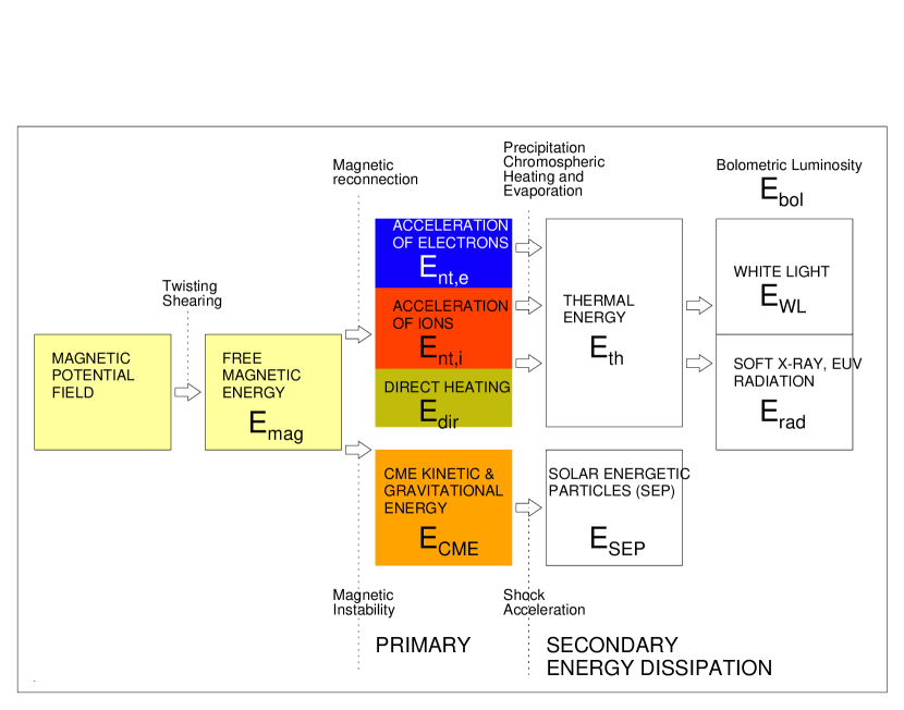
Figure 1: Schematic diagram of energy input (free magnetic energy $E_{\mathrm{mag}}$), primary energy dissipation processes (electron acceleration $E_{\mathrm{nt,e}}$, ion acceleration $E_{\mathrm{nt,i}}$, direct heating $E_{\mathrm{dir}}$, and launching of CME $E_{\mathrm{CME}}$), and secondary energy dissipation processes (thermal energy $E_{\mathrm{th}}$, solar energetic particles $E_{\mathrm{SEP}}$, and bolometric luminosity $E_{\mathrm{bol}}$, with radiative energies observed in white-light $E_{WL}$, soft X-rays and EUV $E_{\mathrm{rad}}$).

The energy flow in solar flares and CMEs passes through several processes which are depicted in the diagram of Fig. 1. Initially, a stable non-flaring active region exists with a near-potential magnetic field with energy $E_{p}$, which then becomes twisted and sheared, building up nonpotential energy $E_{\mathrm{np}}$ and the free energy, $E_{\mathrm{free}}=E_{\mathrm{np}}-E_{p}$, of which a fraction $E_{\mathrm{mag}}\leq E_{\mathrm{free}}$ is dissipated during a flare (e.g., Schrijver et al. 2008; Aschwanden 2013). There are three primary energy dissipation processes that follow after a magnetic instability, typically a magnetic reconnection process, spawning (1) the acceleration of nonthermal particles (e.g., reviews by Miller et al. 1997; Aschwanden 2002; Benz 2008; Holman et al. 2011), with electron energy $E_{\mathrm{nt,e}}$ and ion energy $E_{\mathrm{nt,i}}$, providing (2) direct heating in the magnetic reconnection region, $E_{\mathrm{dir}}$ (e.g., Sui and Holman 2003; Caspi and Lin 2010; Caspi et al. 2015), and are often accompanied by (3) an eruptive process, which can be a complete eruption of a CME or filament, or a semi-eruptive energy release, also known as “failed eruption”, in the case of a confined flare (e.g., Török and Kliem 2005). The CME process carries an energy of $E_{\mathrm{CME}}=E_{\mathrm{kin}}+E_{\mathrm{grav}}$, consisting of the kinetic energy $E_{\mathrm{kin}}$ and the gravitational potential energy $E_{\mathrm{grav}}$, to lift a CME from the solar surface into the heliosphere. These primary energy dissipation processes allow us to test the primary energy closure equation,

$$E_{\mathrm{mag}}=(E_{\mathrm{nt}}+E_{\mathrm{dir}}+E_{\mathrm{CME}})=(E_{\mathrm{nt,e}}+E_{\mathrm{nt,i}}+E_{\mathrm{dir}}+E_{\mathrm{CME,kin}}+E_{\mathrm{CME,grav}})\ ,$$ (1)

where the left-most side of the equation contains the total (magnetic) energy input (or storage), and the right-most side of the equation contains the total energy output (or dissipation).

After this primary step in the initiation of a flare and CME, secondary energy dissipation processes kick in. Nonthermal particles are accelerated along bi-directional trajectories that lead out of the magnetic reconnection region, where most particles precipitate down to the chromosphere, heat chromospheric plasma and drive evaporation of the heated plasma up into the corona (e.g., Antonucci and Dennis 1983), while other particles escape into interplanetary space (see reviews by Hudson and Ryan 1995; Aschwanden 2002; Lin 2007). The flare arcade that becomes filled with heated chromospheric plasma radiates and loses its energy by conduction and radiation in soft X-rays (SXR) and extreme ultra violet (EUV). The thermal energy content $E_{\mathrm{th}}$ can be calculated from the total emission measure observed in SXR and EUV and should not exceed the nonthermal energy, $E_{\mathrm{nt}}=E_{\mathrm{nt,e}}+E_{\mathrm{nt,i}}$, unless there are other heating processes besides the electron beam-driven heating observed in hard X-rays (according to the thick-target bremsstrahlung model of Brown 1971). Thus we can test the following energy inequality between thermal and nonthermal energies (if we neglect direct heating),

$$E_{\mathrm{th}}\leq E_{\mathrm{nt}}=(E_{\mathrm{nt,e}}+E_{\mathrm{nt,i}})\ .$$ (2)

Radiation is not only produced at SXR and EUV wavelengths ($E_{\mathrm{th}}$), but also in visible and near-ultraviolet wavelengths, recorded as white-light flare emission, being the largest contributor to the bolometric energy or luminosity $E_{\mathrm{bol}}$, which contains vastly more radiative energy than observed in SXR (Woods et al. 2004, 2006; Kretzschmar 2011). Using a superimposed epoch analysis of 2100 C-, M-, and X- class flares, Kretzschmar (2010; 2011 and Table 1 therein) calculated the total solar irradiance (TSI) for five synthesized flare time profiles. The so determined continuum emission produced by white-light flares allows us to compare another pair of energies, which relates the total thermal energy $E_{\mathrm{th}}$ to the bolometric luminosity, produced by the flare impact of precipitating particles, radiative back-warming, and locally enhanced ionization, enhancing bound-free and free continuum emission (e.g., Najita and Orrall 1970; Hudson 1972; Ding et al. 2003; Battaglia and Kontar 2011; Battaglia et al. 2011; Xu et al. 2014),

$$E_{\mathrm{bol}}\approx E_{\mathrm{th}}\ .$$ (3)

Another secondary process is the acceleration of nonthermal particles by the CME, which is produced by shock acceleration in very fast CMEs, observed in form of solar energetic particle (SEP) events (e.g., see review by Reames 2013), which allows us to test another energy inequality,

$$E_{\mathrm{SEP}}\leq E_{\mathrm{CME}}=E_{\mathrm{CME,kin}}+E_{\mathrm{CME,grav}}\ .$$ (4)

The energy closure studied here depends, of course, on specific physical models of flares and CMEs. Here we discuss only the most common solar flare models, but we have to make a disclaimer that alternative flare models may deviate from the energy closure relationships and inequalities discussed here. Another important issue in any energy closure relationship concerns the double-counting of energies if there are multiple energy conversion processes acting at the same time or near-simultaneously. We attempt to distinguish between primary and secondary energy dissipation mechanisms, as shown in Fig. 1.

The aim of this paper is to summarize the assumptions that went into the derivation of the various measured and observationally derived energy parameters (Section 2), to test energy closure (Section 3), to discuss some physical processes that play a role in the energy closure relationships (Section 4), and final conclusions (5).

2 FLARE AND CME ENERGIES

In order to characterize the different forms of energies that can be measured or derived in solar flares and CMEs we start with a brief description of the basic assumptions that are made in the four relevant studies (Papers I, II, III, IV, and references therein) in the derivation of various forms of energies.

We will quote the mean ratios of the various energy conversion processes $E_{x}$ to the dissipated magnetic energy $E_{\mathrm{mag}}$, by averaging their logarithmic values, so that the logarithmic standard deviation $\sigma_{log}$ corresponds to a factor with respect to the mean value. For instance, the ratio of the nonthermal energy to the magnetically dissipated energy (Section 2.2) has a logarithmic mean and standard deviation of ${}^{10}log(q_{nt,e})={}^{10}log{(E_{nt,e}/E_{\mathrm{mag}})}=-0.39\pm 0.89$, which we quote as a linear value with a standard deviation factor, i.e., $q_{nt,e}=(E_{nt,e}/E_{\mathrm{mag}})=10^{-0.39}\div 10^{0.89}=0.41\div 7.7$. Thus the range of one standard deviation, i.e., $[0.41/7.7,0.41\times 7.7]=[0.05,3.2]$, includes 68% of the events. The statistical error $e_{x}$ of the mean value $q_{x}$ is then obtained by dividing the standard deviation by the square root of $n_{x}$ events. For instance, the error $e_{x}$ of the mean nonthermal energy based on $n=76$ values is $e_{nt,e}=10^{0.89/\sqrt{76}}-1=0.26$, given as $q_{x}\pm e_{x}=0.41\pm 0.26$, which expresses the 68% statistical probability to find a mean value in this range for another data set with the same number of $n=76$ events.

2.1 Magnetic Energies

The basic assumptions in the calculation of magnetic energies are (Paper I): (1) The coronal magnetic field in a flaring active region is nonpotential and has a nonpotential energy $E_{\mathrm{np}}=E_{p}+E_{\mathrm{free}}$, with the free energy being larger than zero; (2) The free energy $E_{\mathrm{free}}=B_{\varphi}^{2}/8\pi$ can largely be represented by helically twisted fields ${\bf B}={\bf B}_{r}+{\bf B}_{\varphi}$. It is composed of a potential field component ${\bf B}_{r}$ and a nonpotential field component ${\bf B}_{\varphi}$ in perpendicular (azimuthal) direction to the potential field, which is induced by vertical currents ${\bf j}(4\pi/c)=(\nabla\times{\bf B})$ above magnetic field concentrations (such as sunspots or in active region plages); (3) The line-of-sight component $B_{z}(x,y)$ can be measured from magnetograms (such as the Helioseismic and Magnetic Imager (HMI); (4) The photospheric magnetic field is not force-free and the transverse magnetic field components cannot be directly measured from photospheric magnetograms, such as with tradidional nonlinear force-free field (NLFFF) codes (Aschwanden 2016b); (5) Coronal loops are embedded in low plasma-$\beta$ regions and are force-free before and after a flare or CME launch; (6) The transverse components $B_{x}(x,y)$ and $B_{y}(x,y)$ can be constrained from the 2D directional vectors of coronal loops observed in EUV wavelengths (such as with the Atmospheric Imaging Assembly (AIA), using an automated loop tracing algorithm; (7) A flare or launch of a CME dissipates a fraction of the free magnetic energy, and thus the time evolution of the free energy $E_{\mathrm{free}}(t)$ exhibits in principle a step function from a higher (preflare) to a lower (postflare) value of the free energy; (8) The evolution of the free energy $E_{\mathrm{free}}(t)$ may exhibit an apparent increase due to coronal illumination effects (such as chromospheric evaporation) at the beginning of the impulsive flare phase, before the decrease of free energy is observed.

In our global energetics study on magnetic energies (Paper I) we included all Geostationary Operational Environmental Satellite (GOES) X- and M-class flares during the first 3.5 years of the Solar Dynamics Observatory (SDO) mission, which amounted to a total data set of 399 flare events. Restricting the magnetic analysis to events with a longitude difference of $|l-l_{0}|\leq 45^{0}$ from the central meridian ($l_{0}$) due to foreshortening effects in the magnetograms, we were able to determine the flare-dissipated magnetic energy in 172 events, covering a range of $E_{\mathrm{mag}}=(1.5-1500)\times 10^{30}$ erg. The dissipated flare energy $E_{\mathrm{mag}}$ is highly correlated with the free energy $E_{\mathrm{free}}$, the potential energy $E_{p}$, and the nonpotential energy $E_{\mathrm{np}}$ (see Fig. 13 in Paper I).

In a previous study on the global flare energetics (Emslie et al. 2012), no attempt was made to calculate a nonpotential magnetic field energy change during flares, but instead an ad hoc value of 30% of the potential energy was assumed. The inferred range of $E_{\mathrm{mag}}=(110-2900)\times 10^{30}$ erg appears to over-estimate the dissipated magnetic flare energy by one to two orders of magnitude for M-class flares, when compared with our study.

2.2 Nonthermal Electron Energies

The nonthermal energies, which includes the kinetic energy of particles accelerated out of the thermal population, are derived from hard X-ray spectra observed with the Ramaty High-Energy Solar Spectroscopic Imager (RHESSI) instrument (Paper III). The basic assumptions are: (1) Particle acceleration occurs in magnetic reconnection processes, either by electric fields, by stochastic wave-particle interactions in turbulent plasmas, or by shock waves; (2) Hard X-ray spectra are produced by bremsstrahlung (free-free and free-bound emission) of both thermal and nonthermal particles; (3) The thermal and nonthermal emission can be distinguished in hard X-ray spectra by an exponential-like spectrum at low energies (typically 6-20 keV) and a powerlaw-like spectrum at higher energies (typically 20-50 keV); (4) The energy in nonthermal electrons can be calculated by spectral integration of the powerlaw-like nonthermal spectrum (with a slope $\delta$) above some low-energy cutoff $e_{c}$; (5) The low-energy cutoff $e_{c}$ can be estimated from the warm-target model of Kontar et al. (2015) according to $e_{c}=\delta k_{B}T_{e}$, where $T_{e}$ is the average temperature of the warm-target, in which the electrons diffuse before they lose their energy by collisions, and $\delta$ is the power law slope of the nonthermal electron flux; (6) The warm-target temperature $T_{e}$ can be estimated from the mean value of the peak temperature of the differential emission measure (DEM) distribution observed with AIA in the temperature range of $T_{e}\approx 0.5-20$ MK, which was found to be $T_{e}=8.6$ MK in the statistical average of all events. A mean value of the low-energy cutoff $e_{c}=6.2\pm 1.6$ keV was obtained from the entire ensemble of analyzed events (see discussion in Section 4.1).

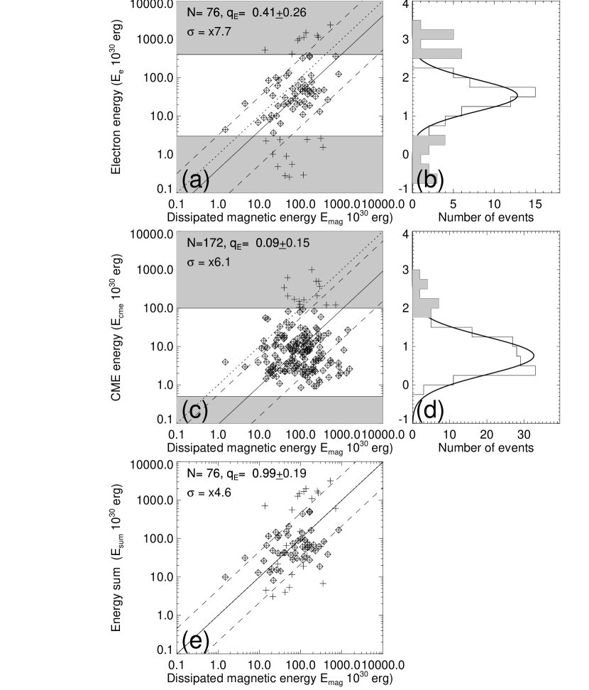
Figure 2: Cross-correlation plots of the electron energy $E_{\mathrm{nt,e}}$ (a), the CME energy $E_{\mathrm{CME}}$ (c), and the energy sum $E_{\mathrm{sum}}=E_{\mathrm{nt,e}}+E_{\mathrm{nt,i}}+E_{\mathrm{dir}}+E_{\mathrm{CME}}$ with the dissipated magnetic energy $E_{\mathrm{mag}}$ (e). Log-normal Gaussian distributions are fitted (b,d) to the histogrammed events and the outlier data points are marked with crosses and the ranges are shown with grey areas in (a,b,c,d). Normal data points without outliers are marked with diamonds. The mean (logarithmic) ratios are indicated with a diagonal solid line, the standard deviations with dashed lines, and equivalence with dotted lines. The parameters listed in each panel include the number of events $N$, the (logarithmic) mean energy ratio $q_{E}$, and the standard deviation factor $\sigma$, as defined at the beginning of Section 2.

In our global energetics study on nonthermal energies (Paper III) we analyzed RHESSI spectra in 191 M- and X-class flare events, amounting to 48% of the total data set, while the remainder was missed due to the duty cycle of RHESSI in the day/night portions of the spacecraft orbit. The nonthermal energies of the 191 analyzed events covers a range of $E_{\mathrm{nt,e}}=(0.05-8000)\times 10^{30}$ erg. Cross-correlating the nonthermal energy in electrons $E_{\mathrm{nt,e}}$ with the dissipated magnetic energy $E_{\mathrm{mag}}$, we find an overlapping subset of 76 events, which exhibits a mean (logarithmic) energy ratio of $E_{\mathrm{nt,e}}/E_{\mathrm{mag}}=0.41\pm 0.26$, with a standard deviation factor of $\sigma=7.7$ (Fig. 2a). The distribution of (logarithmic) electron energies can be represented by a log-normal (Gaussian) distribution (Fig. 2b) that extends over a range of $E_{\mathrm{mag}}=(3-400)\times 10^{30}$ erg. Outliers are likely to be caused due to small errors in the estimate of the warm-target temperature and the related low-energy cutoff, which are hugely amplified in the resulting nonthermal energies. If we remove the outliers (in excess of $\lower 1.72218pt\hbox{$\;\buildrel>\over{\scriptstyle\sim}\;$}3$ standard deviations in the tails of the Gaussian distribution in Fig. 2b), we obtain 55 events with a ratio of

$$E_{\mathrm{nt,e}}/E_{\mathrm{mag}}=0.51\pm 0.17\ ,$$ (5)

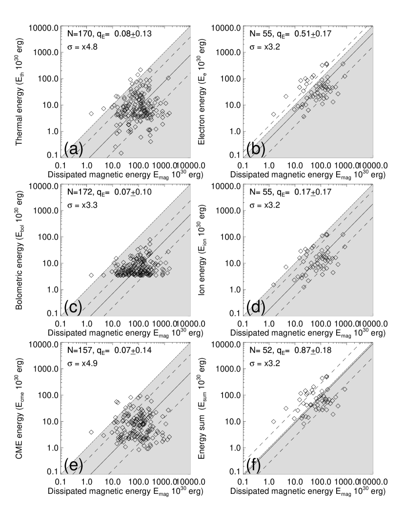
Figure 3: Cross-correlation plots of the thermal energy $E_{\mathrm{th}}$ (a), the bolometric energy $E_{\mathrm{bol}}$ (c), the CME energy $E_{\mathrm{CME}}$ (e), the nonthermal electron energy $E_{\mathrm{nt,e}}$ (b), the nonthermal ion energy $E_{\mathrm{nt,i}}$ (c), and the energy sum $E_{\mathrm{sum}}=E_{\mathrm{nt,e}}+E_{\mathrm{nt,i}}+E_{\mathrm{dir}}+E_{\mathrm{CME}}$ (f), with the dissipated magnetic energy $E_{\mathrm{mag}}$. Outlier events (marked with cross symbols in Fig. 2) have been removed in this selection of datapoints. The mean (logarithmic) ratios are indicated with a diagonal solid line, the standard deviations with dashed lines, and equivalence with dotted diagonal line bordering the grey area.

with a much smaller standard deviation factor of $\sigma=3.2$ as shown in Fig. 3b.

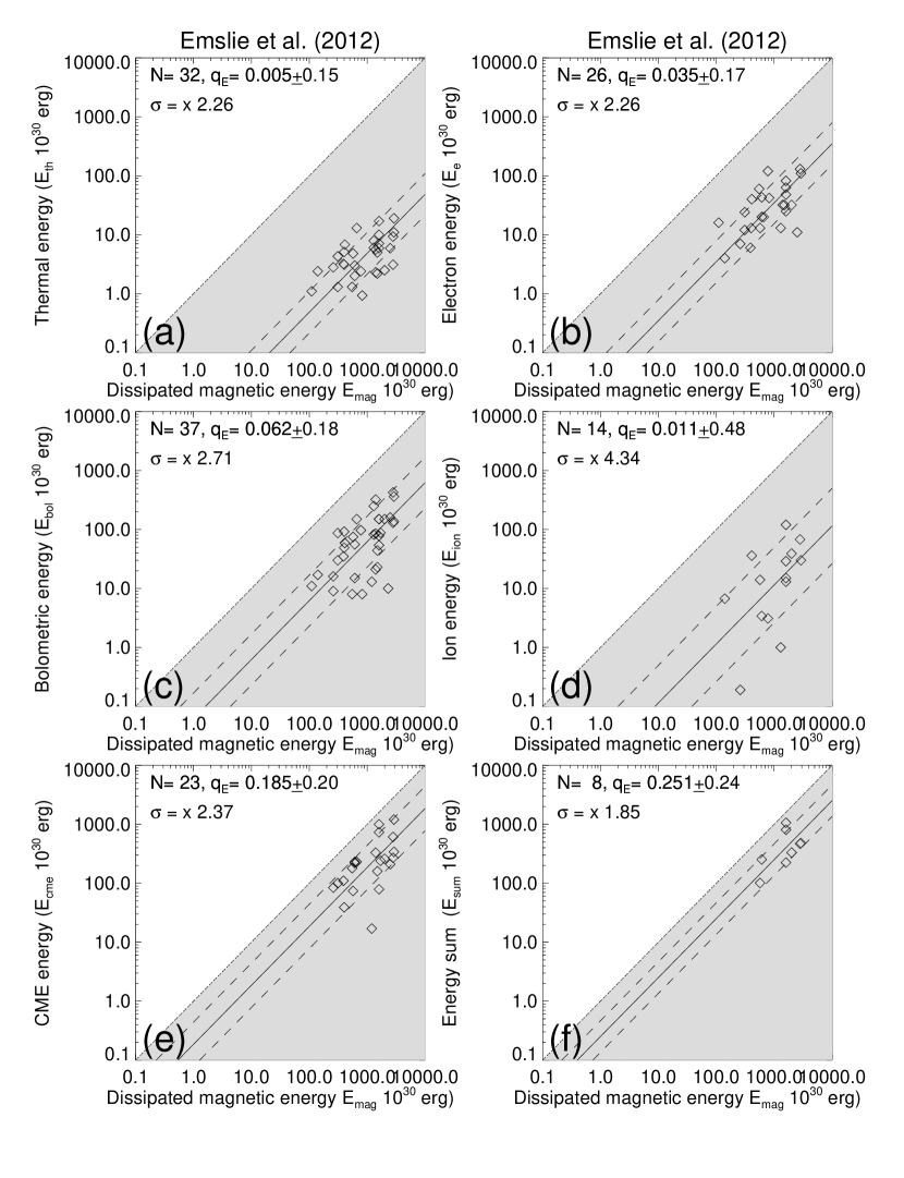
Figure 4: Cross-correlation plots of the same parameters as shown in Fig. 3, but for the data set of 37 eruptive flare events analyzed in Emslie et al. (2012).

In the previous study on the global flare energetics by Emslie et al. (2012), RHESSI data have been used also, but the warm-target model did not exist yet, since it was derived later (Kontar et al. 2015), but is currently considered to be the best physical model for estimating a lower limit of the low-energy cutoff of nonthermal electrons (Paper III). For the temperature in the warm-target model we used for all events the same mean value of $T_{e}=8.6$ MK, which was obtained from the emission measure weighted DEMs, averaged during the entire flare durations, and averaged from all analyzed flare events. In comparison, the low-energy cutoff value $e_{c}\approx 20$ keV of Emslie et al. (2012), based on the largest value that still gave an acceptable fit (reduced $\chi^{2}\approx 1$), represents an upper limit, while our value of $e_{c}\approx 6$ keV appears to be rather a lower limit. The resulting mean energy ratio of the nonthermal electron energy to the dissipated magnetic energy was found to be $E_{\mathrm{nt,e}}/E_{\mathrm{mag}}=0.03\pm 0.02$ in Emslie et al. (2012) with a standard deviation factor of $\sigma=2.3$ for 26 events (Fig. 4b). Thus the efficiency of particle acceleration was found to be substantially lower in Emslie et al. (2012), by a factor of $\approx 16$, compared with our value of $E_{\mathrm{nt,e}}/E_{\mathrm{mag}}=0.51\pm 0.17$ (Fig. 3b). This discrepancy appears to be the consequence of two effects, the over-estimate of magnetic energies, and the adoption of upper limits for the low-energy cutoff.

2.3 Nonthermal Ion Energies

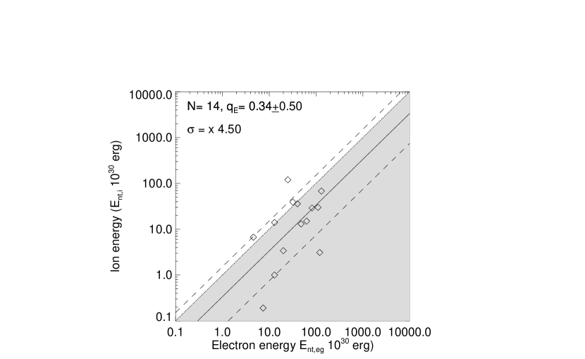
Figure 5: Cross-correlation between nonthermal ion energies $E_{\mathrm{nt,i}}$ versus the nonthermal electron energies $E_{\mathrm{nt,e}}$ from a dataset of 37 eruptive flare events analyzed in Emslie et al. (2012).

In the absence of suitable RHESSI gamma-ray data analysis we resort to the statistics of the earlier study by Emslie et al. (2012), which yields the ratios of ion energies to electron energies in 14 eruptive flare events, which we show in Fig. 5 (see also Table 1 and Fig. 2 in Emslie et al. 2012). The mean (logarithmic) ratio is found to be,

$$E_{\mathrm{nt,i}}/E_{\mathrm{nt,e}}=(0.34\pm 0.50)\ ,$$ (6)

where the standard deviation factor is $\sigma=4.5$. Thus ions carry about a third of the energy in accelerated electrons (above a low-energy cutoff constrained by acceptable fits). These flare-accelerated ion energies are based on RHESSI measurements of the fluence in the 2.223 MeV neutron-capture gamma-ray line (Shih 2009; Shih et al. 2009). A caveat has to be added that the ion energies calculated in Emslie et al. (2012) used a low-energy cutoff of $\lower 1.72218pt\hbox{$\;\buildrel>\over{\scriptstyle\sim}\;$}1$ MeV, and thus may represent lower limits on the ion energies and the related ion energy ratios.

The application of the ion/electron energy ratio (Eq. 6) to the nonthermal electron energies analyzed in our data yields a mean (logarithmically averaged) ratio of (Fig. 3d)

$$E_{\mathrm{nt,i}}/E_{\mathrm{mag}}=(0.17\pm 0.17)\ ,$$ (7)

which implies that about a sixth of the total dissipated magnetic energy is converted into acceleration of ions (with energies of $\lower 1.72218pt\hbox{$\;\buildrel>\over{\scriptstyle\sim}\;$}1$ MeV), while about half of the total magnetic energy (Eq. 5) goes into acceleration of electrons (above the mentioned low-energy cutoff of $e_{c}\lower 1.72218pt\hbox{$\;\buildrel>\over{\scriptstyle\sim}\;$}6$ keV).

2.4 Thermal Energies

The thermal energy in flares is mostly due to a secondary energy conversion process and has been quantified in Paper II. The basic assumptions in the derivation of thermal energies are: (1) Solar flares have a multi-thermal energy distribution; (2) The multi-thermal energy can be calculated from the temperature integral of the DEM distribution and a volume estimate at the peak time of the flare; (3) AIA data in all 6 coronal wavelengths provide a DEM in the temperature range of $T_{e}\approx 0.5-20$ MK (Boerner et al. 2014), while RHESSI is sensitive to the high-temperature tail of the DEM at $T_{e}\approx 20-40$ MK (Caspi 2010; Caspi and Lin 2010; Caspi et al. 2014, 2015; Ryan et al. 2014); (4) A suitably accurate DEM method is the spatial synthesis method (Aschwanden et al. 2013, 2015b), which fits a Gaussian DEM in each spatial (macro)pixel of AIA images in all coronal wavelengths and synthesizes the DEM distribution by summing the partial DEMs over all (macro)pixels; (5) The flare volume can be estimated from the geometric relationship $V\approx A^{3/2}$, where the flare area $A$ is measured above some suitable threshold in the emission measure per (macro)pixel (assuming a filling factor of unity for sub-pixel features); (6) The thermal energy content dominates at the flare peak, while conductive and radiative losses as well as secondary heating episodes (indicated by subpeaks in the SXR and EUV flux) are neglected in our analysis. The thermal energy derived here thus represents a lower limit. Note that the thermal energy is calculated at the flare peak time (when the peak value of the total emission measure is reached), and thus represents the peak thermal energy, while non-thermal energies in electrons (Section 2.2) are calculated by time integration over the entire flare duration.

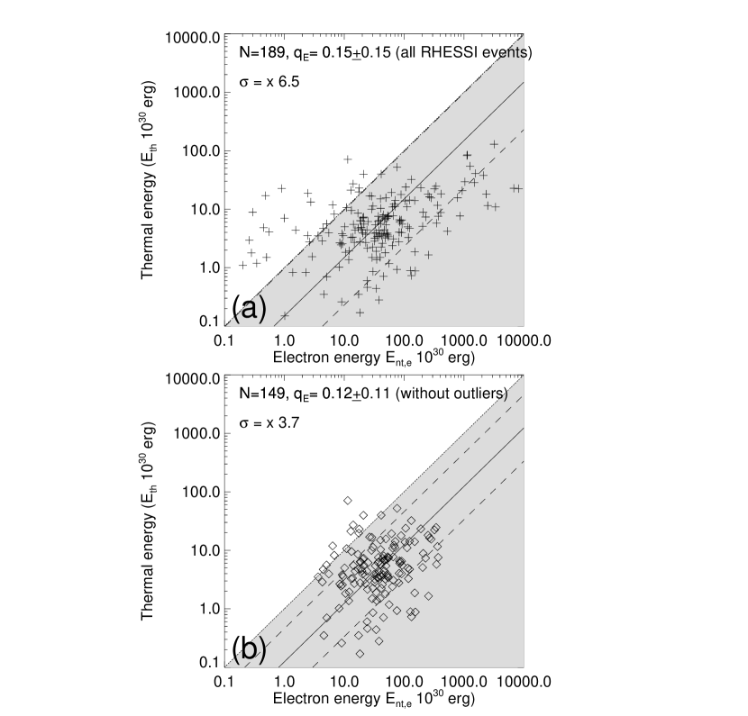
Figure 6: Cross-correlation between thermal energies $E_{\mathrm{th}}$ and nonthermal electron energies $E_{\mathrm{nt,e}}$, for all RHESSI events (top panel), and for a subset without outliers (bottom panel) according to Fig. 2b. Note that the thermal energy generally does not exceed the nonthermal energy (equivalence is indicated with a diagonal bordering the grey zone).

In our previous global energetics study on thermal energies (Paper II) we were able to derive the thermal energy in 391 flare events (of GOES M- and X-class), and find an energy range of $E_{\mathrm{th}}=(0.15-215)\times 10^{30}$ erg. If we want to compare these thermal energies with nonthermal energies, the sample reduces to 189 events, yielding a mean (logarithmic) ratio of $E_{\mathrm{th}}/E_{\mathrm{nt,e}}=(0.15\pm 0.15)$, with a standard deviation factor of $\sigma=6.5$ (Fig. 6a). Removing the outliers by restricting the valid energy range to $E_{\mathrm{nt,e}}=(3-400)\times 10^{30}$ erg (see Fig. 2b), we obtain a somewhat more accurate value for 149 events (Fig. 6b),

$$E_{\mathrm{th}}/E_{\mathrm{nt,e}}=(0.12\pm 0.11)\ .$$ (8)

This means that only 12% of the nonthermal energy in electrons is converted into heating of the flare plasma, which appears to be a low value for the (warm) thick-target bremsstrahlung model. Alternative studies find that thermal and nonthermal energies are of the same magnitude (Saint-Hilaire and Benz 2005; Warmuth and Mann 2016a,b). However, since we neglected conductive and radiative losses as well as multiple heating episodes (besides the flare peak), the thermal energy may be grossly underestimated. In addition, the nonthermal energy in electrons may be over-estimated due to the lower limit of the low-energy cutoff $e_{c}\approx 6$ keV. However, since electron beam-driven chromospheric plasma heating is a secondary energy dissipation process, it does not affect the energy closure relationship (Eq. 1) of primary energy dissipation processes.

Comparing the thermal energy with the available magnetic energy we consequently find a relatively low value of (Fig. 3a) for 170 events,

$$E_{\mathrm{th}}/E_{\mathrm{mag}}=(0.08\pm 0.13)\ .$$ (9)

The previous study by Emslie et al. (2012) finds an even lower value of $E_{\mathrm{th}}=(0.005\pm 0.15)\ E_{\mathrm{mag}}$ (Fig. 4a), which is mostly caused by the use of an iso-thermal definition of the thermal energy. A multi-thermal definition would yield a factor of 14 higher values for the thermal energy (Paper II). Moreover, no high-resolution imaging data in SXR and EUV were available in the study of Emslie et al. (2012). Even now, SXR images are available from EIS/Hinode occasionally only, but were not used in this study.

Besides electron-beam heating of the chromosperic thick target, non-beam heating or direct heating may also play a role (e.g., Sui and Holman 2003; Caspi and Lin 2010; Caspi et al. 2015). We derive lower limits for the energy of direct heating processes for those flares where the thermal energy exceeds the nonthermal energy in electrons and ions (see Fig. 1), which yields a lower limit of

$$E_{\mathrm{dir}}/E_{\mathrm{mag}}=(E_{\mathrm{th}}-E_{\mathrm{nt,e}}-E_{\mathrm{nt,i}})/E_{\mathrm{mag}}=(0.07\pm 0.17)\ .$$ (10)

2.5 Radiated Energy from Hot Flare Plasma

In this section we examine the thermally radiated energy over all wavelengths from the hot ($>$4 MK) coronal flare plasma. We determined these energies from tables of the radiative loss rate as a function of emission measure and temperature generated using the CHIANTI atomic physics database (Dere et al. 1997; Del Zanna et al. 2015) and the methods of Cox and Tucker (1969). The temperatures and emission measures were calculated using the ratio of the GOES/XRS 0.5–4 Å to 1–8 Å channels (Thomas et al. 1985; White et al. 2005). As part of these calculations, coronal abundances (Feldman et al. 1992), ionization equilibria (Mazzotta et al. 1998), and a constant density (10¹⁰ cm^-3) were assumed. In addition, this methodology implicitly assumes that the plasma is isothermal, although this is not the case for the flares analyzed here and in general (Aschwanden et al. 2015). The isothermal assumption is therefore an important caveat here, but is consistent with previous energetics studies (Emslie et al. 2015). To ensure reliable results, the flare emission in both GOES/XRS channels was separated from the background using the Temperature and Emission measure-Based Background Subtraction algorithm (TEBBS; Ryan et al. 2012), before the temperatures and emission measures were calculated.

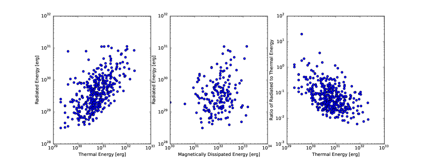
Figure 7: Thermally radiated energies from the hot ($>$4 MK) coronal plasma as a function of thermal and magnetically dissipated energies: (a) Radiated energy versus thermal energy; (b) Radiated energy versus magnetically dissipated energies; and (c) Ratio of radiated to thermal energies versus thermal energy.

Fig. 7a shows the coronal thermally radiated energy as a function of thermal energy for 389 of the 399 flares considered in this study. There is a correlation between flare thermal energy and radiative losses from the hot coronal plasma, as expected. The (logarithmic) average ratio of radiated losses to thermal energy was found to be

$$E_{rad}/E_{th}=0.07\pm 0.06$$ (11)

This consistent with Emslie et al. (2012) who found $E_{rad}/E_{th}=0.17\pm 0.15$. Fig. 7b compares the thermally radiated coronal losses to the total magnetic dissipated energy for the 171 flares common to this study and Aschwanden et al. (2014). The average ratio was found to be

$$E_{rad}/E_{mag}=0.004\pm 0.13$$ (12)

From the above results it is clear that thermally radiated energy from the hot coronal plasma dissipates only a small fraction of the thermal and magnetically dissipated energies in a flare.

Although there is a positive correlation between the thermal and radiated energies, there is a reciprocal relationship in the ratio of radiated to thermal energy, as shown in Fig. 7c. This implies flares with larger thermal energy dissipate a smaller fraction of that energy via thermal radiation. This is qualitatively consistent with simple hydrodynamic flare cooling models that predict that radiative losses and conductive losses are anti-correlated at higher plasma temperatures (e.g., Cargill et al. 1995). No such relationship is evident from the results of Emslie et al. (2012) because of their small sample size (38 events).

2.6 Bolometric Energies

In the largest flares, white-light emission from deep in the chromosphere can be observed, supposedly caused by precipitation of nonthermal electrons and ions into the deeper chromospheric layers (Hudson 1972). Hudson finds that the $\lower 1.72218pt\hbox{$\;\buildrel>\over{\scriptstyle\sim}\;$}5$ keV electrons in major flares have sufficient energy to create long-lived excess ionization in the heated chromosphere to enhance free-free and free-bound continuum emission, visible in broadened hydrogen Balmer and Paschen lines. Energization to lower altitudes down to the photosphere can also be accomplished by photo-ionization, a mechanism termed radiative backwarming (Hudson 1972).

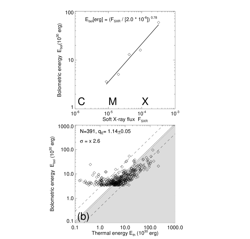
Figure 8: Cross-correlation between bolometric energy $E_{\mathrm{bol}}$ and the SXR flux $F_{\mathrm{SXR}}$ of the GOES 1-8 Å flux according to Kretzschmar (2011) (top panel). The resulting correlation between the bolometric energy $E_{\mathrm{bol}}$ and the thermal energy $E_{\mathrm{th}}$ yields a mean ratio of almost unity.

Kretzschmar (2011) recently demonstrated that white-light continuum is the major contributor to the total radiated energy in most flares, where the continuum is consistent with a blackbody spectrum at $\approx 9000$ K. From a set of 2100 superimposed C- to X-class flares, Kretzschmar (2011; Table 1) calculated the total solar irradiance (TSI), which can be characterized by a scaling law relationship between the bolometric energy $E_{\mathrm{bol}}$ (in erg) and the GOES 1-8 Å SXR flux $F_{\mathrm{SXR}}$ in units of W m^-2 (Fig. 8a; top panel),

$${E_{\mathrm{bol}}\over 10^{30}\ {\rm[erg]}}\approx\left({F_{\mathrm{SXR}}\over 2.0\times 10^{-6}\ {\rm W}\ {\rm m}^{-2}}\right)^{0.78}\ .$$ (13)

If we apply this empirical scaling law to the GOES fluxes and thermal energy $E_{\mathrm{th}}$ from AIA data analyzed in Paper II, we obtain an energy ratio $E_{\mathrm{bol}}/E_{\mathrm{th}}$ of almost unity (Fig. 8b),

$$E_{\mathrm{bol}}/E_{\mathrm{th}}=(1.14\pm 0.05)\ ,$$ (14)

and thus the bolometric energy matches almost the thermal energy contained in the coronal flare plasma observed in SXR and EUV. The total flare irradiance was found to exceed SXR emission by far. Woods et al. (2004) report that 19% of the total emission comes from the XUV range (0-27 nm), which implies that SXR emission amounts to less than a fifth of the total emission. Both Woods et al. (2006) and Kretzschmar (2011) report that only 1% of the total bolometric luminosity is radiated in the GOES SXR range (1-8 A). Since both the bolometric and the thermal energy are secondary or tertiary energy conversions in the flare process (Fig. 1), they do not matter to the primary energy closure (Eq. 1) investigated here, but allow us to set limits on each energy conversion process.

2.7 CME Energies

Almost all large flares are accompanied by a CME, and even most mid-sized flares are associated with a CME, down to the GOES C-class level (Andrews 2003). The total energy of a CME can be calculated either from the white-light polarized brightness in coronagraph images, or from the EUV dimming in the CME footpoint area. We used the second method to calculate a statistical sample of CME energies using AIA data (Paper IV). The main assumptions in our analysis are: (1) A flare-associated dimming of the total emission measure observed in EUV and SXR indicates a mass loss in the flare area, which constitutes the existence of a CME event (Aschwanden et al. 2009; Mason et al. 2014, 2016); (2) The DEM obtained from AIA in the temperature range of $T_{e}\approx 0.5-20$ MK largely rules out that the observed dimming is a temperature (heating or cooling) effect, because the particle number in a CME is approximately conserved when a DEM is integrated over the full coronal temperature range; (3) The EUV dimming profile is expected to drop from a higher preflare level after the CME starts in the impulsive flare phase, but an initial compression (or implosion) process can produce an initial increase in the EUV total emission measure before the EUV dimming sets in; (4) The spatial synthesis method (Aschwanden et al. 2013), which fits a Gaussian DEM in each spatial (macro)pixel of AIA images in all coronal wavelengths and synthesizes the DEM distribution by summing the partial DEMs over all (macro)pixels, provides a suitable method to calculate the evolution of the total emission measure; (5) The temporal evolution of a CME in the EUV dimming phase can be modeled with a radial adiabatic expansion process, which accelerates the CME and produces a rarefaction of the density inside the CME leading edge envelope; (6) The volume of a CME can be quantified by the footpoint or EUV dimming area and the vertical density scale height of a hydrostatically stratified corona initially, and with a reciprocal relationship between the density and volume during the subsequent adiabatic expansion phase. (7) The total energy of a CMEs consists of the kinetic energy and the gravitational potential energy to lift a CME from the solar surface to infinity. The pressure in CMEs is modeled with adiabatic expansion models, and thus neglects temperature changes during the initial expansion phase of the CME (Paper IV); (8) A subset of non-eruptive flares, called confined flares, does not produce a CME, in which case our calculation of a CME energy corresponds to the energy that goes into the adiabatic expansion up to a finite altitude limit where the eruption stalls.

In our previous global energetics study on CME energies (Paper IV) we were able to derive the CME energy in all 399 flare events (of GOES M- and X-class), and find an energy range of $E_{\mathrm{CME}}=(0.25-1000)\times 10^{30}$ erg. Removing a few outliers with the highest energies that show an excess of $\lower 1.72218pt\hbox{$\;\buildrel>\over{\scriptstyle\sim}\;$}2$ standard deviations in the upper tail of a statistical random distribution (Fig. 2d), we obtain an improved valid range of $E_{\mathrm{CME}}=(0.25-100)\times 10^{30}$ erg for the remaining 386 events (or 97% of the entire data set).

Comparing the CME energies with those events where the magnetic energy could be calculated, we find 157 events with a mean (logarithmic) energy ratio of (Fig. 3e),

$$E_{\mathrm{CME}}/E_{\mathrm{mag}}=(0.07\pm 0.14)\ .$$ (15)

In complex CME events with multiple convolved EUV dimming phases, in particular for SEP events (Table 1), the CME speed, and thus the kinetic CME energy is likely to be substantially underestimated with the EUV dimming method, in which case (Fig. 3e) we substitute the AIA-inferred CME values with the Large Angle and Spectrometric Coronagraph Experiment (LASCO)-inferred white-light values (whenever the LASCO CME energy is larger than the AIA CME energy). The AIA CME energies are shown in Fig. 3e, and their comparison with LASCO CME energies is shown in Fig. 18 of Paper IV. The LASCO CME energies were found to be larger than the AIA values in 42%. On the other hand, LASCO underestimates the CME energy also, in particular for halo CMEs, because the occulted material is missing and because the projected speed is a lower limit to the true 3-D speed. In other words, both the LASCO and the AIA method provide lower limits of CME energies, which is the reason why we use the higher value of the two lower limits as the best estimate of CME energies here (Fig. 3e). Therefore, less energy goes into the creation of a CMEs (Eq. 15) than what goes into the acceleration of nonthermal particles (Eq. 5).

The previous study by Emslie et al. (2012) finds about a factor of two higher mean value of $E_{\mathrm{CME}}/E_{\mathrm{mag}}=(0.19\pm 0.20)$ (Fig. 4e). The main reason for this difference in the CME energy is that LASCO data (used in Emslie et al. 2012) yield a systematically higher leading-edge velocity than the bulk plasma velocity determined with AIA (used here mostly), which enters the CME kinetic energy with a nonlinear (square) dependence. Another reason is that the convolution bias in complex events tends to produce lower limits of CME speeds (Paper IV, Section 3.1).

2.8 SEP Energies

It is generally believed that at least two processes accelerate particles in the solar flare and associated CME eruptions. First, as discussed above, magnetic reconnection processes in solar flares release energy that rapidly accelerates ions and electrons, most of which interact in the solar atmosphere to produce X-rays, gamma rays, and longer-wavelength radiation. Some fraction of these “flare-accelerated” particles can also escape into the interplanetary medium, where they can be identified by their composition (e.g., Mason et al. 2004). Secondly, the shock wave produced by a very fast CME can accelerate electrons to $>$100 MeV and ions to GeV/nucleon energies. If the shock wave is sufficiently broad it can accelerate SEPs on field lines covering $\approx 180^{\circ}$. Aided by pitch-angle scattering and co-rotation, SEPs are occasionally observed over $360^{\circ}$ in longitude from a single eruption. With a single-point measurement it is difficult to determine the total SEP energy content of SEPs without assumptions about how SEP fluences vary with longitude and latitude.

Fortunately, during the onset of the solar-cycle 24 maximum covered by this study NASA’s two Solar Terrestrial Relations Observatory (STEREO) spacecraft, STEREO-B (STB) and STEREO-A (STA), moved in their $\approx 1$-AU orbits from $\approx 70^{\circ}$ east (STB) and $70^{\circ}$ west (STA) of Earth to approximately $\pm 150^{\circ}$, making it possible to sample SEP particle fluences, composition, and energy spectra at two distant spacecraft as well as near-Earth spacecraft. This section focuses on those solar events where SEP energy spectra could be measured with the two STEREOs as well as with the near-Earth Advanced Composition Explorer (ACE), the Solar and Heliospheric Observatory (SOHO), and GOES spacecraft. We are confident that the 3-spacecraft events reported on here are dominated by CME-shock-related and not flare-related SEPs.

It was often a significant challenge to correctly associate the SEPs observed at three well-separated locations with a specific flare/CME event, especially during periods when several M and X-class flares occurred per day. This process was aided by CME and solar radio-burst data, and by measurements of the interplanetary shocks associated with the CME eruption. For the front-side flare events considered here, the near-Earth and STEREO-B spacecraft are more likely to detect the associated SEPs than STEREO-A, because SEPs generally follow the Parker spiral of the interplanetary magnetic field lines to the east.

Measuring the SEP fluence over a wide energy interval often necessitates subtracting background from an earlier event or extrapolating the decay of the event in question if it becomes buried by a new event. Sometimes many flare/CME events occur on the same day and it is impossible to separate individual SEP events as they blend together at 1 AU. Also, some flares have no detectable SEP events. As a result, there was a limited sample of events where we could obtain clean energy spectra at all three locations.

Lario et al. (2006, 2013) fit Gaussian distributions to multi-spacecraft measurements of SEP peak intensities and fluences, using two Helios spacecraft and IMP-8 data. They also fit the radial dependence of SEP intensities and fluences. Gaussians were fitted to the 3 longitudinal points of ten 3-spacecraft events from 2010-2014 analyzed here (Table 1). We assumed that latitude differences can also described by a Gaussian with the same spread as that for longitude.

To estimate the SEP energy content requires spectra over a broad energy range. As in the study by Emslie et al. (2012), these spectral fits were extrapolated down to 0.03 MeV and up to 300 MeV to estimate the total MeV cm^-2 due to protons escaping through 1 AU at this location. We followed earlier studies (Mewaldt et al. 2004; 2008a,b; Emslie et al. 2012), which showed that protons typically make up $\approx 75\%$ of the SEP energy content and added an additional $25\%$ to account for electrons, He, and heavier ions.

The measured SEP pitch-angle distributions indicate that most SEPs observed at 1 AU have undergone pitch-angle scattering in the turbulent interplanetary magnetic field (IMF), which also implies that they are likely to cross 1 AU multiple times, increasing their probability of detection. In addition, protons gradually lose energy in the scattering process. These effects were corrected by using simulations of Chollet et al. (2010), who considered a range of radially dependent scattering mean free paths. Chollet et al. (2010) found this correction to be reasonably independent of the assumed scattering mean free path.

The results of this fitting procedure are summarized in Table 1. There appears to be a clustering of events with SEP/CME energy ratios of a few percents. The maximum intensity of the fits is at $\approx 40^{\circ}$ W, almost midway between Earth and STA, so the peak intensity is not well constrained. The logarithmic mean of the Gaussian widths is $\approx 43^{\circ}$; similar widths were obtained by Lario et al. (2006, 2013) and Richardson et al. (2014) who fit multi-point measurements of SEP peak intensities for larger event samples. The SEP/CME energy ratio that we obtain is consistent with that obtained by Emslie et al. (2012) during solar cycle 23.

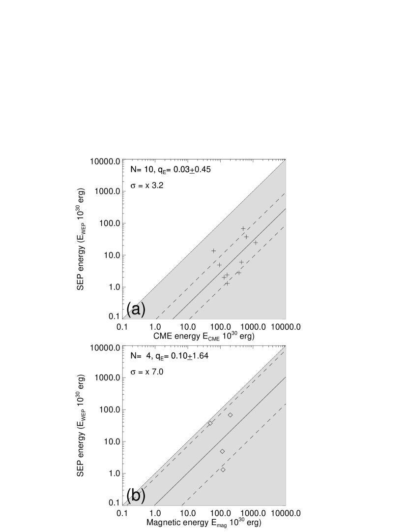
Figure 9: The ratio of SEP kinetic energies $E_{\mathrm{SEP}}$ to CME energies $E_{\mathrm{CME}}$ (a) and versus the dissipated magnetic energy $E_{\mathrm{mag}}$ in flares (b), based on the SEP data given in Table 1.

The energy range of the ten SEP events listed in Table 1 extends over $E_{\mathrm{SEP}}=(1.3-68)\times 10^{30}$ erg. If SEP events are accelerated in CME-driven shocks, they should not exceed the total CME energy. Indeed we find a ratio (Fig. 9a) of

$$E_{\mathrm{SEP}}/E_{\mathrm{CME}}=0.03\pm 0.45\ ,$$ (16)

which is comparable with the previous result of Emslie et al. (2012), i.e., $E_{\mathrm{SEP}}/E_{\mathrm{CME}}\approx 0.04$.

Comparing the SEP energy with the total dissipated magnetic energy of the flare, we have only 4 events available, which yields a large uncertainty (Fig. 9b),

$$E_{\mathrm{SEP}}/E_{\mathrm{mag}}=(0.10\pm 1.64)\ .$$ (17)

The low ratio is consistent with our notion of CME-driven acceleration leading to SEP events being a secondary energy conversion process (Fig. 1). The first step supplies the generation of a CME, while the second step drives particle acceleration in CME-driven shocks. In particular, the low ratio confirms that the magnetic free energy in the flare region is sufficient to explain the energetics of SEP particles, regardless of whether they are accelerated in the coronal flare region or in interplanetary shocks.

3 ENERGY CLOSURE

After we discussed the calculations of the various forms of energy that occur in flares and CMEs, we are now in the position to test the energy closure. We evaluate the energy closure for primary energy dissipation only (Fig. 1), by adding up the nonthermal energy in particles, $E_{\mathrm{nt}}$, the CME energy, $E_{\mathrm{CME}}$, and the direct heating energy $E_{\mathrm{dir}}$, which constitutes the right-hand part of Eq. (1), and which we denote as the sum, $E_{\mathrm{sum}}$,

$$E_{\mathrm{sum}}=(E_{\mathrm{nt}}+E_{\mathrm{dir}}+E_{\mathrm{CME}})=(E_{\mathrm{nt,e}}+E_{\mathrm{nt,i}}+E_{\mathrm{dir}}+E_{\mathrm{CME,kin}}+E_{\mathrm{CME,grav}})\ .$$ (18)

The ratio of these energy sum values $E_{\mathrm{sum}}$ and the dissipated magnetic energy $E_{\mathrm{mag}}$ is shown in Fig. 2e for all 76 events with overlapping magnetic, nonthermal, and CME data, yielding a ratio of $E_{\mathrm{sum}}/E_{\mathrm{mag}}=0.99\pm 0.19$. If we remove the outliers, as indicated by the excessive values in the tails of log-normal Gaussian distributions (Fig. 2b and 2d), we have a smaller sample with 54 events, but obtain a somewhat more accurate ratio of (Fig. 3f),

$$E_{\mathrm{sum}}/E_{\mathrm{mag}}=(0.87\pm 0.18)\ .$$ (19)

The standard deviation of the ratio is a factor of $\sigma=4.6$ (Fig. 2e), which shrinks after the elimination of outliers (Fig. 3f) to a more accurate value of $\sigma=3.2$. Thus we obtain an almost identical ratio with or without removal of outliers, but a narrower standard deviation. Our chief result is that we obtain, in the statistical average, energy closure for magnetic energy dissipation in flares by $87\%$ , with an error of $\pm 18\%$ that includes the ideal value of $100\%$ for perfect closure. This key result, demonstrated here for the first time, is visualized in form of a pie chart in Fig. 10 (right-hand side).

For comparison we show also the energy closure applied to the study of Emslie et al. (2012), as illustrated in Fig. 10 (left-hand side). That study has a smaller statistics with 37 events, which provides only 8 events with overlapping magnetic, nonthermal, and CME data, and exhibits incomplete energy closure with a value of $E_{\mathrm{sum}}/E_{\mathrm{mag}}=(0.25\pm 0.24)$ (Fig. 4f). We conclude that the overestimate of the magnetic energy $E_{\mathrm{mag}}$ and the overestimate of the low-energy cutoff $e_{c}$ in the nonthermal energy $E_{\mathrm{th}}$ are mostly responsible for the lack of energy closure in the previous study of Emslie et al. (2012).

The pie chart shown in Fig. 10 depicts that the nonthermal electron energy dissipates the largest fraction of magnetic energy, the ions dissipate the second-largest energy fraction, while the CMEs and direct heating require substantially less energy. The agreement between the energy sum and the magnetic dissipated energy varies by a standard deviation factor of $\sigma=4.6$ (Fig. 2e), which quantifies the accuracy of energy closure that we currently are able to deduce. Since the standard deviation of electron energies amounts to a factor of $\sigma=7.7$ (Fig. 2a), being the largest among all forms of energies, we suspect that the low-energy cutoff $e_{c}$ contains the largest uncertainty of all parameters measured here (although we do not know the uncertainty in the ion energy cutoff). In the largest analyzed flares, where the electron energy was found to be systematically higher than the dissipated magnetic energy (Paper III; Fig. 7 therein), our method obviously over-estimates the energy in nonthermal electrons.

Of course, there are a number of caveats, such as the lack of energy estimates for direct heating (for which no quantitative analysis method exists), or the lack of energy estimates in accelerated ions (which can only be obtained in flares with detectable gamma-ray lines and may be feasible in about 5-10 events in our data set; Albert Shih, private communication 2016).

4 DISCUSSION

Quantifying the amount of energies in the various dynamical processes that take place during a solar flare and CME allows us to to discuss which energy conversion processes are possible and which ones are ruled out, based on the available energy.

4.1 The Warm-Target Low-Energy Cutoff

We found that the nonthermal energy in electrons accelerated during a flare dissipates the largest amount of magnetic energy. This implies that the low-energy cutoff energy $e_{c}$ is the most critical parameter in the calculation of the energy budget of flares, because of the highly nonlinear dependence of the nonthermal energy on this parameter. We explicitly show this functional dependence $E_{\mathrm{nt,e}}(e_{c})$ in Fig. 11, for four different power law slopes of the hard X-ray photon spectrum ($\gamma=4-7$), corresponding to power law slopes $\delta=\gamma+1$ with a range of $\delta=5-8$ of the electron injection spectrum, according to the thick-target model (Brown 1971). From the diagram in Fig. 11 it is clear that the nonthermal energy varies by one to three orders of magnitude, depending on whether a low-energy cutoff of $e_{c}=6$ keV or $e_{c}=20$ keV is chosen. The warm-target model of Kontar et al. (2015) offers a new method to constrain this low-energy cutoff, i.e., $e_{c}=\delta k_{B}T_{e}$, but a reliable method to choose the correct temperature for the warm-target has not been established yet. This may be a difficult task, since the relevant temperature may be a mixture of cool pre-flare plasma and hot upflowing evaporating flare plasma. As a first attempt we used the DEM peak temperatures evaluated from AIA data, which yield a mean temperature of $T_{e}=8.6$ MK or $k_{B}T_{e}=0.74$ keV (Paper III). This yields then a low-energy cutoff of $e_{c}=\delta k_{B}T_{e}\approx 3.7-5.9$ keV for $\delta=5-8$. Such low values of the low-energy cutoff have dramatic consequences.

Since the warm-target offers a physical model of the low-energy cutoff, for which we infer a typical value of $e_{c}\approx 6$ keV (based on a mean temperature of $T_{e}=8.6$ MK in flaring active regions), we obtain consequently one to three orders of magnitude higher nonthermal energies in electrons, which constrains a lower limit of the energy cutoff, or an upper limit for nonthermal electron energies. Because of the highly nonlinear dependence of the nonthermal energy on the low-energy cutoff, it produces the largest uncertainty in the nonthermal energy.

The relative energy partition of nonthermal electrons is the largest difference to the study of Emslie et al. (2012), which is explained by the highly nonlinear scaling behavior of the low-energy cutoff (see Fig. 11 for estimates of the relative change in the energy partition). It dominates all other energetics, is mainly responsible for the energy closure, and together with the lower CME energies it reverses the flare-CME energy partition derived by Emslie et al. (2012), and in addition completely dominates over the thermal flare energy, in contrast to the results of Saint-Hilaire and Benz (2005) and Warmuth and Mann (2016a, b). It is clear that these new contrasting results mostly occur due to the adoption of a relatively low energy cutoff imposed by the warm-target model. For instance, the nonthermal energy for event #12 (Table 2) exceeds the dissipated magnetic energy substantially and is likely to be over-estimated due to a large error in the low-energy cutoff. Hence, the assumption of the warm-target temperature, the measurement of a representative temperature distribution in the inhomogeneous flare plasma, and its variation from flare to flare, are subject to large uncertainties, and thus add a significant caveat to our energy closure tests. In order to minimize uncertainties of the assumed warm-target temperature, we used a mean value of $T_{e}=8.6$ MK that was obtained from the emission measure weighted DEMs, averaged during the entire flare durations, and averaged from all analyzed flare events.

4.2 Sufficiency of the Thick-Target Model

In the classical (cold) thick-target bremsstrahlung model (Brown 1971), nonthermal electrons precipitate from the coronal acceleration site along the magnetic field lines towards the chromosphere, heat up the plasma in the upper chromosphere and drive upflows of heated plasma, a process that is called chromospheric evaporation. In this scenario, all nonthermal energy of the precipitating electrons is converted into the thermal energy of the evaporating plasma. Therefore, in the absence of any other heating mechanism, we expect the inequality,

$$E_{\mathrm{th}}\leq E_{\mathrm{nt}}=(E_{\mathrm{nt,e}}+E_{\mathrm{nt,i}})\ .$$ (20)

We discussed this inequality in Section 2.4 and showed that virtually all flares have a thermal energy that is substantially less than the nonthermal energy in electrons (Fig. 6), after removal of statistical outliers. This result confirms that the thick-target bremsstrahlung model is sufficient to explain the observed thermal plasma in flares.

4.3 Secondary Energy Dissipation Processes

While we discussed only the primary energy dissipation processes in Section 3, we may also consider secondary energy dissipation processes for the energy balance, which includes the generation of thermal energy, bolometric energy, and radiative energies in flares, as depicted in the diagram of Fig. 1. Ignoring the CME-related energies for the moment, most of the non-thermal energy in accelerated electrons and ions, as well as direct heating, is expected to contribute to the thermal energy $E_{th}$, based on the thick-target model and the Neupert effect, where precipitating electrons heat up the coronal warm-target regions and the upper chromosphere by the so-called chromospheric evaporation process. Interestingly, however, we measure thermal energies that amount to 12% of the non-thermal energies only (Fig. 6b). Does this imply a low efficiency of the thick-target model? There are essentially two possibilities: either the non-thermal energy in electrons is over-estimated (most likely because of the relatively low cutoff energy of 6 keV), or the thermal energy is under-estimated (mostly because we calculate the thermal energy at the flare peak time only).

On the other side, one would expect that the bolometric energy should constitute at least a major fraction of the non-thermal energy in electrons and ions, as well as the resulting thermal energy, manifested by white-light emission in deeper chromospheric layers due to locally enhanced ionization. Indeed we do find that the bolometric energy equates to the thermal energy in the statistical average ($E_{bol}/E_{th}=1.14\pm 0.05$, Fig. 8b), but there is a discrepancy that the bolometric energy does not match the non-thermal energy in electrons, estimated to be $E_{bol}/E_{nt,e}=0.07/0.51\approx 0.14$ (based on $E_{bol}/E_{mag}=0.07\pm 0.10$ and $E_{nt,e}/E_{mag}=0.51\pm 0.17$; Table 3). A good result of this estimates is that the bolometric energy approximately matches the thermal energy, consistent with other findings for very large flares, where two independent methods of determining $E_{bol}$ give a similar balance, using single events from SORCE and event ensembles from SOHO/VIRGO (Warmuth and Mann 2016a,b). We suspect that our method may over-estimate the nonthermal energy and thus yields an upper limit on the energy in non-thermal electrons, complementary to the lower limits (or under-estimates) of other earlier studies (Emslie et al. 2012).

4.4 Magnetic Reconnection Models

Our result of energy closure (Eqs. 18, 19) corroborates the conjecture that a flare with (or without) CME is of magnetic origin. Stating this result the other way round, we conclude that no other (than magnetic) energy sources are needed to produce a flare or to expel a CME. As we mentioned in Section 2.1, the dissipated magnetic energy was calculated from the twist of helical field lines in the flaring active region that is relaxed during a flare and leads to a lower (magnetic) energy state. We may ask what kind of magnetic processes are consistent with this scenario? Magnetic reconnection is most generally defined by a mutual exchange of the connectivity between oppositely polarized magnetic charges. In the case of solar flares, the magnetic charges are buried below the photospheric surface, while the coronal configuration of the magnetic field can be bipolar, tripolar, or quadrupolar. A magnetic reconnection process needs to be triggered by a magnetic instability, but evolves then from a higher to a lower energy state. This is reflected in our finding that the free energy reduces from a higher value at flare start to a lower value at flare end (Paper I). However, a puzzling observation is that often an increase of the free energy is observed immediately before flare start (Aschwanden, Xu, and Jing 2014, Paper I), which is not predicted by magnetic reconnection process. Such a feature could be produced by temporary compression or an implosion process, but is poorly understood at this point. Nevertheless, our result on the energy closure strongly confirms the role of magnetic reconnection models, and could not be explained in terms of any non-magnetic process (such as by acoustic waves or hydrodynamic turbulence).

4.5 The Acceleration Efficiency

Our result on the nonthermal energy in electrons amounting to approximately half of the dissipated magnetic energy (Eq. 5) implies a highly efficient accelerator, at least for electrons. From the statistical result of $E_{\mathrm{nt,e}}/E_{\mathrm{mag}}\approx 0.5$ (Eq. 5) obtained from our measurements we can estimate the required electron densities and magnetic fields in the acceleration region. The electron spectrum falls off steeply with energy, so that the mean kinetic energy of accelerated electrons is essentially given by the low-energy cutoff $e_{c}=(1/2)m_{e}v^{2}\approx 6$ keV $\approx 10^{-8}$ erg. Thus we obtain the total kinetic energy of all accelerated electrons by multiplying the kinetic energy of a single (nonthermal) electron with the density $n_{acc}$ of accelerated electrons and volume $V$ of the acceleration region,

$$E_{\mathrm{nt,e}}=({1\over 2}m_{e}v^{2})\ n_{acc}\ V\approx e_{c}\ n_{acc}\ V\ .$$ (21)

On the other side, the total free magnetic energy is given by the volume integral,

$$E_{\mathrm{mag}}=\left({B_{\varphi}^{2}\over 8\pi}\right)\ V\ .$$ (22)

Setting the energy ratio to the observed value, $E_{\mathrm{nt,e}}=E_{\mathrm{mag}}$ (Eq. 5) yields then for the acceleration efficiency $q_{\mathrm{acc}}$,

$$q_{\mathrm{acc}}=\left({E_{\mathrm{nt,e}}\over E_{\mathrm{mag}}}\right)=0.5\times\left({e_{c}\over 6\ {\rm keV}}\right)\left({n_{acc}\over 10^{9}\ {\rm cm}^{-3}}\right)\left({B_{\varphi}\over 22\ {\rm G}}\right)^{-2}\ .$$ (23)

Thus for a moderate potential field of $B_{p}\approx 100$ G and a twisted perpendicular component of $B_{\varphi}\approx 22$ G, which corresponds to a twist angle of $\alpha=\arctan{(B_{\varphi}/B_{p})}\approx 12^{\circ}$, we can explain electron acceleration above a low-energy cutoff of 6 keV. If we insert the measured acceleration efficiency of $q_{\mathrm{acc}}\approx 0.5$ and the associated low-energy cutoff value of $e_{c}=6$ keV, we obtain a direct relationship between the mean azimuthal magnetic field $B_{\varphi}$ and the mean electron density $n_{acc}$,

$$\left({n_{acc}\over 10^{9}\ {\rm cm}^{-3}}\right)\approx\left({B_{\varphi}\over 22\ {\rm G}}\right)^{2}\ ,$$ (24)

which provides us another testable relationship in the flaring active region. The azimuthal field component $B_{\varphi}$ can directly be measured with the vertical-current approximation nonlinear force-free field (VCA-NLFFF) code used in Paper I, while the mean electron density can be obtained from the total emission measure and flare volume as measured in Paper II. However, the spatio-temporal flare geometry has to be deconvolved into single flare loops for a proper test.

4.6 Conductive and Radiative Energy Losses

The heated solar flare plasma, which is produced by chromospheric heating from precipitating electrons and ions (and direct heating), and by subsequent chromospheric evaporation, loses its thermal energy by conductive and radiative losses in the solar corona, according to the Neupert effect. In addition, some flare plasma will be directly heated in the acceleration region (e.g., Sui and Holman 2003; Caspi and Lin 2010; Liu et al. 2013; Caspi et al. 2015), for which we can estimate a lower limit for the cases where the thermal energy excceds the nonthermal energy. Since we consider the acceleration of electrons and ions as primary energization process in our energy budget (Fig. 1), all subsequent heating and cooling processes are secondary energy conversion steps and thus are not included in the energy budget in order to avoid double-counting. These cooling processes include energy losses due to (1) thermal conduction from the corona to the chromosphere, with a energy loss rate $dE_{\mathrm{cond}}/dt\propto-T^{7/2}/L^{2}$ that tends to be most efficient for the hottest flare plasma and the shortest flare loops, and additional energy losses due to (2) radiative losses, with a radiative cooling rate of $dE_{\mathrm{rad}}/dt\propto-n_{e}^{2}T^{-3/2}$, being most efficient in the densest flare loops at lower temperatures radiating in EUV. Radiative losses in soft X-rays, calculated from the GOES fluxes, yielded a very small contribution to the total energy budget, i.e., $E_{rad}/E_{mag}=0.004\pm 0.130$ (Eq. 12, Section 2.5).

In principle the total energy losses can be computed for each flare event, but this would require to measure the time evolution of the volumetric heating rate and conductive and radiative losses with proper spatio-temporal modeling, which is not attempted in our statistical study, since radiative energy losses amount to a negligible fraction of the global flare energy budget. For more details, the reader is referred to the study of Milligan et al. (2014), where the radiated energy budget of chromospheric plasma in a major solar flare is deduced from multi-wavelength observations. We quote in Table 2 the energy values for flare #12 (2011 Feb 15, 01:46 UT; see also Fig. 3 in Paper III), along with a condensed form of Table 3 of Milligan et al. (2014), which provides the energies that are re-radiated across the visible and EUV ranges of the solar spectrum, all being in the energy range of $E_{\mathrm{rad}}\approx(10^{26}-10^{30})$ erg, and thus are fully accounted for by the dissipated magnetic energies derived here.

Although one would expect in the thick-target model that the total radiative energy loss cannot exceed the thermal energy, there is the possibility that continuous energy input (by nonthermal particles and direct heating) into the flare plasma after the flare peak can boost the radiative energy above the thermal energy, especially in large events. Both Emslie et al. (2012) and Warmuth and Mann (2016a,b) found that the radiated energy of the hot plasma can be slightly higher than the maximum thermal energy, while Warmuth and Mann (2016a,b) deduced conductive losses that were significantly larger than the peak thermal energies. If this is the case, radiative losses could possibly add a non-negligible fraction to the global energy budget.

5 CONCLUSIONS

This study is the first attempt to investigate energy closure in solar flare and CME events. All the arguments made here are based on the various forms of energies as measured in a series of recent studies, which include the magnetic energy (Paper I), the thermal energy (Paper II), the nonthermal energy (Paper III), and CME energies (Paper IV). We arrive at the following conclusions:

1. Energy Closure: From the temporal causality that is inherent in the most commonly used physical models of flare and CME processes we distinguish between primary and secondary energy dissipation processes, but test mainly the energy closure of the primary step, which includes the dissipation of free magnetic energy $E_{\mathrm{mag}}$ to support acceleration of particles (electrons and ions) with a total nonthermal energy $E_{\mathrm{nt}}=E_{\mathrm{nt,e}}+E_{\mathrm{nt,p}}$, direct heating of flare plasma $E_{\mathrm{dir}}$, and the simultaneous launch of a CME with a kinetic and gravitational potential energy $E_{\mathrm{CME}}=E_{\mathrm{CME,kin}}+E_{\mathrm{CME,grav}}$. Thus, the expected energy closure in the primary flare dissipation process is the equivalence between the dissipated magnetic energy $E_{\mathrm{mag}}$ and the sum of the first-step energy dissipation processes, $E_{\mathrm{sum}}=E_{\mathrm{nt}}+E_{\mathrm{dir}}+E_{\mathrm{CME}}$. Our chief result is the finding of equivalence in the statistical mean, within the statistical uncertainties, namely $E_{\mathrm{sum}}/E_{\mathrm{mag}}=0.87\pm 0.18$, with a standard deviation factor of $\sigma=3.2$ for individual flare/CME events. If we restrict the statistics to a subset of 76 events by eliminating outliers, we find an energy closure of $E_{\mathrm{sum}}/E_{\mathrm{mag}}=0.99\pm 0.19$ (Fig. 2e).

2. Energy Partition in the primary flare energy budget: Comparing the mean ratios of the various primary energy dissipation processes with the dissipated magnetic energy (100%), we find in the statistical average, that 51% of the magnetic energy goes into nonthermal electrons, 17% into nonthermal ions, 7% into the launch of a CME, 7% into direct heating of flare plasma, and 18% is the residual that may include alternative energy dissipation processes or statistical errors. Since the analyzed data set is a complete sample of all flares with GOES class $\geq M1$, it is dominated by mid-size ($\;\buildrel>\over{\scriptstyle\sim}\;$ M1.0) flares.

3. The thermal/nonthermal energy ratio: We find a relatively low ratio of thermal to nonthermal energies, i.e., $E_{\mathrm{th}}/E_{\mathrm{nt,e}}=0.12\pm 0.11$. This result is consistent with the thick-target bremsstrahlung model (Brown 1971) in the sense that the precipitating nonthermal electrons contain sufficient energy to heat up the upper chromosphere and to drive chromospheric evaporation to produce the observed thermal energy in SXR and EUV. On the other side, for an ideal thick-target model we would expect near-equivalence of thermal and nonthermal energies. We suspect that this low energy conversion efficiency is caused by combination of over-estimated nonthermal energies in electrons, and under-estimated thermal energies due to neglecting multiple (secondary) heating episodes and simultaneous conductive and radiative losses.

4. The bolometric/thermal energy ratio: White-light emission appears in all large flares and is highly correlated with the SXR flux. We find an energy ratio of $E_{\mathrm{bol}}/E_{\mathrm{th}}=1.14\pm 0.05$ between the bolometric energy and the thermal energy, using the scaling law of Kretzschmar (2011) between the bolometric luminosity and the GOES SXR flux. The flare-associated SXR flux is believed to be produced mostly by precipitating particle beams (due to the generation of hot plasma by chromospheric evaporation), which may cause enhanced ionization and excitation of white-light flare emission as well.

5. The SEP/CME energy ratio: Based on the SEP analysis of a small subset of 8 events we find a (logarithmic mean) ratio of $E_{\mathrm{SEP}}/E_{\mathrm{CME}}=0.03\pm 0.45$ between the energy in SEPs and CMEs. This result corroborates the conjecture that SEP particles are primarily accelerated by CME-driven shocks, with an acceleration efficiency in the order of a few percents. Of course, this does not eliminate a possible acceleration of SEPs at the coronal flare site.

6. The warm-target concept provides a physical model for estimating a lower limit of the low-energy cutoff $e_{c}$, or an upper limit on the nonthermal energies, which scales with the temperature $T_{e}$ of the warm-target plasma and the power law slope $\delta$ of the nonthermal spectrum. Using the DEM peak temperature of a large sample of M- and X-class flares yields a mean temperature of $T_{e}=8.6$ MK and a low-energy cutoff value of $e_{c}\approx 6$ keV, which is substantially below earlier estimations of $e_{c}\approx 20$ keV and produces about one to three orders of magnitude higher nonthermal energies. Because of the highly nonlinear dependence of the nonthermal energy on the low-energy cutoff, it produces the largest uncertainty in the nonthermal energy and in the energy closure relationship.

Energy closure constitutes a rigorous quantitative test whether our physical models of dynamic phenomena are complete and accurate, or whether we miss important first-order effects. In our study on solar flares and CMEs we fortunately find energy closure for (nonpotential) magnetic energies that supply the creation of a flare and the launch of a CME, which is a strong endorsement for magnetic reconnection models. From the inequality relationships of secondary energy dissipation processes we also find strong support for the thick-target model, the warm-target model, flare-associated chromospheric white-light emission, and CME-driven shocks, but we encountered large uncertainties up to an order of magnitude in some of the calculated energies, in particular for the nonthermal energy that depends in a highly nonlinear manner on the low-energy cutoff. In addition, there are number of flare aspects that we do not understand at this time, for instance: (1) The direct heating in flares that accompanies particle acceleration; (2) The physics of various particle transport and acceleration processes; and (3) The thermal evolution and shock-driven acceleration in CMEs. Future modeling, using the powerful tool of energy closure criteria applied here, may further help to discriminate various physical flare and CME models.

Table 1: SEP kinetic energies for selected 3-spacecraft events from 2011-2013. The higher value of the two lower limits of CME/LASCO (column 6) and CME/AIA energies (column 7) is used in the SEP/CME ratio (column 8).

#	Flare	GOES	Heliographic	SEP kinetic	CME/LASCO	CME/AIA	SEP/CME
	Date	class	position	energy	energy	energy	energy ratio
				$(10^{30}$ erg)	$(10^{30}$ erg)	$(10^{30}$ erg)
12	2011-Feb-15	X2.2	S21W12	1.3	$>$1.6	161.0	0.008
58	2011-Aug-04	M9.3	N18W36	4.9	45.0	$>$15.0	0.110
74	2011-Sep-22	X1.4	N08E89	2.8	265.0	$>$14.0	0.011
102	2011-Oct-22	M1.3	N27W87	13.6	22.0	$>$17.0	0.620
131	2012-Jan-23	M8.7	N33W21	37.3	413.0	$>$19.0	0.090
132	2012-Jan-27	X1.7	N33W85	24.5	819.0	$>$41.0	0.030
148	2012-Mar-07	X1.3	N18E29	67.6	362.0	$>$12.0	0.190
169	2012-May-17	M5.1	N07W88	6.0	251.0	$>$14.0	0.024
284	2013-May-13	X1.7	N11W89	2.0	61.0	$>$11.0	0.033
296	2013-Jun-21	M2.9	S14E73	2.4	100.0	$>$12.0	0.024
	Logarithmic	mean					0.03$\div$3.2

Table 2: Wavelength ranges and energies of the 2011 Feb 15, 01:46 UT, GOES X2.2 flare, as derived for magnetic energies (see Table 3 in Paper I), the thermal energy (see Table 2 in Paper II), the nonthermal energy (see Table 1 in Paper III), the CME energies (see Table 3 in Paper IV), and radiative energies determined by Milligan et al. (2014).

	Wavelength range	Energy
	(Å)	(erg)
Magnetic potential energy	6173, 94-305	$(1065\pm 14)\times 10^{30}$
Magnetic free energy	6173, 94-305	$(52\pm 20)\times 10^{30}$
Magnetic dissipated energy	6173, 94-305	$(120\pm 10)\times 10^{30}$
Thermal energy	94-305	$82\times 10^{30}$
Nonthermal energy	0.25-2.1	$1100\times 10^{30}$
CME kinetic energy	94-305	$124\times 10^{30}$
CME gravitational energy	94-305	$40\times 10^{30}$
Ly $\alpha$ line	1170-1270	$(1.2\pm 0.3)\times 10^{30}$
He II line	302.9-304.9	$(3.4\pm 0.1)\times 10^{29}$
UV continuum	1600-1740	$2.6\times 10^{29}$
C IV line + UV continuum	1464-1609	$1.7\times 10^{29}$
Lyman continuum	504-912	$(1.8\pm 1.0)\times 10^{29}$
Ca II H line	3967-3970	$5.5\times 10^{28}$
He I continuum	370-504	$(3.0\pm 0.6)\times 10^{28}$
He II continuum	200-228	$1.6\times 10^{28}$
Green continuum	5548-5552	$1.5\times 10^{26}$
Red continuum	6682-6686	$1.4\times 10^{26}$
Blue continuum	4502-4506	$1.2\times 10^{26}$

Table 3: Summary table of statistical energy ratios in flares. The sum of primary energies includes nonthermal electrons, ions, direct heating, and CME (kinetic and potential) energies.

Energy type	Number of	Fraction of	Number of	Fraction of
type	flares	magnetic energy	flares	thermal energy
Free magnetic energy	172	$E_{\mathrm{mag}}/E_{\mathrm{mag}}=1.00\pm 0.00$
Nonthermal electrons	55	$E_{\mathrm{nt,e}}/E_{\mathrm{mag}}=0.51\pm 0.17$
Nonthermal ions	55	$E_{\mathrm{nt,i}}/E_{\mathrm{mag}}=0.17\pm 0.17$
CME energy	157	$E_{\mathrm{CME}}/E_{\mathrm{mag}}=0.07\pm 0.14$
SEP energy	4	$E_{\mathrm{SEP}}/E_{\mathrm{mag}}=0.10\pm 1.64$
Direct heating	106	$E_{\mathrm{dir}}/E_{\mathrm{mag}}=0.07\pm 0.17$
Thermal energy	170	$E_{\mathrm{th}}/E_{\mathrm{mag}}=0.08\pm 0.13$	391	$E_{\mathrm{th}}/E_{\mathrm{th}}=1.00\pm 0.00$
Radiated energy in SXR	171	$E_{\mathrm{rad}}/E_{\mathrm{mag}}=0.004\pm 0.130$	389	$E_{\mathrm{rad}}/E_{\mathrm{th}}=0.07\pm 0.06$
Bolometric energy	172	$E_{\mathrm{bol}}/E_{\mathrm{mag}}=0.07\pm 0.10$	391	$E_{\mathrm{bol}}/E_{\mathrm{th}}=1.14\pm 0.05$
Sum of primary energies	52	$E_{\mathrm{sum}}/E_{\mathrm{mag}}=0.87\pm 0.18$

Figure 10: Pie chart of energy closure, obtained from previous work of Emslie et al. (2012) (left panel), and from this study (right panel).

Figure 11: The dependence of the nonthermal energy in electrons $E_{\mathrm{nt,e}}$ on the low-energy cutoff $e_{c}$, calculated for four different power law slopes $(\gamma=4-7)$ of the hard X-ray photon spectrum. Two typical low-energy cutoffs are marked: 6 keV assumed for the warm-target model, and 20 keV as typical value of the cross-over energy (Paper III).

References

- (1)
- (2)
- (3) Andrews, M.D. 2003, Solar Phys. 218, 261.
- (4) Antonucci, E. and Dennis, B.R. 1983, Solar Phys. 86, 67.
- (5) Aschwanden, M.J. 2002, Space Science Rev., 101, 1.
- (6) Aschwanden, M.J., Nitta,N.V., Wuelser,J.-P., Lemen,J.R., Sandman,A., Vourlidas,A., and Colaninno,R.C. 2009, ApJ 706, 376.
- (7) Aschwanden, M.J. 2013, Solar Phys. 287, 369.
- (8) Aschwanden, M.J., Boerner, P., Schrijver, C.J., and Malanushenko, A. 2013, Solar Phys. 283, 5.
- (9) Aschwanden, M.J., Xu, Y., and Jing, J. 2014, ApJ 797, 50, [Paper I].
- (10) Aschwanden, M.J., Boerner, P., Ryan, D., Caspi, A., McTiernan, J.M., and Warren, H.P. 2015a, ApJ 802, 53, [Paper II].
- (11) Aschwanden, M.J., Boerner, P., Caspi, A., McTiernan, J.M., Ryan, D., and Warren, H.P. 2015b, Solar Phys. 290, 2733.
- (12) Aschwanden, M.J., Holman, G., O’Flannagain, A., Caspi, A., McTiernan, J.M., and Kontar, E.P. 2016, (in press), [Paper III].
- (13) Aschwanden, M.J. 2016a, ApJ 831, 105, [Paper IV].
- (14) Aschwanden, M.J. 2016b, ApJSS 224, 25.
- (15) Atkinson, G. 1978, JGR 83, 1089.
- (16) Battaglia, M., Kontar, E.P., Hannah, I.G. 2011, A&A 526, A3.
- (17) Battaglia, M. and Kontar,E.P. 2011, ApJ 735, 42.
- (18) Benz, A.O. 2008, Living Rev. Solar Phys. 5, 1.
- (19) Boerner, P.F., Testa, P., Warren, H., Weber, M.A., and Schrijver, C.J. 2014, Solar Phys. 289, 2377.
- (20) Brown, J.C. 1971, Solar Phys. 18, 489.
- (21) Cargill, P.J., Mariska, J.T., and Antiochos, S.K. 1995, ApJ 439, 1034.
- (22) Caspi, A. 2010, PhD Thesis, University of Berkeley.
- (23) Caspi, A., and Lin, R.P. 2010, ApJ 725, L161.
- (24) Caspi, A., McTiernan, J.M., and Warren, H.P. 2014, ApJ 788, L31.
- (25) Caspi, A., Shih, A.Y., McTiernan, J.M., and Krucker, S. 2015, ApJ 811, L1.
- (26) Chollet, E.E., Giacalone, J., and Mewaldt, R.A. 2010, JGR 115, 6101.
- (27) Cox, D.P. and Tucker, W.H. 1969, ApJ 157, 1157.
- (28) Del Zanna, G., Dere, K.P., Young, P.R., Landi, E., and Mason, H.E. 2015, A&A 582, A56.
- (29) Dere, K.P., Landi, E., Mason, H.E., Monsignori Fossi, B.C. and Young, P.R. 1997, A&A 125, 149.
- (30) Ding, M.D., Liu, Y., Yeh, C.-T., and Li, J.P. 2003, A&A 403, 1151.
- (31) Emslie, A.G., Dennis, B.R., Shih, A.Y., Chamberlin, P.C., Mewaldt, R.A., Moore, C.S., Share, G.H., Vourlidas, A., and Welsch, B.T. 2012, ApJ 759, 71.
- (32) Feldman, U. Mandelbaum, P., Seely, J.F., Doschek, G.A., and Gursky, H. 1992, ApJSS 81, 387.
- (33) Holman, G.D., Aschwanden, M.J., Aurass, H., Battaglia, M., Grigis, P.C., Kontar, E.P., Liu, W., Saint-Hilaire, P., and Zharkova,V.V. 2011, SSRv 159, 107.
- (34) Hudson, H. 1972, Solar Phys. 24, 414.
- (35) Hudson, H. and Ryan, J. 1995, Ann.Rev.Astron.Astrophys. 33, 239.
- (36) Kontar, E.P., Jeffrey, N.L.S., Emslie, A.G., and Bian ,N.H. 2015, ApJ 809, 35.
- (37) Kretzschmar, M., Dudok de Wit, T., Schmutz, W., Mekaoui, S., Hochedez, J.-F., and Dewitte, S. 2010, Nature Physics, 6, 690.
- (38) Kretzschmar, M. 2011, A&A 530, A84.
- (39) Lario, D., Kallenrode, M.-B., et al. 2006, ApJ 653, 1531.
- (40) Lario, D., Aran, A., Gomez-Herrero, R., Dresing, N., Ho., G.C., Decker, R.B., and Roelof, E.C. 2013, ApJ 767, 41.
- (41) Lin, R.P. 2007, Space Science Rev. 124, 233.
- (42) Liu, W., Chen, Q., and Petrosian, V. 2013, ApJ 767, 168.
- (43) Mason, G.M., Mazur, J.E., Dwyer, J.R., Jokipii, J.R., Gold, R.E., and Krimigis, S.M., 2004, ApJ 606, 555.
- (44) Mazzotta, P., Mazzitelli, G., Colafrancesco, S., and Vittorio, N. 1998, A&AS 133, 403.
- (45) Mason,J.P., Woods, T.N., Caspi, A., Thompson, B.J., and Hock, R.A. 2014, ApJ 789, 61.
- (46) Mason,J.P., Woods, T.N., Webb, D.F., Thompson, B.J., Colaninno, R.C. and Vourlidas, A. 2016, ApJ 830, 20.
- (47) Mewaldt, R.A., Chollet, E., Cohen, C., Looper, M., Glenn, M., Vourlidas, A., Giacalone, J., et al. 2008a, 37th COSPAR Scientific Assembly, Paper D23-0018-08.
- (48) Mewaldt, R.A., Cohen, C.M., Labrador, A.W., Leske, R.A., Stone, E.C., von Rosenvinge, T.T., and Wiedenbeck, M.E. 2004, 35th COSPAR Scientific Assembly, p.2389.
- (49) Mewaldt, R.S., Cohen, C.M.S., Giacalone, J., Mason, G.M., Chollet, E.E., Desai, M.I., Haggerty, D.K., Looper, M.D., Selesnick, R.S., and Vourlidas, A. (2008b), Conference, (eds. G. Li et al.), AIP Conf. Proc. #1039, AIP, p.111.
- (50) Miller, J.A., Cargill, P.J., Emslie, A.G., Holman, G.D., Dennis, B.R., LaRosa, T.N., Winglee, R.M., Benka, S.G., and Tsuneta,S. 1997, JGR 102/A7, 14631.
- (51) Milligan, R.O., Kerr, G.S., Dennis, B.R., Hudson, H.S., Fletcher, L., Allred, J.C., Chamberlin, P., Ireland, J., Mathioudakis, M., and Keenan, F.P. 2014, ApJ 793, 70.
- (52) Najita, K. and Orrall, F.Q. 1970, Solar Phys. 15, 176.
- (53) Racusin, J.L., Liang, E.W., Burrows, D.N., Falcone, A., Sakamoto, T., Zhang, B.B., Zhang, B., and Evans, P. 2009, ApJ 698, 43.
- (54) Reames, D.V. 2013, Space Science Rev. 175, 53.
- (55) Richardson, I.G., von Rosenvinge, T.T., Cane, H.V., et al. 2014, Solar Phys. 289, 3059.
- (56) Ryan, D.F., Milligan, R.O., Gallagher, P.T., Dennis, B.R., Tolbert, A.K., Schwartz, R.A., and Young, C.A. 2012, ApJSS 202, 11.
- (57) Ryan, D.F., O’Flannagain, A.M., Aschwanden, M.J., and Gallagher,P.T. 2014, Solar Phys. 289, 2547.
- (58) Saint-Hilaire, P. and Benz, A.O. 2005, A&A 435, 743.
- (59) Schrijver, C.J, DeRosa, M.L., Metcalf, T., Barnes, G., Lites, B., Tarbell, T., McTiernan, J., Valori, G. et al. 2008, ApJ 675, 1637.
- (60) Shih, A.Y., Lin, R.P., and Mith, D.M. 2009, ApJ 698, L152.
- (61) Shih, A.Y.-M. 2009, PhD thesis, Univ. California.
- (62) Sui, L. and Holman, G.D. 2003, ApJ 596, L251.
- (63) Thomas, R.J., Crannell, C.J., and Starr, R. 1985, Solar Phys. 95, 323.
- (64) Török, T. and Kliem, B. 2005, ApJ 630, L97.
- (65) Warmuth A. and Mann G. 2016a, A&A 588, A115.
- (66) Warmuth A. and Mann G. 2016b, A&A 588, A116.
- (67) White, S.D.M., Navarro, J.F., Evrard, A.E., and Frenk, C.S. 1993, Nature Vol. 366, Issue 6454, pp.429.
- (68) White, S.M., Thomas, R.J., and Schwartz, R.A. 2005, Solar Phys. 227, 231.
- (69) Woods, T.N., Eparvier, F.G., Fontenla, J., Harder, J., Kopp, G., et al. 2004, GRL 31, L10802.
- (70) Woods, T.N., Kopp, G., and Chamberlin, P.C. 2006, JGR (Space Physics), 111, 10.
- (71) Xu, Y., Jing, J., Wang, S., and Wang, H. 2014, ApJ 787, 7.
- (72) Zilitinkevich,S.S., Elperin, T., Kleeorin, N., and Rogachevskii, I. 2007, Boundary-Layer Meteorology 125/2, 167.