Eigenmodes of 3-D magnetic arcades in the Sun’s corona
Abstract
We develop a model of coronal-loop oscillations that treats the observed bright loops as an integral part of a larger 3-D magnetic structure comprised of the entire magnetic arcade. We demonstrate that magnetic arcades within the solar corona can trap MHD fast waves in a 3-D waveguide. This is accomplished through the construction of a cylindrically symmetric model of a magnetic arcade with a potential magnetic field. For a magnetically dominated plasma, we derive a governing equation for MHD fast waves and from this equation we show that the magnetic arcade forms a 3-D waveguide if the Alfvén speed increases monotonically beyond a fiducial radius. Both magnetic pressure and tension act as restoring forces, instead of just tension as is generally assumed in 1-D models. Since magnetic pressure plays an important role, the eigenmodes involve propagation both parallel and transverse to the magnetic field. Using an analytic solution, we derive the specific eigenfrequencies and eigenfunctions for an arcade possessing a discontinuous density profile. The discontinuity separates a diffuse cylindrical cavity and an overlying shell of denser plasma that corresponds to the bright loops. We emphasize that all of the eigenfunctions have a discontinuous axial velocity at the density interface; hence, the interface can give rise to the Kelvin-Helmholtz instability. Further, we find that all modes have elliptical polarization with the degree of polarization changing with height. However, depending on the line of sight, only one polarization may be clearly visible.
1 Introduction
The loops of bright plasma revealed in EUV images of the solar corona often sway back and forth in response to nearby solar flares (e.g., Aschwanden et al. 1999; Nakariakov et al. 1999). A flurry of observational and theoretical efforts has been devoted to the explanation and exploitation of these oscillations (see the review by Andries et al., 2009). In particular, the detection of multiple, co-existing frequencies (Verwichte et al., 2004; Van Doorsselaere et al., 2007; De Moortel & Brady, 2007) has encouraged the hope that seismic methods might be developed to measure loop properties, as first suggested by Roberts et al. (1984). However, before seismic techniques can be fruitfully applied, we must have a firm grasp on the nature of the wave cavity in which the waves reside. A commonly accepted viewpoint is that each visible loop is a separate wave cavity for MHD kink waves. The waves are presumed to have a group velocity that is parallel to the axis of the magnetic field and each loop oscillates as a coherent, independent entity. Thus, the problem can be reduced to a 1-D wave problem with boundary conditions at the two foot points of the loop in the photosphere.
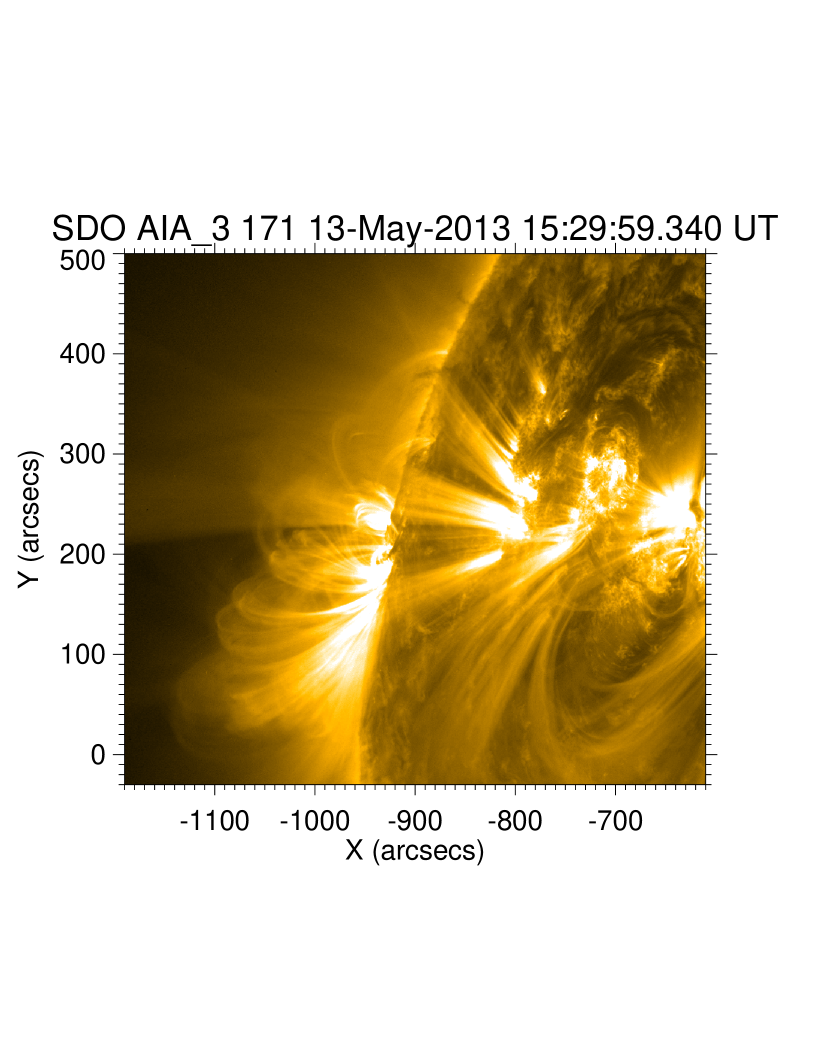
There are several lines of evidence that suggest that the entire 3-D magnetic arcade in which the bright loops reside participates in the oscillation. Thus, the true wave cavity is much larger than the individual loop and probably multi-dimensional. One of these lines of evidence comes from viewing an arcade on the limb where the loops have higher visibility (see Figure 1). With high cadence data from TRACE and AIA, it is clear that multiple loops within a single magnetic arcade often oscillate in concert (Verwichte et al., 2009; Jain et al., 2015). Further, one sees oscillations traveling down the axis of the arcade, crossing from one loop top to another, almost perpendicular to the field lines. To see for yourself, we suggest that the reader should examine the ancillary file, which consists of an animation of AIA images that shows the response of a magnetic arcade to a flare. The first frame of this animation appears is shown separately as Figure 1.
A second line of evidence comes from the power spectrum of the oscillations. Jain et al. (2015) observed a pair of loops embedded within a common arcade. From the time series of loop positions, they found that the spectral power was sharply peaked around the oscillation frequency, but with a noticeable enhancement of the high-frequency wing of the peak compared to the low-frequency wing. Any scattering process usually results in symmetric broadening of the power peak. Therefore, Jain et al. (2015) suggest that the asymmetry in the power spectrum is evidence for the existence of a 2D or 3D waveguide with a continuum of eigenmodes propagating transverse to the field as well as parallel. Each of the modes with transverse propagation has a higher frequency than the mode with purely parallel propagation. Hence the integral over all possible transverse wavenumbers results in preferential enhancement of the high-frequency wing of the spectral peak. Such asymmetry was previously predicted in a theoretical model by Hindman & Jain (2014) who explored the propagation of fast MHD waves within a 2-D waveguide.
Our goal here is to perform the initial theoretical analysis demonstrating that magnetic arcades form 3-D waveguides and to elucidate the basic properties of the resulting 3-D wave modes. In section 2, we present a simple model that treats a magnetic arcade as a cylindrically symmetric, potential magnetic field. In section 3, we develop general governing equations for fast MHD waves within the prescribed magnetic field. In Section 4, we present and discuss an analytic solution for the eigenmodes for special profiles of the mass density and Alfvén speed. Finally, in section 5, we discuss the observational implications of our work.
2 Model of a coronal arcade as a magnetized cylinder
A coronal loop is believed to be bright because preferential heating on a thin bundle of field lines causes hot, dense plasma to fill that bundle. Therefore, an arcade of bright loops is probably a magnetic structure where a density inversion has occurred. A dim cavity of diffuse magnetized plasma underlies a thin region of dense overlying fluid which radiates profusely, creating the visible loops. Thus, when modeling a coronal loop, one should attempt to construct a model that possesses a density enhancement suspended within the corona.
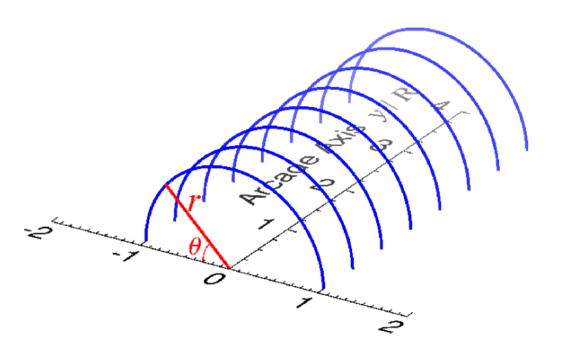
We choose to keep the magnetic field itself relatively simple and consider a 3-D model which assumes that the magnetic field lines form a set of semi-circular arches. The magnetic structure possesses cylindrical geometry with the axis of the cylinder pointing horizontally and embedded in the photospheric plane. The half of the cylinder lying above the photosphere corresponds to the arcade, with the field lines being circles centered on the axis. We define a cylindrical coordinate system (, , ) whose axis is co-aligned with the axis of the arcade. The axial coordinate is , the distance from the axis is , and the angle between the position vector and the photospheric plane is . The range of azimuths lies above the photosphere.
The magnetic field is purely toroidal and force free. The only field that meets these two conditions is the potential field generated by a line current of strength located on the axis,
| (2.1) |
The field strength is a decreasing function of radius that only depends on radius. Figure 2 illustrates the magnetic geometry.
3 Governing Wave Equations
If we assume that the plasma is magnetically dominated, so that we can safely ignore gas pressure and buoyancy forces, the wave motions become purely transverse because the Lorentz force itself is transverse. Therefore, the azimuthal component, , of the fluid’s velocity vector will be identically zero, and only the radial and axial components are nonzero, . For such transverse motions, the induction equation dictates that the fluctuating magnetic field is as follows:
| (3.2) | |||||
| (3.3) |
The variable is proportional to the temporal derivative of the magnetic-pressure fluctuation, ,
| (3.4) |
For the magnetically dominated plasma discussed previously, the MHD momentum equation takes on a relatively simple form,
| (3.5) |
where is the Alfvén speed and is the component of the gradient operator that is transverse to the magnetic field,
| (3.6) |
In equation (3.5) the term involving represents the effects of magnetic pressure forces and the two terms in parentheses comprise the magnetic tension.
In order to ensure that equation (3.5) is tractable and has separable solutions, we assume that the Alfvén speed is a function of radius alone, . Since the magnetic-field strength is also a function of only radius, , the mass density must also vary only with radius, . This density variation is consistent with hydrostatic balance along field lines as long as the corona is exceedingly hot such that the density scale height due to gravitation is much larger than the height of the loops in the arcade.
For an atmosphere possessing the cylindrical symmetry discussed above, the eigensolutions to equation (3.5) have a separable form,
| (3.7) |
In this expression, is the temporal frequency, is the axial wavenumber, and is the azimuthal order. We have selected this solution in order to satisfy a line-tying boundary condition (i.e., stationary field lines) at the photosphere ( and ). Further, we have also assumed that the arcade is sufficiently long in the axial -direction that we can ignore edge effects and presume invariance in the coordinate. Hence, the eigenfunctions are propagating waves in the -direction. We recognize that this assumption is problematic for many arcades, but we adopt it despite these reservations for reasons of tractability and simplicity of argument.
Given solutions with the separable form posited by equation (3.7), the two components of equation (3.5) become a set of coupled ODEs,
| (3.8) | |||||
| (3.9) | |||||
| (3.10) |
These equations can be combined into a single ODE for the variable ,
| (3.11) |
where is a scale length
| (3.12) |
Depending on the profile of the Alfvén speed as a function of radius, , equation (3.11) may possess turning points and critical points. If turning points exist, there is a possibility that the arcade forms a waveguide. For example, there might be two turning radii between which the waves are trapped. In such a circumstance, each eigenmode would be a standing wave in radius and azimuth , while being a propagating wave in the axial coordinate . The nature of this type of waveguide will be discussed more fully when we consider specific Alfvén speed profiles in section §4.2.
Potential critical points correspond to cylindrical sheets where the Alfvén resonance condition is satisfied,
| (3.13) |
Since the scale length is divergent at these resonances, the coefficient of the first-order derivative term in equation (3.11) becomes singular at these critical radii. Critical layers of this sort often act as internal reflecting or scattering interfaces. However, since our subsequent arcade models will be intentionally constructed such that no critical radii exist, we defer further exploration of their behavior.
4 Analytic Solution
In order to provide a specific example of the waveguides that can form within these magnetic arcades, we present an analytic solution to equation (3.11). First, we note that if the waves are to be trapped in the radial direction, the Alfvén speed must increase monotonically beyond a fiducial radius. This is necessary so that refraction occurs and turns outward propagating waves back toward the interior. This places a restriction on the density profile of any model atmosphere that one proposes. Since, the magnetic-field strength decreases as , in order for the Alfvén speed to increase with radius, the density must decrease with radius faster than .
The analytic solution that we present here is predicated on the removal of all critical radii and is accomplished by specifying a particular profile for the Alfvén speed. Consider an Alfvén speed profile that increases linearly with cylindrical radius (thus satisfying the condition required for a refractive turning point). For such a profile, the Alfvén resonances disappear, the density decreases with radius as , and the scale length disappears from equation (3.11),
| (4.14) | |||||
| (4.15) | |||||
| (4.16) |
In these expressions, and are constant reference values that provide the constant of proportionality such that at radius . Since the reciprocal of vanishes, the ODE describing the radial behavior of the eigenfunctions can be recognized as a modified Bessel function equation,
| (4.17) |
where the order is potentially imaginary for sufficiently high frequency ,
| (4.18) |
The two linearly independent solutions for are just the modified Bessel functions and . The velocity components can be derived from the dimensionless pressure fluctuation, , by using equations (3.8) and (3.9),
| (4.19) | |||||
| (4.20) |
4.1 Nature of the Solutions
The order of the modified Bessel functions can be either purely real or purely imaginary and there is a transition frequency that marks the change between real and imaginary values. For low frequencies, , the order is purely real, while for high frequencies, , the order is purely imaginary. For real orders, the modified Bessel function is the solution that remains finite as , whereas the modified Bessel function diverges. At the origin, the Bessel function remains finite and the Bessel function diverges. However, for imaginary order, the Bessel function is a real function, it vanishes at infinity, and is finite but recessive at the origin. The recessive behavior (i.e., oscillatory with an infinite number of zeros on the approach to the origin) arises because the wave speed vanishes at the accumulation point. The Bessel function is a complex function when the order is imaginary and is rather badly behaved. If needed, an additional real solution can be constructed by taking a specific linear combination of modified Bessel functions. This new real function is known as the modified Bessel function (Dunster, 1990),
| (4.21) |
For imaginary order , the Bessel function has the properties that it is divergent at infinity but remains finite at the origin; although like the Bessel function, it is recessive with an infinite number of zeros piling up at the origin. We note that neither of these solutions is particularly realistic because of the recessive behavior at the origin. However, if we had permitted the Alfvén speed to remain nonzero at the origin, these difficulties would have been automatically avoided. In section §4.2, we solve this problem in another manner by constructing piece-wise continuous models of the atmosphere such that the waves are excluded from the origin by enforcing their evanescence in the inner shell.
The behavior of these solutions can be predicted and more fully understood by deriving a local radial wavenumber for equation (4.17). We do this by performing a change of variable, , such that the transformed equation becomes a Helmholtz equation lacking a first derivative term,
| (4.22) |
The local radial wavenumber can be read-off from this equation and, if expressed in terms of frequency instead of , we find
| (4.23) | |||||
| (4.24) |
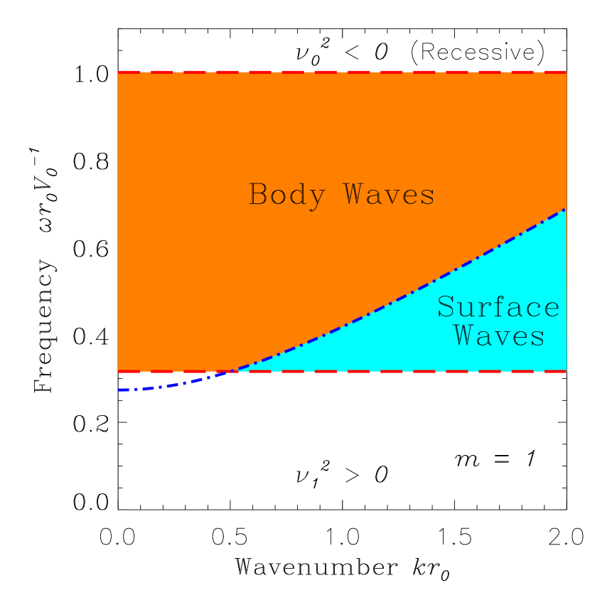
This local dispersion relation has been written in terms of a spatially constant (-dependent) cut-off frequency, . High frequency waves, , propagate, while low frequency waves, , are evanescent. Figure 3 provides a propagation diagram that illustrates those combinations of frequency and axial wavenumber that correspond to propagating waves and those associated with evanescent waves.
From the local wavenumber we can immediately deduce that there can only be one turning point and it is located at
| (4.25) |
Thus, we only have oscillatory solutions if (or equivalently ). The extent of the waveguide, or the regime of propagation, will span the range , because there is only one turning point. We can further deduce that the solutions will be recessive at the origin by noting that the local radial wavenumber is divergent as (i.e., the local wavelength vanishes at the origin).
4.2 A Waveguide Comprised of Two Shells
Since our goal here is to examine loop models that consist of a density enhancement suspended above a diffuse cavity, we choose to construct a piece-wise continuous model that is comprised of two cylindrical shells joined at . Each shell possesses the Alfvén speed profile that permits the analytic solution, but there is a pycnocline at the cylindrical interface between the two shells. This interface is currentless such that the magnetic field is continuous and unmodified from equation (2.1). However, the Alfvén speed and mass density are discontinuous at the interface and given by
| (4.28) | |||||
| (4.31) |
where is the reference speed in the inner region () and is the reference speed in the outer region ().
Since the Alfvén speed drops as increases across the interface (i.e., ), the cut-off frequency, , is larger in the inner shell than it is in the outer shell—see equation (4.24). This has the salutary property that there exists a band of frequencies for which the solutions are evanescent in the inner shell and potentially propagating in regions of the outer shell. Thus, we have the possibility of trapped waves that lack recessive behavior at the origin. Since the cut-off frequencies differ in the two regions, the order of the Bessel functions in the inner region, , and in the outer region, , also differ, .
A transcendental dispersion relation can be derived for this model by requiring the continuity of both the magnetic pressure and the radial velocity across the interface at . However, we must first choose the proper solutions within the two regions such that boundary conditions at and are satisfied. In order to avoid divergent or recessive solutions at the origin, the solution within the inner region must correspond to an modified Bessel function and the order in that region must be purely real (i.e., ). This places an upper bound on the mode frequencies,
| (4.32) |
Similarly, a boundary condition of finiteness as selects the proper solution in the outer region. The only solution that remains finite in this limit is the modified Bessel function and it does so for either real or imaginary order .
Given that the solution must be an function for and a function for , the continuity of magnetic pressure and radial velocity mandate the following dispersion relation,
| (4.33) |
and eigenfunction
| (4.34) |
where the primes indicate differentiation with respect to the argument of the Bessel function and is a normalization constant.
If one assumes a priori that one can quickly demonstrate that the left-hand side of equation (4.33) is negative and the right-hand side is positive. Hence, a contradiction occurs and only solutions with are allowed. This places a further restriction on the mode frequencies, imposing a lower limit,
| (4.35) |
Thus, the eigenfrequencies exist within a band, namely , whose extent depends on the wave speeds within each region, and . Clearly, for the band to exist, we must have the ordering ; so, the Alfvén speed must decrease across the interface. This implies that the mass density must increase across the interface and modes only exist when the inner region forms a diffuse cavity with denser plasma overlaid. In all subsequent figures, we adopt a value of , corresponding to a tenfold jump in density across the interface.
The waves can be further decomposed into body waves and surface waves based on their propagation properties. Body waves will possess a zone of propagation just above the interface, whereas surface waves will be evanescent throughout both shells. If the mode will be a body wave and, conversely, if the mode corresponds to a surface wave. The demarcation can be expressed in terms of frequencies and wavenumbers through the use of equation (4.25),
| (4.36) |
Waves with are body waves and those with are surface waves.
Figure 3 illustrates the regimes of allowed solutions and the zones of propagation and evanescence in a propagation diagram for . Other have similar but not identical diagrams. The orange region corresponds to body waves and the turquoise region to surface waves. The white regions of the diagram correspond to either recessive waves (at high frequency) or a zone of nonresonant oscillations (at low frequency).
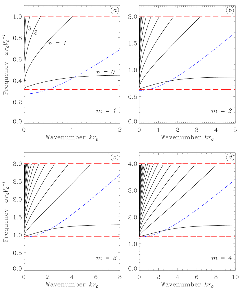
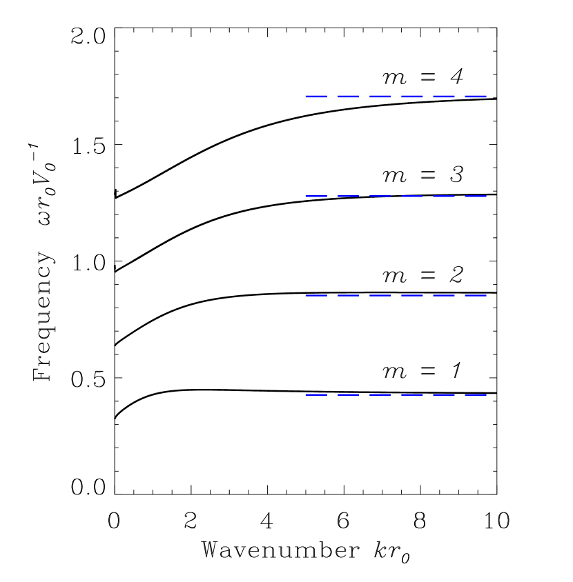
Since the dispersion relation is transcendental, we must solve it numerically if we wish to calculate the mode frequencies as a function of axial wavenumber and azimuthal order . We use the numerical codes developed by Gil et al. (2004) to numerically compute the Bessel functions of imaginary order and Press et al. (2007) to evaluate the Bessel functions. Figure 4 illustrates dispersion curves for the fundamental mode () and the first few azimuthal overtones (). Naturally, the solutions possess an integer number of nodes with radius, and the number of nodes (or the radial order ) labels each family of solutions. Each curve in Figure 4 corresponds to a mode of specific radial order, , but different axial wavenumber , which is of course continuous. Note, as a function of , each modal curve begins near the cut-off frequency of the outer shell. The radial overtones continue to increase with wavenumber until they disappear as they cross the high-frequency limit demarking recessive behavior at the origin. The gravest mode (), on the other hand, rapidly flattens as increases and asymptotes to a fixed value.
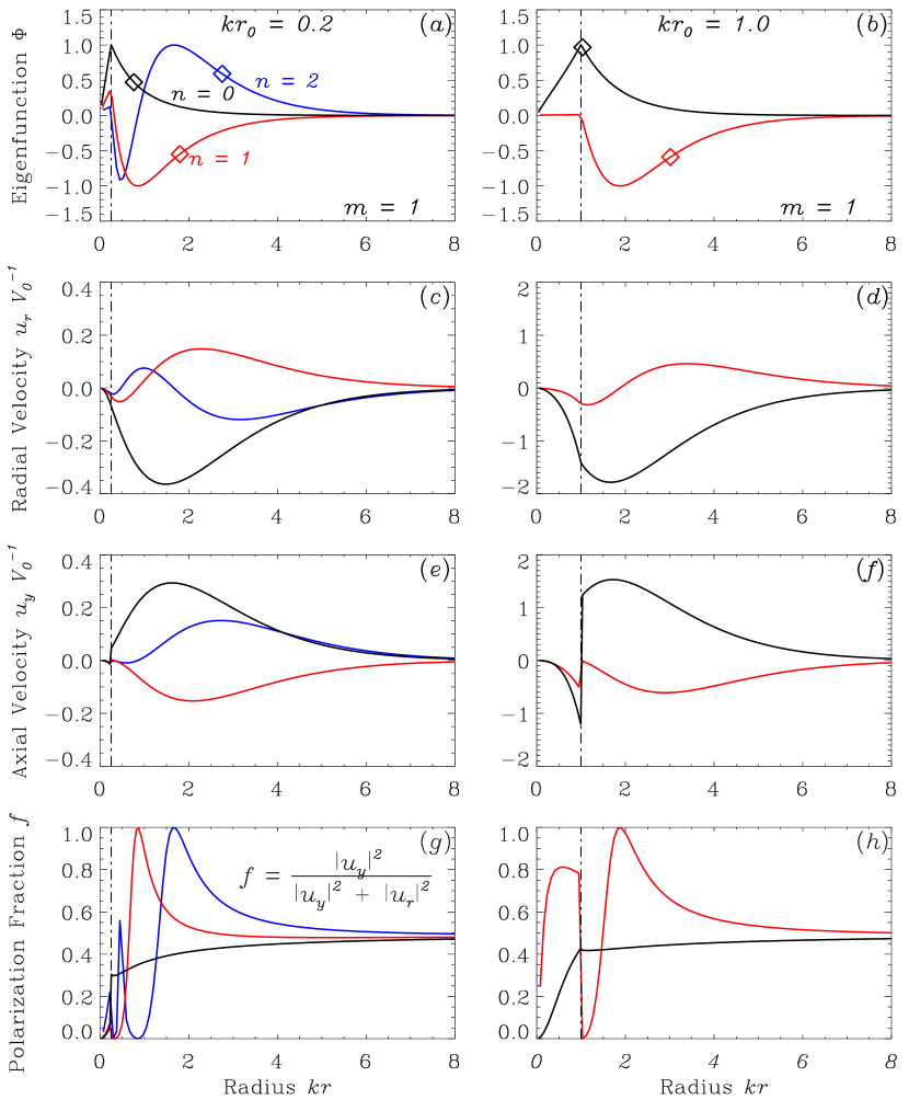
Figures 5– present radial eigenfunctions for the dimensionless-pressure fluctuation (Figures 5 and ), the radial velocity ( and ), and the axial velocity ( and ). All of the eigenfunctions are only for , although the higher azimuthal orders have similar behavior. The normalization constant in equation (4.34) has been chosen purely for illustrative purposes. Each of the panels corresponding to an axial wavenumber of show the gravest three radial orders. While for , only the eigenfunctions for and are shown, because does not exist. The matching conditions ensure that and are continuous across the interface between the two shells. The axial velocity is discontinuous and in fact changes sign across the interface.
In the inner shell, the eigenfunctions correspond to evanescent solutions that vanish at the origin. Within the outer shell, the solution may be propagating just above the interface and evanescent higher (if a body wave) or it may be evanescent throughout (if a surface wave). The lower boundary of the waveguide is the same for all modes and it is located at the interface between inner and outer shells. For the body waves, the upper boundary of the waveguide is different for each mode and corresponds to the turning point located at . Therefore, the radial size of the waveguide depends on frequency , axial wavenumber , and azimuthal order (because depends on ). These turning points are indicated in Figures 5 and by the colored diamonds. Note that the turning points should not correspond to the inflection points of . Instead, they are located at the inflection points of .
The gravest radial mode () is slightly unusual. At low axial wavenumber, the wave is a body wave with a narrow zone of propagation just above the interface. As the wavenumber increases, the mode changes into a surface wave that is evanescent everywhere. Since this mode only lives on the interface, its behavior is quite distinct from the higher overtones, and hence its dispersion relation does not follow the same pattern as the radial overtones.
5 Discussion
We have developed general equations describing the fast MHD eigenmodes of a coronal magnetic arcade possessing cylindrical geometry and an Alfvén speed that is a function of only the cylindrical radius, . We find that a waveguide exists as long as the Alfvén speed monotonically increases beyond some radius. This waveguide traps waves radially and azimuthally, and allows free propagation of the waves down the cylindrical axis. Thus, the eigenfunctions of the magnetic arcade consist of standing waves in radius and azimuth and traveling waves in the axial direction. We subsequently derived the eigenfunctions and eigenfrequencies for an arcade model with a specific Alfvén speed profile. In this model, the arcade has a diffuse, evacuated cavity that extends to a cylindrical radius of . The edge of the cavity consists of a density discontinuity over which hangs a shell of denser fluid. Separately in each region, the Alfvén speed is linearly proportional to the radius. Fast MHD waves can be trapped as body waves that live in the denser region above the density discontinuity at or as surface waves that reside on the density discontinuity itself.
We reiterate that the resonant oscillations of the arcade have both magnetic pressure and tension as restoring forces. This can be visually verified by noting in Figure 5 that the dimensionless magnetic pressure, , is always comparable in magnitude to the velocity components, which are themselves proportional to the magnetic tension. Only waves with zero axial wavenumber can be pure tension waves. This is a very different result from what is predicted by 1-D models that treat the loop as a single coherent entity. Those studies argue that the oscillations are fast MHD kink waves primarily driven by tension forces.
5.1 Observational Implications
Occasionally, the arcade itself may not be fully visible and only one or two preferentially illuminated loops can be seen. In such cases, fast MHD waves may be traversing the entire arcade but the 3-D wave field can only be sampled along a given field line. Since the wave modes of the arcade are trapped, standing waves in the direction parallel to the field (i.e., reflection from the two photospheric foot points), the motion of any individual field line may look very reminiscent of a 1-D wave cavity. Only by careful examination of the spectral content of the oscillations can the existence of the full 3-D wave field be surmised.
If the wave excitation region is sufficiently broad, we anticipate that the lowest-order modes in both radius and azimuth will be preferentially excited. Thus the surface wave is of particular importance. Furthermore, we expect that most of the emission, which is visible as a bright loop, should arise from the densest fluid. Hence, the cavity should be dim and the bright loop probably corresponds to only the narrow portion of the waveguide immediately above the interface at . If such a supposition is correct, the radial shear that appears in the axial velocity may not be evident. Further, even the radial overtones, which have nodes in radius, may appear as a single collimated oscillating loop.
Finally, we emphasize that each radial order actually comprises a continuum of eigenmodes with different axial wavenumbers . The relative amplitude of these modes will depend explicitly on the manner in which the waves are excited. However, in driven problems the mode with the lowest frequency is usually the most easily excited. From the dispersion curves, Figure 4, one would therefore expect that those modes with would dominate the spectrum, forming a distinct peak. Modes with nonzero wavenumber have higher frequency and thus would contribute power exclusively to the high-frequency wing of the peak. The resulting power spectrum would possess an asymmetric power peak with a deficit of power in the low-frequency wing. Scattering processes certainly broaden a spectral peak, but they typically do so symmetrically. Therefore, the existence of asymmetric power—as observed by Jain et al. (2015)—may be evidence for transverse wave propagation within a waveguide.
The surface wave could very well appear in power spectra with a doubly peaked profile. One peak would appear near the lowest frequency available, associated with the waves with . The second, higher-frequency peak would correspond to an accumulation of power from all of the modes with where the dispersion curve becomes flat. The width of each peak and relative amplitude would of course depend on the details of the driving.
5.2 Velocity Polarization
Coronal loops are observed to oscillate in two polarizations of motion. “Horizontal” oscillations involve swaying of the loops back and forth and correspond to axial motions in the geometry presented here. “Vertical” oscillations (Wang & Solanki, 2004) cause an expansion and contraction of the loop in radius and in our geometry such motions would be purely in the radial direction. For many of the observed loops, only one polarization is actually observable due to projection effects and the vantage of observation. Hence, one should be mindful that observations of a particular polarization are only proof that one of the possible polarizations exists, not as evidence that the other polarization is absent.
The arcade modes presented here never oscillate in a pure polarization, nor do all of the field lines passing through the waveguide oscillate as a coherent bundle. Instead, the cross-sectional shape of a sheaf of field lines shears and distorts during a period of the oscillation. Equations (3.8) and (3.9) reveal that the two polarizations are coupled in the 3-D arcade. The eigenfunctions illustrated in Figure 5 demonstrate the coupling by clearly showing that over most of the parameter regime, the two velocity components have similar magnitudes. From equations (3.8) and (3.9), we can immediately deduce that the axial and radial motions are 90∘ out of phase. Thus, the polarization is actually elliptical and any given parcel of fluid undergoes elliptical motion in the plane perpendicular to the local field line. The orientation of the minor and major axes is always the same (axial and radial), but the ellipticity depends explicitly on the polarization fraction, . This polarization fraction is presented in Figures 5 and for the same eigenfunctions that we provided earlier. A value of 1 corresponds to pure axial or horizontal motion and a polarization fraction of 0 indicates pure radial motion or vertical polarization. A polarization fraction of 0.5 indicates circular polarization.
Even the fundamental mode in radius, , which has the simplest radial behavior, changes polarizations as a function of height. Near the origin, where the mode has very weak motions, the polarization is primarily radial (or vertical). Throughout the inner cavity, the polarization shifts until it reaches an even admixture of the two polarizations within the outer shell (i.e., the polarization is nearly circular). For higher-order radial modes, the polarization swings back and forth between primarily axial (horizontal) to primarily radial (vertical), as one passes through the nodes of the respective eigenfunctions. Above the turning point, in the evanescent region of the eigenfunction, the polarization becomes nearly circular. However, since we do not expect the entire waveguide to be visible, the observed motion of a bright coronal loop is likely to possess a single polarization corresponding to the portion of the eigenfunction that lies directly above the interface at . If the fundamental radial mode is observed, this polarization should be nearly circular (see Figure 5), but if higher radial orders are observed, the polarization could be predominately radial.
5.3 Radial Shear in the Axial Velocity
The interface between the diffuse interior cavity and the outer shell of dense fluid is a region of intense shear. While the magnetic pressure and radial velocity are continuous across this layer, the axial velocity changes sign across the interface. Therefore, even for modes of the lowest radial order, the horizontal motion within the cavity is in the opposite direction compared to the motions in the overlying fluid. As stated previously, we suspect that much of this shear may remain invisible in a real arcade, as the emission generating the image of the bright loop likely arises from the dense fluid within the outer shell above the shear zone.
Since the interface between the cavity and outer shell is both a region of sharp increase in the mass density with radius and a zone of strong shear in the horizontal flow speed, this interface is ripe for the operation of the Kelvin-Helmholtz instability. Since the magnetic field points in a direction perpendicular to the shear, the instability is largely unaffected by the presence of the field. The linear growth rate arising from just the velocity shear (ignoring the effects of an unstable density gradient) is given by
| (5.37) |
where is the difference in the axial velocity across the interface at . To estimate a typical value for this growth rate, we use a transverse loop velocity of 100 m s-1 (Jain et al., 2015) and adopt a velocity jump of twice this value. If we assume that the density increases roughly by a factor of four across the interface, as is typical for a prominence cavity (Schmit & Gibson, 2011), the ratio of square Alfvén speeds has the same value. Thus, we estimate the growth rate to be m s-1. A ratio of this number to the local Alfvén speed should be constructed to determine the magnitude of the growth rate compared to a fast wave frequency. Given an Alfvén speed of 2000 km s-1. We estimate that the ratio of the growth rate to wave frequency is on the order of . Therefore, the growth rate is likely to be quite weak and any turbulent flows arising from the shear in the eigenfunctions are also likely to be small perturbations.
5.4 Surface Waves
Since the modes of lowest radial and azimuthal order are more efficiently excited by large-scale disturbances, we expect the mode to predominate. For low axial wavenumber this mode is a body wave. For large the mode transitions to a pure surface wave. In either case, the magnetic pressure fluctuation and the radial velocity have single lobed eigenfunctions. The magnetic pressure peaks at the interface at and the radial velocity peaks rather higher. The axial velocity is discontinuous at the interface and changes sign across it, but otherwise lacks zeros.
The dispersion relation for the fundamental radial mode is rather different from that of the overtones. First, the mode exists for all wavenumbers. This occurs because the eigenfrequency does not continue to rise as the wavenumber increases and thus does not disappear as it crosses over the upper frequency limit. In fact, the dispersion curve for the surface wave asymptotes to a finite value as the wavenumber increases to infinity. Figure 6 illustrates the behavior of the dispersion curves for . The curve corresponding to demonstrates that the approach to the asymptotic value is not always monotonic.
A quick asymptotic analysis of equation (4.22) for large axial wavenumbers confirms the results achieved by numerical evaluation of the full solution, namely, that for the two-shell model the surface wave has a frequency that becomes independent of , approaching a constant value that depends on the wavenumber parallel to the field lines and to the fractional change in the Alfvén speed across the interface ,
| (5.38) |
This asymptotic limit is indicated in Figure 6 by the horizontal dashed lines. We note that this dispersion relation is identical to that achieved for surface waves residing on the interface between two uniform media in Cartesian geometry when the transverse wavenumber is large (see Wentzel, 1979). This is a strong indication that in this limit, the surface wave becomes insensitive to the curvature of the field lines and to the stratification on either side of the interface. The lack of dependence on the stratification is expected because the mode becomes ever more confined to the interface as the axial wavenumber increases (i.e., the mode’s skin depth to either side shrinks). The lack of the dependence on the curvature may be a special property of the potential magnetic equilibrium. Note that there is an absence of curvature terms appearing in the momentum equation (3.5). Such terms would appear as a radial component of the tension proportional to . In the derivation of equation (3.5), all such terms were cancelled by corresponding terms appearing in the magnetic pressure force that arise from the radial variation of the magnetic field strength.
References
- Andries et al. (2009) Andries, J., Van Doorsselaere, T., Roberts, B., Verth, G., Verwichte, E., & Erdélyi, R. 2009, Space Sci. Rev., 149, 3
- Aschwanden et al. (1999) Aschwanden M. J., Fletcher, L., Schrijver, C. J., & Alexander, D. 1999, ApJ, 520, 880
- De Moortel & Brady (2007) De Moortel, I. & Brady, C.S. 2007, ApJ, 664, 1210
- Dunster (1990) Dunster, T.M. 1990, SIAM J. Math. Anal., 21, 995
- Gil et al. (2004) Gil, A., Segura, J., Temme, N.M. 2004, ACM Transactions on Mathematical Software, 30, 159
- Hindman & Jain (2014) Hindman, B. W. & Jain, R. 2014, ApJ, 784, 103
- Jain et al. (2015) Jain, R., Maurya, R.A., Hindman, B. W. 2015, ApJ, 804, L19
- Nakariakov et al. (1999) Nakariakov, V., Ofman, L., DeLuca, E., Roberts, B., & Davila, J. M. 1999, Science, 285, 862
- Press et al. (2007) Press, W.H., Teukolsky, S.A., Vetterling, W.T., & Flannery, B.P., 2007, Numerical Recipes: The Art of Scientific Computing, Third Edition, (Cambridge Univ. Press: Cambridge), ISBN-10: 0521880688.
- Roberts et al. (1984) Roberts, B., Edwin, P. M., & Benz, A. O. 1984, ApJ, 279, 857
- Schmit & Gibson (2011) Schmit, D.J. & Gibson, S.E. 2011, ApJ, 733, 1
- Van Doorsselaere et al. (2007) Van Doorsselaere, T., Nakariakov, V.M., & Verwichte, E. 2007, A&A, 473, 959
- Verwichte et al. (2009) Verwichte, E., Aschwanden, M. J., Van Doorsselaere, T., Foullon, C., & Nakariakov, V. M. 2009, ApJ, 698, 397
- Verwichte et al. (2004) Verwichte, E., Nakariakov, V. M., Ofman, L., & Deluca, E. E. 2004, Sol. Phys., 223, 77
- Wang & Solanki (2004) Wang, T. & Solanki, S. 2004, Å, 421, L33
- Wentzel (1979) Wentzel, D.G. 1979, ApJ, 227, 319