Eclipse observations of high-frequency oscillations in active region coronal loops

One of the mechanisms proposed for heating the corona above solar active regions is the damping of magnetohydrodynamic (MHD) waves. Continuing on previous work, we provide observational evidence for the existence of high-frequency MHD waves in coronal loops observed during the August 1999 total solar eclipse. A wavelet analysis is used to identify twenty $4\times 4$ arcsec² areas showing intensity oscillations. All detections lie in the frequency range 0.2–0.3 Hz (5–3 s), last for at least 3 periods at a confidence level of more than 99% and arise just outside known coronal loops. This leads us to suggest that they occur in low emission-measure or different temperature loops associated with the active region.

1 Introduction

The coronal heating mechanism is the subject of a great deal of debate. With a temperature of more than a million degrees, the corona is several orders of magnitude hotter than the photosphere and chromosphere, thus ruling out the possibility of heating via thermal conduction. Popular theories which attempt to explain coronal heating can be broadly grouped into two categories (see the review article by Priest & Schrijver 1999). One possibility is that a large number of magnetic reconnections, followed by current dissipation, result in frequent micro- or nano-flare activity (Parker 1988). The other theory argues that the heating is dominated by the damping of magnetohydrodynamic (MHD) waves – either propagating from the lower solar atmosphere or induced in active regions by reconnection – through ion viscosity and electrical resistivity (first introduced by Hollweg 1981). MHD waves have two very distinct extremes: magnetoacoustic (divided into slow and fast mode) and ‘pure’ Alfvén (divided into compressional and non-compressional) waves. Magnetoacoustic waves cause pressure variations in the coronal plasma as they propagate. By contrast, Alfvén waves will either be transverse and non-compressional, propagating parallel to the magnetic field, or compressional and modifying the magnetic flux density perpendicular to the field. The differences between the two main categories of waves are expected to be observable, since Alfvén waves cause only Doppler shifts in observed lines, whereas the magnetoacoustic waves are expected to cause intensity variations as well. The latter should be more readily observable since the intensity normally varies with the square of the electron density.

In the past, a number of authors have reported intensity, velocity and line width fluctuations in the corona. Koutchmy et al. (1983) used coronagraph observations to find evidence of fluctuation in the velocity measurements of the coronal line of Fe xiv at 5303 Å with periods of 300s, 80s and 43s. Their observations were limited by sky fluctuations, which led to their suggestion of using satellite telescopes or observations during solar total eclipse. Furthermore Pasachoff & Landman (1984), using observations made during a total eclipse, detected intensity fluctuations with frequencies in the range 0.5–2.0 Hz (periods of 0.5–2.0 s). Since then, more detections of possible MHD oscillations have been published and Aschwanden et al. (1999) produced a catalogue of all detected periodicities across the spectrum from 0.01 to 1000 s. Subsequently, a number of authors have reported further detections of coronal oscillations. Singh et al. (1997) observed fast magnetosonic disturbances with frequencies of 0.2 Hz during the 1995 total solar eclipse. Cowsiket et al. (1999) applied similar techniques to detect oscillations with frequencies in the range of 10-20 mHz during the 1998 total solar eclipse, while Sakurai et al. (2002) used spectroscopic data to detect Doppler velocity with a frequency of $\sim$57 mHz. More recently, total eclipse observations were published by Pasachoff et al. (2002), who found some evidence for waves with frequencies in the range of 0.75-1.0 Hz.

Porter et al. (1994a, b) have used numerical methods to simulate the damping of energy from slow- and fast-mode MHD waves. They concluded that slow-mode waves can deposit enough energy to heat the corona under certain conditions, and for periodicities $\tau\leq$100 s; for fast-mode waves the upper limit to periodicities is $\sim$1 s. In a bid to detect such high-frequency oscillations, Phillips et al. (2000, hereafter P00) developed the Solar Eclipse Coronal Imaging System (SECIS), an instrument capable of making high-cadence observations of solar eclipses. Williams et al. (2001, 2002, hereafter W01 and W02 respectively) reported SECIS detections of oscillations with frequencies around 0.1 Hz, which might provide enough energy to heat the corona efficiently. Here we report further instances of such high-frequency oscillations in the data as those presented by W01 and W02.

2 Data analysis & Results

2.1 Observations

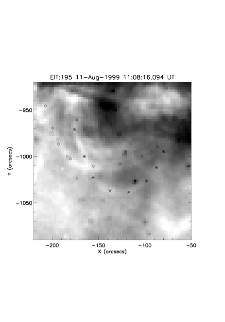
Figure 1: Marked with diamonds and asterisks are the two coronal loops in active region NOAA AR 8651 as observed by EIT in Fe xii (195 Å) formed at around 1.5 MK. The image is rotated clockwise by 123 deg to coincide with the orientation of the SECIS data. Both loops were also observed by SECIS and analysed for coronal oscillations.

Observations of the solar corona in Fe xiv 5303 Å (formed at $\sim$2.0 $\times$10⁶ K during the August 1999 eclipse were taken using the SECIS instrument (for a detailed description of the instrument see P00 and W01), with a sampling rate of 44 frames per second. The field of view of the instrument was $0.5\times 0.5$ deg² with a pixel size 4.0 arcsec pixel^-1. To increase the signal-to-noise, for each pixel the intensities of the eight adjacent pixels were added to it; i.e. as in W01 and W02 we have summed over a 3$\times$3 pixel² area. Two active region loops in NOAA AR 8651, observed both by the Solar and Heliospheric Observatory (SoHO) and through an Fe xiv (5303 Å) filter by SECIS, are highlighted in Fig. 1. Both loops were chosen as they are among the most well isolated in this active region and can clearly be seen in data from both SECIS and the EUV Imaging Telescope (EIT) on board SoHO. The latter observations were used to confirm the positions of these loops using several reference features.

2.2 Wavelet analysis

As in W01 and W02, we chose to analyse the data using a continuous wavelet analysis (for further details on this technique see Torrence & Compo 1998, hereafter TC98). Although Fourier analysis is overall more widely used, wavelet analysis has recently gained popularity, due to its ability to detect oscillations localised both in time and frequency. If an oscillation only lasts for a small fraction of the time series duration, Fourier analysis will be unable to detect it, whereas wavelet analysis is sensitive to even transient oscillatory signals. As the oscillations we hope to detect are relatively short (of the order of a few seconds) and our data extend over a period of around 40 s, wavelet analysis is ideal. Other authors (e.g. Gallagher et al. 1999; Ireland et al. 1999; Banerjee et al. 2000) have applied the same technique to detecting solar coronal oscillations. Additionally, the wavelet technique has consistently been used by W01 and W02, and a comparison with the results from these publications may help to draw interesting conclusions.

A Morlet wavelet was used for the analysis of our data, with

$$\psi(\eta)=\pi^{-1/4}\exp(i\omega_{0}\eta)\exp(\frac{-\eta^{2}}{2}),$$ (1)

where $\eta=t/s$ is the dimensionless time parameter, $t$ is the time, $s$ the scale of the wavelet (i.e. its duration), $\omega_{0}=s\omega$ is the dimensionless frequency parameter, and $\pi^{-1/4}$ is a normalization term (see TC98).

2.3 Detections

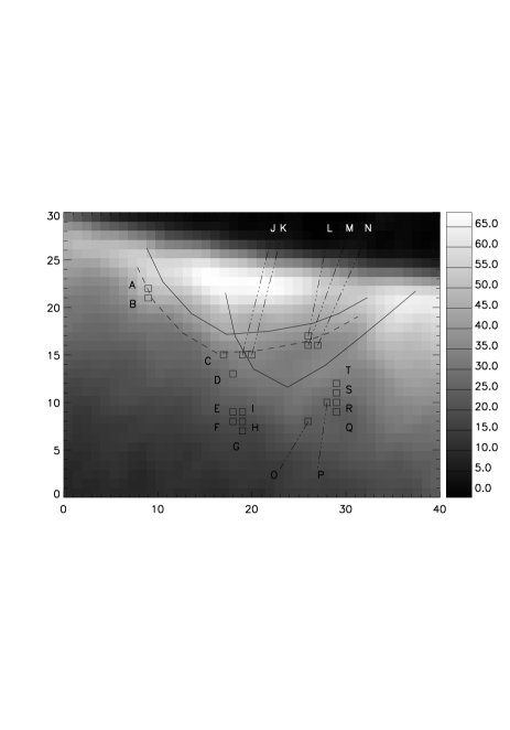
Figure 2: NOAA AR 8651 loops as observed by SECIS. The gray scale on the right-hand side corresponds to pixel counts. Only the tops of the loops shown in Fig. 1 are visible. The two solid lines highlight the two loops, while the squares contain pixels that show oscillations lasting three periods or longer. The 20 regions showing oscillations are labelled A to T. The dashed line is the solid line shifted by one pixel to the left and two pixels to the bottom, illustrating the good match of the shift to the pixels showing intensity oscillations.

Fig. 2 contains a time integrated (40 s) SECIS image of approximately the same region as Fig. 1. Since the lower parts of the corona are covered by the Moon, only the apexes of the loops identified in EIT Fe xii (195 Å) are observed by SECIS. The solid lines indicate the positions of the loops marked in Fig. 1 and the pixels marked with squares the areas that show intensity oscillation lasting three periods or longer. All twenty regions containing detected oscillations are labelled from A to T. Importantly, all the detections were made outside both bright loops toward the side where the corona is more tenuous. Although the areas of the corona that appear to host intensity oscillations are outside the visible loops, this has not led us to believe that these waves perturb outside coronal loops. It could simply be that the loops they travel through are low emission-measure structures that are too faint to be visible above the background. Furthermore, one may observe that in the case of the left-hand loop, the detections exactly coincide with a shift of the line which highlights the loop by one pixel to the left and two pixels down. The dashed line of Fig. 2 illustrates the close correlation between the shifted line of the loop and the pixels that have been detected with long intensity oscillations. Also, phase analysis of points A–T reveals no correlation between the phase of the oscillations detected in each point in space or time. This leads us to believe that this is not a simple case of a standing or travelling wave.

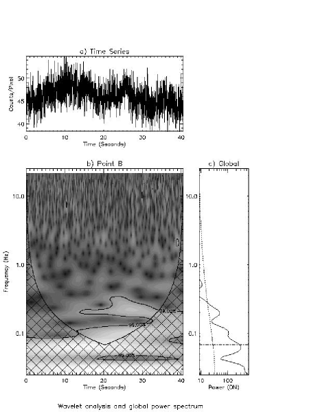
Figure 3: Wavelet transform analysis for point B in Fig. 2. (a) is the time series of the Fe xiv (5303 Å) line observations, (b) contains the wavelet transform of the time series and (c) the global wavelet spectrum. The brighter an area in (b), the greater the oscillatory power at the given time and frequency. The contours in this panel highlight the areas where the detected power is at the 99% confidence level. The hatched area of (b) represents the cone-of-influence (COI) and any detected oscillations within this region should be discarded as they might be influenced by edge effects. The scale of the frequency axis is logarithmic, while the time axis is linear and coincides with the time axis of (a). The dot-dashed line in (c) is a mark of the lowest limit of the COI and the dashed line the 99% significance level (as the contours of panel (b)). Both the power and frequency axes of (c) are logarithmic.

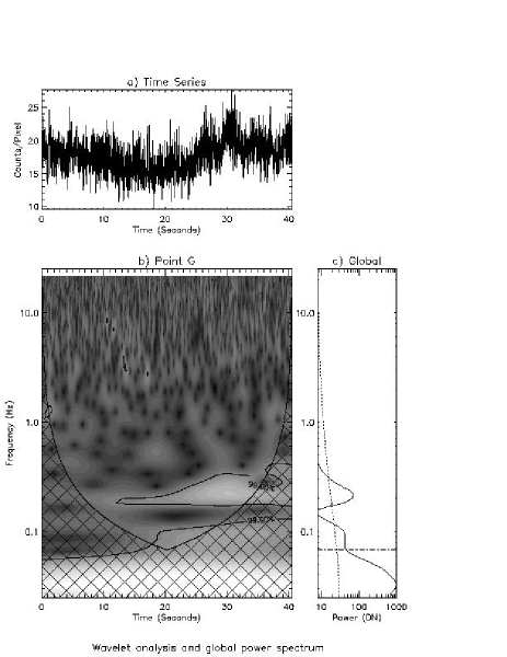
Figure 4: The wavelet analysis of point G in Fig. 2. For more details see caption of Fig. 3

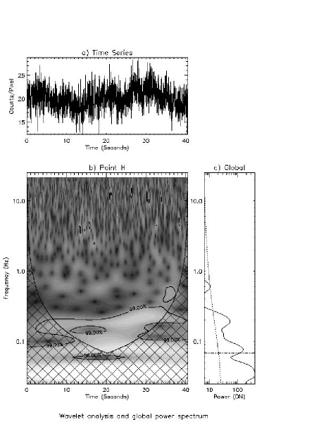
Figure 5: The wavelet analysis of point H in Fig. 2. For more details see caption of Fig. 3

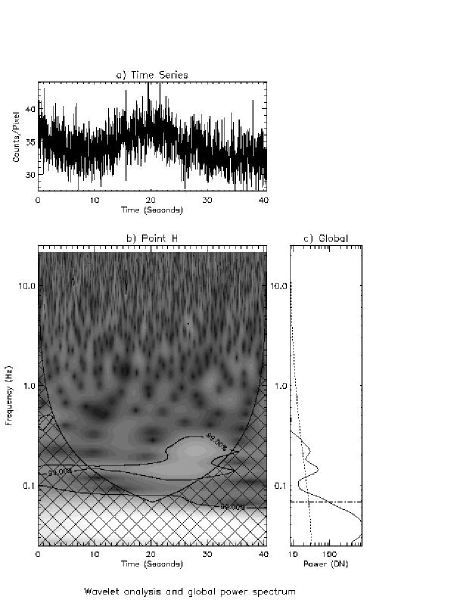
Figure 6: The wavelet analysis of point N in Fig. 2. For more details see caption of Fig. 3

Figs. 3–6 contain the results of the wavelet transform of a sample of points A to T in Fig. 2. The remaining figures are available from the first author upon request. Each figure is divided into three sections. Part (a) shows the time series generated by the Fe xiv (5303 Å) line filter (for details about the filter and the data reduction see W01). Part (b) is the power density wavelet transform of the time series in (a) : the brighter an area, the greater the power at the given time and frequency. The vertical axis is logarithmically scaled in frequency space while the horizontal axis is time on a linear scale. The time axis in (b) exactly coincides with that of the time series in (a), with the hatched region of (b) marking the cone-of-influence (COI). Everything inside the COI should be treated with suspicion, since any detections in this area may be influenced by edge effects in the wavelet transform calculation. For example a detection of a 0.5 Hz oscillation 0.5 s before the end of the time series is unreliable as there is not sufficient time for the oscillation in the wavelet packet to finish. For a more detailed discussion of the problem see TC98. The contours of panel (b) indicate where detected power exceeds the 99% confidence level, i.e., there is a 1% chance of the detection being due to Poisson noise.

Panel (c) contains the global wavelet spectrum, which is the wavelet analogue of the standard Fourier transform. It is produced by summing the power density wavelet transform over the whole time series, while the dotted line running along the frequency axis is the global significance level (again summed over time) at the same value (99%) as the contours in panel (b). The horizontal dot-dashed line near the bottom of panel (c) marks the bottom of the COI and all detections below this frequency should be discarded. Since the third panel provides no time information for the detections, the rest of the COI cannot be defined.

At this point it should be emphasized that there are two additional basic differences between panel (c) and the ‘traditional’ Fourier transform. Firstly, the spectrum is much smoother than the discrete Fourier power spectrum. Secondly, due to the wavelet transform’s use of ‘Heisenberg boxes’ (Mallat 1998), the better defined the transform is in time, the less well defined it will be in frequency.

Table 1 contains all the frequencies detected in each of the points from A to T. The length of these oscillations is also included in units of periodicities (i.e., a duration of three means that this particular oscillation lasted for three oscillatory periods at this frequency).

Point	A	B	C	D	E	F	G	H	I	J	K	L	M	N	O	P	Q	R	S	T
Period (s)	5	5	5.5	5	4	5	4.5	5	5.5	4.5	5	6.5	6.5	7	6	5	5	5	6	4
Duration (no. of periods)	4	4	3	3	4	3	4	5	3	3	3	3.5	3.5	3	3	3	3	3	3	3

Table 1: Frequencies detected in each of the points A through T. The duration of these oscillations is also included in units of Morlet periodicities (i.e. a duration of three means that this particular oscillation lasted for three oscillatory periods at this frequency).

3 Discussion

Although W01 and W02 have published similar detections from SECIS observations, the present work is by far the largest number of detections published to date. All twenty points presented here (Table 1) have passed a number of selection criteria. These include those used by W01 and W02 and the most important are summarised below:

• The frequencies of the detections are distinct from known instrumental frequencies (see W01).

• The contours of panel (b) were chosen at a 99% confidence level. Only oscillations within those contours were considered.

• All the reported detections lasted for at least three periods, so as to rule out rapid increases or decreases in the signal. When the duration of the oscillations was calculated, any portion within the COI was discarded.

As with all high-cadence systems producing data analysed for oscillations, the introduction of instrumental frequencies and the effect of noise is always a concern. To address the first limitation, wavelet analysis was deployed for parts of the image covered by the moon’s disk and the very faint parts of the corona. Any non-localised instrumental variations in pixel intensity should have affected these areas as much as the pixels of the active region. With the exception of those instrumental frequencies that are already known and discussed by W01, no other frequencies were detected. The other well-know cause of false detections is noise. To limit the possibility of a false detection because of noise, we chose to ignore any detections with frequencies above 1 Hz. It is widely accepted (for example Starck & Murtagh (2002) and references therein), that Gaussian or Poisson noise only affects frequencies of the same order as the sampling rate of the time series. As the sampling rate of the SECIS 1999 observations was 44 frames per second, the reported frequencies should be fairly unaffected by Gaussian or Poisson noise (which includes types of noise such as the CCD readout).

The two coronal loops of AR 8651 analysed here show a significant number of oscillations. Although only twenty oscillations were detected lasting three periods or longer, several tens of wave signatures were found which last between two and three periods at a $>99$% confidence level. This number is much larger than that expected considering the previous work on SECIS data (W01 and W02). Moreover, all previous detections were from the interior of bright coronal loops, while all of our oscillations are detected in fainter loops within the same active region, toward the tenuous part of the corona. Both of the above peculiarities can be explained by introducing a different physical mechanism to that suggested in W02. Zaqarashvili & Roberts (2002, 2003) have suggested a swing wave-wave interaction mechanism which may cause energy transformation from fast magnetoacoustic waves propagating across a magnetic field to Alfvén waves propagating along the field. They argue that, for a given medium density and magnetic field, the energy of fast waves can be converted to Alfvén waves with a basic harmonic at half the wavelength of the fast-mode wave. The above mechanism (also called swing absorption) may provide a possible explanation for the intensity oscillations reported here. In this scenario, Alfvén waves created in the upper photosphere (as described by Zaqarashvili & Roberts 2002, 2003) propagate along magnetic field lines adjacent to the coronal loops in Figs. 1 and 2. In the case of the first loop (points A, B, C, J, K, L, M, N of Fig. 2), a magnetic field line was running almost parallel to the left bright loop of Fig. 1, producing the alignment highlighted in Fig. 2. The rest of the points with detected oscillations (D–I and O–T) belong to one or another of the magnetic field lines in the same active region.

Litwin & Rosner (1993) proposed a multi-thread model, where many tiny loops with different physical parameters but in steady state equilibrium are superimposed forming the observed coronal loop structures. Aschwanden et al. (2000) used this model to explain the nonuniform heating of coronal loops observed by the Transition Region And Coronal Explorer (TRACE). Several such small threads may form thinner and fainter loops outside the bright structures appearing on Fig. 1 and 2. As the above oscillations travel through low emission-measure loops, it is easier for us to detect more oscillations than through high emission-measure loops (such as those studied by W01 and W02). Therefore the conditions under which those MHD waves propagate along points A–T are significantly different from those of the oscillations reported by W01 and W02. In their case the emission from the propagating waves is much stronger and as they and travel through a large number of threads, they stand significantly above the background emission of the loop. This is more clearly seen in W02, where the event that caused the oscillations also cause them to propagate with the same phase, enabling W02 to calculate the velocity of the perturbation by the phase difference of the traveling wave across the loop. In contrast to those detections, the area outlined by points A–T contains a smaller amount of threads with lower emission-measure, therefore relatively weaker MHD oscillations can be detected. This is supported by the results of the phase analysis that reveal no correlation in the phase of the 20 points with detected oscillations. The mechanism that produced the weaker waves (compared to those reported by W01 and W02) is less likely to produce them with the same phase. As the single-phase MHD waves are relatively rare events in the solar corona, we would expect them to appear in more extreme conditions (such as the release of large amounts of energy at the foot points of the loops) while the propagation of weaker oscillations through a smaller number of threads is more likely to take place under phase mixing conditions.

Cooper et al. (2003) suggest a possible mechanism that explains in some detail the detection of intensity oscillations as a line-of-sight effect of entirely incompressible MHD waves. In this model, when observed at an angle $\theta$ to the direction of propagation, the wave-induced deformation in a coronal loop causes intensity variations. This is because the amount of optically thin emitting plasma along the line of sight changes as a function of time. Cooper et al. (2003) find that the observed amplitude of the intensity oscillation can vary as a function not only of the true intensity of the oscillation and the angle between the propagation direction and the line-of-sight, but also of the wavelength of the perturbation. Furthermore, the observed frequency also varies as a function of the angle $\theta$, meaning that the detected periods listed in Table 1 may simply be higher harmonics of the true values.

Using the Cooper et al. (2003) and Zaqarashvili & Roberts (2002) results we were able to provide a satisfactory explanation of how the detected incompressible MHD waves were created in the vicinity of an active region in the photosphere, transmitted through low emission-measure loops to the lower corona and then detected as intensity oscillations by our imaging system. The large number (comparing to previous work) of detections and the alignment of some of these can be explained as the low emission that comes from the tenuous plasma makes any intensity oscillations more apparent, since the oscillating material makes for a higher percentage of the detected intensity.