Bayesian Analysis of Multiple Harmonic Oscillations in the Solar Corona

Abstract

The detection of multiple mode harmonic kink oscillations in coronal loops enables to obtain information on coronal density stratification and magnetic field expansion using seismology inversion techniques. The inference is based on the measurement of the period ratio between the fundamental mode and the first overtone and theoretical results for the period ratio under the hypotheses of coronal density stratification and magnetic field expansion of the wave guide. We present a Bayesian analysis of multiple mode harmonic oscillations for the inversion of the density scale height and magnetic flux tube expansion, under each of the hypotheses. Then, the two models are compared using a Bayesian model comparison scheme to assess how plausible each one is, given our current state of knowledge.

1. Introduction

Observations of magnetohydrodynamic (MHD) oscillations in solar coronal loops indicate the simultaneous presence of multiple mode harmonics in the same structure (Verwichte et al., 2004; De Moortel & Brady, 2007; Van Doorsselaere et al., 2007; O’Shea et al., 2007; van Doorsselaere et al., 2009). Their potential use for the diagnostic of the plasma conditions in the corona has attracted considerable interest (see Andries et al., 2009, for a review). The idea was first put forward by Andries et al. (2005) and Goossens et al. (2006) who found that the ratio of the fundamental mode period to twice that of its first overtone in the longitudinal direction depends on the density structuring along magnetic field lines. It is equal to unity in longitudinally uniform and unbounded tubes, but is smaller than one when density stratification is present. Using observational measurements of period ratios, Andries et al. (2005) and Van Doorsselaere et al. (2007) obtained estimates for the coronal density scale height.

An alternative hypothesis was formulated by Verth & Erdélyi (2008) whereby the expansion of the magnetic loop produces a deviation from unity in the period ratio, increasing its value. The effect is relevant for obtaining accurate estimates of the density scale height using multiple mode period ratios (Verth & Erdélyi, 2008; Verth et al., 2008; Ruderman et al., 2008). Observational evidence for magnetic tube expansion has been reported by e.g., Klimchuk (2000) in soft X-ray loops observed with Yohkoh and by Watko & Klimchuk (2000) in non-flare and postflare loops observed with TRACE. Observations of period ratios larger than one have been reported by O’Shea et al. (2007) and De Moortel & Brady (2007).

Since then, period ratio studies have analyzed different models for the density structuring in coronal loops (McEwan et al., 2006, 2008), the influence of the elliptic shape of loops (Morton & Erdélyi, 2009), the twist of the magnetic field (Karami & Bahari, 2012), the effect of the environment (Orza et al., 2012), and the temporal expansion of loops (Ballai & Orza, 2012). Period ratios have also been analyzed for slow MHD modes (Macnamara & Roberts, 2010) and for sausage modes (Macnamara & Roberts, 2011) and their use has been suggested in the context of prominence seismology (Díaz et al., 2010; Arregui et al., 2012).

Figure 1.— (a) Posterior distributions for $\eta$, under the density stratification model, for two values of the period ratio. (b) Posterior distributions for the magnetic tube expansion, $\Gamma$, under the magnetic expansion model, for two values of the period ratio. The measured period ratio and the inferred median of the distribution, with uncertainties given at the 68% credible interval are: (a) $r=0.91\pm 0.04$, $\eta=1.26^{+0.65}_{-0.59}$; $r=0.79\pm 0.03$, $\eta=3.39^{+0.72}_{-0.64}$. (b) $r=1.07\pm 0.04$, $\Gamma=1.20^{+0.10}_{-0.12}$; $r=1.38\pm 0.04$, $\Gamma=1.87^{+0.07}_{-0.07}$. The improved errors on $r$ in the measurements of Verwichte et al. (2004) have been taken from Van Doorsselaere et al. (2007). Similar errors are assigned to the mean values in the measurements by De Moortel & Brady (2007).

The application of Bayesian analysis techniques to coronal seismology is in its infancy. A first attempt of parameter inference using damped loop oscillations was presented by Arregui & Asensio Ramos (2011). In this paper, we present the first application of Bayesian model comparison techniques to coronal seismology. We first perform Bayesian parameter inference for the coronal density scale height and the magnetic tube expansion, under the two hypotheses of density stratification and magnetic field divergence, using multiple mode oscillations. Then, we assess which one of the two hypotheses better explains the observations, for given values of the period ratio.

2. Theoretical Models

The deviation from unity for the ratio between the fundamental and the first overtone transverse kink oscillation periods has been attributed to two main physical effects. Each one constitutes a hypothesis to explain the data.

In the model by Andries et al. (2005) coronal density stratification produces a decrease of the period ratio. This model projects a vertically stratified isothermal atmosphere onto a semicircular loop. An analytical expression for the dependence of the period ratio on density scale height was obtained by Safari et al. (2007). This expression can be rewritten as

$$r_{1}=\frac{P_{1}}{2P_{2}}=1-\frac{4}{5}\left(\frac{\eta}{\eta+3\pi^{2}}\right),$$ (1)

with $P_{1}$ and $P_{2}$ the periods of the fundamental and first overtone modes, $\eta=L/\pi H$ the ratio of the loop height at the apex to the density scale height $H$, and $L$ the loop length. We have checked that Equation (1) provides us with a good approximation to the numerical results by Andries et al. (2005).

In the model by Verth & Erdélyi (2008) magnetic tube expansion produces an increase of the period ratio given by

$$r_{2}=\frac{P_{1}}{2P_{2}}=1+\frac{3(\Gamma^{2}-1)}{2\pi^{2}},$$ (2)

with the expansion defined as $\Gamma=r_{a}/r_{f}$, where $r_{a}$ is the radius at the apex and $r_{f}$ is the radius at the footpoint. Equation (2) was obtained under the assumption that $|\Gamma-1|\ll 1$. Moreover, it is the result for a particular expanding loop model. Another equilibrium state will produce a quantitatively different result, although Ruderman et al. (2008) anticipate a qualitatively similar result.

Both longitudinal stratification and magnetic tube expansion have forward models that relate one observed quantity, the period ratio $P_{1}/2P_{2}$, to one physical quantity to be inferred, $\eta$ or $\Gamma$.

3. Bayesian Parameter Inference

To perform the inference using existing estimates for the period ratio we employ Bayes’ theorem (Bayes & Price, 1763)

$$p(\mbox{{\boldmath$\theta$}}|D,M)=\frac{p(D|\mbox{{\boldmath$\theta$}},M)p(\mbox{{\boldmath$\theta$}}|M)}{\int d\mbox{{\boldmath$\theta$}}p(D|\mbox{{\boldmath$\theta$}},M)p(\mbox{{\boldmath$\theta$}}|M)},$$ (3)

which gives the solution to the inverse problem in terms of the posterior probability distribution, $p(\mbox{{\boldmath$\theta$}}|D,M)$, that describes how probability is distributed among the possible values of the unknown parameter, $\theta$, given the data $D$ and the assumed model $M$. The function $p(D|\mbox{{\boldmath$\theta$}},M)$ is the likelihood of obtaining a data realization actually observed as a function of the parameter vector and provides a measure of how well the data are predicted by the model. The prior probability $p(\mbox{{\boldmath$\theta$}}|M)$ encodes any prior information we might have on the model parameters, without taking into account the observed data. The denominator is the evidence, an integral of the likelihood over the prior distribution. This quantity plays no role in parameter inference, but will become central in the model comparison described in Section 4.

3.1. Longitudinally Stratified Loops

For longitudinally stratified loops, model $M_{1}$, the forward problem is given in Eq. (1). To evaluate the likelihood, we assume the model is true. Then, the period ratio measurement ($r$) will differ from the prediction ($r_{1}$) because of measurement uncertainties ($e$), so that $r=r_{1}\pm e$. The probability of obtaining the measured value is equal to the probability of the error. Assuming Gaussian errors, the likelihood for model $M_{1}$ is then expressed in the following manner

$$p(r|\eta,M_{1})=\frac{1}{\sqrt{2\pi}\sigma}\exp\left[-\frac{(r-r_{1})^{2}}{2\sigma^{2}}\right],$$ (4)

with $\sigma^{2}$ the variance associated to the observed period ratio. In the following we assign observed period ratio errors to the standard deviation $\sigma$.

The prior indicates our level of knowledge (ignorance) before considering the observed data. We have adopted a uniform prior distribution for the unknown, $\eta$, over a given range, so that we can write

$$p(\eta|M_{1})=\frac{1}{\eta^{\mathrm{max}}-\eta^{\mathrm{min}}}\mbox{\hskip 5.69046pt}\mbox{for}\mbox{\hskip 5.69046pt}\eta^{\mathrm{min}}\leq\eta\leq\eta^{\mathrm{max}},$$ (5)

and zero otherwise. We only consider loops with density decreasing with height. We know from observations that very large coronal loops with the apex height above several atmospheric scale heights exist, so we consider the range $\eta\in[0,8]$ in the prior above.

Parameter inference is next performed using Bayes’ theorem (3). We use period ratio measurements reported in observations by Verwichte et al. (2004). We must note that unambiguous identification of measured periods with particular overtones is a difficult task. Early observations were limited to the measurement of different periodicities at a single point, without spatial information (Verwichte et al., 2004). Even in the case in which information at different cuts along the loops is available (De Moortel & Brady, 2007), it is unclear how one should assign those periods to theoretical overtones. As our paper aims at providing a method to perform parameter inference and model comparison, we have considered period ratio values discussed in the review by Andries et al. (2009), noting that the reliability of the results is closely related to that of the adopted assumptions and theoretical interpretations.

Figure 1a shows posterior probability distributions for $\eta$ computed using Eq. (3) with likelihood and prior given by Eqs. (4) and (5), for two period ratio measurements by Verwichte et al. (2004). Well constrained distributions are obtained. For the measured period ratios $r\sim 0.79$ and $r\sim 0.91$, the inversion leads to density scale heights of $H=21$ Mm and $H=56$ Mm, respectively, for a loop with a height at the apex of $L/\pi=70$ Mm.

3.2. Expanding Magnetic Loops

For expanding loops, model $M_{2}$, the forward problem is given in Eq. (2). To evaluate the likelihood, we follow the same procedure as above, which leads to

$$p(r|\Gamma,M_{2})=\frac{1}{\sqrt{2\pi}\sigma}\exp\left[-\frac{(r-r_{2})^{2}}{2\sigma^{2}}\right].$$ (6)

We also adopt a uniform prior distribution for the unknown $\Gamma$, so that we can write

$$p(\Gamma|M_{2})=\frac{1}{\Gamma^{\mathrm{max}}-\Gamma^{\mathrm{min}}}\mbox{\hskip 5.69046pt}\mbox{for}\mbox{\hskip 5.69046pt}\Gamma^{\mathrm{min}}\leq\Gamma\leq\Gamma^{\mathrm{max}},$$ (7)

and zero otherwise. We consider $\Gamma\in[1,2.5]$.

Figure 1b shows posterior probability distributions for $\Gamma$ computed using Eq. (3) with likelihood and prior given by Eqs. (6) and (7), for two period ratio measurements. Again, well constrained distributions are obtained. Andries et al. (2009) discuss period ratio measurements in Table 1 by De Moortel & Brady (2007). Assuming that either the most power is in the fundamental mode or in the first overtone, mean values for the period ratio of $r\sim 1.07$ and $r\sim 1.38$ are obtained. For those values, the inversion leads to tube expansion factors that are compatible with the estimates by Klimchuk (2000) and Watko & Klimchuk (2000). Note however that, according to Fig 1b, a period ratio of $r\sim 1.38$ requires an expansion of the tube by a factor of $\Gamma\sim 1.85$, while observations by Watko & Klimchuk (2000) seem to indicate that in only very few cases does this parameter approach or exceed a value of $2$.

For both theoretical models, the Bayesian framework makes use of all the available information in a consistent manner and enables us to consistently propagate errors from observations to inferred parameters.

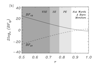
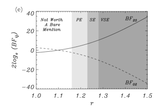
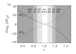
Figure 2.— (a) Marginal likelihoods computed using Eq. (11) for models $M_{0}$, $M_{1}$ and $M_{2}$ as a function of the data. (b)-(d) Bayes factors computed using Eq. (10) for the model comparisons between $M_{1}$ over $M_{0}$, $M_{2}$ over $M_{0}$, and $M_{1}$ over $M_{2}$. In (b)-(d), white regions indicate evidence not worth more than a bare mention (2 log${}_{e}BF\in[0,2]$); PE: positive evidence (2 log${}_{e}BF\in[2,6]$); SE: strong evidence (2 log${}_{e}BF\in[6,10]$);VSE: very strong evidence (2 log${}_{e}BF>10$). Uniform priors in the ranges $\eta\in[0,8]$ and $\Gamma\in[1,2.5]$ have been taken. In all figures $\sigma=0.08$.

4. Bayesian Model Comparison

Parameter inference was performed under the hypothesis that observed period ratios are the effect of either density stratification or magnetic tube expansion. The probability distributions in Figure 1 are conditional on the specific models used to explain the observations. The Bayesian framework enables us to present different models to the same data and assess in a quantitative manner which one is favored by them. We have compared three models: $M_{0}$ for a uniform density and magnetic field strength tube, $M_{1}$ for a longitudinally stratified loop, and $M_{2}$ for a expanding magnetic loop.

As model $M_{0}$ predicts a period ratio of one, regardless of $\eta$ or $\Gamma$, we can write

$$p(r|M_{0})=\frac{1}{\sqrt{2\pi}\sigma}\exp\left[-\frac{(r-1)^{2}}{2\sigma^{2}}\right],$$ (8)

for the likelihood in this case. Note that $p(r|M_{0})=p(r|\eta,M_{0})=p(r|\Gamma,M_{0})$.

To determine the plausibility of models $M_{1}$ and $M_{2}$ between them and with respect to model $M_{0}$, we evaluate the posterior probabilities to ascertain the relative merits of two models, $M_{i}$ and $M_{j}$. This is done by applying Bayes’ theorem (Eq. 3) to the two models and considering posterior ratios of the form (Jeffreys, 1961)

$$\frac{p(M_{i}|r)}{p(M_{j}|r)}=\frac{p(r|M_{i})}{p(r|M_{j})}\frac{p(M_{i})}{p(M_{j})}.$$ (9)

The first ratio on the right-hand side is the Bayes factor. It expresses how well the observed data are predicted by model $M_{i}$, compared to model $M_{j}$. The second ratio, the prior odds ratio, measures how much our initial beliefs favored $M_{i}$ over $M_{j}$, before considering the data. As we have no particular a priori preference for one model over the other, before considering the data, we take $p(M_{i})=p(M_{j})=1/2$. Our assessment of the plausibility of models is then based on the computation of the Bayes factor of $M_{i}$ against $M_{j}$ given by

$$BF_{ij}=\frac{p(r|M_{i})}{p(r|M_{j})}.$$ (10)

In model selection, we are interested in the most probable model, independently of the parameters, i.e., we should marginalise out all parameters. This is achieved by performing an integral of the likelihood over the full parameter space. The marginal likelihood for a given model $M_{i}$ is then

$$p(r|M_{i})=\int^{\theta^{\mathrm{m}ax}}_{\theta^{\mathrm{m}in}}p(r,\theta|M_{i})d\theta=\int^{\theta^{\mathrm{m}ax}}_{\theta^{\mathrm{m}in}}p(r|\theta,M_{i})p(\theta|M_{i})d\theta,$$ (11)

where $\theta\in[\theta^{\mathrm{m}in},\theta^{\mathrm{m}ax}]$ represents the particular parameter of the model and we have used the product rule to expand the probability of $r$ and $\theta$, given model $M_{i}$.

Figure 2a displays the marginal likelihoods for the three considered models. For a given observed period ratio, the plausibility of one model over the other is given by the ratio of these two quantities at the measured period ratio $r$. The uniform model has a marginal likelihood that is maximum at one. The model with density stratification is clearly favored for observations of period ratios below unity. Figure 2b quantifies the relative performance of models $M_{1}$ and $M_{0}$ by computing the Bayes factor. The lower $r$, the more plausible $M_{1}$ is against $M_{0}$. Jeffreys’ scale (Jeffreys, 1961; Kass & Raftery, 1995) assigns different levels of evidence to the values of the Bayes factor in natural logarithm units. They are shown using different darkening options in Figures 2b-d. According to Figure 2b, and given the assumed uncertainty of $\sigma=0.08$, a period ratio measurement should be considered as positive evidence for model $M_{1}$ against model $M_{0}$ only if it is below 0.87. As strong evidence, only if it is below 0.78. A period ratio below 0.71 indicates very strong evidence for model $M_{1}$.

A similar comparison was made for models $M_{2}$ and $M_{0}$ (Figure 2c). The model for magnetic tube expansion is clearly favored for observations of period ratios above unity. Model $M_{0}$ cannot be ruled out by the simple fact that $r>1$. Positive evidence for model $M_{2}$ against model $M_{0}$ exists for period ratio measurements above 1.16. If $r>1.23$, there is strong evidence for model $M_{2}$. A period ratio above 1.28 indicates very strong evidence for model $M_{2}$.

Finally, we have compared model $M_{1}$ against model $M_{2}$, in view of observed data. Figure 2d shows that the evidence is the same for both models if the period ratio is unity. Around this value, there is a region, $0.96<r<1.06$, in which no firm conclusion can be established. Positive, strong, and very strong evidence for $M_{1}$ occur below 0.96, 0.87, and 0.80, respectively. Positive, strong, and very strong evidence for $M_{2}$ occur above 1.06, 1.15, and 1.21, respectively.

In our model comparison, $\sigma=0.08$ has been selected so as to clearly show the different regimes for the evidence. An increase (decrease) of $\sigma$ produces a decrease (increase) of any evidence. The inference in Figure 1a for $r=0.91$ with uncertainty of $\sigma=0.04$ falls into the region of positive evidence for hypothesis $M_{1}$. The inference in Figure 1b for $r=1.07$ should have an uncertainty of $\sigma=0.03$ (close to the reported error) to be considered done under positive evidence for hypothesis $M_{2}$.

5. Conclusions

We have presented a simple and straightforward technique to perform parameter inference and model comparison using period ratios of kink oscillations in the Bayesian framework. Parameter inference enable us to obtain estimates for the coronal density scale height and the magnetic loop expansion, using all the available information and with correctly propagated uncertainties. Density scale height estimates are compatible with previous studies. Magnetic tube expansion factors are compatible with the estimates by Klimchuk (2000) and Watko & Klimchuk (2000). Even if Eqs. (1) and (2) imply well-posed inversion problems from a mathematical point of view, the unknown parameters cannot be obtained uniquely, due to the uncertainties associated to observed data. The Bayesian framework enables us to consistently deal with this problem.

Bayesian model comparison enable us to assess the plausibility of the inferences, which are conditional on theoretical models. Deviations of the period ratio below (above) unity do not necessarily imply density stratification (tube expansion) to be preferred in front of the null hypothesis. The degree of evidence for the two theories so far invoked can be quantitatively assessed with the use of Bayes factors, to precisely decide which one of the two hypotheses is more plausible, for a given measured period ratio and the associated uncertainty.

Our analysis provides a simple and easy to use method to perform inference and model comparison in the presence of incomplete and uncertain information. Measured period ratios and their uncertainties determine the strength of the evidence in favour of a particular hypothesis and, therefore, the support of the performed inferences.

The Bayesian formalism for inference and model comparison is the only fully correct way we have to get information about physical parameters and the plausibility of hypotheses from observations (see e.g. Trotta, 2008; von Toussaint, 2011) under incomplete and uncertain information. Arregui & Asensio Ramos (2011) performed the first Bayesian parameter inference in coronal seismology. This paper presents the first application of Bayesian techniques to model comparison. When analytical forward problems are available, both parameter inference and model comparison reduce to a simple and straightforward evaluation of the marginal posteriors and the Bayes factors, that can be obtained by solving simple integrals. The methods outlined in this paper can be directly applied to most of the seismology inversion problems in which other physical effects and parameters are involved. For instance, additional effects that influence period ratios could be compared to the already considered hypotheses.

References

- Andries et al. (2005) Andries, J., Arregui, I., & Goossens, M. 2005, ApJ, 624, L57
- Andries et al. (2009) Andries, J., van Doorsselaere, T., Roberts, B., Verth, G., Verwichte, E., & Erdélyi, R. 2009, Space Sci. Rev., 149, 3
- Arregui & Asensio Ramos (2011) Arregui, I., & Asensio Ramos, A. 2011, ApJ, 740, 44
- Arregui et al. (2012) Arregui, I., Oliver, R., & Ballester, J. L. 2012, Living Reviews in Solar Physics, 9, 2
- Ballai & Orza (2012) Ballai, I., & Orza, B. 2012, A&A, 545, A118
- Bayes & Price (1763) Bayes, M., & Price, M. 1763, Royal Society of London Philosophical Transactions Series I, 53, 370
- De Moortel & Brady (2007) De Moortel, I., & Brady, C. S. 2007, ApJ, 664, 1210
- Díaz et al. (2010) Díaz, A., Oliver, R., & Ballester, J. 2010, Astrophys. J., 725, 1742
- Goossens et al. (2006) Goossens, M., Andries, J., & Arregui, I. 2006, Royal Society of London Philosophical Transactions Series A, 364, 433
- Jeffreys (1961) Jeffreys, H. 1961, in Theory of Probability (3rd ed.) (Oxford University Press)
- Karami & Bahari (2012) Karami, K., & Bahari, K. 2012, ApJ, 757, 186
- Kass & Raftery (1995) Kass, R. E., & Raftery, A. E. 1995, JASA, 90, 773
- Klimchuk (2000) Klimchuk, J. A. 2000, Sol. Phys., 193, 53
- Macnamara & Roberts (2010) Macnamara, C. K., & Roberts, B. 2010, A&A, 515, A41
- Macnamara & Roberts (2011) —. 2011, A&A, 526, A75
- McEwan et al. (2008) McEwan, M. P., Díaz, A. J., & Roberts, B. 2008, A&A, 481, 819
- McEwan et al. (2006) McEwan, M. P., Donnelly, G. R., Díaz, A. J., & Roberts, B. 2006, A&A, 460, 893
- Morton & Erdélyi (2009) Morton, R. J., & Erdélyi, R. 2009, A&A, 502, 315
- Orza et al. (2012) Orza, B., Ballai, I., Jain, R., & Murawski, K. 2012, A&A, 537, A41
- O’Shea et al. (2007) O’Shea, E., Srivastava, A. K., Doyle, J. G., & Banerjee, D. 2007, A&A, 473, L13
- Ruderman et al. (2008) Ruderman, M. S., Verth, G., & Erdélyi, R. 2008, ApJ, 686, 694
- Safari et al. (2007) Safari, H., Nasiri, S., & Sobouti, Y. 2007, A&A, 470, 1111
- Trotta (2008) Trotta, R. 2008, Contemporary Physics, 49, 71
- van Doorsselaere et al. (2009) van Doorsselaere, T., Birtill, D. C. C., & Evans, G. R. 2009, A&A, 508, 1485
- Van Doorsselaere et al. (2007) Van Doorsselaere, T., Nakariakov, V. M., & Verwichte, E. 2007, A&A, 473, 959
- Verth & Erdélyi (2008) Verth, G., & Erdélyi, R. 2008, A&A, 486, 1015
- Verth et al. (2008) Verth, G., Erdélyi, R., & Jess, D. B. 2008, ApJ, 687, L45
- Verwichte et al. (2004) Verwichte, E., Nakariakov, V. M., Ofman, L., & Deluca, E. E. 2004, Sol. Phys., 223, 77
- von Toussaint (2011) von Toussaint, U. 2011, Reviews of Modern Physics, 83, 943
- Watko & Klimchuk (2000) Watko, J. A., & Klimchuk, J. A. 2000, Sol. Phys., 193, 77