Synthetic Emissions of the Fe XXI 1354 Å Line from Flare Loops Experiencing Fundamental Fast Sausage Oscillations

Abstract

Inspired by recent IRIS observations, we forward model the response of the Fe XXI 1354 Å line to fundamental, standing, linear fast sausage modes (FSMs) in flare loops. Starting with the fluid parameters for an FSM in a straight tube with equilibrium parameters largely compatible with the IRIS measurements, we synthesize the line profiles by incorporating the non-Equilibrium Ionization (NEI) effect in the computation of the contribution function. We find that both the intensity and Doppler shift oscillate at the wave period ($P$). The phase difference between the two differs from the expected value ($90^{\circ}$) only slightly because NEI plays only a marginal role in determining the ionic fraction of Fe XXI in the examined dense loop. The Doppler width modulations, however, posses an asymmetry in the first and second halves of a wave period, leading to a secondary periodicity at $P/2$ in addition to the primary one at $P$. This behavior results from the competition between the broadening due to bulk flow and that due to temperature variations, with the latter being stronger but not overwhelmingly so. These expected signatures, with the exception of the Doppler width, are largely consistent with the IRIS measurements, thereby corroborating the reported detection of a fundamental FSM. The forward modeled signatures are useful for identifying fundamental FSMs in flare loops from measurements of the Fe XXI 1354 Å line with instruments similar to IRIS, even though a much higher cadence is required for the expected behavior in the Doppler widths to be detected.

1 Introduction

Magnetohydrodynamic (MHD) waves and oscillations have been amply found in the highly structured solar corona (see recent reviews by e.g., Nakariakov & Verwichte, 2005; Banerjee et al., 2007; De Moortel & Nakariakov, 2012; Nakariakov et al., 2016). Theoretically, fast sausage modes (FSMs) are characterized by the absence of azimuthal dependence of the associated perturbations and also by their axial phase speeds being on the order of the Alfvén ones (e.g., Edwin & Roberts, 1983). FSMs can be either leaky or trapped depending on the longitudinal wavenumber $k$ (Cally 1986, also see e.g., Rosenberg 1970; Zajtsev & Stepanov 1975; Meerson et al. 1978; Terradas et al. 2005; and Kopylova et al. 2007). Considerable efforts have gone into examining how FSMs in coronal structures depend on the spatial distribution of the equilibrium parameters, thereby addressing such effects as the density distribution (e.g., Inglis et al., 2009; Nakariakov et al., 2012; Chen et al., 2015; Yu et al., 2015; Chen et al., 2016; Cally & Xiong, 2018), siphon flow (e.g., Terra-Homem et al., 2003; Li et al., 2013, 2014), and magnetic twist (e.g., Bennett et al., 1999; Erdélyi & Fedun, 2007; Khongorova et al., 2012). Observationally, FSMs are often invoked to interpret quasi-periodic pulsations (QPPs) with quasi-periods ranging from a few seconds to a couple of tens of seconds in solar flares (for recent reviews, see e.g., Nakariakov & Melnikov, 2009; Van Doorsselaere et al., 2016b; McLaughlin et al., 2018). For instance, the existence of fundamental standing FSMs in flare loops was inferred from the radio pulsations for a substantial number of flares measured by the Nobeyama Radioheliograph (e.g., Nakariakov et al., 2003; Melnikov et al., 2005; Kolotkov et al., 2015). Likewise, signatures of FSMs were also found in the fine structures in a number of flare-associated radio bursts as measured by, say, the Chinese Solar Broadband Radio Spectrometer (Yu et al., 2013, 2016), the Assembly of Metric-band Aperture Telescope and Real-time Analysis System (Kaneda et al., 2018), and the LOw Frequency ARray (Kolotkov et al., 2018). Furthermore, a recent multi-wavelength study by Nakariakov et al. (2018) suggested the existence of FSMs in loops associated with microflares. In extreme ultraviolet (EUV), Su et al. (2012) identified FSMs using imaging observations in the 171 Å channel of the Atmospheric Imaging Assembly (AIA) aboard the Solar Dynamics Observatory (SDO). Recently, the oscillatory behavior in the profile of the Fe XXI 1354 Å line as measured by the Interface Region Imaging Spectrograph (IRIS) was attributed to the fundamental standing FSM hosted by flare loops (Tian et al., 2016, hereafter T16).

Forward modeling plays an important role in the practice of wave mode identification, which is often not straightforward in the case of FSMs. Cooper et al. (2003) and Gruszecki et al. (2012) integrated the squared density along a line-of-sight (LoS) to compute the intensity modulations, thereby examining the effects of, say, instrumental resolutions on the detectability of FSMs in coronal loops. These effects on the synthetic profiles of the Fe IX 171 Å and Fe XII 193 Å lines were then examined, in a rather exhaustive manner, by Antolin & Van Doorsselaere (2013) who incorporated the relevant contribution functions. As found from this series of studies, the modulations in the intensities, Doppler shifts, and Doppler widths are detectable even when the pixel size (temporal cadence) is a substantial fraction of the axial wavelength (wave period). Still addressing the Fe IX 171 Å and Fe XII 193 Å lines, our recent study further examined how non-equilibrium ionization (NEI) affects the spectral signatures of FSMs in active region loops (Shi et al., 2019, hereafter paper I). It was found that NEI has little effect on the Doppler shift or width, but tends to substantially reduce the intensity modulations, making the detection of FSMs in tenuous loops possibly challenging.

This study aims to extend our paper I by forward modeling the spectral signatures of fundamental FSMs in flare loops for the Fe XXI 1354 Å line, as inspired by T16. Such a study has not appeared in the literature to our knowledge, and is expected to find applications for identifying FSMs with the rich information that this flare line can offer. This manuscript is organized as follows. In Section 2 we present the necessary expressions for the perturbations associated with linear FSMs, and describe the procedure for synthesizing the Fe XXI 1354 Å line profiles. The synthetic emission properties are then detailed in Section 3. Section 4 summarizes this study, ending with some concluding remarks.

2 Model Formulation

2.1 Fundamental Fast Sausage Modes In Flare Loops

We model an equilibrium flare loop as a static, straight cylinder with mean radius $R=5\times 10^{3}$ km and length $L=4.5\times 10^{4}$ km. In a cylindrical coordinate system ($r,\phi,z$), both the cylinder axis and the equilibrium magnetic field ${\mathbf{B}}$ are in the $z$-direction. We adopt single-fluid ideal MHD and consider an electron-proton plasma throughout. Gravity is neglected. We further assume that the equilibrium parameters depend only on $r$, and in such a way that the configuration comprises a uniform cord (denoted by subscript $\rm i$), a uniform external medium (subscript $\rm e$), and a transition layer (TL) continuously connecting the two. Let $N$, $T$, and $B$ denote the electron number density, electron temperature, and magnetic field strength, respectively. Furthermore, let subscript $0$ denote the equilibrium values. In the cord, we take $N_{\rm i}=5\times 10^{10}{\rm~{}cm}^{-3}$, $T_{\rm i}=10~{}{\rm MK}$, and $B_{\rm i}=43~{}{\rm G}$, resulting in an internal Alfvén speed $v_{\rm Ai}$ of $420~{}{\rm km}~{}{\rm s}^{-1}$. We assume that $N_{0}$ and $T_{0}$ in the TL depend linearly on $r$, their external values being $1.1\times 10^{9}{\rm~{}cm}^{-3}$ and $2~{}{\rm MK}$, respectively. This TL is of width $R$ and centered around $r=R$. The $r$-dependence of $B_{0}$ then follows from the transverse force balance, yielding a $B_{\rm e}$ of $72.8~{}{\rm G}$.

Consider standing linear FSMs in this equilibrium, and suppose that the system has reached a stationary state characterized by angular frequency $\omega$ and axial wavenumber $k$. The physical variables relevant for computing UV emissions are given by

$$N(r,z;t)=N_{0}\left\{1-\left[\frac{d\ln N_{0}(r)}{dr}{\cal R}(r)+{\cal D}(r)\right]\sin(\omega t)\sin(kz)\right\}~{},$$ (1)

$$v_{r}(r,z;t)=\omega{\cal R}(r)\cos(\omega t)\sin(kz)~{},$$ (2)

$$\displaystyle v_{z}(r,z;t)=-\frac{c_{\rm s}^{2}}{\omega/k}{\cal D}(r)\cos(\omega t)\cos(kz)~{},$$ (3)

$$T(r,z;t)=T_{0}\left\{1-\left[\frac{d\ln T_{0}(r)}{dr}{\cal R}(r)+(\gamma-1){\cal D}(r)\right]\sin(\omega t)\sin(kz)\right\}~{},$$ (4)

where $\gamma=5/3$ is the adiabatic index, and $c_{\rm s}=\sqrt{2k_{\rm B}T_{0}/m_{\rm p}}$ gives the adiabatic sound speed with $k_{\rm B}$ being the Boltzmann constant and $m_{\rm p}$ the proton mass. Furthermore, ${\cal R}$ is connected to the transverse (i.e., radial) Lagrangian displacement, and ${\cal D}$ is related to ${\cal R}$ by

$${\cal D}(r)=\frac{\omega^{2}}{\omega^{2}-k^{2}c_{\rm s}^{2}}\frac{{\rm d}(r{\cal R})}{r{\rm d}r}~{}.$$ (5)

Given the equilibrium configuration, a single equation governing ${\cal R}$ can be readily derived from the linearized ideal MHD equations (see Equation 15 in Chen et al., 2016, hereafter C16). This equation is then solved separately in the internal and external media as well as in the TL, enabling the derivation of a dispersion relation (DR) in view of the continuity of both ${\cal R}$ and its derivative at the relevant interfaces. Once a longitudinal wavenumber $k$ is supplied, solving this DR (Equation 23 in C16) then yields the angular frequency $\omega$, which can then be employed to determine ${\cal R}$ to within a constant factor characterizing the wave amplitude. For completeness, the Lagrangian displacements in the radial and axial directions are given by

$$\xi_{r}(r,z;t)={\cal R}(r)\sin(\omega t)\sin(kz)~{},$$ (6)

$$\displaystyle\xi_{z}(r,z;t)=-\frac{c_{\rm s}^{2}}{\omega^{2}/k}{\cal D}(r)\sin(\omega t)\cos(kz)~{}.$$ (7)

At this point, we note that the values for the equilibrium parameters are largely compatible with the IRIS loop examined by T16. On the other hand, their $r$-dependence in the TL and the TL width are admittedly difficult to constrain observationally. Then why do we complicate the problem by adopting a continuous radial profile for the equilibrium parameters rather than a piece-wise constant one as in Antolin & Van Doorsselaere (2013) and Shi et al. (2019)? The reason is, if one would like to synthesize the specific intensities of optically thin emissions, as we shall do, piece-wise constant profiles may yield inaccurate values. This point will be detailed elsewhere, but the basic idea can be readily illustrated by considering the simplest case where the synthetic intensity $I$ is approximated by (e.g., Gruszecki et al., 2012)

$$I(t)\propto\int_{\rm LoS}N^{2}(\mathbf{x}-\mathbf{\xi},t)dl=\int_{\rm LoS}(N_{0}^{2}+2N_{0}\Delta N+\Delta N^{2})(\mathbf{x}-\mathbf{\xi},t)dl~{}.$$ (8)

Here $\mathbf{x}$ denotes a (fixed) location along an LoS, and $\mathbf{\xi}(\mathbf{x},t)$ is the displacement vector. Evaluating $N$ (and other flow parameters) this way makes sure that $N$ attains the value at a location $\mathbf{x}_{P}$ that is displaced onto the LoS by $\mathbf{\xi}$. In addition, we have decomposed the electron density $N$ into the equilibrium value $N_{0}$ and the perturbation $\Delta N$. Without loss of generality, let us consider an LoS that is perpendicular to the cylinder axis. Suppose further that the spatial scale of the LoS projected on to the plane-of-sky is much smaller than the axial wavelength, meaning that the leading-order perturbation in the integrand in Equation (8) survives the integration process. One now readily recognizes from Equation (1) that $\Delta N$ involves two terms, one ($\Delta N_{1}$) proportional to ${\cal R}dN_{0}/dr$ and the other ($\Delta N_{2}$) to $N_{0}{\cal D}$. Note that while both terms need to be retained to maintain mass conservation, $\Delta N_{1}$ is nominally discarded for synthesizing emissions modulated by FSMs in coronal tubes with piece-wise constant profiles ($dN_{0}/dr=0$ in both the interior and exterior). The LoS integration of $2N_{0}\Delta N_{1}={\cal R}dN_{0}^{2}/dr$, however, does not vanish because $\cal{R}$ is finite and $dN_{0}^{2}/dr$ diverges at the interior-exterior interface. We note that this finite contribution to the intensity modulation can be incorporated analytically if one computes $I$ with Equation (8). However, strictly speaking, Equation (8) holds only if the contribution function ($G_{\lambda 0}$) is position-independent (see Equation 9). In reality, $G_{\lambda 0}$ may be spatially dependent. When equilibrium ionization (EI) is assumed, this dependence is primarily through the sensitive dependence of $G_{\lambda 0}$ on electron temperature ($T$). When the effect of non-equilibrium ionization (NEI) is substantial, the spatial dependence of $G_{\lambda 0}$ can also come from its dependence on electron density ($N$). In either case, $G_{\lambda 0}$ does not depend on $T$ and/or $N$ in a manner simple enough for one to readily incorporate the contribution to $I$ from $\Delta N_{1}$. This makes it difficult to quantify the importance of this contribution relative to the one due to $\Delta N_{2}$. In contrast, adopting a continuous profile for the equilibrium parameters in the first place is more self-consistent from the theoretical viewpoint, and much easier to implement than correcting for the $\Delta N_{1}$ term afterwards in practice.

The following parameters are adopted for the perturbations. The axial wavenumber $k$ is taken to be $\pi/L$, corresponding to the longitudinal fundamental mode as inspired by the IRIS observation. We consider only the transverse fundamental, namely, the one for which $\cal R$ possesses the simplest radial dependence. This mode is in the trapped regime, and corresponds to a wave period $P=2\pi/\omega$ of $19.1$ secs, which is close to the period in the Fe XXI 1354 Å oscillations examined by T16. Consequently, the axial phase speed $\omega/k=2L/P$ reads $4710$ km s^-1 or $\sim 11.2~{}v_{\rm Ai}$. The wave amplitude is specified such that the radial speed ($v_{r}$) attains a maximum of $10.5$ km s^-1, or equivalently $\sim 0.025v_{\rm Ai}$. As a result, the peak value in the perturbed density (temperature) reads $\sim 0.027N_{\rm i}$ ($\sim 0.018T_{\rm i}$). The axial speed ($v_{z}$) reaches up to $v_{z}=1.6$ km s^-1. The reason for us to choose such a small wave amplitude is that the Fe XXI 1354 Å intensity varies by only a few percent as measured by T16 (see Figure 3B therein).

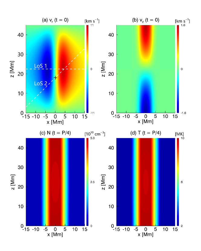
Figure 1: Snapshots of spatial distributions of the fluid parameters associated with the fast sausage mode. Shown here is a cut through the cylinder axis. The radial ($v_{r}$, panel a) and axial ($v_{z}$, panel b) velocities are for $t=0$, while the electron number density ($N$, panel c) and temperature ($T$, panel d) are for $t$ being one quarter of the wave period. All lines of sight adopted in this study are parallel to the $x-z$ plane, pertaining to slits along the $y$-direction. Two representative lines of sight, both in the $x-z$ plane, are shown by the white dashed lines. LoS 1 is perpendicular to the loop axis and passes through the loop apex, while LoS 2 makes an angle of $45^{\circ}$ with the loop and intersects the loop axis at $z_{0}=0.4L$.

The spatial distributions of the fluid parameters in the $r-z$ plane are then constructed with a spacing of $20$ km in both directions for $t$ between $0$ and $4$ periods. Advection is accounted for by employing Equations (6) and (7) during this implementation, even though a Eulerian grid is chosen for convenience (see paper I for details). Figure 1 then presents these distributions in a cut through the cylinder axis, with $x$ denoting an arbitrarily chosen perpendicular direction. The radial ($v_{r}$) and axial velocities ($v_{z}$) are shown for $t=0$, while the electron number density ($N$) and temperature ($T$) are shown for $t=P/4$. Different instants of time are necessary because of the $\pi/2$ phase difference between the relevant perturbations (see Equations 1 to 4). The continuous distribution of the equilibrium density or temperature can be readily seen, which, however, makes the expansion of the cylinder hard to tell (see Figure 1c or 1d). This happens because the maximal radial displacement is merely $\sim 32$ km.

Without loss of generality, we assume that all lines of sight are parallel to the $x-z$ plane, with two representative ones shown by the white dashed lines in Figure 1. When placed in the context of spectroscopic measurements, this means that we are placing slits along the $y$-direction. It then follows that an LoS is describable by three geometric parameters, one being the viewing angle $\theta$ between the LoS and the cylinder axis, and the other two being the combination $[y_{0},z_{0}]$ that characterizes where the LoS intersects the $y-z$ plane. For instance, LoS 1 pertains to a $\theta$ being $90^{\circ}$ and $[y_{0},z_{0}]=[0,0.5L]$. Another one (LoS 2) corresponds to a $\theta$ of $45^{\circ}$ and $[y_{0},z_{0}]=[0,0.4L]$.

2.2 Forward Modeling

The emissivity of the Fe XXI 1354 Å line is calculated at each grid point in the $r-z$ plane via

$$\epsilon=G_{\lambda 0}N^{2}~{},$$ (9)

where the contribution function $G_{\lambda 0}$ is given by

$$G_{\lambda 0}=h\nu_{ij}\cdot 0.83\cdot Ab({\rm{Fe}})f_{\mathrm{XXI}}\frac{n_{j}A_{ji}}{N}~{}.$$ (10)

Here $h\nu_{ij}$ is the energy level difference, $Ab({\rm{Fe}})$ is the abundance of Fe relative to Hydrogen, $f_{\mathrm{XXI}}$ is the ionic fraction of Fe XXI, $n_{j}$ is the fraction of Fe XXI lying in the excited state, and $A_{ji}$ is the spontaneous transition probability. We compute $G_{\lambda 0}$ using the function g_of_t from the CHIANTI package, with the ionic fraction $f_{\mathrm{XXI}}$ obtained by solving

$$\displaystyle\left(\frac{\partial}{\partial t}+{\mathbf{v}}\cdot\nabla\right)f_{q}=N\left[f_{q-1}C_{q-1}-f_{q}\left(C_{q}+R_{q}\right)+f_{q+1}R_{q+1}\right]~{},$$ (11)

where the ionization ($C$) and recombination ($R$) rate coefficients are found from CHIANTI as well (ver 8, Del Zanna et al. 2015) .

Two remarks are necessary here. First, lying behind the procedure outlined above for computing the emissivities is the coronal model approximation. In particular, the ground level of an ion is assumed to be by far the most populated, which may not be true for Fe XXI when the electron density ($N$) is sufficiently high such that populations of metastable levels are no longer negligible. This may indeed be a concern because we are examining the forbidden Fe XXI 1354 Å line. Fortunately, the outlined procedure still applies because the values adopted for $N$ are still well below the critical value of $10^{12}~{}{\rm cm}^{-3}$ (Landi et al., 2006, Table 4). Second, Equation (11) reduces to the much simpler Equilibrium-Ionization (EI) case when the wave period is much longer than the ionization and recombination timescales. We find that the Non-EI effect is marginal for Fe XXI for the examined dense flare loop, in contrast to the cases of Fe IX and Fe XII pertaining to typical active region loops as examined in paper I. In practice, we nonetheless solve Equation (11) for safety and assess the role that NEI plays afterwards. The solution procedure is initiated with the ionic fractions pertinent to the EI case as in paper I (see also Ko et al., 2010; Shen et al., 2013, for similar computations but in other contexts). It then follows that the computed ionic fractions, and hence the spectral parameters, will show no difference from the EI case if ionization equilibrium can indeed be maintained at all times.

Our forward modeling study then proceeds by converting the computed data ($\epsilon$, $T$, $v_{r}$, and $v_{z}$) from the cylindrical to the aforementioned Cartesian coordinate system, covering a grid with spacing of $20$ km in all three directions. To find the spectral profiles of the Fe XXI 1354 Å line, we then evaluate, at each grid point, the monochromatic emissivity $\epsilon_{\lambda}$ at wavelength $\lambda$ as given by (see e.g., Van Doorsselaere et al., 2016a)

$$\epsilon_{\lambda}=\frac{2\sqrt{2\ln 2}}{\sqrt{2\pi}\lambda_{w}}\epsilon\exp\left\{-\frac{4\ln 2}{\lambda_{w}^{2}}\left[\lambda-\lambda_{0}\left(1-\frac{v_{\rm LoS}}{c}\right)\right]^{2}\right\}~{}.$$ (12)

Here $\lambda_{w}=(2\sqrt{2\ln 2})\lambda_{0}(v_{\rm th}/c)$ is the thermal width, and $v_{\rm th}$ is the thermal speed determined by the instantaneous temperature. Furthermore, $\lambda_{0}$ is the rest wavelength, and $v_{\rm LoS}$ the instantaneous velocity projected onto an LoS. In what follows, by “intensity” and “monochromatic intensity” we mean

$$I=\int_{\rm LoS}\frac{\epsilon}{4\pi}dl~{},\hskip 14.22636pt\mbox{and}\hskip 14.22636ptI_{\lambda}=\int_{\rm LoS}\frac{\epsilon_{\lambda}}{4\pi}dl~{},$$ (13)

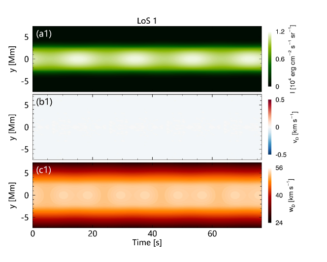
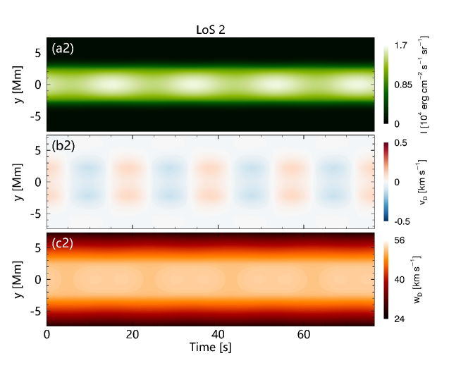
Figure 2: Temporal variations of (a) intensity $I$, (b) Doppler velocity $v_{D}$, and (c) Doppler width $w_{D}$ along the slits pertinent to LoS 1 (the upper three panels) and LoS 2 (lower).

respectively. Evidently, $\int I_{\lambda}d\lambda=I$. By “spectral profile”, we mean the dependence of $I_{\lambda}$ on $\lambda$. With IRIS in mind, we assume that when projected onto the plane-of-sky, any LoS corresponds to a square of $0.33\arcsec$ by $0.33\arcsec$ (or $240$ km $\times$ $240$ km). In addition, $I_{\lambda}$ is sampled at a spacing of $26$ mÅ for $\lambda$ between $\lambda_{0}-0.78$ Å and $\lambda_{0}$+0.78 Å. When performing the LoS integration for either $I$ or $I_{\lambda}$, we discretize an LoS into a series of thin beams, equally spaced by $20$ km and each with a size of $20$ km by $20$ km when projected onto the plane-of-sky. For each thin beam, the integration is conducted on a grid of points equally spaced by $20$ km, with the points labeled by their LoS coordinate $l$ ($l=0$ pertains to where an LoS intersects the $y-z$ plane, see the cross in Figure 1). The values thus found are then averaged over all thin beams, yield $I$ or $I_{\lambda}$. From the derived $I_{\lambda}$, we then derive the Doppler velocity $v_{\rm D}$ and width $w_{\rm D}$ by conducting a standard Gaussian fitting. When constructing the distribution of the spectral parameters along a slit, we employ a series of parallel lines-of-sight equally spaced by $240$ km. This yields $I$, $v_{\rm D}$ and $w_{\rm D}$ as functions of $y$, which labels the locations along a slit (see Figures 1 and 2).

3 Results

Now we present our forward modeling results and discuss their possible applications to the identification of FSMs using IRIS-like instruments. Figure 2 shows the temporal variations of (a) the intensity $I$, (b) Doppler velocity $v_{D}$, and (c) Doppler width $w_{D}$ along the slits pertinent to LoS 1 (the upper three panels) and LoS 2 (lower), respectively. For both slits, four blob-like intensity enhancements are seen, corresponding to the intervals of strong compression (see Figures 2a1 and 2a2). An inspection of the panels labeled (c) shows that the Doppler width variations are also similar for both slits. However, different from the intensity variations, a periodicity of half the wave period ($P/2$) can also be discerned, as indicated by the peanut-shaped features. The “peanut kernels”, namely the enhancements in Doppler width, are concentrated around the center of a given slit (i.e., $y=0$). Furthermore, any unshelled peanut sits astride an intensity enhancement. The most prominent difference in the spectral signatures between the two slits lies in the Doppler shift, which is identically zero in Figure 2b1 but not in Figure 2b2. In the former, any pertinent LoS samples the fluid parcels that flow toward and away from the observer in a symmetric manner, thereby causing no net Doppler shift. On the contrary, the contributions from the oppositely moving parcels do not exactly cancel out for the slit pertinent to LoS 2 (see Figure 1a). One also sees that the local enhancements in the magnitudes of $v_{D}$ are away from the slit center. This is understandable because the radial flow speed ($v_{r}$) is largely distributed this way and $v_{r}$ tends to dominate the velocity projected onto an LoS.

When real measurements are analyzed, it is customary to average the spectral profiles at individual pixels along a slit to enhance the signal-to-noise ratio. While the forward-modeling procedure involves little noise, we nonetheless adopt this practice by first averaging the spectral profiles in Figure 2 at a given time and then applying a Gaussian fitting afterwards. The time-series of the resulting intensity ($\bar{I}$), Doppler velocity ($\bar{v}_{D}$) and Doppler width ($\bar{w}_{D}$) are then presented in Figure 3, where we examine both (a) the slit pertinent to LoS 1 and (b) the one pertinent to LoS 2. For the ease of discussion, the instants of time $t=P/4$, $P/2$, and $3P/4$ are marked by the vertical dash-dotted lines. Note that the examined fundamental mode corresponds to the strongest rarefaction (compression) at $t=P/4$ ($t=3P/4$), but leads to no compression at $t=0$ or $P/2$. Note further that the contribution function $G_{\lambda 0}$ increases monotonically with temperature in the temperature range we examine. Examining the intensities first (the blue curves), one sees that they largely follow the density variation ($\Delta N$) but nonetheless lag behind $\Delta N$ by $\sim 18^{\circ}$. This is somewhat surprising, because one expects a phase difference of $0^{\circ}$ given the $T$-dependence of $G_{\lambda 0}$ and the fact that $\Delta N$ varies in phase with the temperature variation ($\Delta T$). It turns out that this slight phase difference results from the non-equilibrium ionization (NEI) effect, namely the ionic fraction of Fe XXI ($f_{\rm XXI}$) cannot respond instantaneously to the temperature variation. A density-dependence, albeit weak, then results for $f_{\rm XXI}$ and hence for $G_{\lambda 0}$ (see Equations 11 and 10). This happens despite that the wave period is rather long and an electron density as high as $5\times 10^{10}~{}{\rm cm}^{-3}$ is adopted. Nonetheless, the NEI effect is substantially less strong than for the response of the Fe XII 193 Å line to FSMs with much shorter periods in much less dense active region loops (see paper I). In paper I, we also showed that NEI plays no role in determining the temporal dependence of Doppler widths or Doppler shifts for both Fe IX 171 Å and Fe XII 193 Å. This is also the case for the Fe XXI 1354 Å line examined here. As shown by the red curve in Figure 3b, the Doppler velocity lags behind the density variation by exactly $90^{\circ}$, and hence behind the intensity variation by $\sim 72^{\circ}$.

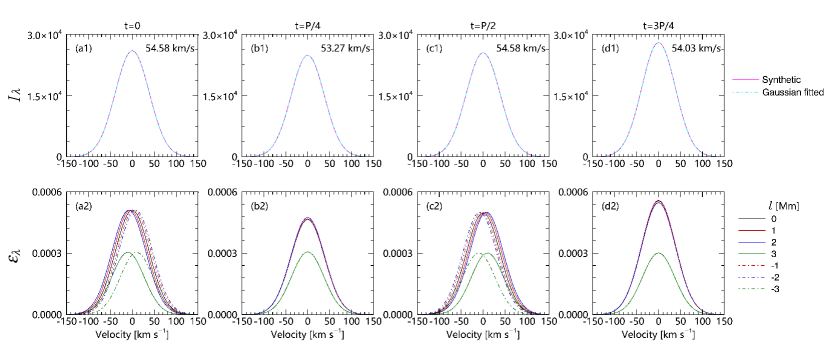
Figure 4: Wavelength dependence of the monochromatic intensities $I_{\lambda}$ (in erg$\rm~{}cm^{-2}\rm~{}s^{-1}\rm~{}\AA^{-1}\rm~{}sr^{-1}$, the upper row) and that of the monochromatic emissivities $\epsilon_{\lambda}$ (in erg$\rm~{}cm^{-3}\rm~{}s^{-1}\rm~{}\AA^{-1}$, lower) for LoS 1. Here the wavelength is presented in velocity units. In the upper row, the red curves present the synthetized profiles while the green curves are for the pertinent Gaussian-fitting. The derived Doppler widths are also printed. In the lower row, the profiles of $\epsilon_{\lambda}$ at a number of representative locations are presented as labeled. Here $l$ denotes the coordinate along the LoS, with $l=0$ corresponding to where the LoS intersects the $y-z$ plane in Figure 1. Different columns pertain to different instants of time.

The behavior of the Doppler widths, however, is somehow more complicated. While their local minima appear at both $t=P/4$ and $3P/4$, the values at $t=3P/4$ are consistently larger than at $P/4$ for both slits. This leads to the “molar”-like features between $t=2/P$ and $P$ in the green curves. Repeating once every period, these features naturally account for the periodic appearance of the “peanuts” in Figures 2c1 and 2c2. Then why does the Doppler width behave this way? This turns out to be a result of the competition between the contribution to the Doppler broadening from temperature variations and that from the bulk flow. To explain this further, we note that the temporal variation of the slit-averaged Doppler width actually follows closely the behavior of the Doppler width as sampled by the LoS that passes through the slit center. Therefore Figure 4 examines the spectral profiles at four representative instants of time (the red curves in the upper row). Here LoS 1 is taken as an example, because much is the same for LoS 2. Furthermore, the green curves pertain to the Gaussian-fitting, and the values of the derived Doppler widths are also printed. Given that the monochromatic intensity ($I_{\lambda}$) is an LoS integration of the monochromatic emissivity ($\epsilon_{\lambda}$), we also plot the wavelength-dependence of $\epsilon_{\lambda}$ at several representative locations along LoS 1 (the lower row). Evidently, the contribution to Doppler broadening from the bulk flow results from the summation of the $\epsilon_{\lambda}$ profiles shifted in opposite directions from the rest wavelength. Comparing the left two columns in Figure 4, one sees that in the first quarter of wave period, the Doppler broadening weakens and this is because both the temperature and flow speeds decrease. When time proceeds from $P/4$ towards $2/P$, both temperature and the flow speeds increase, leading the Doppler width to return to its value at $t=0$. However, when time further proceeds, the electron temperature increases but the flow speeds weaken. Consequently, the bulk flow tends to reduce the Doppler width between $t=P/2$ and $3P/4$, thereby offsetting the tendency for the Doppler width to increase with increasing temperature. What results is a local minimum in the Doppler width at $3P/4$ that exceeds the corresponding value at $P/4$.

Regarding the Doppler width ($w_{D}$), two situations are expected. If the temperature effects far exceed the effects due to the bulk flow, then one expects that $w_{D}$ will follow a simple sinusoidal shape in phase with the temperature. If, on the contrary, the bulk flow effects dominate, then $w_{D}$ is expected to possess a dominant periodicity of $P/2$ by attaining almost identical values at $t=P/4$ and $3P/4$. Our results for the Fe XXI 1354 Å line lie in between these two extremes, with the temperature effects being more important given the high temperature pertinent to flare loops. In the case of the Fe IX 171 Å and XII 193 Å lines, both Antolin & Van Doorsselaere (2013) and paper I indicated that the dominant periodicity in the Doppler widths is indeed $P/2$ when FSMs in active region loops are examined. And this periodicity of $P/2$ takes place because of the dominant role that the bulk flow plays in broadening (or narrowing) the relevant lines.

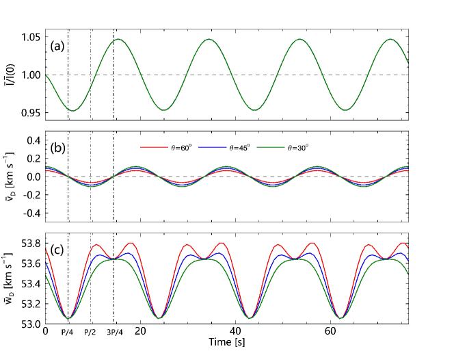
Figure 6: Similar to Figure 5 but for slits pertaining to lines of sight that make different angles ($\theta$) with the cylinder axis as labeled. All slits intersect the $x-z$ plane at $z_{0}=0.4~{}L$ with $L$ being the cylinder length.

It is also informative to study what happens for slits that pertain to different lines of sight. This is done in Figures 5 and 6 where we examine the temporal variations of (a) the intensity ($\bar{I}$), (b) Doppler velocity ($\bar{v}_{D}$) and (c) Doppler width ($\bar{w}_{D}$). The slits in Figure 5 pertain to lines of sight that are parallel to LoS 2 but intersect the cylinder axis at different locations ($z_{0}$) as indicated. On the other hand, the slits in Figure 6 are relevant for lines of sight that intersect the cylinder axis at the same location but make different angles with the cylinder. In both figures, the vertical dash-dotted lines mark the instants of time $t=P/4$, $P/2$, and $3P/4$. All the spectral parameters are derived from the slit-averaged profiles. Examine Figure 5 first. One sees that the modulations in both $\bar{I}$ and $\bar{w}_{D}$ become increasingly weak with decreasing $z_{0}$, which is understandable because the density and temperature perturbations weaken from the loop apex to footpoint. Somehow the modulation in $\bar{v}_{D}$ becomes stronger when $z_{0}$ decreases. This tendency is understandable because when $z_{0}$ decreases, the fluid parameters sampled by pertinent lines of sight become increasingly asymmetric about the $y-z$ plane. Furthermore, the phase difference between $\bar{v}_{D}$ and $\bar{I}$ are all close (although not exactly equal) to $90^{\circ}$, indicating once again the marginal role of NEI. More interesting is that, in addition to reducing the magnitude of the $\bar{w}_{D}$ variations, moving away from the loop apex also makes the dip at $3P/4$ less clear (Figure 5c). This is readily understandable with the same reasoning for explaining the molar-shaped feature for the red curve here, which is actually reproduced from Figure 3b. When time proceeds from $P/2$ to $3P/4$, while the bulk flow effects tend to narrow the line profiles, this contribution becomes increasingly weak with decreasing $z_{0}$. For $z_{0}=0.2L$, this narrowing contribution is too weak to compete with the temperature enhancements that broaden the profiles, resulting in the plateau around $t=3P/4$.

Now move on to Figure 6. One sees from Figure 6a that the intensity variations ($\bar{I}(t)/\bar{I}(t=0)$) do not depend on the viewing angle ($\theta$), despite that the absolute values of $\bar{I}(t=0)$ are different (not shown). Given that the Doppler shift $\bar{v}_{D}$ consistently lags behind the density perturbation by $90^{\circ}$, this independence on viewing angles leads to a phase difference between $\bar{I}$ and $\bar{v}_{D}$ being consistently $72^{\circ}$. (Note that the slit pertinent to $\theta=45^{\circ}$ has been examined in Figure 3b). Figure 6b further indicates that the modulations in $\bar{v}_{D}$ strengthen with decreasing $\theta$. This can also be explained with Figure 2a: with decreasing $\theta$, the fluid parameters along the pertinent lines of sight become increasingly asymmetric about the $y-z$ plane. At the expense of this slight enhancement in the Doppler shift modulations, the increasingly strong asymmetry decreases the modulations in the Doppler width as shown in Figure 6c. Now the dips at $t=3P/4$ become almost independent of $\theta$ because the flow velocities are zero at this instant of time.

From Figures 5c and 6c one sees a systematic dependence of the Doppler width variations on the viewing angle and the axial position where a pertinent LoS intersects the loop. The systematic variations of the molar-like portions are of particular interest, because they result from the systematic change in the importance of the broadening due to bulk flow relative to that resulting from temperature variations. We have shown that this should be a rather generic result for such hot emissions lines as Fe XXI 1354 Å provided that thermal effects dominate but not by far dominate the effects due to bulk flow. In reality, however, the Doppler width variations can hardly behave in the ideal way as depicted in Figures 5c and 6c. Noise and instrumental resolutions will be an issue, not to mention the difficult task of trend-removal in the time series. However, the systematic variations of the molar-like portions should also correspond to a systematic change in the importance of the periodicity of $P/2$ relative to that of the wave period $P$. Looking for the response of this additional periodicity to such factors as varying viewing angles should be more practical. For this purpose we present in Figure 7 the periodograms of the Doppler width curves presented in (a) Figure 5c and (b) Figure 6c. Note that the FFT power is normalized by its maximum for the ease of comparison between different curves. Indeed, one sees that for lines of sight with a fixed direction, the relative importance of the $P/2$ periodicity decreases when an LoS moves away from the loop apex (Figure 7a). Likewise, for lines of sight that all intersect the loop axis at $z_{0}=0.4L$, this relative importance decreases when an LoS becomes more aligned with the loop.

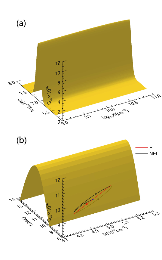
Figure 8: Contribution function ($G_{\lambda 0}$) under the assumption of equilibrium ionization (EI) for (a) the entire range of the electron density ($N$) and temperature ($T$) examined in this study, and (b) a limited range pertaining to the core of the loop. The values of $G_{\lambda 0}$ (in units of ${\rm erg}~{}{\rm cm}^{3}~{}{\rm s}^{-1}$) are returned from the function g_of_t in the Chianti package. The curves in panel b represent the trajectories in this three-dimensional space of a point initially located at the loop apex when EI (the red curve) and NEI (black) are assumed. While they both start off from the dot in the middle at $t=0$, the red track initially moves downward and forms a nearly straight line segment on the $G_{\lambda 0}$ surface, whereas the black track deviates from the $G_{\lambda 0}$ surface and eventually forms an ellipse. The difference between the two evolutionary tracks signifies the NEI effect.

All the results presented so far have been obtained with the ionic fractions by solving Equation (11). From the practical viewpoint, one may question whether addressing non-Equilibrium ionization (NEI) is necessary in the first place. Before answering this question, let us note that one important assumption behind the adopted ionization and recombination rate coefficients (see Equation 11) is that electrons are Maxwellian-distributed. However, a substantial fraction of the electrons in the flare loops examined in T16 is expected to be non-thermal as a result of the flaring processes (see e.g., Fletcher et al., 2011). While it is possible to address non-Maxwellian-distributed electrons in ionization computations (e.g., Dzifčáková & Karlický, 2018, and references therein), we nonetheless refrain from doing so for the time being. With this caveat in mind, we repeat all the emission computations by assuming EI from the outset. In what follows, we first present in Figure 8 the contribution function $G_{\lambda 0}$ (Equation 10) as a function of the electron temperature ($T$) and density ($N$) under the assumption of EI. Figure 8a examines $G_{\lambda 0}$ for the entire $[T,N]$ range pertaining to both the examined loop itself and its ambient. One sees that $G_{\lambda 0}$ shows essentially no dependence on $N$, and is sharply peaked around $\log_{10}T({\rm K})\approx 7.1$, meaning that by far the Fe XXI 1354 Å emissions come from the plasmas in the core part of the loop provided that Fe XXI is in ionization equilibrium. The same is true in our computations even though the NEI effects can be discerned. Figure 8b then presents the portion of the $G_{\lambda 0}$ distribution for the range of electron temperatures and densities restricted to the core part of the loop. In addition, we also plot the evolutionary tracks in the $[N,T,G_{\lambda 0}]$ space of a point initially located at the loop apex ($[r,z]=[0,L/2]$) for both the EI (the red curve) and NEI (black) situations. This point is representative of the fluid parcels in our computations. By construction, the red track starts off from the dot in the middle at $t=0$ and initially moves downward before eventually forming a nearly straight line segment on the $G_{\lambda 0}$ surface. The black track, on the other hand, moves away from the $G_{\lambda 0}$ surface as the loop system evolves from its initial state, and eventually forms an ellipse. The deviation of the black track from the red one signifies the NEI effect, and is seen to be rather modest.

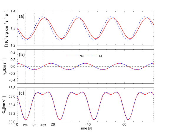
Figure 9: Similar to Figure 5 but concerning only the slit with $z_{0}=0.4L$. The red solid (blue dashed) curves pertain to the case where the ionic fractions of Fe XXI are found with the full Equation (11) (by assuming ionization equilibrium).

The NEI effect is further examined in Figure 9, where the red curves are reproduced from the spectral parameters pertaining to the case with $z_{0}=0.4L$ in Figure 5. Comparing them with the blue dashed curves representing the EI case, one sees that, as found in our paper I, NEI affects only the line intensity but not the Doppler width or Doppler shift. Furthermore, Figure 9a indicates that the most discernible difference between the NEI and EI curves lies not in the absolute value of the line intensity but in the phase difference. While the first trough in the EI result is located exactly at $t=P/4$, the NEI curve possesses a slight delay of $\sim 18^{\circ}$. Repeating the rest of the figures, we reach the same conclusion that NEI plays at most a marginal role for influencing the Fe XXI 1354 Å emissions for the adopted equilibrium parameters. In fact, a rule of thumb can be readily established by comparing the wave angular frequency ($\omega$) with the relevant ionization ($\nu_{\rm C}=NC_{21}$) and recombination ($\nu_{\rm R}=NR_{21}$) frequencies. Equation (11) indicates that the NEI effect becomes negligible when $\omega$ is much smaller than $\nu_{\rm C}$ and $\nu_{\rm R}$. Note that this requirement is more stringent than that the wave period $P=2\pi/\omega$ be much longer than the ionization and recombination timescales, $\tau_{\rm C}=1/\nu_{\rm C}$ and $\tau_{\rm R}=1/\nu_{\rm R}$. For instance, the equilibrium parameters at the loop apex lead to $\tau_{\rm C}\approx 1.6$ sec and $\tau_{\rm R}\approx 0.8$ sec, which are indeed much shorter than the period $P=19.1$ sec. The angular frequency $\omega$, on the other hand, is not that small when compared with $\nu_{\rm C}$ and $\nu_{\rm R}$, leading to the modest but discernible effect that NEI plays in determining the ionic fractions.

4 Summary and Concluding Remarks

This work was inspired by the recent IRIS detection of spectral signatures in the Fe XXI 1354 Å line of a fundamental standing fast sausage mode (FSM) trapped in flare loops (Tian et al., 2016, T16). Starting with the solutions for linear FSMs in a straight cylinder with equilibrium parameters largely compatible with T16, we have forward-modeled the modulations to the spectral parameters of this flare line. Our results suggest the following signatures in Fe XXI 1354 Å measurements for fundamental FSMs. One. The intensity variations consistently possess the same period as the FSM. Two. When the loop is sampled at non-$90^{\circ}$ angles with respect to its axis, the variations in the Doppler shift can be seen and have a nearly $90^{\circ}$ phase difference with respect to the intensity modulations. Three. In general the variations in the Doppler width possess an irregular shape due to their asymmetry in the first and second halves of a wave period ($P$). This asymmetry results in a secondary periodicity at $P/2$, whose importance relative to the dominant periodicity of $P$ shows a systematic dependence on the viewing angle and the axial location where a slit intersects the loop.

Let us remark that an additional signature is that $P$ should be as short as being comparable to the transverse fast time ($R/v_{\rm fi}$), by which we mean the time it takes perpendicularly propagating fast waves to traverse the loop in the transverse direction (e.g. Chen et al., 2016). This fourth signature was not mentioned because it has been well-established in the literature (see e.g., Meerson et al., 1978; Edwin & Roberts, 1983). Note that $v_{\rm fi}$ should be evaluated with the equilibrium parameters in the loop. Note further that this property of trapped fundamental FSMs is not to be confused with the notion that their periods are no longer than twice the longitudinal Alfvén time ($2L/v_{\rm Ae}$), which actually refers to the time it takes the Alfvén waves in the ambient corona to traverse the length of the loop. The axial phase speed of trapped FSMs equals the ambient Alfvén speed at the cutoff axial wavenumber ($k$), below which FSMs become leaky. Given that the frequency of a trapped FSM increases with increasing $k$ and that $k=\pi/L$ for the axial fundamental mode, one finds that indeed $P$ is no longer than $2L/v_{\rm Ae}$. However, theories indicate that $2L/v_{\rm Ae}$ is on the same order as $R/v_{\rm fi}$, and evaluates to $\sim 2.6R/v_{\rm fi}$ for loops with transversely discontinuous profiles (e.g., Kopylova et al., 2007). While in reality the equilibrium parameters of coronal loops are unlikely to be distributed in a discontinuous manner, taking continuous profiles into account still leads to the same conclusion (Chen et al., 2016). In fact, rather than directly using Signature 4, T16 estimated the axial phase speed and employed the derived large value as one piece of evidence that the oscillations they measured with IRIS are likely to be caused by a fundamental FSM. The considerable difference between the loop length $L$ and radius $R$, by roughly an order-of-magnitude even for the flare loops that T16 examined, means that loops need to be much denser than the ambient for FSMs to be trapped (e.g., Aschwanden et al., 2004). This was found not to be an issue for the dense flare loop examined in T16, though, as indicated by their DEM-based density estimation.

Signatures 1 and 2 are also consistent with the IRIS measurements. Indeed, T16 found a roughly periodic intensity variation, which has a phase difference of $\sim 90^{\circ}$ relative to the Doppler shift variations. We note that the phase difference we derived is $\sim 72^{\circ}$, which is slightly different from $90^{\circ}$ because Fe XXI is not in perfect ionization equilibrium despite we adopted the measured loop density ($\sim 5\times 10^{10}~{}{\rm cm}^{-3}$). The difference between the computed and measured values of the phase difference may come from the fact that the measured period ($\sim 25~{}{\rm sec}$) is slightly longer than computed here ($\sim 19.1~{}{\rm sec}$). Alternatively, it may be that the phase difference cannot be measured with precision because the cadence ($\sim 5.2~{}{\rm sec}$) is a substantial fraction of the measured period.

The cadence issue makes the comparison of Signature 3 with the IRIS measurements impossible. As shown in our Figure 7, the cadence of a spectral instrument needs to be much shorter than the wave period for the secondary periodicity to be discerned in the Doppler width variations. If boldly taking $25~{}{\rm sec}$ as being representative of standing FSMs in flare loops, a cadence of $\sim 2~{}{\rm sec}$ will be necessary. An additional issue arises if we further compare the forward modeled line parameters with T16. By choosing a small wave amplitude, we made sure that the intensities vary by only several percent to be compatible with T16. However, the measured Doppler shift variations are substantially stronger than those in the Doppler widths (Figure 3B in T16), whereas the two have roughly the same magnitude in our computations (see e.g., Figure 5). Many factors could have contributed to the cause of this discrepancy, and we name but one. As has been briefly discussed, adopting a continuous equilibrium profile is necessary to correctly compute the line parameters, the intensity in particular. This, however, introduces such free parameters as the width and profile description in the transition layer. Examining the effects of these parameters on the synthetic emissions is certainly warranted, but is nonetheless left for a future study.

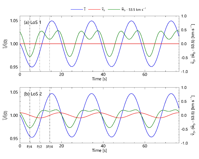
Figure 3: Temporal variations of slit-averaged intensity $\bar{I}$, Doppler velocity $\bar{v}_{D}$, and Doppler width $\bar{w}_{D}$ (offset by 53.5 km s^-1). By “slit-averaged”, we mean that these parameters are derived from the spectral profiles averaged over a slit. Two slits are examined, one pertinent to LoS 1 (panel a) and the other to LoS 2 (panel b). The three vertical dash-dotted lines mark the instants of time when $t=P/4$, $P/2$, and $3P/4$.

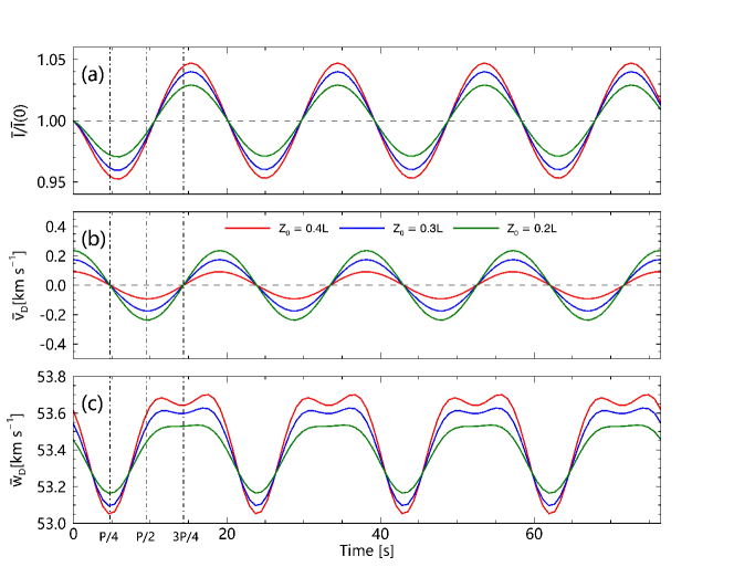
Figure 5: Temporal variations of (a) the intensity $\bar{I}$, (b) Doppler velocity $\bar{v}_{D}$, and (c) Doppler width $\bar{w}_{D}$ for slits pertaining to lines of sight that make the same angle ($45^{\circ}$) with the cylinder as LoS 2 but interest the cylinder axis at different positions ($z_{0}$). The line parameters are derived from the slit-averaged profiles. The three vertical dash-dotted lines correspond to $t=P/4$, $P/2$, and $3P/4$, respectively.

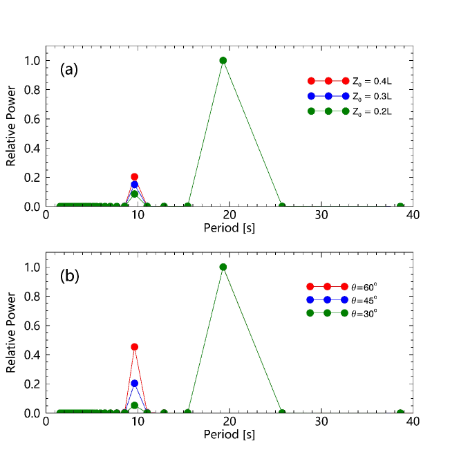
Figure 7: Fourier spectra for the Doppler width variations examined in (a) Figure 5 and (b) Figure 6. Any spectrum is normalized by its maximum, and hence the label “relative power”.

References

- Antolin & Van Doorsselaere (2013) Antolin, P., & Van Doorsselaere, T. 2013, A&A, 555, A74
- Aschwanden et al. (2004) Aschwanden, M. J., Nakariakov, V. M., & Melnikov, V. F. 2004, ApJ, 600, 458
- Banerjee et al. (2007) Banerjee, D., Erdélyi, R., Oliver, R., & O’Shea, E. 2007, Sol. Phys., 246, 3
- Bennett et al. (1999) Bennett, K., Roberts, B., & Narain, U. 1999, Sol. Phys., 185, 41
- Cally (1986) Cally, P. S. 1986, Sol. Phys., 103, 277
- Cally & Xiong (2018) Cally, P. S., & Xiong, M. 2018, Journal of Physics A Mathematical General, 51, 025501
- Chen et al. (2015) Chen, S.-X., Li, B., Xiong, M., Yu, H., & Guo, M.-Z. 2015, ApJ, 812, 22
- Chen et al. (2016) —. 2016, ApJ, 833, 114
- Cooper et al. (2003) Cooper, F. C., Nakariakov, V. M., & Tsiklauri, D. 2003, A&A, 397, 765
- De Moortel & Nakariakov (2012) De Moortel, I., & Nakariakov, V. M. 2012, Philosophical Transactions of the Royal Society of London Series A, 370, 3193
- Del Zanna et al. (2015) Del Zanna, G., Dere, K. P., Young, P. R., Landi, E., & Mason, H. E. 2015, A&A, 582, A56
- Dzifčáková & Karlický (2018) Dzifčáková, E., & Karlický, M. 2018, A&A, 618, A176
- Edwin & Roberts (1983) Edwin, P. M., & Roberts, B. 1983, Sol. Phys., 88, 179
- Erdélyi & Fedun (2007) Erdélyi, R., & Fedun, V. 2007, Sol. Phys., 246, 101
- Fletcher et al. (2011) Fletcher, L., Dennis, B. R., Hudson, H. S., et al. 2011, Space Sci. Rev., 159, 19
- Gruszecki et al. (2012) Gruszecki, M., Nakariakov, V. M., & Van Doorsselaere, T. 2012, A&A, 543, A12
- Inglis et al. (2009) Inglis, A. R., van Doorsselaere, T., Brady, C. S., & Nakariakov, V. M. 2009, A&A, 503, 569
- Kaneda et al. (2018) Kaneda, K., Misawa, H., Iwai, K., et al. 2018, ApJ, 855, L29
- Khongorova et al. (2012) Khongorova, O. V., Mikhalyaev, B. B., & Ruderman, M. S. 2012, Sol. Phys., 280, 153
- Ko et al. (2010) Ko, Y.-K., Raymond, J. C., Vršnak, B., & Vujić, E. 2010, ApJ, 722, 625
- Kolotkov et al. (2018) Kolotkov, D. Y., Nakariakov, V. M., & Kontar, E. P. 2018, ApJ, 861, 33
- Kolotkov et al. (2015) Kolotkov, D. Y., Nakariakov, V. M., Kupriyanova, E. G., Ratcliffe, H., & Shibasaki, K. 2015, A&A, 574, A53
- Kopylova et al. (2007) Kopylova, Y. G., Melnikov, A. V., Stepanov, A. V., Tsap, Y. T., & Goldvarg, T. B. 2007, Astronomy Letters, 33, 706
- Landi et al. (2006) Landi, E., Del Zanna, G., Young, P. R., et al. 2006, ApJS, 162, 261
- Li et al. (2014) Li, B., Chen, S.-X., Xia, L.-D., & Yu, H. 2014, A&A, 568, A31
- Li et al. (2013) Li, B., Habbal, S. R., & Chen, Y. 2013, ApJ, 767, 169
- McLaughlin et al. (2018) McLaughlin, J. A., Nakariakov, V. M., Dominique, M., Jelínek, P., & Takasao, S. 2018, Space Sci. Rev., 214, 45
- Meerson et al. (1978) Meerson, B. I., Sasorov, P. V., & Stepanov, A. V. 1978, Sol. Phys., 58, 165
- Melnikov et al. (2005) Melnikov, V. F., Reznikova, V. E., Shibasaki, K., & Nakariakov, V. M. 2005, A&A, 439, 727
- Nakariakov et al. (2018) Nakariakov, V. M., Anfinogentov, S., Storozhenko, A. A., et al. 2018, ApJ, 859, 154
- Nakariakov et al. (2012) Nakariakov, V. M., Hornsey, C., & Melnikov, V. F. 2012, ApJ, 761, 134
- Nakariakov & Melnikov (2009) Nakariakov, V. M., & Melnikov, V. F. 2009, Space Sci. Rev., 149, 119
- Nakariakov et al. (2003) Nakariakov, V. M., Melnikov, V. F., & Reznikova, V. E. 2003, A&A, 412, L7
- Nakariakov & Verwichte (2005) Nakariakov, V. M., & Verwichte, E. 2005, Living Reviews in Solar Physics, 2, 3
- Nakariakov et al. (2016) Nakariakov, V. M., Pilipenko, V., Heilig, B., et al. 2016, Space Sci. Rev., 200, 75
- Rosenberg (1970) Rosenberg, H. 1970, A&A, 9, 159
- Shen et al. (2013) Shen, C., Reeves, K. K., Raymond, J. C., et al. 2013, ApJ, 773, 110
- Shi et al. (2019) Shi, M., Li, B., Van Doorsselaere, T., Chen, S.-X., & Huang, Z. 2019, ApJ, 870, 99
- Su et al. (2012) Su, J. T., Shen, Y. D., Liu, Y., Liu, Y., & Mao, X. J. 2012, ApJ, 755, 113
- Terra-Homem et al. (2003) Terra-Homem, M., Erdélyi, R., & Ballai, I. 2003, Sol. Phys., 217, 199
- Terradas et al. (2005) Terradas, J., Oliver, R., & Ballester, J. L. 2005, A&A, 441, 371
- Tian et al. (2016) Tian, H., Young, P. R., Reeves, K. K., et al. 2016, ApJ, 823, L16
- Van Doorsselaere et al. (2016a) Van Doorsselaere, T., Antolin, P., Yuan, D., Reznikova, V., & Magyar, N. 2016a, Frontiers in Astronomy and Space Sciences, 3, 4
- Van Doorsselaere et al. (2016b) Van Doorsselaere, T., Kupriyanova, E. G., & Yuan, D. 2016b, Sol. Phys., 291, 3143
- Yu et al. (2015) Yu, H., Li, B., Chen, S.-X., & Guo, M.-Z. 2015, ApJ, 814, 60
- Yu et al. (2013) Yu, S., Nakariakov, V. M., Selzer, L. A., Tan, B., & Yan, Y. 2013, ApJ, 777, 159
- Yu et al. (2016) Yu, S., Nakariakov, V. M., & Yan, Y. 2016, ApJ, 826, 78
- Zajtsev & Stepanov (1975) Zajtsev, V. V., & Stepanov, A. V. 1975, Issledovaniia Geomagnetizmu Aeronomii i Fizike Solntsa, 37, 3